Importance of Loop Effects in Explaining the Accumulated Evidence for
New Physics in $B$ Decays with a Vector Leptoquark

Abstract

In recent years experiments revealed intriguing hints for new physics (NP) in $B$ decays involving $b\to c\tau\nu$ and $b\to s\ell^{+}\ell^{-}$ transitions at the $4\,\sigma$ and $5\,\sigma$ level, respectively. In addition, there are slight disagreements in $b\to u\tau\nu$ and $b\to d\mu^{+}\mu^{-}$ observables. While not significant on their own, they point in the same direction. Furthermore, $V_{us}$ extracted from $\tau$ decays shows a slight tension ($\approx 2.5\,\sigma$) with its value determined from CKM unitarity and an analysis of BELLE data found an excess in $B_{d}\to\tau^{+}\tau^{-}$. Concerning NP explanations, the vector leptoquark $SU(2)$ singlet is of special interest since it is the only single particle extension of the Standard Model which can (in principle) address all the anomalies described above. For this purpose, large couplings to $\tau$ leptons are necessary and loop effects, which we calculate herein, become important. Including them in our phenomenological analysis, we find that neither the tension in $V_{us}$ nor the excess in $B_{d}\to\tau^{+}\tau^{-}$ can be fully explained without violating bounds from $K\to\pi\nu\bar{\nu}$. However, one can account for $b\to c\tau\nu$ and $b\to u\tau\nu$ data finding intriguing correlations with $B_{q}\to\tau^{+}\tau^{-}$ and $K\to\pi\nu\bar{\nu}$. Furthermore, the explanation of $b\to c\tau\nu$ predicts a positive shift in $C_{7}$ and a negative one in $C_{9}$, being nicely in agreement with the global fit to $b\to s\ell^{+}\ell^{-}$ data. Finally, we point out that one can fully account for $b\to c\tau\nu$ and $b\to s\ell^{+}\ell^{-}$ without violating bounds from $\tau\to\phi\mu$, $\Upsilon\to\tau\mu$ or $b\to s\tau\mu$ processes.

I Introduction

So far, the LHC has not directly observed any particles beyond the Standard Model (SM). However, intriguing hints for lepton flavor universality (LFU) violating NP have been acquired:
$b\to s(d)\ell^{+}\ell^{-}$:

The ratios

$$R(K^{(*)})=\frac{{\rm Br}[B\to K^{(*)}\mu^{+}\mu^{-}]}{{\rm Br}[B\to K^{(*)}e^{+}e^{-}]}\,,$$ (1)

Aaij et al. (2014)(Aaij et al. (2017a)) indicate LFU violation with a combined significance of $\approx 4\,\sigma$ Altmannshofer et al. (2017); D’Amico et al. (2017); Ciuchini et al. (2017); Hiller and Nisandzic (2017); Geng et al. (2017); Hurth et al. (2017). Taking also into account all other $b\to s\mu^{+}\mu^{-}$ observables, like the angular observable $P_{5}^{\prime}$ Aaij et al. (2016) in the decay $B\to K^{*}\mu^{+}\mu^{-}$ , the global fit of the Wilson coefficients to all available data even shows compelling evidence Capdevila et al. (2018a) for NP ($>5\,\sigma$).

​​​​

​​​​

​​​​

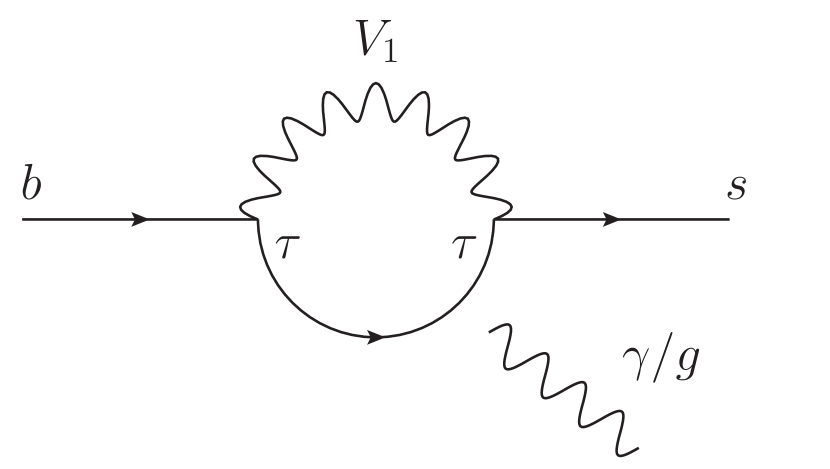
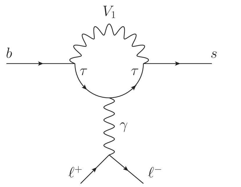
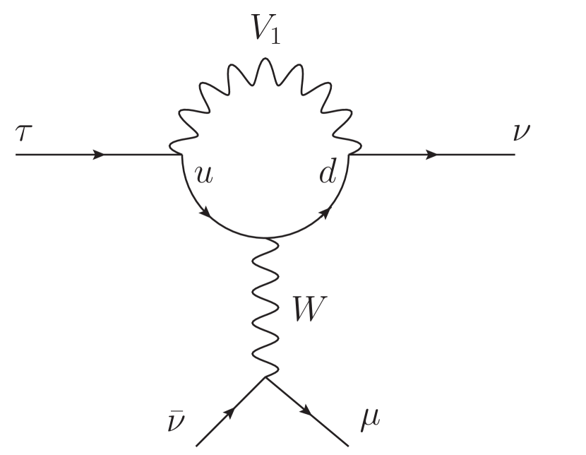
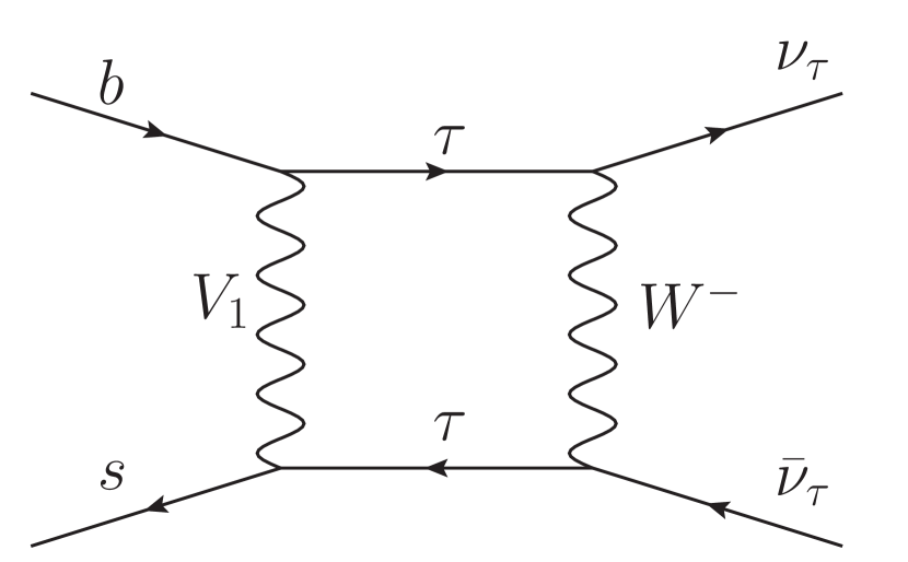
Figure 1: Feynman diagrams depicting the one-loop contributions of the vector LQ singlet to $C^{sb}_{7/8}$, $b\to s\ell^{+}\ell^{-}$, $\tau\to\mu\nu\bar{\nu}$ and $b\to s\nu\bar{\nu}$ (from left to right).

Concerning $b\to d\ell^{+}\ell^{-}$ transitions, the theoretical analysis of Ref. Hambrock et al. (2015) shows that the LHCb measurement of $B\to\pi\mu^{+}\mu^{-}$ Aaij et al. (2015) slightly differs from the theory expectation. Even though this is not significant on its own, the central value is very well in agreement with the expectation from $b\to s\ell^{+}\ell^{-}$ under the assumption of a $V_{td}/V_{ts}$-like scaling of the NP effect. In other words, an effect of the same order and sign as in $b\to s\ell^{+}\ell^{-}$, relative to the SM, is preferred. Furthermore, an (unpublished) analysis of BELLE data found an excess in $B_{d}\to\tau^{+}\tau^{-}$ Ziegler (2016).
$b\to c(u)\tau\nu$:

The ratios

$$R(D^{(*)})=\frac{{\rm Br}[B\to D^{(*)}\tau\nu]}{{\rm Br}[B\to D^{(*)}\ell\nu]}~{}~{}\text{with}~{}~{}\ell=\{e,\mu\}\,,$$ (2)

which measure LFU violation in the charged current by comparing $\tau$ modes with light leptons ($\ell=e,\mu$), differ in combination from their SM predictions by $\approx 4\,\sigma$ Amhis et al. (2017). Also, the ratio

$$R(J/\psi)=\frac{{\rm Br}[B_{c}\to J/\psi\tau\nu]}{{\rm Br}[B_{c}\to J/\psi\mu\nu]}$$ (3)

Aaij et al. (2018) exceeds the SM prediction in agreement with the expectations from $R(D^{(*)})$ Watanabe (2018); Chauhan and Kindra (2017).

Concerning $b\to u\tau\nu$ transitions, the theory prediction for $B\to\tau\nu$ crucially depends on $V_{ub}$. While previous lattice calculations resulted in rather small values of $V_{ub}$, recent calculations give a larger value (see Ref. Ricciardi (2017) for an overview). However, the measurement is still above the SM prediction by more than 1$\,\sigma$, as can be seen from the global fit Charles et al. (2005). In

$$R(\pi)=\frac{{\rm Br}[B\to\pi\tau\nu]}{{\rm Br}[B\to\pi\ell\nu]}$$ (4)

there is also a small disagreement between theory Bernlochner (2015) and experiment Hamer et al. (2016) which does not depend on $V_{ub}$. These results are not significant on their own but lie again above the SM predictions like in the case of $b\to c\tau\nu$.
$V_{us}^{\tau}$:

$V_{us}$ extracted from $\tau$ lepton decays ($V_{us}^{\tau}$) shows a tension of $2.5\,\sigma$ compared to the value of $V_{us}$ determined from CKM unitarity ($V_{us}^{\text{uni}}$) Amhis et al. (2017); Lusiani (2017).

The only possible single particle explanation, which can (at least in principle) address all these anomalies is the vector leptoquark (LQ) $SU(2)_{L}$ singlet $V_{1}$ with hypercharge $-4/3$ Alonso et al. (2015); Calibbi et al. (2015); Fajfer and Košnik (2016); Hiller et al. (2016); Bhattacharya et al. (2017); Buttazzo et al. (2017); Kumar et al. (2018) arising in the famous Pati-Salam model Pati and Salam (1974): This LQ can explain $b\to c\tau\nu$ data without violating bounds from $b\to s\nu\bar{\nu}$ and/or direct searches, provides (at tree level) a left-handed solution to $b\to s\ell^{+}\ell^{-}$ data, and does not lead to proton decay. Therefore, a sizable effect in $b\to u\tau\nu$ and $b\to d\ell^{+}\ell^{-}$ is straightforward, and also an explanation of $V_{us}^{\tau}$ could be possible. A huge enhancement of $b\to s\tau^{+}\tau^{-}$ rates is predicted as well Capdevila et al. (2018b), making an amplification of $B_{d}\to\tau^{+}\tau^{-}$ possible.

Several attempts to construct a UV completion for this LQ to address the anomalies have been made Barbieri et al. (2016, 2017); Assad et al. (2018); Di Luzio et al. (2017); Calibbi et al. (2017); Bordone et al. (2018a); Barbieri and Tesi (2018); Blanke and Crivellin (2018); Greljo and Stefanek (2018); Bordone et al. (2018b); Matsuzaki et al. (2018). In order to fully account for the $b\to c\tau\nu$ data (while respecting perturbativity), one needs sizable couplings to third generation leptons and $V_{1}$ generates, via $SU(2)_{L}$ invariance, also large contributions to the operators $d_{i}d_{j}\tau\tau$ and $u_{i}u_{j}\nu_{\tau}\nu_{\tau}$ at tree level. These operators give rise to couplings of down quarks to neutrinos or light charged leptons at loop level (see Fig. 1).

In this article we will calculate these loop effects , which turn out to be not only numerically important but also give rise to additional correlations among observables. Even though a theory with a massive vector boson without an explicit Higgs sector is not renormalizable, we still identify several phenomenologically important loop effects which are gauge independent and finite and can therefore be calculated reliably (in analogy to flavor observables within the SM).

II Model and One-Loop effects

We work in a simplified model extending the SM by a vector LQ $SU(2)_{L}$ singlet with hypercharge $-4/3$, mass $M$ and interactions with fermions determined by

$$\mathcal{L}_{V^{\mu}}=\left(\kappa_{fi}^{L}\overline{Q_{f}}\gamma_{\mu}L_{i}+\kappa_{fi}^{R}\overline{d_{f}}\gamma_{\mu}e_{i}\right)V_{1}^{\mu\dagger}+h.c.\,.$$ (5)

Here, $Q$ ($L$) are quark (lepton) $SU(2)_{L}$ doublets, $d$ ($e$) are down quark (charged lepton) singlets and $f,i$ are flavor indices. In the following, we will neglect the right-handed couplings, which are not necessary to explain the anomalies. This then generates the effective four-fermion interactions encoded in

$${\mathcal{L}_{{\rm{eff}}}}=-\frac{{{\kappa^{L}_{il}}\kappa^{L*}_{jk}}}{{{M^{2}}}}\bar{Q}_{i}^{\alpha}{\gamma^{\mu}}Q_{j}^{\beta}\bar{L}_{k}^{\beta}{\gamma_{\mu}}L_{l}^{\alpha}\,,$$ (6)

where $\alpha$ and $\beta$ label the $SU(2)$ components. After EW symmetry breaking, we work in the down basis; i.e., no CKM elements appear in flavor changing neutral currents of down quarks. We recall our definitions and the tree-level results in the appendix.

In our setup, one-loop effects involving the LQ and third generation leptons ($\tau$’s and $\tau$ neutrinos) can be very important, since we aim for large effects in $b\to c(u)\tau\nu$ and $b\to s(d)\tau^{+}\tau^{-}$ processes. In principle, a massive vector boson, like our LQ, without a Higgs sector is not renormalizable. However, in flavor physics most effects can still be calculated reliably since they are gauge independent and finite (also in unitary gauge). This is in analogy to the SM, where the contribution of the $W$ to flavor observables can be correctly calculated in unitary gauge without taking into account the Higgs sector.

We are only interested in effects which are always absent at tree level (like $b\to s\nu\bar{\nu}$ processes) or are not present at tree level due to a specific coupling structure (like $b\to s\mu^{+}\mu^{-}$ processes in the absence of muon couplings). Furthermore, we neglect tiny dimension-8 effects of the SM Higgs particle. In these cases the loop effects are the leading contributions. We calculate all diagrams at leading order in the external momenta using asymptotic expansion Smirnov (1995).

II.1 $W$ boxes contributing to $d_{i}\to d_{f}\nu\bar{\nu}$

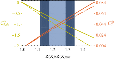
Figure 2: $C_{9,sb}^{\ell\ell}$ and $C_{7}^{sb}(\mu_{b})$ as functions of $R(X)/R(X)_{\rm SM}$ with $X=\{D,D^{*},J/\psi\}$. The solid lines correspond to $M=1\,$TeV and the dashed ones to $M=5\,$TeV while the (dark) blue region is preferred by $b\to c\tau\nu$ data at the $1\,\sigma$ ($2\,\sigma$) level. From the global fit, taking into account only lepton flavor conserving observables we have $-1.29<C_{9,sb}^{\ell\ell}<-0.87$ Descotes-Genon et al. (2016) and $-0.01<C_{7}^{sb}(\mu_{b})<0.05$ Capdevila et al. (2018a) at the $1\,\sigma$ level. Therefore, our model predicts just the right sign and size of the effect in $C_{9,sb}^{\ell\ell}$ and $C_{7}^{sb}(\mu_{b})$ necessary to explain $b\to s\ell^{+}\ell^{-}$ data, assuming an explanation of $b\to c\tau\nu$.

We use the effective Hamiltonian

$$\mathcal{H}_{{\rm eff}}^{\nu\nu} =-\dfrac{4G_{F}}{\sqrt{2}}V_{td_{k}}V_{td_{j}}^{*}\left(C^{fi}_{L,jk}\mathcal{O}_{L,jk}^{fi}+C^{fi}_{R,jk}\mathcal{O}_{R,jk}^{fi}\right)\,,$$

$$\mathcal{O}_{L,jk}^{fi} =\frac{\alpha}{4\pi}\left[\bar{d}_{j}\gamma^{\mu}P_{L}d_{k}\right]\left[\bar{\nu}_{f}\gamma_{\mu}\left(1-\gamma_{5}\right)\nu_{i}\right]\,,$$ (7)

$$\mathcal{O}_{R,jk}^{fi} =\frac{\alpha}{4\pi}\left[\bar{d}_{j}\gamma^{\mu}P_{R}d_{k}\right]\left[\bar{\nu}_{f}\gamma_{\mu}\left(1-\gamma_{5}\right)\nu_{i}\right]\,,$$

with $P_{R(L)}=(1+(-)\gamma_{5})/2$ and $G_{F}$ ($\alpha$) being the Fermi (electromagnetic fine structure) constant. The result of the box contributions involving a $W$ to $d_{i}\to d_{f}\nu\bar{\nu}$ (an example diagram is shown on the right-hand side of Fig. 1) is gauge invariant in $R_{\xi}$ gauge and the same finite result is obtained in unitary gauge (with $e=\sqrt{4\pi\alpha}$ and $m_{t}$ ($m_{W}$) the top quark ($W$ boson) mass)

$$C_{L,fa}^{ij}\!=\!\frac{{-m_{W}^{2}}}{{2{e^{2}}{V_{3a}}V_{3f}^{*}{M^{2}}}}\!\!\left(\!\!{6\kappa_{fj}^{L}\kappa_{ai}^{L*}\log\!\left(\!{\frac{{m_{W}^{2}}}{{{M^{2}}}}}\!\right)\!+\!3\left({{V_{3a}}V_{3k}^{*}\kappa_{ki}^{L*}\kappa_{fj}^{L}+V_{3f}^{*}{V_{3k}}\kappa_{kj}^{L}\kappa_{ai}^{L*}}\right)\!\frac{{\log\!\left(\!{\frac{{m_{t}^{2}}}{{m_{W}^{2}}}}\!\right)}}{{{1-\frac{m_{W}^{2}}{m_{t}^{2}}}}}\!+\!V_{3f}^{*}{V_{3k}}\kappa_{kj}^{L}{V_{3a}}V_{3l}^{*}\kappa_{li}^{L*}\frac{{m_{t}^{2}}}{{m_{W}^{2}}}}\!\!\right)$$ (8)

II.2 $W$ off-shell penguins contributing to $\tau\to\mu\nu\bar{\nu}$

Here (see third diagram in Fig. 1) we obtain again a finite and gauge independent result for the Wilson coefficient; following the analysis of Feruglio et al. (2017), we use

$${\cal H}_{{\rm{eff}}}^{\tau\mu\nu_{f}\nu_{i}}=\frac{{4{G_{F}}}}{{\sqrt{2}}}D_{L,fi}^{\tau\mu}\left[{{{\bar{\nu}}_{f}}{\gamma^{\sigma}}{P_{L}}{\nu_{i}}}\right]\left[{\bar{\mu}{\gamma_{\sigma}}{P_{L}}\tau{\mkern 1.0mu}}\right]\,,$$ (9)

with

$$D_{L,fi}^{\tau\mu}={N_{c}}{\delta_{i2}}\frac{{V_{3k}^{*}\kappa_{kf}^{L*}\kappa_{33}^{L}}}{{32{\pi^{2}}}}\frac{{m_{t}^{2}}}{{{M^{2}}}}\left(\!{1+2\log\left({\frac{{m_{t}^{2}}}{{{M^{2}}}}}\right)}\!\right){\mkern 1.0mu}.$$ (10)

We find, in agreement with Ref. Buttazzo et al. (2017), that the effect is small.

II.3 Photon and gluon penguins

We use the standard Hamiltonian (see, for example, Ref. Descotes-Genon et al. (2016)) also defined in the appendix. For on-shell photons and gluons the result of the left-hand diagram in Fig. 1 is finite in unitary gauge and the same result is obtained in $R_{\xi}$ gauge:

$$C^{sb}_{7(8)} = \frac{-\sqrt{2}}{{{G_{F}}{V_{tb}}V_{ts}^{*}{M^{2}}}}\frac{{11}}{{72}}\left(\frac{{5}}{{48}}\right){\kappa^{L}_{2i}\kappa_{3i}^{L*}}\,.$$ (11)

Taking into account the running from the LQ scale $\mu_{LQ}=M=1\,\text{TeV}$ down to $\mu_{b}=5\,\text{GeV}$ (see, e.g., Refs. Borzumati and Greub (1998); Borzumati et al. (2000)), we obtain

$$C_{7}^{sb}(\mu_{b})\approx 0.29~{}{\kappa^{L}_{2i}\kappa_{3i}^{L*}}\,.$$ (12)

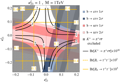
Figure 3: Predictions for $B_{q}\to\tau^{+}\tau^{-}$ and $K\to\pi\nu\bar{\nu}$ (contour lines) in the $\kappa^{L}_{13}$-$\kappa^{L}_{23}$ plane for $M=1\,{\rm TeV}$ and $\kappa^{L}_{33}=1$. The colored regions are preferred by $b\to c(u)\tau\nu$ data, where we naively averaged (i.e., we computed the weighted average of the observables and added their errors in quadrature, disregarding correlations) $R(D^{(*)})$ and $R(J/\psi)$ or $R(\pi)$ and $B\to\tau\nu$, respectively. The gray region is excluded by $K^{+}\to\pi^{+}\nu\bar{\nu}$. Here we assumed all couplings $\kappa_{ij}^{L}$ to be real.

For off-shell photons the full result (second diagram in Fig. 1) for the amplitude is gauge dependent and, in general, divergent. However, one can calculate the mixing of $C_{9,sb}^{\tau\tau}=-C_{10,sb}^{\tau\tau}$ into the four-fermion operators $O_{9,sb}^{\ell\ell}$ (containing light leptons as well) within the effective theory (i.e. after integrating out the LQ at tree level). In this way, a gauge independent result is obtained and the leading logarithm of the (unknown) full result is recovered. For off-shell photons we thus calculate the effect in the EFT (below the LQ scale), generating the following mixing into the four-fermion operators with light leptons:

$$C_{9,sb}^{\ell\ell} = \frac{\sqrt{2}}{{{G_{F}V_{tb}}V_{ts}^{*}}{M^{2}}}\frac{1}{{6}}\log\left({\frac{{{M^{2}}}}{{\mu_{b}^{2}}}}\right){\kappa_{2i}^{L}\kappa_{3i}^{L*}}\,.$$ (13)

Note that this result is model independent (at leading-log accuracy) in the sense that it does not depend on the model which generates $C_{9,sb}^{\tau\tau}=-C_{10,sb}^{\tau\tau}$. In principle, there are also $Z$ penguins generating $C_{9,sb}^{\ell\ell}$ and $C_{10,sb}^{\ell\ell}$. However, this effect is suppressed by light lepton masses (or small momenta) and is therefore of dimension 8. Further, note that there are no box diagram contributions which generate $\bar{s}b\bar{\mu}\mu$ $(\bar{s}b\bar{e}e)$ operators if the couplings of the LQ to muons (electrons) are zero at tree level.

II.4 Box diagrams with LQs

What cannot be calculated consistently are box diagrams involving only LQs Barbieri et al. (2017). Here, the results are divergent in unitary gauge which corresponds to a gauge dependence in $R_{\xi}$ gauge. However, these effects are suppressed if $|\kappa^{L}|<g_{2}$ and can be further suppressed in the presence of vectorlike fermions by a GIM-like mechanism Calibbi et al. (2017) which, in analogy to the SM, would render the result finite.

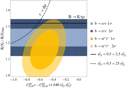
Figure 4: Allowed (colored) regions in the $C_{9,sb}^{\mu\mu}\!=\!-C_{10,sb}^{\mu\mu}$ $\left(\widehat{=}\;640\kappa_{22}^{L}\kappa_{32}^{L*}\right)$ – $R(X)/R(X)_{\rm SM}$ plane for $M=1\,$ TeV and $X=D,D^{*},J/\psi$ at the $1\,\sigma$ and $2\,\sigma$ level for $\kappa^{L}_{33}V_{cb}\ll\kappa^{L}_{23}$. The region above the black dashed (solid) line is excluded by $\tau\to\phi\mu$ ($B\to K\tau\mu$) for $\kappa^{L}_{33}=0.5=25\kappa_{32}^{L}$ ($\kappa^{L}_{33}=0.5=2.5\kappa_{32}^{L}$). The bound from $\tau\to\phi\mu$ ($B\to K\tau\mu$) depends on $\kappa_{33}^{L}$ and $\kappa_{32}^{L}$ and gets stronger if $\kappa_{32}^{L}$ gets smaller (larger). That is, for $\kappa^{L}_{33}=0.5$ and $2.7\lessapprox\kappa_{33}^{L}/\kappa_{32}^{L}\lessapprox 27$, the whole $2\,\sigma$ region preferred by $b\to c\tau\nu$ and $b\to s\ell^{+}\ell^{-}$ data is consistent with $B\to K\tau\mu$ and $\tau\to\phi\mu$.

III Phenomenology

Assuming $\kappa^{L}_{33}V_{cb}\ll\kappa^{L}_{23}$, one is safe from LHC bounds, and the effects in $B_{s}\to\tau^{+}\tau^{-}$, $C_{7}^{sb}(\mu_{b})$ (Eq. (12)) and $C_{9,sb}^{\ell\ell}$ (Eq. (13)) directly depend on $R(X)/R(X)_{\rm SM}$ (with $X=D^{(*)},J/\psi$). In Fig. 2 we show these dependences. Intriguingly, the effect generated in $C_{7}^{sb}(\mu_{b})$ and $C_{9,sb}^{\ell\ell}$, within the preferred region from $b\to c\tau\nu$ data, exactly overlaps with the $1\,\sigma$ ranges of the model independent fit to $b\to s\mu^{+}\mu^{-}$ data excluding LFU violating observables Altmannshofer and Straub (2015); Descotes-Genon et al. (2016) (therefore, only $P_{5}^{\prime}$ etc. but not $R(K^{(*)})$ can be explained).

Let us now include the effect of $\kappa_{13}^{L}$. Here, many correlations arise. First of all, $b\to c(u)\tau\nu$ is already at tree level correlated to $b\to s(d)\tau^{+}\tau^{-}$. In addition, the $W$ boxes in Eq. (8) generate effects in $B\to K^{(*)}(\pi)\nu\bar{\nu}$ and $K\to\pi\nu\bar{\nu}$. While the bounds from $B\to K^{(*)}(\pi)\nu\bar{\nu}$ turn out to be weaker than the ones from $B_{q}\to\tau^{+}\tau^{-}$, there are striking correlations with $K\to\pi\nu\bar{\nu}$, as can be seen from Fig. 3. Furthermore, we get an effect

$$\delta V_{us}^{\tau}=\frac{V_{us}^{\tau}-V_{us}^{\tau(0)}}{V_{us}^{\rm uni}}\approx-C_{us}^{\tau\tau}\,,$$ (14)

where $V_{us}^{\tau(0)}$ is the CKM matrix element extracted from $\tau$ decays without NP. However, Eq. (8) generates $K\to\pi\nu\bar{\nu}$, and respecting these bounds, the relative effect in $V_{us}^{\tau}$ can only be at the per-mill level, $\left|\delta V_{us}^{\tau}\right|\approx 0.05\%$, excluding the possibility to account for the discrepancy of $|V^{\rm uni}_{us}|=0.22547\pm 0.00095$ versus $|V^{\tau}_{us}|=0.2212\pm 0.0014$  Lusiani (2017); Amhis et al. (2017). The same is true about $B_{d}\to\tau^{+}\tau^{-}$, where the currently preferred region of analysis using BELLE data Ziegler (2016) of ${\rm{Br}}\left[{B_{d}\to\tau^{+}\tau^{-}}\right]_{\rm{exp}}=\left(4.39{}^{+0.80}_{-0.83}\pm 0.45\right)$ lies outside the plot range.

Now, in addition to the couplings $\kappa^{L}_{33}$ and $\kappa^{L}_{23}$, we allow nonvanishing $\kappa_{32}^{L}$ and $\kappa_{22}^{L}$. These couplings give rise to tree-level effects in $b\to s\mu^{+}\mu^{-}$. In Fig. 4 we show the allowed (colored) regions from $b\to s\mu^{+}\mu^{-}$ and $b\to c\tau\nu$ as well as the exclusions from $b\to s\tau\mu$ and $\tau\to\phi\mu$. Note that a simultaneous explanation of the anomalies is perfectly possible since the colored regions overlap and do not extend to the parameter space excluded by $b\to s\tau\mu$ and $\tau\to\phi\mu$. Interestingly, due to the loop effects originating from the $b\to c\tau\nu$ explanation, we predict a flavor universal effect in $C_{9,sb}^{\ell\ell}$ and $C_{7}^{sb}$ which is supplemented by a tree-level effect of the form $C_{9,sb}^{\mu\mu}=-C_{10,sb}^{\mu\mu}$ with muons only. This means that the relative NP effect compared to the SM in lepton flavor conserving observables (like $P_{5}^{\prime}$) should be larger than in $R(K^{(*)})$, which is in perfect agreement with the global fit.

IV Conclusions

The vector leptoquark $SU(2)$ singlet is a prime NP candidate to explain the current hints for LFU violation. In this article we calculated and studied the important loop effects arising within such a model and performed a phenomenological analysis. We find:

An explanation of $b\to c\tau\nu$ data generates lepton flavor universal effects in $b\to s\ell^{+}\ell^{-}$ transitions which nicely agree with the model independent fit (see Fig. 2). Therefore, the $C_{9}=-C_{10}$-like tree-level effect, which is in general LFU violating, is supplemented by these effects generating a new pattern for the Wilson coefficients. This can be tested with future data. That is, with more precise measurements of lepton flavour universality violating and lepton flavor universality conserving effects, one can test if in fact there is a lepton flavor universality conserving contribution in addition to the lepton flavor universality violating ones Algueró et al. (2018). Similar conclusions hold for the correlations between $b\to u\tau\nu$ data generating lepton flavor universal effects in $b\to d\ell^{+}\ell^{-}$ processes.

NP in $b\to c(u)\tau\nu$ generates important effects in $B_{s(d)}\to\tau^{+}\tau^{-}$ which are even correlated to $b\to s(d)\nu\bar{\nu}$ processes and $K\to\pi\nu\bar{\nu}$ via $W$ box contributions (see right-hand diagram in Fig. 1). The $V_{us}^{\tau}$ puzzle (like the CP asymmetry in $\tau\to K_{S}\pi\nu$ Cirigliano et al. (2018)) cannot be solved due to the stringent constraints from $K\to\pi\nu\bar{\nu}$, and because of $b\to u\tau\nu$ bounds one cannot fully account for the BELLE excess in $B_{d}\to\tau^{+}\tau^{-}$ (see Fig. 3).

$b\to c\tau\nu$ and $b\to s\ell^{+}\ell^{-}$ data can be simultaneously explained without violating other bounds like $\tau\to\phi\mu$ (see Fig. 4). Furthermore, one could at the same time also account for NP effects in $b\to d\mu^{+}\mu^{-}$ without violating $K_{L}\to\mu^{+}\mu^{-}$ bounds.

Acknowledgements — We are very grateful to Joaquim Matias and Bernat Capdevilla for providing us with the fit necessary for the $b\to s\ell^{+}\ell^{-}$ region in Fig. 4 whose work is supported by an explora grant (FPA2014-61478-EXP) and to Aleksey Rusov for providing us with the fit for $C_{9,bd}^{\mu\mu}$. The work of A.C. and D.M. is supported by an Ambizione Grant of the Swiss National Science Foundation (PZ00P2_154834). The work of C.G. and F.S. is supported by the Swiss National Foundation under Grant 200020_175449/1.

V Appendix

In this appendix we recall the tree-level results for the observables and give details on the experimental situation.

V.1 $d_{k}\to d_{j}\ell_{f}^{-}\ell_{i}^{+}$

We define the effective Hamiltonian as

$$\begin{split}\mathcal{H}_{{\rm eff}}^{\ell\ell}&=-\dfrac{4G_{F}}{\sqrt{2}}V_{td_{k}}V_{td_{j}}^{*}\sum^{10}\limits_{a=7}C_{a,d_{j}d_{k}}^{fi}\mathcal{O}_{a,d_{j}d_{k}}^{fi}\,,\\ {\mathcal{O}_{7(8)}^{jk}}&=\dfrac{e(g_{s})}{16\pi^{2}}m_{k}[\bar{d}_{j}{\sigma^{\mu\nu}}(T^{a})P_{R}d_{k}]F_{\mu\nu}(G^{a}_{\mu\nu})\,,\\ {\mathcal{O}_{9(10),jk}^{fi}}&=\dfrac{\alpha}{4\pi}[\bar{d}_{j}{\gamma^{\mu}}P_{L}d_{k}]\,[\bar{\ell}_{f}{\gamma_{\mu}}(\gamma_{5})\ell_{i}]\,,\end{split}$$ (15)

and obtain at tree level

$$C_{9,jk}^{fi}=-C_{10,jk}^{fi}= \dfrac{{-\sqrt{2}}}{{2{G_{F}}{V_{td_{k}}}V_{td_{j}}^{*}}}\dfrac{\pi}{\alpha}\dfrac{1}{{{M^{2}}}}\kappa_{ji}^{L}\kappa_{kf}^{L*}\,.$$ (16)

For $b\to s\mu^{+}\mu^{-}$ transitions, the allowed range is Capdevila et al. (2018a)

$$-0.37(-0.49)\geq C_{9,sb}^{\mu\mu}=-C_{10,sb}^{\mu\mu}\geq(-0.75)-0.88\,,$$ (17)

at the ($1\,\sigma$) $2\,\sigma$ level, assuming a vanishing effect in electrons. In $b\to d\mu^{+}\mu^{-}$ transitions one finds for the Wilson coefficients

$$C_{9,db}^{\mu\mu}=-C_{10,db}^{\mu\mu}=-1.9\pm 1.1\,,$$ (18)

assuming them to be real Hambrock et al. (2015). For $\tau$ leptons we have experimentally Aaij et al. (2017b)

$${\rm{Br}}{\left[{B_{s}\to{\tau^{+}}{\tau^{-}}}\right]_{{\rm{exp}}}}\leq 6.8\times{10^{-3}}\quad(95\%\,\mathrm{C.L.})\,,$$ (19)

and for $B_{d}\to\tau^{+}\tau^{-}$ there is a (unpublished) measurement of BELLE Ziegler (2016) and an upper limit of LHCb Aaij et al. (2017b)

$$\begin{split}{\rm{Br}}\left[{B_{d}\to\tau^{+}\tau^{-}}\right]^{\rm{BELLE}}_{\rm{exp}}&=\left(4.39{}^{+0.80}_{-0.83}\pm 0.45\right)\times 10^{-3}\,,\\ {\rm{Br}}\left[B_{d}\to\tau^{+}\tau^{-}\right]^{\rm{LHCb}}_{\rm{exp}}&\leq 2.1\times{10^{-3}}\quad(95\%\,\mathrm{C.L.})\,.\end{split}$$ (20)

Both are compatible at the $2\,\sigma$ level. The SM predictions are given by Bobeth et al. (2014); Bobeth (2014) In our model, we have

$$\dfrac{{\rm{Br}}\left[{{B_{q}}\to{\tau^{+}}{\tau^{-}}}\right]}{{\rm{Br}}{\left[{{B_{q}}\to{\tau^{+}}{\tau^{-}}}\right]_{\rm SM}}}=\left|{{1+\frac{{C_{10,qb}^{\tau\tau}}}{{C_{10,qb}^{\rm SM}}}}}\right|^{2}\,,$$ (22)

with $q=s,d$ and $C_{10,qb}^{\rm SM}\approx-4.3$ Bobeth et al. (2000); Huber et al. (2006). For the analysis of $B\to K^{(*)}\tau\mu$ we will use the results of Ref. Crivellin et al. (2015).

The short distance contribution to the branching ratio of $K_{L}\to\mu^{+}\mu^{-}$ is given by Buras et al. (2015a) (with the Hamiltonian defined e.g. in Ref. Blanke et al. (2009))

$${\rm{Br}}\left[K_{L}\to\mu^{+}\mu^{-}\right]_{\rm{SD}}=a_{L}\left(\frac{{\mathop{\rm Re}\nolimits}\left[\lambda_{t}\tilde{Y}\right]}{\lambda^{5}}+\frac{{\mathop{\rm Re}\nolimits}\left[\lambda_{c}\right]}{\lambda}P_{c}^{Y}\right)^{2}$$

with the numerical input

$$a_{L} = 2.01\times 10^{-9}\,,\;\tilde{Y}=Y_{SM}-s_{W}^{2}C_{10,sd}^{\mu\mu}\,,$$

$$Y_{SM} = 1.018\left(\frac{m_{t}}{170\,{\rm{GeV}}}\right)^{1.56}\,,\;P_{c}^{Y}=0.115\pm 0.017\,,$$

$$\lambda_{i} = V_{is}^{*}V_{id}\,,\;\lambda=\left|V_{us}\right|\,.$$ (23)

The upper experimental limit for the short distance contribution is Isidori and Unterdorfer (2004)

$${\rm{Br}}\left[K_{L}\to\mu^{+}\mu^{-}\right]_{\rm{SD}}<2.5\times 10^{-9}\,.$$ (24)

Using Ref.Bhattacharya et al. (2017) we have

$${\rm{Br}}\left[\tau\!\to\!\phi\mu\right]=\frac{f_{\phi}^{2}m_{\tau}^{3}\tau_{\tau}}{128\pi}\frac{\left|\kappa_{22}^{L}\kappa_{23}^{L*}\right|^{2}}{M^{4}}\left(\!\!1-\frac{m_{\phi}^{2}}{m_{\tau}^{2}}\right)^{\!2}\!\!\left(\!\!1+2\frac{m_{\phi}^{2}}{m_{\tau}^{2}}\!\right)$$

with the current experimental limit Miyazaki et al. (2011)

$${\rm{Br}}\left[\tau\to\phi\mu\right]<8.4\times 10^{-8}\quad(90\%\,\mathrm{C.L.})\,.$$ (25)

If we consider $\Upsilon(nS)\to\tau\mu$, we have Kumar et al. (2018)

$${\rm{Br}}\left[\Upsilon(3S)\to\tau\mu\right] = 2.6\times 10^{-7}\frac{\big{|}\kappa^{L}_{32}\kappa^{L*}_{33}\big{|}^{2}}{M^{4}(\,\text{TeV})}\,.$$ (26)

Comparing this to the experimental limit ${\rm{Br}}\left[\Upsilon(3S)\to\tau\mu\right]<3.1\times 10^{-6}~{}(90\%\,\mathrm{C.L.})$ of Ref. Lees et al. (2010), this does not pose relevant constraints on our model.

V.2 $d_{k}\to d_{j}\nu_{i}\bar{\nu}_{f}$

We use the conventions

$$\begin{split}\mathcal{H}_{{\rm eff}}^{\nu\nu}&=-\dfrac{4G_{F}}{\sqrt{2}}V_{td_{k}}V_{td_{j}}^{*}\left(C^{fi}_{L,jk}\mathcal{O}_{L,jk}^{fi}+C^{fi}_{R,jk}\mathcal{O}_{R,jk}^{fi}\right)\,,\\ \mathcal{O}_{L(R),jk}^{fi}&=\frac{\alpha}{4\pi}\left[\bar{d}_{j}\gamma^{\mu}P_{L(R)}d_{k}\right]\left[\bar{\nu}_{f}\gamma_{\mu}\left(1-\gamma_{5}\right)\nu_{i}\right]\,.\end{split}$$ (27)

Note that the LQ does not contribute at tree level.

For $K\to\pi\nu\bar{\nu}$ we use Ref. Buras et al. (2005) with the updated numerical values given in Ref. Buras et al. (2015b) resulting in

$$\!\!\!\!\!\!\!\!{\rm{Br}}\left[{{K^{\pm}}\to{\pi^{\pm}}\nu\bar{\nu}}\right]=\frac{1}{3}\left({1+{\Delta_{EM}}}\right){\eta_{\pm}}\times$$

$$\!\!\!\!\!\sum\limits_{f,i=1}^{3}\left[\left(\frac{{\mathop{\rm Im}\nolimits}{{\left[{{\lambda_{t}}\tilde{X}_{L}^{fi}}\right]}}}{\lambda^{5}}\right)^{\!\!2}\!\!\!+\!\left(\frac{{\mathop{\rm Re}\nolimits}\left[{{\lambda_{c}}}\right]}{\lambda}{P_{c}}{\delta_{fi}}+\frac{{\mathop{\rm Re}\nolimits}\left[{{\lambda_{t}}\tilde{X}_{L}^{fi}}\right]}{\lambda^{5}}\right)^{\!\!\!2}\right],$$

$${\rm{Br}}\left[{{K_{L}}\to\pi\nu\bar{\nu}}\right]=\frac{1}{3}{\eta_{L}}\sum\limits_{f,i=1}^{3}\left({\frac{{\mathop{\rm Im}\nolimits}{{\left[{{\lambda_{t}}\tilde{X}_{L}^{fi}}\right]}}}{\lambda^{5}}}\right)^{\!\!2}\,,$$ (28)

with

$$\begin{aligned} \tilde{X}_{L}^{fi}&=X_{L}^{{\rm{SM}},fi}-{s_{W}^{2}}{C_{L,sd}^{fi}}\,,\;{P_{c}}=0.404\pm 0.024\\ {\eta_{\pm}}&=\left({5.173\pm 0.025}\right){10^{-11}}{\left[{\frac{\lambda}{{0.225}}}\right]^{8}}\,,\\ {\eta_{L}}&=\left({2.231\pm 0.013}\right){10^{-10}}{\left[{\frac{\lambda}{{0.225}}}\right]^{8}\,,}\\ {\Delta_{EM}}&=-0.003\,,\;X_{L}^{{\rm{SM}},fi}=\left({1.481\pm 0.005\pm 0.008}\right){\delta_{fi}}\,.\end{aligned}$$ (29)

For $B\to K^{(*)}\nu\bar{\nu}$ we follow Ref. Buras et al. (2015c), giving $C_{L,sb}^{{\rm SM},fi}\approx-1.47/s_{W}^{2}\delta_{fi}$, and the branching ratios normalized by the SM predictions read

$${R_{K^{(*)}}^{\nu\bar{\nu}}}=\frac{1}{3}\sum\limits_{f,i=1}^{3}\dfrac{\big{|}{C_{L,sb}^{fi}}\big{|}^{2}}{\big{|}{C_{L,sb}^{{\rm SM},fi}}\big{|}^{2}}\,.$$ (30)

This has to be compared to the current experimental limits ${R_{K}^{\nu\bar{\nu}}}<3.9$ and ${R_{{K^{*}}}^{\nu\bar{\nu}}}<2.7$ Grygier et al. (2017) (both at $90\%\,\mathrm{C.L.}$). The future BELLE II sensitivity for $B\to K^{(*)}\nu\bar{\nu}$ is 30% of the SM branching ratio Abe et al. (2010).

V.3 $d_{k}\to u_{j}\bar{\nu}\ell^{-}$

We define the effective Hamiltonian as

$${\mathcal{H}_{{\rm{eff}}}^{\ell_{f}\nu_{i}}}=\dfrac{{4{G_{F}}}}{{\sqrt{2}}}{V_{jk}}C_{jk}^{fi}\left[{\bar{u}_{j}{\gamma^{\mu}}{P_{L}}d_{k}}\right]\left[{{{\bar{\ell}}_{f}}{\gamma_{\mu}}{P_{L}}{\nu_{i}}}\right]\,,$$ (31)

where in the SM $C_{jk,{\rm SM}}^{fi}=\delta_{fi}$. The contribution of our model is given by

$$C_{jk}^{fi}=\frac{\sqrt{2}}{4G_{F}M^{2}}\frac{V_{jl}}{V_{jk}}\kappa^{L}_{li}\kappa^{L*}_{kf}\,.$$ (32)

With these conventions we have for $b\to c\tau\nu$ transitions

$${R\left({{X}}\right)\mathord{\left/{\vphantom{{R\left({{X}}\right)}{R{{\left({{D^{\left(*\right)}}}\right)}_{{\rm{SM}}}}}}}\right.\kern-1.2pt}{R{{\left({{X}}\right)}_{{\rm{SM}}}}}}=\sum\limits_{i=1}^{3}{{{\left|{{\delta_{3i}}+C_{cb}^{\tau i}}\right|}^{2}}}\,,$$ (33)

with $X=\{D,D^{*},J/\psi\}$, assuming vanishing contributions to the muon and electron channels. We obtain the analogous expression for $b\to u\tau\nu$.

Concerning $\tau\to K(\pi)\nu$ we find that the CKM element $V_{us}^{\tau}$ extracted from these decays is given in terms of the one determined in the absence of NP contributions ($V_{us}^{\tau(0)}$) by

$$V_{us}^{\tau}=V_{us}^{\tau(0)}/(1+C_{us}^{\tau\tau})\,,$$ (34)

where we neglected LFV effects. This has to be compared to Lusiani (2017); Amhis et al. (2017) $|V^{\rm uni}_{us}|=0.22547\pm 0.00095$ and $|V^{\tau}_{us}|=0.2212\pm 0.0014$.

In Ref. Bernlochner (2015) the analysis gives

$$\begin{split}R\left(\pi\right)_{\rm{exp}}&=1.05\pm 0.51\,,\\ R\left(\pi\right)_{\rm{SM}}&=0.641\pm 0.016\,.\end{split}$$ (35)

For $B\to\tau\nu$ we use the PDG value Patrignani et al. (2016) and the SM prediction of Ref. Charles et al. (2005) at the $2\,\sigma$ level

$$\begin{split}{\rm{Br}[B\to\tau\nu]_{\rm exp}}&=\left(1.09\pm 0.24\right)\times 10^{-4}\,,\\ {\rm{Br}[B\to\tau\nu]_{\rm SM}}&=\left(0.851^{+0.079}_{-0.077}\right)\times 10^{-4}\,.\end{split}$$ (36)

References

- Aaij et al. (2014) R. Aaij et al. (LHCb), Phys. Rev. Lett. 113, 151601 (2014), eprint 1406.6482.
- Aaij et al. (2017a) R. Aaij et al. (LHCb), JHEP 08, 055 (2017a), eprint 1705.05802.
- Altmannshofer et al. (2017) W. Altmannshofer, P. Stangl, and D. M. Straub, Phys. Rev. D96, 055008 (2017), eprint 1704.05435.
- D’Amico et al. (2017) G. D’Amico, M. Nardecchia, P. Panci, F. Sannino, A. Strumia, R. Torre, and A. Urbano, JHEP 09, 010 (2017), eprint 1704.05438.
- Ciuchini et al. (2017) M. Ciuchini, A. M. Coutinho, M. Fedele, E. Franco, A. Paul, L. Silvestrini, and M. Valli, Eur. Phys. J. C77, 688 (2017), eprint 1704.05447.
- Hiller and Nisandzic (2017) G. Hiller and I. Nisandzic, Phys. Rev. D96, 035003 (2017), eprint 1704.05444.
- Geng et al. (2017) L.-S. Geng, B. Grinstein, S. Jäger, J. Martin Camalich, X.-L. Ren, and R.-X. Shi, Phys. Rev. D96, 093006 (2017), eprint 1704.05446.
- Hurth et al. (2017) T. Hurth, F. Mahmoudi, D. Martinez Santos, and S. Neshatpour, Phys. Rev. D96, 095034 (2017), eprint 1705.06274.
- Aaij et al. (2016) R. Aaij et al. (LHCb), JHEP 02, 104 (2016), eprint 1512.04442.
- Capdevila et al. (2018a) B. Capdevila, A. Crivellin, S. Descotes-Genon, J. Matias, and J. Virto, JHEP 01, 093 (2018a), eprint 1704.05340.
- Hambrock et al. (2015) C. Hambrock, A. Khodjamirian, and A. Rusov, Phys. Rev. D92, 074020 (2015), eprint 1506.07760.
- Aaij et al. (2015) R. Aaij et al. (LHCb), JHEP 10, 034 (2015), eprint 1509.00414.
- Ziegler (2016) M. Ziegler, Ph.D. thesis, KIT, Karlsruhe (2016), URL http://belle.kek.jp/belle/theses/doctor/ziegler16.pdf.
- Amhis et al. (2017) Y. Amhis et al. (HFLAV), Eur. Phys. J. C77, 895 (2017), eprint 1612.07233.
- Aaij et al. (2018) R. Aaij et al. (LHCb), Phys. Rev. Lett. 120, 121801 (2018), eprint 1711.05623.
- Watanabe (2018) R. Watanabe, Phys. Lett. B776, 5 (2018), eprint 1709.08644.
- Chauhan and Kindra (2017) B. Chauhan and B. Kindra (2017), eprint 1709.09989.
- Ricciardi (2017) G. Ricciardi, Mod. Phys. Lett. A32, 1730005 (2017), eprint 1610.04387.
- Charles et al. (2005) J. Charles, A. Hocker, H. Lacker, S. Laplace, F. R. Le Diberder, J. Malcles, J. Ocariz, M. Pivk, and L. Roos (CKMfitter Group), Eur. Phys. J. C41, 1 (2005), eprint hep-ph/0406184.
- Bernlochner (2015) F. U. Bernlochner, Phys. Rev. D92, 115019 (2015), eprint 1509.06938.
- Hamer et al. (2016) P. Hamer et al. (Belle), Phys. Rev. D93, 032007 (2016), eprint 1509.06521.
- Lusiani (2017) A. Lusiani, Nucl. Part. Phys. Proc. 287-288, 29 (2017).
- Alonso et al. (2015) R. Alonso, B. Grinstein, and J. Martin Camalich, JHEP 10, 184 (2015), eprint 1505.05164.
- Calibbi et al. (2015) L. Calibbi, A. Crivellin, and T. Ota, Phys. Rev. Lett. 115, 181801 (2015), eprint 1506.02661.
- Fajfer and Košnik (2016) S. Fajfer and N. Košnik, Phys. Lett. B755, 270 (2016), eprint 1511.06024.
- Hiller et al. (2016) G. Hiller, D. Loose, and K. Schönwald, JHEP 12, 027 (2016), eprint 1609.08895.
- Bhattacharya et al. (2017) B. Bhattacharya, A. Datta, J.-P. Guévin, D. London, and R. Watanabe, JHEP 01, 015 (2017), eprint 1609.09078.
- Buttazzo et al. (2017) D. Buttazzo, A. Greljo, G. Isidori, and D. Marzocca, JHEP 11, 044 (2017), eprint 1706.07808.
- Kumar et al. (2018) J. Kumar, D. London, and R. Watanabe (2018), eprint 1806.07403.
- Pati and Salam (1974) J. C. Pati and A. Salam, Phys. Rev. D10, 275 (1974), [Erratum: Phys. Rev.D11,703(1975)].
- Capdevila et al. (2018b) B. Capdevila, A. Crivellin, S. Descotes-Genon, L. Hofer, and J. Matias, Phys. Rev. Lett. 120, 181802 (2018b), eprint 1712.01919.
- Barbieri et al. (2016) R. Barbieri, G. Isidori, A. Pattori, and F. Senia, Eur. Phys. J. C76, 67 (2016), eprint 1512.01560.
- Barbieri et al. (2017) R. Barbieri, C. W. Murphy, and F. Senia, Eur. Phys. J. C77, 8 (2017), eprint 1611.04930.
- Assad et al. (2018) N. Assad, B. Fornal, and B. Grinstein, Phys. Lett. B777, 324 (2018), eprint 1708.06350.
- Di Luzio et al. (2017) L. Di Luzio, A. Greljo, and M. Nardecchia, Phys. Rev. D96, 115011 (2017), eprint 1708.08450.
- Calibbi et al. (2017) L. Calibbi, A. Crivellin, and T. Li (2017), eprint 1709.00692.
- Bordone et al. (2018a) M. Bordone, C. Cornella, J. Fuentes-Martin, and G. Isidori, Phys. Lett. B779, 317 (2018a), eprint 1712.01368.
- Barbieri and Tesi (2018) R. Barbieri and A. Tesi, Eur. Phys. J. C78, 193 (2018), eprint 1712.06844.
- Blanke and Crivellin (2018) M. Blanke and A. Crivellin (2018), eprint 1801.07256.
- Greljo and Stefanek (2018) A. Greljo and B. A. Stefanek, Phys. Lett. B782, 131 (2018), eprint 1802.04274.
- Bordone et al. (2018b) M. Bordone, C. Cornella, J. Fuentes-Martín, and G. Isidori (2018b), eprint 1805.09328.
- Matsuzaki et al. (2018) S. Matsuzaki, K. Nishiwaki, and K. Yamamoto (2018), eprint 1806.02312.
- Smirnov (1995) V. A. Smirnov, Mod. Phys. Lett. A10, 1485 (1995), eprint hep-th/9412063.
- Descotes-Genon et al. (2016) S. Descotes-Genon, L. Hofer, J. Matias, and J. Virto, JHEP 06, 092 (2016), eprint 1510.04239.
- Feruglio et al. (2017) F. Feruglio, P. Paradisi, and A. Pattori, JHEP 09, 061 (2017), eprint 1705.00929.
- Borzumati and Greub (1998) F. Borzumati and C. Greub, Phys. Rev. D58, 074004 (1998), eprint hep-ph/9802391.
- Borzumati et al. (2000) F. Borzumati, C. Greub, T. Hurth, and D. Wyler, Phys. Rev. D62, 075005 (2000), eprint hep-ph/9911245.
- Altmannshofer and Straub (2015) W. Altmannshofer and D. M. Straub, Eur. Phys. J. C75, 382 (2015), eprint 1411.3161.
- Algueró et al. (2018) M. Algueró, B. Capdevila, S. Descotes-Genon, P. Masjuan, and J. Matias (2018), eprint 1809.08447.
- Cirigliano et al. (2018) V. Cirigliano, A. Crivellin, and M. Hoferichter, Phys. Rev. Lett. 120, 141803 (2018), eprint 1712.06595.
- Aaij et al. (2017b) R. Aaij et al. (LHCb), Phys. Rev. Lett. 118, 251802 (2017b), eprint 1703.02508.
- Bobeth et al. (2014) C. Bobeth, M. Gorbahn, T. Hermann, M. Misiak, E. Stamou, and M. Steinhauser, Phys. Rev. Lett. 112, 101801 (2014), eprint 1311.0903.
- Bobeth (2014) C. Bobeth, in Proceedings, 49th Rencontres de Moriond on Electroweak Interactions and Unified Theories: La Thuile, Italy, March 15-22, 2014 (2014), pp. 75–80, eprint 1405.4907, URL https://inspirehep.net/record/1297237/files/arXiv:1405.4907.pdf.
- Bobeth et al. (2000) C. Bobeth, M. Misiak, and J. Urban, Nucl. Phys. B574, 291 (2000), eprint hep-ph/9910220.
- Huber et al. (2006) T. Huber, E. Lunghi, M. Misiak, and D. Wyler, Nucl. Phys. B740, 105 (2006), eprint hep-ph/0512066.
- Crivellin et al. (2015) A. Crivellin, L. Hofer, J. Matias, U. Nierste, S. Pokorski, and J. Rosiek, Phys. Rev. D92, 054013 (2015), eprint 1504.07928.
- Buras et al. (2015a) A. J. Buras, D. Buttazzo, and R. Knegjens, JHEP 11, 166 (2015a), eprint 1507.08672.
- Blanke et al. (2009) M. Blanke, A. J. Buras, B. Duling, K. Gemmler, and S. Gori, JHEP 03, 108 (2009), eprint 0812.3803.
- Isidori and Unterdorfer (2004) G. Isidori and R. Unterdorfer, JHEP 01, 009 (2004), eprint hep-ph/0311084.
- Miyazaki et al. (2011) Y. Miyazaki et al. (Belle), Phys. Lett. B699, 251 (2011), eprint 1101.0755.
- Lees et al. (2010) J. P. Lees et al. (BaBar), Phys. Rev. Lett. 104, 151802 (2010), eprint 1001.1883.
- Buras et al. (2005) A. J. Buras, T. Ewerth, S. Jager, and J. Rosiek, Nucl. Phys. B714, 103 (2005), eprint hep-ph/0408142.
- Buras et al. (2015b) A. J. Buras, D. Buttazzo, J. Girrbach-Noe, and R. Knegjens, JHEP 11, 033 (2015b), eprint 1503.02693.
- Buras et al. (2015c) A. J. Buras, J. Girrbach-Noe, C. Niehoff, and D. M. Straub, JHEP 02, 184 (2015c), eprint 1409.4557.
- Grygier et al. (2017) J. Grygier et al. (Belle), Phys. Rev. D96, 091101 (2017), [Addendum: Phys. Rev.D97,no.9,099902(2018)], eprint 1702.03224.
- Abe et al. (2010) T. Abe et al. (Belle-II) (2010), eprint 1011.0352.
- Patrignani et al. (2016) C. Patrignani et al. (Particle Data Group), Chin. Phys. C40, 100001 (2016).
- Bobeth and Buras (2018) C. Bobeth and A. J. Buras, JHEP 02, 101 (2018), eprint 1712.01295.
- Fajfer et al. (2018) S. Fajfer, N. Košnik, and L. Vale Silva, Eur. Phys. J. C78, 275 (2018), eprint 1802.00786.
- Earl and Gregoire (2018) K. Earl and T. Gregoire (2018), eprint 1806.01343.