RKKY interaction in Mn-doped 4 $\times$ 4 Luttinger systems

Abstract

We consider Mn-doped bulk zinc-blende semiconductors described by the 4 $\times$ 4 Luttinger Hamiltonian. In these semiconductors, Mn atom acts as an acceptor providing the system a mobile hole, and also acts like a magnetic impurity of spin $S=5/2$. We obtain exact analytical expressions of the hole mediated Ruderman-Kittel-Kasuya-Yoshida (RKKY) exchange interaction between two Mn²⁺ ions. The RKKY interaction of the Luttinger system consists of collinear Heisenberg-like and Ising-like interactions. The characteristic beating patterns appear in the range functions of the RKKY interaction owing to the presence of multiple Fermi wave-vectors of the underlying $j=3/2$ states. As an application of the analytical form of the range function, from the finite temperature evaluation of the correlation functions, we calculate the contribution of RKKY interaction to the Curie-Weiss temperatures of a particular dilute magnetic semiconductor ZnMnTe where $4\times 4$ Luttinger Hamiltonian is valid.

I Introduction

An electric control of the spin degree of freedom of a charge carrier is one of the primary objectives in spintronics and quantum information processing. The inherent spin-orbit interaction (SOI) arises due to the relativistic effect, which can be controlled by the spatial inversion symmetry breaking external electric field. The SOIs in materials give rise to many exotic phenomena. For example, the intrinsic spin Hall effect (SHE) arises solely due to the spin-orbit coupling even in absence of any magnetic impurities. After the theoretical proposal of intrinsic SHE murakami1 in $p$-doped III-V semiconductors described by the Luttinger Hamiltonian Lutin for the spin-3/2 valence band, there is a resurgent research interest on various properties of the Luttinger Hamiltonian Lutin . This exotic phenomena has been realized experimentally in bulk n-doped semiconductors such as GaAs and InGaAs she-exp as well as in two-dimensional hole gas she-exp1 . The hole gas is preferred over electron gas in the study of spin-related phenomena. This is because the $p$-orbital states of the hole wave function reduces the contact hyperfine interaction spin-coh ; spin-coh1 . This in turn enhances the spin coherence time of the hole charge carrier spin-coh-exp ; spin-coh-exp1 . A large number of theoretical studies e.g. spin Hall conductivity murakami2 , wave packet dynamics zb1 ; zb2 ; zb3 , Hartree-Fock analysis jSc1 , beating pattern in Friedel oscillations jSc2 ; jSc3 , magnetotransport coefficients sdh , electrical and optical conductivities opt of the Luttinger Hamiltonian have been carried out in recent past studies.

The mechanism of interaction between two localized magnetic impurities in spintronics materials attract considerable attention. The RKKY interaction Ruderman ; kasuya ; yosida is an indirect exchange interaction between two magnetic impurities mediated by mobile charge carriers. This long-range spin-spin interaction plays a crucial role in magnetic ordering (ferromagnetic/antiferromagnetic) of the impurities and may help to understand the magnetic properties of the host system. The nature of the mobile carriers (e.g. helicity, energy dispersion, spinor structure etc) determine the characteristics of the RKKY interaction. The role of the RKKY interaction in other condensed matter systems has also been studied extensively. For instance, magnetoresistance in multilayer structures multilayer , topological states and Majorana fermions Majorana . The Rashba spin-orbit coupling effect on RKKY interaction has been rigorously studied in 1D rkky1 ; rkky1-egger ; rkky1-lin ; rkky1-loss , 2D rkky2 ; rkky2-loss ; rkky2-kern ; multi-graphene ; sonu2018 ; Firoz-phosp and 3D rkky3 electron systems. The strength of the range functions characterizing RKKY interaction in various systems oscillate with the distance between two magnetic impurities $(R)$ and decays asymptotically as $1/R^{\eta}$ with $\eta$ being the system dependent exponent. The oscillation frequency (in units of the distance $R$) is determined by the density and effective mass of the charge carriers and other material parameters.

The ferromagnetic ordering in Mn-doped zinc-blende semiconductors was first realized by Muneketa et al 1st-exp . Subsequently it has been established that Mn atom is the source of local magnetic moments and also provides mobile holes in many Mn-doped zinc-blende semiconductors (such as GaAs, GaP and ZnTe) and show up the Curie-Weiss temperatures from few kelvins to few hundred kelvins 110 ; fms-e ; fms-e1 ; fms-e2 ; fms-e3 ; fms-e4 ; exp-theory ; fms-rev ; fms-e5 ; GaP1 ; GaP2 .

There have been extensive theoretical studies of ferromagnetism in Mn-doped zinc blende semiconductors fms-rev , which estimate the Curie-Weiss transition temperature closed to the experimental findings. The Ginzburg-Landau theory GL has been used to describe ferromagnetic properties of Mn-doped semiconductors. A simple model in the low-Mn density regime was proposed hop , in which holes are allowed to hop to the magnetic impurity sites and interact with the magnetic moments via phenomenological exchange interactions. There are other models based on a polaronic picture where a cloud of Mn-spins are polarized by a single hole polaronic . The concept of magnetic percolation picture was introduced to estimate the observed Curie-Weiss temperature percolation . The ferromagnetic semiconductors have also been studied theoretically using the ${\bf k}\cdot{\bf p}$ kinetic-exchange effective Hamiltonian dietl-6x6 ; dietl0 . There have been several studies to explain the ferromagnetism in zinc-blende semiconductors using the RKKY exchange interaction diet ; exp-theory ; avinash ; timm .

An analytical study of RKKY interaction mediated by the states of underlying Luttinger Hamiltonian is still lacking. In this work, we provide an exact analytical expression of the RKKY exchange interaction between two magnetic Mn²⁺ ions in 3D hole-gas (3DHG) that follows the $4\times 4$ Luttinger Hamiltonian. It’s form is different from that of 3DEG owing to the multiband nature of the Luttinger system. Our result displays the explicit dependence on the relevant band structure parameters of the Luttinger Hamiltonian. Using the analytical expression of the range function, we determine the contribution of RKKY interaction to the Curie-Weiss temperatures $T_{C}$ for a ferromagnetic semiconductor ZnMnTe.

The remainder of this paper is organized as follows. In section II, we briefly describe the Kohn-Luttinger Hamiltonian and its basic ground state properties. In section III, we derive an analytical expression of the RKKY interaction in Mn-doped zinc blende semiconductors described by $4\times 4$ Kohn-Luttinger Hamiltonian. In section IV, we compute $T_{C}$ for ZnMnTe and summarize our results in section V.

II Basic information

The valence bands of zinc-blende semiconductors can be faithfully described by the $6\times 6$ Kohn-Luttinger Hamiltonian Lutin6x6 in the basis of total angular momentum eigenstates $|j,m_{j}\rangle$: $|3/2,+3/2\rangle$, $|3/2,+1/2\rangle$, $|3/2,-1/2\rangle$, $|3/2,-3/2\rangle$, $|1/2,+1/2\rangle$, $|1/2,-1/2\rangle$ as given by

$$H=\begin{bmatrix}-P-Q&L&-M&0&\frac{1}{\sqrt{2}}L&\sqrt{2}M\\ L^{\dagger}&-P+Q&0&M&\sqrt{2}Q&-\sqrt{\frac{3}{2}}L\\ M^{\dagger}&0&-P+Q&-L&-\sqrt{\frac{3}{2}}L^{\dagger}&-\sqrt{2}Q\\ 0&M^{\dagger}&-L^{\dagger}&-P-Q&-\sqrt{2}M^{\dagger}&\frac{1}{\sqrt{2}}L^{\dagger}\\ \frac{1}{\sqrt{2}}L^{\dagger}&\sqrt{2}Q^{\dagger}&-\sqrt{\frac{3}{2}}L&-\sqrt{2}M&-P-\Delta_{\rm SO}&0\\ \sqrt{2}M^{\dagger}&-\sqrt{\frac{3}{2}}L^{\dagger}&-\sqrt{2}Q^{\dagger}&\frac{1}{\sqrt{2}}L&0&-P-\Delta_{\rm SO}\end{bmatrix},$$ (1)

where $P=\frac{\gamma_{1}\hbar^{2}k^{2}}{2m_{0}}$, $Q=\frac{\gamma_{2}\hbar^{2}k^{2}}{2m_{0}}(1-3\cos^{2}\theta)$, $L=\frac{\sqrt{3}\gamma_{3}\hbar^{2}k^{2}}{2m_{0}}\sin 2\theta\mathrm{e}^{-i\phi}$ and $M=\frac{\sqrt{3}\hbar^{2}k^{2}}{2m_{0}}\sin^{2}\theta[\gamma_{2}\cos 2\phi-i\gamma_{3}\sin 2\phi]$ with $(k,\theta,\phi)$ are the spherical polar coordinates of the wave vector ${\bf k}$. Here $m_{0}$ and $\Delta_{\rm SO}$ being the bare electron mass and the split-off energy, respectively. The dimensionless Luttinger parameters $\gamma_{1}$, $\gamma_{2}$ and $\gamma_{3}$ characterize the valence band of the specific semiconductors. The information about the spin-orbit coupling is contained in the parameters $\gamma_{2}$ and $\gamma_{3}$. Typical band structure of the Kohn-Luttinger Hamiltonian is shown in Fig. 1. We can safely ignore the split-off band if the Fermi energy $(E_{F})$ is less than the split-off energy. Hence the upper-left $4\times 4$ matrix block in Eq. (1) describes the two upper most valence bands, usually known as heavy hole and light hole bands, approximately.

Within the spherical approximation spherical , replacing $\gamma_{2}$ and $\gamma_{3}$ by the average value $\gamma_{s}=2\gamma_{2}/5+3\gamma_{3}/5$, the $4\times 4$ Luttinger Hamiltonian Lutin describing heavy-hole and light-hole states is

$$H_{0}=\frac{1}{2m_{0}}\Big{[}\Big{(}\gamma_{1}+\frac{5}{2}\gamma_{s}\Big{)}\textbf{p}^{2}-2\gamma_{s}\big{(}\textbf{p}\cdot\textbf{J}\big{)}^{2}\Big{]}.$$ (2)

Here $m_{0}$ is the bare electron mass and J is the spin-$3/2$ matrix operator. The components of the matrix operator are given by,

$$J_{x}=\begin{pmatrix}0&\frac{\sqrt{3}}{2}&0&0\\ \frac{\sqrt{3}}{2}&0&1&0\\ 0&1&0&\frac{\sqrt{3}}{2}\\ 0&0&\frac{\sqrt{3}}{2}&0\end{pmatrix},$$ (3)

$$J_{y}=i\begin{pmatrix}0&-\frac{\sqrt{3}}{2}&0&0\\ \frac{\sqrt{3}}{2}&0&-1&0\\ 0&1&0&-\frac{\sqrt{3}}{2}\\ 0&0&\frac{\sqrt{3}}{2}&0\end{pmatrix},$$ (4)

$$J_{z}=\begin{pmatrix}\frac{3}{2}&0&0&0\\ 0&\frac{1}{2}&0&0\\ 0&0&-\frac{1}{2}&0\\ 0&0&0&-\frac{3}{2}\end{pmatrix}.$$ (5)

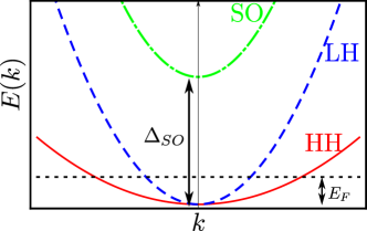
Figure 1: Sketch of energy dispersion of heavy hole, light hole and split-off bands for $p$-doped zinc-blende semiconductors.

Compound	$a$ (Å)	$\gamma_{1}$	$\gamma_{2}$	$\gamma_{3}$	$\gamma_{s}$	$\Delta_{SO}$ (eV)	$E_{F}$ (eV)
ZnTe	6.10	3.8	0.72	1.13	1.068	0.96	0.1195
GaAs	5.65	6.98	2.06	2.93	2.58	0.32-0.36	0.1377
GaP	5.45	4.05	0.49	2.93	1.95	0.03-0.13	0.01116

Table 1: Values of various parameters for the effective Luttinger Hamiltonian of families of zinc-blende semiconductors, from Ref. dietl-6x6 ; dietl0 ; review-jap . Typical hole density in these semiconductors varies between ($10^{24}-10^{26}$) m^-3. Here, we have taken the hole density $n_{h}=1.0\times 10^{26}$ m^-3 for all of them. It is clear from the table that for this typical order of density, the doubly degenerate two-band Hamiltonian is not applicable for GaAs and GaP , because $E_{F}$ is of the order of $\Delta_{SO}$. But for ZnTe, $E_{F}\ll\Delta_{SO}$ ($\Delta_{SO}\approx 8E_{F}$), so doubly degenerate two-band Luttinger Hamiltonian will be a good approximation. From now onwards we will only focus on ZnTe as an example to elaborate our results.

The above Hamiltonian $H_{0}$ is rotationally invariant and commutes with the helicity operator $\hat{\Lambda}={\bf k}\cdot{\bf J}/k$ so that its eigenvalues $\lambda=\pm 3/2,\pm 1/2$ are good quantum numbers. Here $\lambda=\pm 3/2$ and $\lambda=\pm 1/2$ correspond to the heavy hole and light hole states, respectively. Therefore, the eigenstates of the helicity operator are the same as the eigenstates of the Hamiltonian $H_{0}$. The energy dispersion of the heavy and light hole states are given by $E_{h/l}({\bf k})=(\hbar k)^{2}/(2m_{h/l})$ with $m_{h/l}=m_{0}/(\gamma_{1}\mp 2\gamma_{s})$ are the heavy and light hole masses, respectively. The two-fold degeneracy of heavy and light hole branches is due to the consequence of the space inversion and time-reversal symmetries of the Luttinger Hamiltonian. Using the basis of eigenstates of $J_{z}$, the eigenspinors $|\lambda,{\bf k}\rangle$ for $\lambda=3/2$ and $\lambda=1/2$ can be written as

$$|3/2,{\bf k}\rangle =\begin{pmatrix}\cos^{3}\frac{\theta}{2}e^{(-3i/2)\phi}\\ \sqrt{3}\cos^{2}\frac{\theta}{2}\sin\frac{\theta}{2}e^{(-i/2)\phi}\\ \sqrt{3}\cos\frac{\theta}{2}\sin^{2}\frac{\theta}{2}e^{(i/2)\phi}\\ \sin^{3}\frac{\theta}{2}e^{(3i/2)\phi}\end{pmatrix}$$ (6)

and

$$|1/2,{\bf k}\rangle =\begin{pmatrix}-\sqrt{3}\cos^{2}\frac{\theta}{2}\sin\frac{\theta}{2}e^{(-3i/2)\phi}\\ \cos\frac{\theta}{2}\Big{(}\cos^{2}\frac{\theta}{2}-2\sin^{2}\frac{\theta}{2}\Big{)}e^{(-i/2)\phi}\\ \sin\frac{\theta}{2}\Big{(}2\cos^{2}\frac{\theta}{2}-\sin^{2}\frac{\theta}{2}\Big{)}e^{(i/2)\phi}\\ \sqrt{3}\cos\frac{\theta}{2}\sin^{2}\frac{\theta}{2}e^{(3i/2)\phi}\end{pmatrix}.$$ (7)

The remaining spinors for $\lambda=-3/2$ and $\lambda=-1/2$ can easily be obtained from Eq. (6) and Eq. (7) under the spatial inversion operations $\theta\rightarrow\pi-\theta$ and $\phi\rightarrow\pi+\phi$.

Performing the standard procedure, the Fermi energy is given by

$$E_{F}=\frac{(\hbar{k_{\rm F}^{0e}})^{2}}{2m_{0}}\bigg{[}\frac{\gamma_{1}^{2}-4\gamma_{s}^{2}}{\big{[}(\gamma_{1}-2\gamma_{s})^{3/2}+(\gamma_{1}+2\gamma_{s})^{3/2}\big{]}^{2/3}}\bigg{]}$$ (8)

and the corresponding Fermi wave-vectors $k_{F}^{h/l}$ for heavy and light-hole bands, respectively, are given by

$$k_{F}^{h/l}=k_{\rm F}^{0e}\frac{m_{h/l}^{1/2}}{(m_{h}^{3/2}+m_{l}^{3/2})^{1/3}},$$ (9)

where $k_{F}^{0e}=(3\pi^{2}n_{h})^{1/3}$ with $n_{h}$ being the hole density. Also the density of states at Fermi energy is $\rho(E_{F})=(m_{h}^{3/2}+m_{l}^{3/2})^{2/3}k_{F}^{0e}/(\pi^{2}\hbar^{2})$. For a charge carrier with spin $s$ and carrier density $n_{c}$, we define $k_{F}^{0h/0e}=(\frac{6\pi^{2}n_{c}}{2s+1})^{1/3}$, where $s=3/2$ for hole gas and $s=1/2$ for electron gas, which implies $k_{F}^{0h}=k_{F}^{0e}/2^{1/3}$. Various parameters along with the Fermi energy for three different zinc blende semiconductors are given in Table I.

The Green function $G(\textbf{k},\omega+i0^{+})=[\omega+i0^{+}-H_{0}]^{-1}$ of the $4\times 4$ Luttinger Hamiltonian is then given by opt

$$G(\textbf{k},\omega) =\sum_{\lambda}\frac{1}{E_{\lambda}-\omega-i0^{+}}\begin{pmatrix}-\frac{1}{2}-\frac{\lambda(1+3\cos(2\theta))}{8}&-\frac{\lambda\sqrt{3}}{4}\sin(2\theta)e^{-i\phi}&-\frac{\lambda\sqrt{3}}{4}\sin^{2}\theta e^{-2i\phi}&0\\ -\frac{\lambda\sqrt{3}}{4}\sin(2\theta)e^{i\phi}&-\frac{1}{2}+\frac{\lambda(1+3\cos(2\theta))}{8}&0&-\frac{\lambda\sqrt{3}}{4}\sin^{2}\theta e^{-2i\phi}\\ -\frac{\lambda\sqrt{3}}{4}\sin^{2}\theta e^{2i\phi}&0&-\frac{1}{2}+\frac{\lambda(1+3\cos(2\theta))}{8}&\frac{\lambda\sqrt{3}}{4}\sin(2\theta)e^{-i\phi}\\ 0&-\frac{\lambda\sqrt{3}}{4}\sin^{2}\theta e^{2i\phi}&\frac{\lambda\sqrt{3}}{4}\sin(2\theta)e^{i\phi}&-\frac{1}{2}-\frac{\lambda(1+3\cos(2\theta))}{8}\end{pmatrix},$$ (10)

which we will use in the next section.

In these semiconductors, the magnetic impurities (Mn²⁺ state having localised $d$-orbitals) interact with each other by valance holes (having $p$-orbital) through the exchange interaction. So we assume $p$-$d$ type contact exchange interaction between the hole spin $\mathbf{J}(\mathbf{r})$ and the spins of the magnetic impurities $\mathbf{S}_{j}$, at positions $\mathbf{R}_{j}$ as

$$H_{p-d}=J_{pd}^{*}\sum_{j=1,2}\textbf{S}_{j}\cdot\textbf{J}(\mathbf{r})\hskip 4.2679pt\delta(\textbf{r}-\textbf{R}_{j})$$ (11)

with $J_{pd}^{*}$ is the strength of $p$-$d$ exchange interaction, whose dimension is energy times volume. Here $J_{pd}^{*}=J_{pd}/3$, with $J_{pd}=50$ eV $\r{A}^{3}$ for Mn doped ZnTe dilute magnetic semiconductorsdietl0 . Thus the total Hamiltonian of the system is $H=H_{0}+H_{p-d}$. By considering $H_{p-d}$ as a perturbation, the RKKY interaction is the second order correction to the ground state energy of $H_{0}$.

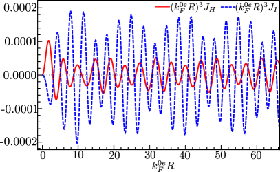
Figure 2: The range functions of RKKY interaction, from Eqs. 15 and 16, for Mn-doped ZnTe are plotted to show the beating pattern.

III RKKY interaction

The RKKY interaction between two impurity spins $\mathbf{S}_{1}$ and $\mathbf{S}_{2}$ put at a distance $\mathbf{R}$, at zero temperature, can be computed using second-order perturbation theory and it is expressed as follows

$$H_{{\rm RKKY}} = -\frac{J_{pd}^{2}}{9\pi}{\rm Im}\int_{-\infty}^{E_{F}}d\omega\hskip 2.84526pt{\rm Tr}[(\textbf{S}_{1}\cdot\textbf{J})\hskip 2.84526ptG(\textbf{R},\omega+i0^{+})$$ (12)

$$\times (\textbf{S}_{2}\cdot\textbf{J})\hskip 2.84526ptG(-\textbf{R},\omega+i0^{+})],$$

where ${\rm Tr}$ indicates a trace over the spin degree of freedom. The energy-coordinate representation of the Green’s function is given by

$$G(\pm\textbf{R},\omega+i0^{+})=\int\frac{d^{3}k}{(2\pi)^{3}}G(\textbf{k},\omega+i0^{+})e^{\pm i\textbf{k}\cdot\textbf{R}},$$ (13)

where we use the Green’s function as in Eq. (10). Without loss of generality, we consider the spins along the $z$ axis (i.e, $\mathbf{R}=R\hat{z}$) and after some tedious algebra, we obtain the RKKY interaction, containing only the Heisenberg and the Ising terms as

$$H_{\rm RKKY} = J_{H}\textbf{S}_{1}.\textbf{S}_{2}+J_{I}S_{1z}S_{2z},$$ (14)

where $J_{H}$ and $J_{I}$ denote range functions for the collinear Heisenberg and Ising terms, respectively. The non-collinear Dzyaloshinsky-Moriya (DM) dm1 ; dm2 coupling term is absent since the Luttinger Hamiltonian is invariant under spatial inversion. The detail derivation of $J_{H}$ and $J_{I}$ are given in the appendix, with the final form being

$$J_{H} =-\frac{J_{pd}^{2}}{(2\pi)^{3}}\Big{(}\frac{m_{h}}{9\hbar^{2}R^{4}}\Big{)}\Big{[}-\frac{9\cos(2\zeta^{h}_{F})}{2\zeta^{h}_{F}}-\Big{(}\frac{9\delta^{2}}{2\zeta^{l}_{F}}+2\delta^{2}\zeta^{l}_{F}\Big{)}\cos(2\zeta^{l}_{F})+\Big{(}-\frac{6\delta^{2}\zeta^{h}_{F}}{(1+\delta)}+\frac{9(1+\delta)}{2\zeta^{h}_{F}}\Big{)}\cos(\zeta^{h}_{F}+\zeta^{l}_{F})$$

$$+\Big{(}-\frac{9}{2}+\frac{9}{4(\zeta^{h}_{F})^{2}}\Big{)}\sin(2\zeta^{h}_{F})+\Big{(}\frac{5\delta^{2}}{2}+\frac{9\delta^{2}}{4(\zeta^{l}_{F})^{2}}\Big{)}\sin(2\zeta^{l}_{F})-\Big{(}\frac{9}{2(\zeta^{h}_{F})^{2}}+\frac{(3\delta^{3}-12\delta^{2}-9\delta)}{(1+\delta)^{2}}\Big{)}\sin(\zeta^{h}_{F}+\zeta^{l}_{F})$$

$$+\frac{9}{2}{\rm si}(2\zeta^{h}_{F})-\frac{15\delta^{2}}{2}{\rm si}(2\zeta^{l}_{F})+\Big{(}\frac{15\delta^{2}}{2}-\frac{9}{2}\Big{)}{\rm si}(\zeta^{h}_{F}+\zeta^{l}_{F})\Big{]},$$ (15)

$$J_{I} =-\frac{J_{pd}^{2}}{(2\pi)^{3}}\Big{(}\frac{3m_{h}}{18\hbar^{2}R^{4}}\Big{)}\Big{[}\Big{(}\frac{18}{\zeta_{F}^{h}}-3\zeta_{F}^{h}\Big{)}\cos(2\zeta^{h}_{F})+\Big{(}\frac{18\delta^{2}}{\zeta_{F}^{l}}+\delta^{2}\zeta_{F}^{l}\Big{)}\cos(2\zeta^{l}_{F})+\Big{(}\frac{4\delta^{2}\zeta_{F}^{h}}{1+\delta}-\frac{18(1+\delta)}{\zeta_{F}^{h}}\Big{)}\cos(\zeta_{F}^{h}+\zeta_{F}^{l})$$

$$+\Big{(}\frac{27}{2}-\frac{9}{(\zeta_{F}^{h})^{2}}\Big{)}\sin(2\zeta^{h}_{F})-\Big{(}\frac{\delta^{2}}{2}+\frac{9\delta^{2}}{(\zeta_{F}^{l})^{2}}\Big{)}\sin(2\zeta^{l}_{F})+\Big{(}\frac{18}{(\zeta_{F}^{h})^{2}}-\frac{4\delta(6+7\delta)}{(1+\delta)^{2}}\Big{)}\sin(\zeta_{F}^{h}+\zeta_{F}^{l})$$

$$-6{\rm si}(2\zeta^{h}_{F})+18\delta^{2}{\rm si}(2\zeta^{l}_{F})+6(1-3\delta^{2}){\rm si}(\zeta^{h}_{F}+\zeta^{l}_{F})\Big{]},$$ (16)

where, $\zeta^{\lambda}_{F}=k^{\lambda}_{F}R$ and $\delta=\sqrt{m_{l}/m_{h}}<1$ and ${\rm si}(x)=\int_{0}^{x}\frac{\sin t}{t}dt$ is the sine integral. It is evident from the above equations that the $J_{H}$ and $J_{I}$ oscillate with the distance between the spins, $R$, with multiple frequencies (due to the two different Fermi-wave vectors of the spin $s=3/2$ hole states), giving rise to beating pattern. The variation of $J_{H}$ and $J_{I}$ for a typical set of parameters has been plotted in Fig. 2. For large distances $J_{H}$ and $J_{I}$ (upto $1/R^{3}$ term) can be approximated as

$$J_{H} \simeq\frac{J_{pd}^{2}}{(2\pi)^{3}}\frac{2m_{h}\delta^{2}}{9\hbar^{2}R^{4}}\Big{[}\zeta^{l}_{F}\cos(2\zeta^{l}_{F})+\frac{3\zeta^{h}_{F}}{(1+\delta)}\cos(\zeta^{h}_{F}+\zeta^{l}_{F})\Big{]},$$ (17)

$$J_{I} \simeq\frac{J_{pd}^{2}}{(2\pi)^{3}}\frac{3m_{h}}{18\hbar^{2}R^{4}}\Big{[}3\zeta^{h}_{F}\cos(2\zeta^{h}_{F})-\delta^{2}\zeta^{l}_{F}\cos(2\zeta^{l}_{F})+\frac{4\delta^{2}}{(1+\delta)}\zeta^{h}_{F}\cos(\zeta^{h}_{F}+\zeta^{l}_{F})\Big{]}.$$ (18)

The nature of coupling (ferromagnetic/antiferromagnetic) between the magnetic impurities for a particular semiconductor is determined by the density of holes and the distance between the magnetic impurities.

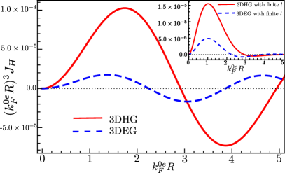
Figure 3: Comparison of the Heisenberg term of the RKKY interaction for Zn_1-xMn_xTe, calculated using 3DEG Hamiltonian with only one band together with different carrier mass ($m_{h}=0.5m_{0}$) and using the Luttinger Hamiltonian for 3DHG with two degenerate bands together with two different masses $m_{h}$ and $m_{l}$. Due to finite mean free path ($l$) of carriers, the response function decays exponentially. So we have also plotted in the inset of this figure the range function for the Heisenberg term with an exponential decay factor for $T_{C}$ calculation (see Eq. (21)). Due to this exponential decay, we require only few nearest neighbour distances ($k_{F}^{0e}R\approx$ upto $2$) to compute $T_{C}$. We have taken the mean free paths $l=0.65$ nm and $l=0.5$ nm for 3DEG case and 3DHG cases respectively.

The RKKY interaction of the hole doped semiconductors is different in nature from that of 3DEG, where such beating pattern is absent due to single band nature. The comparison of the two situations is plotted in Fig. 3. It can be easily checked that the Luttinger Hamiltonian reduces to that of the conventional 3DEG by setting $\gamma_{1}=1$ and $\gamma_{s}=0$. In this limit, $m_{h}=m_{l}=m_{0}$ and $k_{F}^{h}=k_{F}^{l}=k_{F}^{0h}$, the Ising-like range function exactly vanishes i.e, $J_{I}=0$ and the Heisenberg-like range function $J_{H}$ looks similar to the known form of the conventional 3DEG case diet ; rkkyanyD ,

$$J_{H} =-\frac{2J_{pd}^{2}(k_{F}^{0h})^{3}}{\pi}\tilde{\chi}_{h}\mathcal{F}(2k_{F}^{0h}R),$$ (19)

where $\mathcal{F}(y)=\frac{\sin(y)-y\cos(y)}{y^{4}}$ and $\tilde{\chi}_{h}=10m_{0}k_{F}^{0h}/36\pi^{2}\hbar^{2}$ is the static hole susceptibility. We have written above expression as a function of $k_{F}^{0h}$, because in the limiting situation $m_{l}=m_{h}$, we will have four degenerate bands.

IV Mean-field Curie-Weiss temperature

In this section, we will compute the contribution of the RKKY interaction to the Curie-Weiss temperature. In the mean-field approximation, the Curie-Weiss temperature $T_{c}$ is given by

$$k_{B}T_{C}=\frac{x}{3}S(S+1){J_{H}^{\rm eff}},$$ (20)

where $x$ is the magnetic dopant concentration, $S=5/2$ (for magnetic impurity Mn⁺² state) and spatial average of the Heisenberg-type response $J_{H}^{\rm eff}$ is given by

$${J_{H}^{\rm eff}}=\sum_{r}z_{r}J_{H}(r_{ij})e^{-r_{ij}/l}.$$ (21)

Here $z_{r}$ is the number of $r$-th neighbors (Ga-Ga), $l$ is carrier transport mean-free path which is introduced as an exponential factor in the effective interaction to take into account the fact that carriers can not pass the information from one magnetic impurity to other magnetic impurities which are situated at distances greater than the mean-free path of the carriers. We have used upto fourth nearest neighbour distances in the above summation, which is sufficient for Mn-doped ZnTe with mean-free path $l=0.5$ nm.

The origin of ferromagnetism in some dilute magnetic semiconductors is mostly due to the RKKY interaction mediated by valence holes. For these semiconductors, one can calculate $T_{C}$, using the given analytical form of $J_{H}$ with appropriate material parameters like mean free path of itinerant holes and strength of indirect exchange interaction $J_{pd}$, provided the density of holes is such that $E_{F}\ll\Delta_{SO}$. For higher hole densities, two-band approximation will not be valid and one has to take into account the contribution from the split-off band. Then we have to work with $6\times 6$ Kohn-Luttinger Hamiltonian, which will be more complicated. As mentioned in the Table I, for dilute magnetic semiconductors like (Ga,Mn)As, (Ga,Mn)P, our results will not be valid because for these systems hole density is such that Fermi energy becomes comparable with the split-off energy and then there will also be contribution from this band which is not included in our calculation. The critical temperature $T_{C}$ may also depend on other effects like hole-hole interaction, super-exchange etc dietl0 . For just an application of our analytical result, we present in Table II, the calculated $T_{C}$ of Mn-doped ZnTe dilute magnetic semiconductor for different magnetic dopant concentrations. For this material, we have taken mean free path exp-theory of the carrier holes $l=0.5$ nm and the strength of the exchange interaction exp-theory ; dietl-6x6 ; dietl0 $J_{pd}^{*}=50/3$ ${\rm eV\r{A}}^{3}$.

The RKKY interaction through the underlying Luttinger system is markedly different from a 3DEG system, although the resultant $T_{C}$ computed from either system may match closely. This is because of the small mean free path of the relevant semiconductors. The long range features such as the beating pattern do not have a strong contribution in $T_{C}$ as the range function is now multiplied by an exponentially decaying function, as shown in Fig. 3. This is the reason for successful prediction of the Curie-Weiss temperature in previous studies based in 3DEG modeling of these systems.

Mn-fraction	$T_{C}$
($x$)	(in Kelvin)
0.015	0.48
0.022	0.70
0.043	1.37
0.053	1.69
0.071	2.27

Table 2: Curie-Weiss temperature $T_{C}$ of dilute magnetic semiconductor (Zn,Mn)Te for various Mn-fraction $x$, which is calculated using Eq. (21). Experimental values of $T_{C}$: for Zn_1-xMn_xTe, $T_{C}\approx(1-10)$ K, for $x=(0.01-0.05)$ dietl-6x6 ; dietl0 .

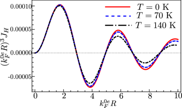
Figure 4: Temperature dependence of the RKKY interaction strength for Mn-doped ZnTe, showing the change in $J_{H}$ is small with the temperature for the distance between the impurities contributing to the mean-field $T_{C}$ calculation.

We have also computed the transition temperature $T_{C}$ using the temperature dependence of the RKKY interaction Maldague given by

$$J_{H}(E_{F},R,T)=\int_{-\infty}^{\infty}\frac{J_{H}(\omega,R)}{4k_{B}T\cosh^{2}((E_{F}-\omega)/2k_{B}T)}d\omega.$$

For the relevant parameters, $J_{H}(E_{F},R,T)$ depends weakly on the temperature, as shown in Fig. 4, for $R$ is of the order of the mean free path. Considering the spatial average $J_{H}^{\rm eff}(T)$, defined in equation Eq. (21), one solves Eq. 20 self-consistently to find the transition temperature $T_{c}$. As $J_{H}$ depends weakly on temperature for $R$ is of the order of mean free path, the resulting finite temperature estimation of $T_{C}$ does not differ significantly from what is presented in Table II.

V Summary and conclusions

In this work, we have studied RKKY interaction in Mn-doped bulk zinc-blende semiconductors, described by the $4\times 4$ Luttinger Hamiltonian. The analytical form of the interaction, as in Eqs. (15) and (16), describes the effect of the multiple bands through the presence of multiple frequency of oscillation giving rise to beating pattern in the range functions. For systems which are described by $4\times 4$ Luttinger Hamiltonian, we calculate the contribution of the RKKY interaction to the ferromagnetic transition temperature $T_{C}$. As an application of our analytical result, we have calculated $T_{C}$ for a zinc-blende semiconductor (Zn,Mn)Te. We also found that the spin-spin correlation is insensitive to temperature for small distances of the order of mean free path. Therefore finite temperature estimation of $T_{C}$ does not differ significantly from the estimation at $T=0$ K.

VI Acknowledgement

We would like to thank Tomasz Dietl and Joydeep Chakraborthy for useful discussion.

Appendix A Derivation of RKKY interaction

In this section we provide detail derivation of the RKKY interaction. For convenience, we choose ${\bf R}=R\hat{z}$ with $R=|{\bf R}_{1}-{\bf R}_{2}|$. It should be noted here that our results are the same for any arbitrary direction of ${\bf R}$. The Green’s function $G(\pm\textbf{R},\omega+i0^{+})$ is reduced to the following diagonal matrix:

$$G(\pm\textbf{R},\omega+i0^{+})=\begin{pmatrix}P_{0}&0&0&0\\ 0&Q_{0}&0&0\\ 0&0&Q_{0}&0\\ 0&0&0&P_{0}\end{pmatrix}.$$ (22)

Here the diagonal elements $P_{0}$ and $Q_{0}$ are expressed as $4P_{0}=-[I_{h}^{(1)}+3I_{h}^{(2)}+3I_{l}^{(1)}-3I_{l}^{(2)}]$ and $4Q_{0}=-[3I_{h}^{(1)}-3I_{h}^{(2)}+I_{l}^{(1)}+3I_{l}^{(2)}]$ with the integrals $I_{\lambda}^{(1)}$ and $I_{\lambda}^{(2)}$ are given by

$$I^{(1)}_{\lambda}=\int\frac{d^{3}k}{(2\pi)^{3}}\frac{e^{ikR\cos\theta}}{(E_{\lambda}-\omega-i0^{+})},$$ (23)

and

$$I^{(2)}_{\lambda}=\int\frac{d^{3}k}{(2\pi)^{3}}\frac{\cos^{2}\theta e^{ikR\cos\theta}}{(E_{\lambda}-\omega-i0^{+})}.$$ (24)

Considering $R>0$ and performing the three dimensional integrations, we obtain

$$I^{(1)}_{\lambda} = \frac{m_{\lambda}}{2\pi\hbar^{2}}\frac{e^{ik_{\lambda}R}}{R}$$ (25)

and

$$I^{(2)}_{\lambda} = \frac{m_{\lambda}}{\pi\hbar^{2}R}\Big{[}\frac{1}{k_{\lambda}^{2}R^{2}}+e^{ik_{\lambda}R}\Big{(}\frac{1}{2}+\frac{i}{k_{\lambda}R}-\frac{1}{k_{\lambda}^{2}R^{2}}\Big{)}\Big{]}$$ (26)

with $k_{\lambda}=\sqrt{2m_{\lambda}(\omega+i0^{+})/\hbar^{2}}$. The above expressions of $I^{(1)}_{\lambda}$ and $I^{(2)}_{\lambda}$ remains valid for $R<0$ as well. Now the final expressions for the components of the Green’s function are,

$$P_{0} = -\frac{m_{h}}{2\pi\hbar^{2}}\frac{e^{ik_{h}R}}{R}\Big{(}1+\frac{3i}{2k_{h}R}-\frac{3}{2k_{h}^{2}R^{2}}\Big{)}+\frac{3m_{l}}{4\pi\hbar^{2}}\frac{e^{ik_{l}R}}{R}\Big{(}\frac{i}{k_{l}R}-\frac{1}{k_{l}^{2}R^{2}}\Big{)}$$ (27)

and

$$Q_{0} = \frac{3m_{h}}{4\pi\hbar^{2}}\frac{e^{ik_{h}R}}{R}\Big{(}\frac{i}{k_{h}R}-\frac{1}{k_{h}^{2}R^{2}}\Big{)}-\frac{m_{l}}{2\pi\hbar^{2}}\frac{e^{ik_{l}R}}{R}\Big{(}1+\frac{3i}{2k_{h}R}-\frac{3}{2k_{h}^{2}R^{2}}\Big{)}.$$ (28)

Using Eq. (22), Eq. (12) can be reformulated as

$$H_{RKKY} = J_{H}{\bf S}_{1}\cdot{\bf S}_{2}+J_{I}S_{1z}S_{2z},$$ (29)

where the integral expressions of $J_{H}$ and $J_{I}$ are

$$J_{H} = -\frac{4J_{pd}^{2}}{9\pi}{\rm Im}\int_{-\infty}^{E_{f}}Q_{0}(3P_{0}+2Q_{0})d\omega$$ (30)

$$J_{I} = -\frac{6J_{pd}^{2}}{9\pi}{\rm Im}\int_{-\infty}^{E_{f}}(3P_{0}^{2}-Q_{0}^{2}-2P_{0}Q_{0})d\omega.$$ (31)

Using Eqs. (27) and (28) into tne integral expressions of the range functions $J_{H}$ and $J_{I}$ and performing the energy integral, the exact analytical expressions of the range functions are

$$J_{H} = -\frac{J_{pd}^{2}}{(2\pi)^{3}}\Big{(}\frac{m_{h}}{9\hbar^{2}R^{4}}\Big{)}\Big{[}-\frac{9\cos(2\zeta^{h}_{F})}{2\zeta^{h}_{F}}-\Big{(}\frac{9\delta^{2}}{2\zeta^{l}_{F}}+2\delta^{2}\zeta^{l}_{F}\Big{)}\cos(2\zeta^{l}_{F})+\Big{(}-\frac{6\delta^{2}\zeta^{h}_{F}}{(1+\delta)}+\frac{9(1+\delta)}{2\zeta^{h}_{F}}\Big{)}\cos(\zeta^{h}_{F}+\zeta^{l}_{F})$$ (32)

$$+ \Big{(}-\frac{9}{2}+\frac{9}{4(\zeta^{h}_{F})^{2}}\Big{)}\sin(2\zeta^{h}_{F})+\Big{(}\frac{5\delta^{2}}{2}+\frac{9\delta^{2}}{4(\zeta^{l}_{F})^{2}}\Big{)}\sin(2\zeta^{l}_{F})-\Big{(}\frac{9}{2(\zeta^{h}_{F})^{2}}+\frac{(3\delta^{3}-12\delta^{2}-9\delta)}{(1+\delta)^{2}}\Big{)}\sin(\zeta^{h}_{F}+\zeta^{l}_{F})$$

$$+ \frac{9}{2}{\rm si}(2\zeta^{h}_{F})-\frac{15\delta^{2}}{2}{\rm si}(2\zeta^{l}_{F})+\Big{(}\frac{15\delta^{2}}{2}-\frac{9}{2}\Big{)}{\rm si}(\zeta^{h}_{F}+\zeta^{l}_{F})\Big{]},$$

$$J_{I} = -\frac{J_{pd}^{2}}{(2\pi)^{3}}\Big{(}\frac{3m_{h}}{18\hbar^{2}R^{4}}\Big{)}\Big{[}\Big{(}\frac{18}{\zeta_{F}^{h}}-3\zeta_{F}^{h}\Big{)}\cos(2\zeta^{h}_{F})+\Big{(}\frac{18\delta^{2}}{\zeta_{F}^{l}}+\delta^{2}\zeta_{F}^{l}\Big{)}\cos(2\zeta^{l}_{F})+\Big{(}\frac{4\delta^{2}\zeta_{F}^{h}}{1+\delta}-\frac{18(1+\delta)}{\zeta_{F}^{h}}\Big{)}\cos(\zeta_{F}^{h}+\zeta_{F}^{l})$$ (33)

$$+ \Big{(}\frac{27}{2}-\frac{9}{(\zeta_{F}^{h})^{2}}\Big{)}\sin(2\zeta^{h}_{F})-\Big{(}\frac{\delta^{2}}{2}+\frac{9\delta^{2}}{(\zeta_{F}^{l})^{2}}\Big{)}\sin(2\zeta^{l}_{F})+\Big{(}\frac{18}{(\zeta_{F}^{h})^{2}}-\frac{4\delta(6+7\delta)}{(1+\delta)^{2}}\Big{)}\sin(\zeta_{F}^{h}+\zeta_{F}^{l})$$

$$- 6{\rm si}(2\zeta^{h}_{F})+18\delta^{2}{\rm si}(2\zeta^{l}_{F})+6(1-3\delta^{2}){\rm si}(\zeta^{h}_{F}+\zeta^{l}_{F})\Big{]}.$$

Here, ${\rm si}(x)=\int_{0}^{x}\frac{\sin t}{t}dt$ is the sine integral.

Appendix B Derivation of static spin susceptibility

Following Ref.dietl0 , the longitudinal static spin susceptibility for this system can be written as

$$\chi({\bf q},\mu,T)=\frac{1}{9V}\sum_{\lambda_{1},\lambda_{2},{\bf k}}|\langle\lambda_{1},{\bf k}|J_{z}|\lambda_{2},{\bf k}+{\bf q}\rangle|^{2}\frac{f(\lambda_{1},{\bf k})-f(\lambda_{2},{\bf k}+{\bf q})}{E_{\lambda_{2}}({\bf k}+{\bf q})-E_{\lambda_{1}}({\bf k})},$$ (34)

where $|\lambda,{\bf k}\rangle$ is the eigen spinor of the Hamiltonian with eigen energy $E_{\lambda}({\bf k})$ defined in the main text, $f(\lambda,{\bf k})=1/(\exp(\beta(E_{\lambda}({\bf k})-\mu))+1)$ is the Fermi-Dirac distribution function with $\beta=1/k_{B}T$ and $\mu$ being the chemical potential. We calculate the static spin susceptibility at zero temperature for hole gas by separating out the intraband and interband contributions as $\chi_{h}(0)=\chi_{\rm intra}(E_{F})+\chi_{\rm inter}(E_{F})$. After some straight forward steps from Eq. (34), we get

$$\chi_{\rm intra}(E_{F})=\frac{1}{9V}\sum_{\lambda,{\bf k}}|\langle\lambda_{1},{\bf k}|J_{z}|\lambda_{2},{\bf k}\rangle|^{2}\delta(E_{\lambda}({\bf k})-E_{F})$$ (35)

and

$$\chi_{\rm inter}(E_{F})=\frac{1}{9V}\sum_{\lambda_{1}\neq\lambda_{2},{\bf k}}|\langle\lambda_{1},{\bf k}|J_{z}|\lambda_{2},{\bf k}\rangle|^{2}\frac{\Theta(E_{F}-E_{\lambda_{1}}({\bf k}))-\Theta(E_{F}-E_{\lambda_{2}}({\bf k}))}{E_{\lambda_{2}}({\bf k})-E_{\lambda_{1}}({\bf k})}.$$ (36)

The intraband and interband matrix elements $\langle\lambda_{1},{\bf k}|J_{z}|\lambda_{2},{\bf k}\rangle$ in terms of polar angle $\theta$ of ${\bf k}$ are as folllows: $\langle\lambda,{\bf k}|J_{z}|\lambda,{\bf k}\rangle=\lambda\cos\theta,\langle\pm 1/2,{\bf k}|J_{z}|\mp 1/2,{\bf k}\rangle=-\sin\theta,\langle\pm 3/2,{\bf k}|J_{z}|\pm 1/2,{\bf k}\rangle=-(\sqrt{3}/2)\sin\theta,\langle\pm 1/2,{\bf k}|J_{z}|\pm 3/2,{\bf k}\rangle=-(\sqrt{3}/2)\sin\theta,\langle\pm 3/2,{\bf k}|J_{z}|\mp 3/2,{\bf k}\rangle=0,\langle\pm 1/2,{\bf k}|J_{z}|\mp 3/2,{\bf k}\rangle=0$, and $\langle\pm 3/2,{\bf k}|J_{z}|\mp 1/2,{\bf k}\rangle=0$.

We calculate the static spin susceptibility using the above matrix elements in Eqs. (35) and (36). For intraband contribution to static spin susceptibility $\chi_{\rm intra}(E_{F})=\chi_{\frac{1}{2}}(E_{F})+\chi_{\frac{3}{2}}(E_{F})$, where contribution from light hole band $\chi_{1/2}(E_{F})$ and heavy hole band $\chi_{3/2}(E_{F})$ are obtained as $\chi_{\frac{1}{2}}(E_{F})=\frac{3m_{l}k_{F}^{l}}{36\pi^{2}\hbar^{2}}$ and $\chi_{\frac{3}{2}}(E_{F})=\frac{3m_{h}k_{F}^{h}}{36\pi^{2}\hbar^{2}}$. For interband contribution, $\chi_{\rm inter}(E_{F})=\chi_{\frac{1}{2},\frac{3}{2}}(E_{F})+\chi_{\frac{3}{2},\frac{1}{2}}(E_{F})$, where

$$\chi_{\frac{1}{2},\frac{3}{2}}(E_{F})=\chi_{\frac{3}{2},\frac{1}{2}}(E_{F})=\frac{1}{9\pi^{2}\hbar^{2}}\frac{(k_{F}^{h}-k_{F}^{l})m_{h}m_{l}}{m_{h}-m_{l}}.$$ (37)

Using the expressions of the heavy and light hole Fermi wave vectors $k_{F}^{h/l}$ given in Eq. (9), the final form of total static spin susceptibility isdietl0

$$\chi_{h}(0) =\frac{1}{4}\rho(E_{F})\Big{[}\frac{1}{3}+\frac{8}{9}\frac{(m_{h}^{3/2}m_{l}-m_{l}^{3/2}m_{h})}{(m_{h}-m_{l})(m_{h}^{3/2}+m_{l}^{3/2})}\Big{]}.$$ (38)

Here $\rho(E_{F})=(m_{h}^{3/2}+m_{l}^{3/2})^{2/3}k_{F}^{0e}/(\pi^{2}\hbar^{2})$ is the density of states at the Fermi energy.

Appendix C Limiting case

The Luttinger Hamiltonian reduces to the Hamiltonian of a 3DHG with four degenerate bands by setting $\gamma_{1}=1$ and $\gamma_{s}=0$. In this limit, the static hole spin susceptibility calculated from Eq. (38) is

$$\tilde{\chi}_{h}=\frac{10m_{0}k_{F}^{0h}}{36\pi^{2}\hbar^{2}}.$$ (39)

Similarly, setting $\gamma_{1}=1$ and $\gamma_{s}=0$ in Eqs. 32 and 33, the Ising-like range function exactly vanishes i.e . $J_{I}=0$ and the Heisenberg-like range function $J_{H}$ becomes

$$J_{H} =-\frac{2J_{pd}^{2}(k_{F}^{0h})^{3}}{\pi}\tilde{\chi}_{h}\mathcal{F}(2k_{F}^{0h}R),$$ (40)

where $\mathcal{F}(y)=\frac{\sin(y)-y\cos(y)}{y^{4}}$. On the other hand, the analytical form of the RKKY interaction for conventional 3DEG with two degenerate bands is given by diet

$$J_{H} =-\frac{2J_{sd}^{2}(k_{F}^{0e})^{3}}{\pi}\tilde{\chi}_{e}\mathcal{F}(2k_{F}^{0e}R),$$ (41)

where $\tilde{\chi}_{e}=m_{0}k_{F}^{0e}/(4\pi^{2}\hbar^{2})$ is the static electron spin susceptibility. So we see from Eqs. (40) and (41) that similar relation between RKKY interaction and static spin susceptibility follows for both the cases.

References

- (1) S. Murakami, N. Nagaosa, and S. C. Zhang, Science 301, 1348 (2003).
- (2) J. M. Luttinger, Phys. Rev. 102, 1030 (1956).
- (3) Y. K. Kato, R. C. Myers, A. C. Gossard, and D. D. Awschalom, Science 306, 1910 (2004).
- (4) J. Wunderlich, B. Kaestner, J. Sinova, and T. Jungwirth, Phys. Rev. Lett. 94, 047204 (2005).
- (5) M. W. Wu, J. H. Jiang, and M. Q. Weng, Physics Reports 493, 61 (2010).
- (6) J. Schliemann, A. Khaetskii, and D. Loss, J. Phys.: Condens. Matt. 15, R1809 (2003).
- (7) T. Korn, M. Kugler, M. Griesbeck, R. Schulz, A. Wagner, M. Hirmer, C. Gerl, D. Schuh, W. Wegscheider, and C. Schuller, New J. Phys. 12, 043003 (2010).
- (8) M. Kugler, T. Andlauer, T. Korn, A. Wagner, S. Fehringer, R. Schulz, M. Kubova, C. Gerl, D. Schuh, W. Wegscheider, P. Vogl, and C. Schuller, Phys. Rev. B 80, 035325 (2009).
- (9) S. Murakami, N. Nagaosa, and S. C. Zhang, Phys. Rev. B 69, 235206 (2004).
- (10) Z. F. Jiang, R. D. Li, S.-C. Zhang, and W. M. Liu, Phys. Rev. B 72, 045201 (2005).
- (11) R. Winkler, U. Zulicke, and J. Bolte, Phys. Rev. B 75, 205314 (2007).
- (12) V. Ya. Demikhovskii, G. M. Maksimova, and E. V. Frolova, Phys. Rev. B 81, 115206 (2010).
- (13) J. Schliemann, Phys. Rev. B 74, 045214 (2006).
- (14) J. Schliemann, Euro. Phys. Lett 91, 67004 (2010).
- (15) J. Schliemann, Phys. Rev. B 84, 155201 (2011).
- (16) Jun-Won Rhim and Y. B. Kim, Phys. Rev. B 91, 115124 (2015).
- (17) A. Mawrie, P. Halder, B. Ghosh, and T. K. Ghosh, J. Appl. Phys. 120, 124309 (2016).
- (18) M. A. Ruderman and C. Kittel, Phys. Rev. 96, 99 (1954).
- (19) T. Kasuya, Prog. Theor. Phys. 16, 45 (1956).
- (20) K. Yosida, Phys. Rev. 106, 893 (1957).
- (21) S. S. P. Parkin, N. More, and K. P. Roche, Phys. Rev. Lett. 64, 2304 (1990).
- (22) A. Manchon, H. C. Koo, J. Nitta, S. M. Frolov, and R. A. Duine, Nat. Matter. 14, 871 (2015).
- (23) H. Imamura, P. Bruno, and Y. Utsumi, Phys. Rev. B 69, 121303 (2004).
- (24) A. Schulz, A. De Martino, P. Ingenhoven, R. Egger, Phys. Rev. B 79, 205432 (2009).
- (25) J.-J. Zhu, K. Chang, R.-B. Liu, and H.-Q. Lin, Phys. Rev. B 81, 113302 (2010).
- (26) J. Klinovaja and D. Loss, Phys. Rev. B 87, 045422 (2013).
- (27) P. Lyu, N.-N. Liu, and C. Zhang, S.-X Wang, H. R. Chang, and J. Zhou, J. Appl. Phys. 102, 103910 (2007).
- (28) P. Simon, B. Braunecker, and D. Loss, Phys. Rev. B 77, 045108 (2008).
- (29) T. Kernreiter, Phys. Rev. B 88, 085417 (2013).
- (30) H. Min, E. H. Hwang, and S. Das Sarma, Phys. Rev. B 95, 155414 (2017).
- (31) S. Verma and A. Kundu, Phys. Rev. B 99, 121409(R) (2019).
- (32) SK Firoz Islam, P. Dutta, A. M. Jayannavar, and A. Saha, Phys. Rev. B 97, 235424 (2018).
- (33) S.-X Wang, H. R. Chang, and J. Zhou, Phys. Rev. B 96, 115204 (2017).
- (34) H. Munekata, H. Ohno, S. von Molnár, A. Segmüller, L. L. Chang, and L. Esaki, Phys. Rev. Lett. 63, 1849 (1989).
- (35) H. Ohno, Science 281, 951 (1998); T. Hayashi, Y. Hashimoto, S. Katsumoto, and Y. Iye, Appl. Phys. Lett. 78, 1691 (2001).
- (36) Y. Nagai, T. Kunimoto, K. Nagasaka, H. Nojiri, M. Motokawa, F. Matsukura, T. Dietl, and H. Ohno, Jpn. J. Appl. Phys. 40, 6231 (2001).
- (37) S. Katsumoto, T. Hayashi, Y. Hashimoto, Y. Iye, Y. Ishiwata, M. Watanabe, R. Eguchi, T. Takeuchi, Y. Harada, and S. Shin, Mater. Sci. Eng., B 84, 88 (2001).
- (38) K. Hirakawa, S. Katsumoto, T. Hayashi, Y. Hashimoto, and Y. Iye, Phys. Rev. B 65, 193312 (2002).
- (39) K. W. Edmonds, P. Boguslawski, K. Y. Wang, R. P. Campion, S. N. Novikov, N. R. S. Farley, B. L. Gallagher, C. T. Foxon, M. Sawicki, T. Dietl, M. Buongiorno Nardelli, and J. Bernholc, Phys. Rev. Lett. 92, 037201, (2004).
- (40) T. Jungwirth, K. Y. Wang, J. Masek, K. W. Edmonds, J. Konig, J. Sinova, M. Polini, N. A. Goncharuk, A. H. MacDonald, M. Sawicki, A.W. Rushforth, R. P. Campion, L. X. Zhao, C. T. Foxon, and B. L. Gallagher, Phys. Rev. B 72, 165204 (2005).
- (41) F. Matsukura, H. Ohno, A. Shen, and Y. Sugawara, Phys. Rev. B 57, R2037 (1998).
- (42) T. Dietl, Semicond. Sci. Technol. 17, 377 (2002); T. Jungwirth, J. Sinova, J. Masek, J. Kucera, and A. H. MacDonald, Rev. Mod. Phys. 78, 809, (2006); T. Dietl and H. Ohno, Rev. Mod. Phys. 86, 187, (2014).
- (43) A. X. Gray, J. Minar, S. Ueda, P. R. Stone, Y. Yamashita, J. Fujii, J. Braun, L. Plucinski, C. M. Schneider, G. Panaccione, H. Ebert, O. D. Dubon, K. Kobayashi, and C. S. Fadley, Nat Mater. 11, 957 (2012).
- (44) M. A. Scarpulla, B. L. Cardozo, R. Farshchi, W. M. Hlaing Oo, M. D. McCluskey, K. M. Yu, and O. D. Dubon, Phys. Rev. Lett. 95, 207204 (2005).
- (45) A. Keqi, M. Gehlmann, G. Conti, S. Nemsak, A. Rattanachata, J. Minar, L. Plucinski, J. E. Rault, J. P. Rueff, M. Scarpulla, M. Hategan, G. K. Palsson, C. Conlon, D. Eiteneer, A. Y. Saw, A. X. Gray, K. Kobayashi, S. Ueda, O. D. Dubon, C. M. Schneider, and C. S. Fadley, Phys. Rev. B 97, 155149 (2018).
- (46) T. Dietl, H. Ohno, F. Matsukura, J. Cibert, and D. Ferrand, Science 287, 1019 (2000); T. Dietl, H. Ohno, and F. Matsukura, Phys. Rev. B 63, 195205 (2001).
- (47) M. Berciu and R. N. Bhatt, Phys. Rev. Lett. 87, 107203 (2001); A. L. Chudnovskiy and D. Pfannkuche, Phys. Rev. B 65, 165216 (2002); G. A. Fiete, G. Zaránd, and K. Damle, Phys. Rev. Lett. 91, 097202 (2003).
- (48) A. C. Durst, R. N. Bhatt, and P. A. Wolff, Phys. Rev. B 65, 235205 (2002); A. Kaminski and S. Das Sarma, Phys. Rev. Lett. 88, 247202 (2002).
- (49) V. I. Litvinov and V. K. Dugaev, Phys. Rev. Lett. 86, 5593 (2001).
- (50) T. Dietl, H. Ohno, and F. Matsukura, Phys. Rev. B 63, 195205 (2001); M. Abolfath, T. Jungwirth, J. Brum, and A. H. MacDonald, Phys. Rev. B 63, 054418 (2001).
- (51) D. Ferrand, J. Cibert, A. Wasiela, C. Bourgognon, S. Tatarenko, G. Fishman, T. Andrearczyk, J. Jaroszynski, S. Kolesnik, T. Dietl, B. Barbara, and D. Dufe, Phys. Rev. B 63, 085201 (2001).
- (52) T. Dietl, A. Haury and Y. Merle d’Aubigne, Phys. Rev. B 55, R3347 (1997).
- (53) D. N. Aristov, Phys. Rev. B 55, 8064 (1997).
- (54) A. Singh, A. Datta, S. K. Das, and V. A. Singh, Phys. Rev. B 68, 235208 (2003).
- (55) C. Timm and A. H. MacDonald, Phys. Rev. B 71, 155206 (2005).
- (56) J. M. Luttinger and W. Kohn, Phys. Rev. 97, 869 (1955).
- (57) A. Baldereschi and N. O. Lipari, Phys. Rev. B 8, 2697 (1973); M. Altarelli, U. Ekenberg, and A. Fasolino, Phys. Rev. B 32, 5138 (1985).
- (58) I. Vurgaftman, J. R. Meyer, and L. R. Ram-Mohan, J. App. Phys. 89, 5815 (2001).
- (59) I. Dzyaloshinsky, J. Phys. Chem. Solids 4, 241 (1958).
- (60) T. Moriya, Phys. Rev. 120, 91 (1960).
- (61) P. F. Maldague, Surf. Sci. 73, 296 (1978).