Exact Master Equation and General Non-Markovian Dynamics
in Open Quantum Systems

Abstract

Investigations of quantum and mesoscopic thermodynamics force one to answer two fundamental questions associated with the foundations of statistical mechanics: (i) how does macroscopic irreversibility emerge from microscopic reversibility? (ii) how does the system relax in general to thermal equilibrium with its environment? The answers to these questions rely on a deep understanding of nonequilibrium dynamics of systems interacting with their environments. Decoherence is also a main concern in developing quantum information technology. In the past two decades, many theoretical and experimental investigations have devoted to this topic, most of these investigations take the Markov (memory-less) approximation. These investigations have provided a partial understanding to several fundamental issues, such as quantum measurement and the quantum-to-classical transition, etc. However, experimental implementations of nanoscale solid-state quantum information processing makes strong non-Markovian memory effects unavoidable, thus rendering their study a pressing and vital issue. Through the rigorous derivation of the exact master equation and a systematical exploration of various non-Markovian processes for a large class of open quantum systems, we find that decoherence manifests unexpected complexities. We demonstrate these general non-Markovian dynamics manifested in different open quantum systems.

I Introduction

As it is well-known, any realistic system will inevitably interact with its environment. For nano-scale quantum devices or more general mesoscopic systems, such interactions are usually not negligible, and thus these objects must be treated as open systems. Specifically, an open system is defined as the principal system consisting of only a few relevant dynamical variables in contact with an environment containing a huge (infinite) number of degrees of freedom. Understanding the dynamics of open systems is also one of the most challenging topics in physics, chemistry, biology and even engineering. In particular, the interactions between the principal system and the environment can induce various back-reactions between them such that the system can memory its historical evolution. These memory processes are characterized as the non-Markovian dynamics in open systems, to distinguish from the memoryless processes which are named as Markov dynamics in the literature.

Physically, non-Markovian dynamics can be described by different time correlations associated with environment-induced dissipation and fluctuation dynamics in open systems. To understand the quantum dynamics of open systems, many different approaches were developed. In principle, the system we care about plus its environments together form a closed system, which is governed by the Schrödinger equation in terms of the wave function of the total system or the von Neumann equation in terms of the total density matrix. Usually the environment is assumed to be initially in a thermal equilibrium state at a given temperature $T$, which is a mixed state. Thus, the Schrödinger picture is no longer applicable. One has to use the von Neumann equation in terms of the density matrix to solve the dynamics of the total system. The solution of the density matrix contains all predictions to various physical observables.

Practically, it is very difficult to solve the von Neumann equation of the total system, due to the infinite number of degrees of freedom involved in the environment. More important, we are only interested in the dynamics of the principal system itself, rather than the dynamics of its environment. Hence, for a long time, a central issue in the investigations of the dynamics of open system has been focused on finding the equation of motion for the reduced density matrix of the principal system. Such an equation of motion is called as Master Equation. Within the framework of von Neumann equation of the total system, the master equation can be derived in principle from quantum mechanics, as I will attempt to do so in this article. On the other hand, from the open system point of view, the master equation actually plays an even more important role for the foundation of statistical mechanics Huang87 , in comparison with the Newtonian equation for macroscopic objects, the Maxwell equations for electrodynamics, and the Schrödinger equation for isolated quantum systems. From the more fundamental point of view, the Newtonian equation can be derived from the Lagrangian formalism, the Maxwell equations can be derived from the field theory of quantum electrodynamics (QED), and the Schrödinger equation is only a nonrelativistic approximation of the Dirac equation which can also be derived from QED, while it is not clear if there is a fundamental principle to directly determine the master equation. With this aspect, finding the master equation for open quantum systems is a big challenge in science. Certainly, if one can find the exact master equation for arbitrary open systems, many interesting and fundamental problems in open system dynamics, including non-Markovian memory dynamics I will focus on this in article, can be easily addressed.

Historically, the first master equation was phenomenologically introduced by Pauli in 1928 Pauli , which is now called the Pauli master equation in the literature. In the past many decades, one has made progresses with various approaches in deriving the master equation for different open quantum systems. These include the Nakajawa-Zeneng master equation Nakajima ; Zwanzig , the Born or Born-Markov master equation Hove ; Haake , the GKS-Lindblad master equation GKS ; Lindblad , etc. However, all these master equations are either practically unsolvable Nakajima ; Zwanzig or only applicable for Markov dynamics Hove ; Haake ; GKS ; Lindblad . Until 1980’s, Caldeira and Leggett systematically derived a master equation for quantum Brownian motion Caldeira1983 , using the Feynman-Vernon influence functional approach Fey1963 to explicitly and exactly integrate out all the environment degrees of freedom. Since then, the quantum Brownian motion becomes a prototype example in understanding the dynamics of open quantum systems Weiss08 . In reality, however, no many systems can be treated with the quantum Brownian motion. There is still a lack of satisfactory answer to the master equation and to open quantum system dynamics in general. Indeed, not having a rigorous and more general master equation for a large class of realistic open quantum systems remains a primary obstacle in understanding many fundamental problems in physics.

To address physically the more general essence of open quantum system dynamics, we developed a full non-Markovian decoherence theory PRL2012 ; PRB2008 ; NJP2010 ; ANNP2012 ; PRB2015 ; PRB18 with the exact master equation we derived recently for a class of open systems. These open systems linearly couple to environments but are different from the quantum Brownian motion. More specifically, the system and the environments are described with Fano-Anderson type Hamiltonians Anderson1961 ; Fano1961 that have wide applications in atomic physics, quantum optics, condensed matter physics and particle physics Tannoudji92 ; Lam00 ; Mahan2000 . Here both the system and the environment can be either bosonic or fermionic, and it may also be extendible to spin-like systems. We find PRL2012 ; PRB2008 ; NJP2010 ; ANNP2012 ; PRB2015 ; PRB18 that the dissipation and fluctuations coefficients in our exact master equation are intimately connected with nonequilibrium Green functions in many-body systems Schwinger1961 ; Keldysh1965 ; Kadanoff1962 . As a result, we show that the nonequilibrium Green functions that obey the integro-differential convolution equations depict all possible non-Markovian memory dynamics through the time-convolution integral structures PRL2012 ; Xiong2010 ; Sci2015b ; Sci2015a ; PRA2015 ; Lei2011 ; Ali2017 .

I should emphasize from the very beginning that in the reality, non-Markovian dynamics is well-defined as memory processes in open systems. Experimentally, non-Markovian dynamics can be quantified though direct measurements of two-time correlation functions which demonstrate explicitly memory effects. The fundamental study of quantum dynamics and the technology development of quantum information processing show that it is crucially important to understand general physical behaviors of non-Markovian dynamics, namely how different energy structures of the system and the environment, and different couplings between them, including different initial state dependences on the system and the environment, determine different memory effects of open quantum systems. Such understanding could truly help one to engineeringly control and manipulate decoherence in practical applications in quantum technology, and therefore it is my main concern in the study of non-Markovian dynamics in open quantum systems.

It may also be worth pointing out that the study of non-Markovian decoherence dynamics in open quantum systems has attracted a great deal of attentions recently Vega2017 . Most of investigations have been focused on how to mathematically quantify the degree of non-Markovianity by introducing different concepts, such as divisibility Wolf2008 ; Rivas2010 and distinguishability of states Breuer09 , etc., in an attempt of mathematically characterizing quantum Markovianity. The results from these investigations are much definition-dependent and the conclusions often diverge from each other. It is therefore not the topic I will discuss in this article.

II Structures of system-environment couplings

Undoubtedly, dynamics of open quantum systems crucially depend on the structure of system-environment couplings or interactions. Here I would like to begin with a discussion on possible system-environment couplings we may encounter in practical applications.

A general open quantum system is defined as a principal system of interest interacting with its surroundings as its environments (or reservoirs). The interactions between the system and its environments are the manifestation of the exchanges of matters, energies and informations between them. A general Hamiltonian describing the coupling between the system and its environments can be formally written as

$$H=H_{S}+H_{E}+H_{\rm SE},$$ (1)

where $H_{S}$ and $H_{E}$ are the Hamiltonians of the system and the environment, respectively, and $H_{SE}$ denotes the interaction between them. The explicit form of $H_{SE}$ depends on the particular system and its environment(s) that we concern.

The simplest realization of such an open quantum system was originally introduced by Feynman and Vernon in the seminal paper in 1963 Fey1963 , where Feynman and Vernon developed a theory named influence functional, based on the path-integral formalism Fey65 , to deal with the influence of linear environmental systems acting on the principal system. In particular, they modeled the linear environmental systems as a sum of an infinite number of harmonic oscillators. In 1980s, Caldeira and Leggett used the approach of Feynman-Vernon influence functional to study in details the dynamics of a Brownian particle under the influence of such an environment Caldeira1983 , which is now called as the Caldeira-Leggett (CL) model in the literature. The significance of the CL model is the emergence of the classical dissipation motion of a Brownian particle within the framework of quantum mechanics. The equilibrium fluctuation-dissipation theorem proposed originally by Einstein is also naturally obtained quantum mechanically from this model. Thus, the CL model becomes a prototype model in the study of the dynamics of open quantum systems Weiss08 .

On the other hand, the rapid developments of new emerging research fields on nano technologies and quantum information sciences have stimulated tremendous interests on decoherence dynamics of tiny quantum devices, due to their invertible interaction with various environments surrounding. Typical examples include semiconductor nanostructures in mesoscopic physics, nanophotonics in photonic crystals and metamaterials, nanostructured cavity QED, and electrons or nuclear spins interacting with a thermal spin bath, just to name a few. These open quantum systems, which are currently very popular in the practical applications of nanotechnologies and quantum information sciences, go much beyond the Caldeira-Leggett model of the quantum Brownian motion. The general Hamiltonian for these system-environment couplings should be analyzed physically in a more realistic manner, as I will discuss in the following.

Consider first the exchange of matters between the system and its environments. Since matters are built with fermions, i.e. electrons and nuclei (or more fundamentally, quarks), we should start with both the system and its environments being made of fermions. Let $a_{i},a^{\dagger}_{i}$ and $b_{\alpha k},b^{\dagger}_{\alpha k}$ denote the creation and annihilation operators of fermions of the system and the environment $\alpha$, respectively, which satisfy the standard fermionic anti-commutation relationships. Then the most basic process for the underlying matter exchange between the system and its environments can be described effectively through the following Hamiltonian:

$$H(t)= \sum_{i}\varepsilon_{ij}(t)a^{\dagger}_{i}a_{j}+\sum_{\alpha k}\epsilon_{\alpha k}(t)b^{\dagger}_{\alpha k}b_{\alpha k}+\sum_{\alpha ik}\Big{(}V_{i\alpha k}(t)a^{\dagger}_{i}b_{\alpha k}+V^{*}_{i\alpha k}(t)b^{\dagger}_{\alpha k}a_{i}\Big{)},$$ (2)

where the system-environment coupling, i.e. the last term in the above equation, is realized through particle tunnelings between the system and its environments. The index $\alpha$ denotes different environments in contact with the same systems. I let all the parameters in the Hamiltonian be time-dependent because current nanotechnologies are capable to tune these parameters effectively through various external fields, such as bias and gate voltages in nanoelectronics. The form of Eq. (2) is indeed a generalized Fano-Anderson Hamiltonian in condensed matter physics Mahan2000 , as it was originally introduced by Anderson Anderson1961 and Fano Fano1961 independently, to describe impurity electrons coupled to continuous states in solid-state physics, and discrete states embedded in a continuum in atomic spectra, respectively. In the past two decades, one has started with such Hamiltonians to investigate various electron transport phenomena and decoherence dynamics in semiconductor nanoelectronics and spintronics for mesoscopic physics, where the nano-scale electron system is in contact with two (or more) electrodes which serve as the electronic reservoirs Hang1996 ; Imry2002 .

The system interacting with its environments in terms of the Fano-Anderson Hamiltonian (2) has also been applied to the case where both the system and the environments are made of bosons as composite particles of fermions, such as atoms that Fano originally proposed Fano1961 , or more fundamentally made of scalar fields Lee1954 . Correspondingly, the creation and annihilation operators, $a_{i},a^{\dagger}_{i}$ and $b_{\alpha k},b^{\dagger}_{\alpha k}$, would then obey bosonic commutation relationships. The generalized Fano-Anderson Hamiltonian was also refereed to the multi-level Lee-Friedrich Hamiltonian Friedrichs1948 ; Lee1954 ; Prigogine1992 which models the processes of the quantum mechanical resonances and decays of the discrete state or localized particles with a continuum in different contexts of atomic and molecular physics, nuclear physics and quantum field theory Lee1954 ; Tannoudji92 ; Knight1990 . If the system and its environment are made of massless particles, such as photons, the Hamiltonian of Eq. (2) would describe the photon scattering processes, corresponding to photon tunnelings between the system and the environment, such as photon loss into the free space (spontaneous emissions) in quantum optics as well as in the various new development of nanophotonics Carmichael1993 ; Lam00 ; ANNP2012 .

The next order contribution to the exchanges of matters and energies between the system and its environments originates from particle-particle interactions. Correspondingly, a coupling Hamiltonian arisen from particle-particle interactions between the system and its environments should be added to Eq. (2),

$$H^{\prime}_{SE}=\!\!\!\sum_{\alpha,ijkl}\!\!\!\Big{(}\!V^{(1)}_{\alpha,ijkl}a^{\dagger}_{i}a^{\dagger}_{j}b_{\alpha l}b_{\alpha k}+V^{(2)}_{\alpha,ijkl}a^{\dagger}_{i}b^{\dagger}_{\alpha l}b_{\alpha k}a_{j}+{\rm H.c.}\!\Big{)},$$ (3)

where the first term plus its Hermitian conjugate correspond to particle-pair exchanges between the system and its environment $\alpha$, and the second term only involves energy exchanges (particle-particle scattering interactions) between them. Including the interacting Hamiltonian of Eq. (3) makes the system and its environments become a typical interacting many-body problem Mahan2000 . Except for weak particle-particle interactions, where the perturbation approach can be applied, the problem associated with Eq. (3) cannot be solved exactly in general, just like the strongly-correlated electronic systems in condensed matter physics and the low-energy quantum chromodynamics (QCD) in particle physics. Related to exact master equation and non-Markovian dynamics, I have developed a general transport theory using the closed-time path integral approach and the associated quantum Boltzmann equation in terms of loop expansions technique within the quantum field theory framework two decades ago Zhang1992 , but this will be not the main approach I will discuss in this article.

The above discussions focus on open quantum systems where both the system and its environments are made of the same type of particles, either fermions or bosons. However, we also often have the situation where the system is a fermionic system and its environments are made of bosons. A typical example of this type is the system coupled to its environment through matter-light interaction Tannoudji92 , where the system-environment coupling is determined by electron-photon interactions under the fundamental theory of quantum electrodynamics (QED),

$$H_{e-p} =-e\!\!\int\!\!d^{3}x\psi^{\dagger}(x)\gamma_{\mu}\psi(x)A^{\mu}(x)=\sum_{pq}\!\Big{(}\!V_{pq}a^{\dagger}_{p+q}a_{p}b_{q}+V^{*}_{pq}a^{\dagger}_{p}a_{p+q}b^{\dagger}_{q}\Big{)},$$ (4)

where $\psi(x)$ is the electron field, $A^{\mu}(x)$ is the vector potential of the electromagnetic field, $e$ is the electron charge, and $\gamma_{\mu}$ are the Dirac $\gamma$-matrices Peskin1995 . In the second equality of Eq. (4), I have ignored the antiparticle component (positron) of the electron field because it usually has no contribution in the nonrelativistic regime. The electron-phonon coupling between the system and its environment in condensed matter physics shares the same coupling Hamiltonian. The dynamics of the system with such electron-photon interaction has also been extensively studied in the framework of perturbation expansions. A two-level system coupled to an electromagnetic field in quantum optics, i.e. several different kind of spin-bosom models that I will discuss in Sec. III, can be in principle reduced from (4). The systematic nonperturbation approach I developed in Zhang1992 can also be applied to the systems of Eq. (4) but this is not the exact master equation approach that I will discuss in this article.

As a result of the above analysis, I will concentrate on the dynamics of open quantum systems with the generalized Fano-Anderson Hamiltonian or multi-level Lee-Friedrichs Hamiltonian, given explicitly by Eq. (2). This Hamiltonian describes the underlying exchanges of matters and/or energies between the system and its environments on one hand, and on the other hand, is applicable to tremendous nano-scale quantum devices in the investigation of nanoelectronics and nanophotonics, including the new emerging research field of topological phase of matter.

III Exact master equation of open quantum systems

Now, I begin with discussion about how to derive the exact master equation of the open quantum systems described by the Hamiltonian of Eq. (2), and then review probably all known exact master equations in the literature. Let us start with the basic assumption Fey1963 ; Leggett1987 that the system and all different environments $\{\alpha\}$ are initially decoupled. Extension to the initially entangled state between the system and the environment has also been partially worked out and I will discussed it later Tan2011 ; PRB2015 ; Huang18. More specifically, let the system be in an arbitrary initial state $\rho(t_{0})$, and environment be initially in a thermal state,

$$\rho_{\rm tot}(t_{0})=\rho(t_{0})\otimes\rho_{E}(t_{0}),~{}~{}~{}\rho_{E}(t_{0})=\frac{1}{Z}e^{-\sum_{\alpha}\beta_{\alpha}H_{\alpha E}}.$$ (5)

Here $Z=\prod_{\alpha k}(1\mp e^{-\beta_{\alpha}(\varepsilon_{\alpha k}-\mu_{\alpha})})^{\mp 1}$ is the partition function of the environments. Different environment $\alpha$ could have different chemical potential $\mu_{\alpha}$ and different temperature $\beta_{\alpha}=1/k_{B}T_{\alpha}$. The up and down signs of $\mp$ correspond to the environment being bosonic and fermionic systems, respectively.

As I have discussed in the Introduction, if the initial state of the total system (the system plus its environments) is not in a pure state, dynamics of the total system is governed by von Neumann equation, which is still a unitary evolution equation of motion,

$$i\hbar\frac{d\rho_{\rm tot}(t)}{dt}=[H(t),\rho_{\rm tot}(t)].$$ (6)

The exact time-evolving reduced density matrix of the open system, defined by $\rho(t)={\rm Tr}_{E}[\rho_{\rm tot}(t)]$, can be obtained after taking the trace over all the environment states,

$$\rho(t)={\rm Tr}_{E}[{\cal U}(t,t_{0})\rho(t_{0})\!\otimes\!\rho_{E}(t_{0}){\cal U}^{\dagger}(t,t_{0})],$$ (7)

where ${\cal U}(t,t_{0})={\cal T}\exp\{\!-i\!\int^{t}_{t_{0}}\!d\tau H(\tau)\}$ is the unitary evolution operator of the total system, ${\cal T}$ is the time-ordering operator, and $H(\tau)$ is the Hamiltonian of Eq. (2). As we will see later, after taken the trace over all the environment states, the evolution of the reduced density matrix becomes in general non-unitary.

Without taking an approximation, one can take trace over the environment states by integrating out all the environmental degrees of freedom, using the Feynman-Vernon influence functional. However, because the system and environments are made of either fermionic or bosonic particles, one must extend the path-integral into the coherent-state representations, and in particular special attention must be paid on the initial and final boundary conditions of path-integrals for both fermion and boson variables, and also on additional antisymmetric property in closed-loop integrals for fermionic (Grassmann) variables PRB2008 ; NJP2010 ; ANNP2012 . It should also note that Feynman-Vernon influence functional makes the influence of the environment into an effective action on the system. It is still far to solve the dynamics of open systems by only integrating out all the environmental degrees of freedom through the influence functional approach.

In fact, after a cumbersome calculation of the propagating function for the reduced density matrix in coherent-state path-integral representation, and a consummate elimination of the initial variable dependence of all paths through a nontrivial transformation (see explicitly, Eq. (29) in Ref. PRB2008 or Eq. (A1) in Appendix A of NJP2010 for fermion systems and Eq. (27) in Ref. ANNP2012 for boson systems), we obtain the following exact master equation PRB2008 ; NJP2010 ; ANNP2012 :

$$\dot{\rho}(t)=-i\big{[}H^{\prime}_{S}(t,t_{0}),\rho(t)\big{]}+\sum_{ij}\Big{\{}\gamma_{ij}(t,t_{0})\big{[}2a_{j}\rho(t)a_{i}^{\dagger}-a_{i}^{\dagger}a_{j}\rho(t)-\rho(t)a_{i}^{\dagger}a_{j}\big{]}~{}~{}~{}~{}$$

$$+\widetilde{\gamma}_{ij}(t,t_{0})\big{[}a_{i}^{\dagger}\rho(t)a_{j}\,{\pm}\,a_{j}\rho(t)a_{i}^{\dagger}\mp a_{i}^{\dagger}a_{j}\rho(t)-\rho(t)a_{j}a_{i}^{\dagger}\big{]}\Big{\}},$$ (8)

where the $+/-$ signs correspond to boson/fermion systems. The first term in Eq. (8) provides still a unitary evolution of system with the environment-induced renormalized Hamiltonian $H_{S}^{\prime}(t,t_{0})=\sum_{ij}{\varepsilon^{\prime}_{ij}}(t,t_{0})a_{i}^{\dagger}a_{j}$. The second and third terms result in non-unitary evolutions for the environment-induced dissipation and fluctuations, respectively. This exact master equation has nonperturbatively taken into account all the environment-induced back-reactions up to all orders, which are embedded into the renormalized energy matrix of the system $\varepsilon_{ij}(t,t_{0})$, the dissipation coefficients $\gamma_{ij}(t,t_{0})$ and the fluctuation coefficients $\widetilde{\gamma}_{ij}(t,t_{0})$.

We found that all these time-dependent coefficients in the master equation are determined exactly by the nonequilibrium Green’s functions through the following relations PRB2008 ; NJP2010 ; ANNP2012 ,

$$\varepsilon_{ij}^{\prime}(t,t_{0})=\frac{i}{2}\left[\bm{\dot{u}}\left(t,t_{0}\right)\bm{u}^{-1}\left(t,t_{0}\right)-\text{H.c.}\right]_{ij},$$ (9a)

$$\gamma_{ij}(t,t_{0})=-\frac{1}{2}\left[\bm{\dot{u}}\left(t,t_{0}\right)\bm{u}^{-1}\left(t,t_{0}\right)+\text{H.c.}\right]_{ij},$$ (9b)

$$\widetilde{\gamma}_{ij}(t,t_{0})=\bm{\dot{v}}_{ij}\left(t,t\right)-\left[\bm{\dot{u}}\left(t,t_{0}\right)\bm{u}^{-1}\left(t,t_{0}\right)\bm{v}\left(t,t\right)+\text{H.c.}\right]_{ij}.$$ (9c)

The functions $\bm{u}(t,t_{0})$ and $\bm{v}(t,t)$ are the nonequilibrium dissipative propagating Green function (which may be simply called as the spectrum Green function) and fluctuated (correlation or Keldysh) Green function (which is related to the lesser Green function, see more details in Sec. 4), respectively. They obey the following integro-differential equations

$$\frac{d}{d\tau}\bm{u}(\tau,t_{0})+i\bm{\varepsilon}(\tau)\bm{u}(\tau,t_{0})+\!\!\int_{t_{0}}^{\tau}\!\!\!\!d\tau^{\prime}\bm{g}(\tau,\tau^{\prime})\bm{u}(\tau^{\prime},t_{0})=0,$$ (10a)

$$\frac{d}{d\tau}\bm{v}(\tau,t)+i\bm{\varepsilon}(\tau)\bm{v}(\tau,t)+\!\!\int_{t_{0}}^{\tau}\!\!\!\!d\tau^{\prime}\bm{g}(\tau,\tau^{\prime})\bm{v}(\tau^{\prime},t)=\int_{t_{0}}^{t}\!\!d\tau^{\prime}\widetilde{\bm{g}}(\tau,\tau^{\prime})\bm{u}^{\dagger}(\tau^{\prime},t_{0})$$ (10b)

subjected to the boundary conditions $\bm{u}(t_{0},t_{0})=\mathbf{1}$ and $\bm{v}(t_{0},t)=0$ with $\tau\in\left[t_{0},t\right]$. The energy matrix $\bm{\varepsilon}(\tau)\equiv\{\,\varepsilon_{ij}(\tau)\,\}$ is the $N\!\times\!N$ single-particle energy matrix of the system. The time non-local dissipation and fluctuation kennels in the above integro-differential equations, $\bm{g}\left(\tau,\tau^{\prime}\right)$ and $\widetilde{\bm{g}}\left(\tau,\tau^{\prime}\right)$, are given by

$$\bm{g}_{ij}(\tau,\tau^{\prime})=\sum_{\alpha k}V_{i\alpha k}(\tau^{\prime})V^{*}_{j\alpha k}(\tau)\exp\!\Big{\{}\!-i\!\!\int_{\tau}^{\tau^{\prime}}\!\!\!\!d\tau_{1}\epsilon_{\alpha k}(\tau_{1})\Big{\}},$$ (11a)

$$\widetilde{\bm{g}}_{ij}(\tau,\tau^{\prime})=\sum_{\alpha k}V_{i\alpha k}(\tau^{\prime})V^{*}_{j\alpha k}(\tau)\big{\langle}b^{\dagger}_{\alpha k}(t_{0})b_{\alpha k}(t_{0})\big{\rangle}_{E}\exp\!\Big{\{}\!-i\!\!\int_{\tau}^{\tau^{\prime}}\!\!\!\!d\tau_{1}\epsilon_{\alpha k}(\tau_{1})\Big{\}},$$ (11b)

The initial environment correlation function, $\big{\langle}b^{\dagger}_{\alpha k}(t_{0})b_{\alpha k}(t_{0})\big{\rangle}_{E}=f(\epsilon_{\alpha k},T_{\alpha})$, which is the initial particle distribution of the bosons or fermions in environment $\alpha$ with the chemical potential $\mu_{\alpha}$ and the temperature $T_{\alpha}$ at time $t=t_{0}$, i.e., $f(\epsilon,T_{\alpha})=$ $[e^{(\epsilon-\mu_{\alpha})/k_{B}T_{\alpha}}{\mp}1]^{-1}$. In the case the energy spectra of the environments and the system-environment couplings are all time-independent, the time non-local dissipation and fluctuation kennels are reduced to $\bm{g}(\tau,\tau^{\prime})=\int\frac{d\epsilon}{2\pi}\bm{J}(\epsilon)e^{-i\epsilon(\tau-\tau^{\prime})}$, and $\widetilde{\bm{g}}_{ij}(\tau,\tau^{\prime})=\int\frac{d\epsilon}{2\pi}\bm{J}(\epsilon)f(\epsilon,T_{\alpha})e^{-i\epsilon(\tau-\tau^{\prime})}$, where $\bm{J}(\epsilon)$ is the spectral density of the open system,

$$\bm{J}_{ij}(\epsilon)\equiv 2\pi\sum_{\alpha k}V_{i\alpha k}V^{*}_{j\alpha k}\delta(\epsilon_{\alpha k}-\epsilon).$$ (12)

As one note that the exact master equation (8) is time-convolutionless. Because this exact master equation can unambiguously capture non-Markovian dynamics of open system, the key point in this theory is that the dissipation coefficients $\gamma(t,t_{0})$ and fluctuation coefficients $\widetilde{\gamma}(t,t_{0})$ in the master equation are determined by the nonequilibrium Green functions $\bm{u}(t,t_{0})$ and $\bm{v}(t,t)$ which obey the time-convolution equations of motion. It is this time-convolution structure embedded in its dissipation and fluctuation coefficients makes the time-convolutionless master equation (8) become capable to depict precisely all the possible non-Markovian memory effects. It is indeed also a necessary condition that any quantum theory of open systems that can capture non-Markovian dynamics must involve time-convolution equation of motion in certain manners. Thus, it is straightforward to conclude that the Born-Markovian type master equation that has widely used in the literature can only describe memoryless Markov processes, because it is time-convolutionless and it also does not involve any time-convolution structure in the dissipation and fluctuation dynamics.

It may be also worth pointing out that the exact master equation (8) can be further rewritten in terms of the Lindblad operator form, as we have shown in the previous work ANNP2012

$$\frac{d\rho(t)}{dt}= \frac{1}{i}[\tilde{H}_{S}(t,t_{0}),\rho(t)]+\sum_{ij}\tilde{\bm{\gamma}}_{ij}(t,t_{0})L_{a^{\dagger}_{i},a_{j}}[\rho(t)]~{}~{}~{}~{}$$

$$+\sum_{ij}[2\bm{\gamma}_{ij}(t,t_{0})\pm\widetilde{\bm{\gamma}}_{ij}(t,t_{0})]L_{a_{j},a^{\dagger}_{i}}[\rho(t)]\ ,$$ (13a)

where the super-operator $$L_{a_{i},a^{\dagger}_{j}}[\rho(t)]$$ is defined as the standard Lindblad operator

$$L_{a_{i},a^{\dagger}_{j}}[\rho(t)]\equiv a_{i}\rho(t)a^{{\dagger}}_{j}-\frac{1}{2}a^{{\dagger}}_{j}a_{i}\rho(t)-\frac{1}{2}\rho(t)a^{{\dagger}}_{j}a_{i}\,.$$ (13b)

However, I must emphasize that the above exact master equation in the Lindblad form is completely different from the usual Lindblad semigroup master equation derived from semigroup mapping GKS ; Lindblad . The Lindblad semigroup master equation neglects all reservoir memory effects (therefore, it does not involve any time-convolution structure) so that it is only applicable to Markov dynamics. Here, the master equation (8), although it can be written formally in a Lindblad form, i.e. Eq. (13a), can capture precisely the non-Markovian dynamics, as I have emphasized, because it is exact and because its dissipation and fluctuation coefficients are determined by time-convolution equations of motion. It may also be interest to notice that the Lindblad form of the exact master equation (13a) mixes the dissipation and fluctuation in the last two non-unitary terms such that the fluctuation-dissipation theorem is not manifested. In the form of the exact master equation (8), the last two non-unitary terms describes the dissipation and fluctuations explicitly and separately, and the dissipation and fluctuation dynamics are connected remarkably by the intrinsic nonequilibrium fluctuation-dissipation theorem in the time domain, see the discussion later. In this sense, the Lindblad form of the master equation used widely in the literature is physically not so essential in understanding the dissipation and fluctuation dynamics in open quantum systems.

As it has also been pointed out in Sec. II, the earliest master equation derived from the original Feynman-Vernon influence functional Fey1963 was obtained by Caldeira and Leggett for the quantum Brownian particle in an Ohmic environment Caldeira1983 . An extended exact master equation with general color noise was derived later By Haake and Reibold QBM2 using the equation of motion approach, and then is reproduced by Hu et al. HPZ1992 with the Feynman-Vernon influence functional approach again. The further extension to the exact master equation with more general initial states is also found by Grabert et al. Grabert88 ; Grabert1997 . The exact master equation for the CL Hamiltonian in Caldeira1983 ; QBM2 ; HPZ1992 ; Grabert1997 looks quite different from the exact master equation (8) we obtained from Eq. (2), not only on the different formulation (the former cannot have a Lindblad form and looks complicated) but also on the different physics given by these two Hamiltonians. Specifically, in the system-environment Hamiltonian of the CL model, $H_{\rm SE}=\sum_{k}c_{k}xq_{k}=\sum_{k}c^{\prime}_{k}(a^{\dagger}b_{k}+ab^{\dagger}_{k}+a^{\dagger}b_{k}^{\dagger}+ab_{k})$, the last two terms correspond to the processes of generating or annihilating two quanta of energy out of the blue, from nothing, which is quantum mechanically unreliable intep . One should be aware that the CL model is a semi-empirical model. Its physical motivation is to derive the classical dissipation motion of a Brownian particle from quantum mechanics, where the contribution from the last two terms is negligible. Thus removing these paring terms in the CL Hamiltonian will reduce the CL model into the Fano-Anderson type model of Eq. (2). In this situation, the physics described by the master equation for quantum Brownian motion can also be covered by the master equation of Eq. (8).

There are also many attempts to derive the exact master equation for other open quantum systems, in particular, the spin-boson model Leggett1987 : $H=\frac{\varepsilon}{2}\sigma_{+}\sigma_{-}+\frac{\Delta}{2}\sigma_{x}+\sum_{k}\omega_{k}b^{\dagger}_{k}b_{k}+\sigma_{x}\sum_{k}V_{k}(b_{k}+b^{\dagger}_{k})$. The spin-boson model is indeed a particular realization of the CL model with the particle moving in a double-well potential and coupling to a thermal both, and only considers the particle hops between the double wells rather a continuous variable Leggett1987 . One can use the Feynman-Vernon influence functional method to completely integrate out the bosonic bath degrees of freedom, resulting in a closed form of the effective action for spin dissipation Leggett1987 . However, because of the non-commuting spin operators, the spin dissipation then contains heavy nonlinearity and becomes not exactly solvable, so does have not a closed exact master equation be found so far Leggett1987 . Also, similar to the original CL model, the spin-boson model also contains quantum mechanically unreliable processes intep , i.e. spin can simultaneously emit photons when it is excited from the ground state to the excited state. Removing these unreliable processes (corresponding to the so-called rotating-wave approximation in the literature), the spin-boson model is reduced to the multimode Jaynes-Cummings (JC) model JCM1963 : $H=\frac{\varepsilon}{2}\sigma_{+}\sigma_{-}+\frac{\Delta}{2}\sigma_{x}+\sum_{k}\omega_{k}b^{\dagger}_{k}b_{k}+\sum_{k}V_{k}(\sigma_{+}b_{k}+\sigma_{-}b^{\dagger}_{k})$, where the term $\frac{\Delta}{2}\sigma_{x}$ also plays the role of an external deriving field. Even for this simplified spin-boson model, no exact master equation has been found.

There are some attempts to derive the exact master equation for this multimode JC model AH2000 ; Shen2014 , using the Feynman-Vernon influence-functional method, in which they treat the spin operators as fermion operators and then apply the spin coherent state with Grassmann variable to perform the spin path integral. This treatment is mathematically and physically incorrect, as it also has been challenged recently Whalen2016 . The incorrectness comes from the fact that spin does not obey fermion statistics, and the Grassmann variables are introduced only for fermions because of their anticommutation property Faddeev1980 . Spin coherent state is defined on a sphere with continuous variables ($0\leq\theta\leq\pi,0\leq\phi\leq 2\pi$) Gilmore1974 ; Zhang1990 . Write the spin coherent state with Grassmann variables AH2000 ; Shen2014 only covers a small subspace of the spin Hilbert space such that it excludes the nonlinearity of spin dynamics induced by the thermal bath (or by the driving field). This is why the results in AH2000 ; Shen2014 are incorrect. In fact, the correct expression of spin operators in terms of fermion operators is $\vec{\bm{S}}=\frac{1}{2}a^{\dagger}_{i}\vec{\bm{\sigma}}_{ij}a_{j}$. Then the multimode JC model has the QED Hamiltonian form of Eq. (4). After integrated out the bosonic bath degrees of freedom, the resulting effective action for the spin dynamics contains time non-local fermion-fermion interactions that are more complicated than the interactions in Eq. (3) and are not solvable in general. This is why a closed form of the exact master equation for spin-boson systems is so difficult to be derived.

But there is an exception when the spin is initially in the excited state and couples to the bath at zero temperature and no driving field ($\Delta=0$), then the dynamics of spin involves only one photon, and the nonlinearity of spin dynamics does not manifest. Only in this special case, the result in AH2000 ; Shen2014 is accidentally correct due to the lack of spin nonlinearity. The resulting master equation is

$$\frac{d\rho(t)}{dt}=-i[\varepsilon^{\prime}(t,t_{0})s_{+}s_{-},\rho(t)]+\gamma(t,t_{0})\{\sigma_{-}\rho(t)\sigma_{+}-\sigma_{+}\sigma_{-}\rho(t)-\rho(t)\sigma_{+}\sigma_{-}\}.$$ (14)

This exact master equation can even be easily derived from Schrödinger equation Garraway1997 ; Breuer1999 . The spin energy renormalization $\varepsilon^{\prime}(t,t_{0})$ and the dissipation coefficient $\gamma(t,t_{0})$ are actually determined by the same equation Eq. (9). In other words, the master equation (14) is indeed a special case of Eq. (8) with the bosonic bath at zero temperature. For master equation Eq. (8) at zero temperature, $v(t,t)=0$ [see the solution of Eq. (22) with (11b)] so that the fluctuation coefficient vanishes: $\widetilde{\gamma}(t,t_{0})=0$.

The remaining open quantum systems that can be solved exactly in terms of exact master equation is the pure dephasing models, in which the system-bath coupling commutes with the system Hamiltonian. A typical pure dephasing model is a spin coupled to a bosonic thermal bath in such a way that $H=\varepsilon\sigma_{z}+\sum_{k}\omega_{k}b^{\dagger}_{k}b_{k}+\sigma_{z}\sum_{k}V_{k}(b_{k}+b^{\dagger}_{k})$. The corresponding exact master equation is Doll2008 ; Goan2010 ,

$$\frac{d\rho(t)}{dt}=-i[\varepsilon\sigma_{z},\rho(t)]+\gamma^{(2)}(t,t_{0})\{\sigma_{z}\rho(t)\sigma_{z}-\rho(t)\},$$ (15)

where the dephasing coefficient $\gamma^{(2)}(t,t_{0})\!=\!2\int\!d\omega J(\omega)\coth\!\big{(}\frac{\omega}{2k_{B}T}\!\big{)}\!\cos(\omega(t-t_{0}))$, which corresponds to a second-order perturbation result of $\gamma(t,t_{0})$ from Eq. (9b), and therefore does not contain non-Markovian dynamics. This makes the exact master equation identical with the Markovian master equation, which is an exception only for the spin with dephasing noise from a bosonic thermal bath Doll2008 . Very recently, we study the local gate-control-induced change fluctuations to Majorana zero modes in topological quantum computing Schmidt2012 which corresponds to a new kind of pure dephasing noise to the Majorana zero modes in a fermion bath PRB18 , $H=\sum_{k}\varepsilon_{k}b^{\dagger}_{k}b_{k}+\sum_{k}V_{k}(b_{k}+b^{\dagger}_{k})\lambda$, where $\lambda$ is the Majorana quasiparticle operator, $\lambda^{\dagger}=\lambda$, i.e. the particle is also its own antiparticle, and $\{b_{k}\}$ represent the fermion bath. The Hamiltonian for Majorana zero modes is zero. The exact master equation is PRB18

$$\frac{d\rho(t)}{dt}=\gamma(t,t_{0})\{\lambda\rho(t)\lambda-\rho(t)\}$$ (16)

which cannot be obtained from the second-order perturbation, where the damping coefficient $\gamma(t,t_{0})$ in Eq. (16) is still determined by the same equation Eq. (9b) (up to all orders) with a slight change to the integral kernel in Eq. (10a), $g(\tau,\tau^{\prime})\rightarrow g(\tau,\tau^{\prime})+g(\tau^{\prime},\tau)$, due to the particle-hole symmetry. Therefore, the Majorana decoherence can be very non-Markovian.

There are also other generalized master equations, such as the time-non-local Nakajawa-Zeneng master equation Nakajima ; Zwanzig , the time-convolution-less expansion of the master equation Breuer1999 ; Breuerbook , the master equation with hierarchical expansion Jin2008 , and the generalized master equation for $N$-level-bosom models Thorwart2001 , etc., and although these master equation can be formally exact, they are either intractable or expressed in terms of infinite series expansions. Further approximations must be made in solving these master equations for practical applications, and therefore cannot be considered as exact in practice. In conclusion, Eq. (8) is the most general exact master equation of open quantum systems that one can analytically solve, from which the non-Markovian dynamics of open quantum systems can be universally investigated by simply solving the equation of the Green function Eq. (10) PRL2012 , as I will discuss in the next section.

IV General non-Markovian dynamics

Once we have the exact master equation that can precisely capture non-Markovian dynamics, we are capable to discuss the general properties of non-Markovian dynamics in open quantum systems. As one can see from the last Section, the dissipation and fluctuation coefficients in the exact master equation are completely determined by the nonequilibrium Green functions of Eq. (10). Physically, it may be more transparent to express these nonequilibrium Green functions in terms of field operators. After eliminated the environment degrees of freedom from Heisenberg equation of motion, we have the exact quantum Langevin equation from Eq. (2) Tan2011 ; Yang2014 ; PRB2015 ,

$$\frac{da_{i}(t)}{dt}=\sum_{j}\Big{\{}-i\varepsilon_{ij}a_{j}(t)-\!\!\int^{t}_{t_{0}}\!\!d\tau\bm{g}_{ij}(t,\tau)a_{j}(\tau)\Big{\}}+f_{i}(t)$$ (17)

where $\bm{g}(t,\tau)$ is given by Eq. (11a), and $f_{i}(t)=-i\sum_{\alpha k}\!V_{i\alpha k}(t)b_{\alpha k}(t_{0})e^{-i\int^{t}_{t_{0}}\!\epsilon_{\alpha k}(\tau)d\tau}$ is the environment-induced noise operator that depends explicitly on the system-environment coupling $V_{i\alpha k}(t)$ at the time $t$ and on the initial state of the environment through the operator $b_{\alpha k}(t_{0})$.

The linearity of the above quantum Langevin equation leads to the general solution

$$a_{i}(t)=\bm{u}_{ij}(t,t_{0})a_{j}(t_{0})+F_{i}(t)~{},~{}~{}{\rm and}~{}~{}~{}F_{i}(t)=\sum_{j}\int^{t}_{t_{0}}\!d\tau\bm{u}_{ij}(t,t_{0})f_{j}(\tau),$$ (18)

where $\bm{u}_{ij}(t,t_{0})\equiv\langle[a(t),a^{\dagger}(t_{0})]_{\mp}\rangle$ is the propagating (retarded) Green function of Eq. (10a), and $\bm{v}_{ij}(\tau,t)=\langle F^{\dagger}_{j}(t)F_{i}(\tau)\rangle$ is the correlation Green function of Eq. (10b) that manifests the nonequilibrium fluctuation-dissipation theorem. These solutions clearly show how the propagating and correlation Green functions describe completely the dissipation and fluctuation dynamics of open systems, and why the dissipation and fluctuation coefficients are determined by these nonequilibrium Green functions. Moreover, the above results are obtained without the assumption of the initial decoupled states, namely, they can be applied to the cases with initial entangled states between the system and environments Tan2011 ; PRB2015 ; Yang2016b . When the initial states of system and environment are decoupled as that given by Eq. (5), we can easily obtain the lesser Green function in Keldysh’s nonequilibrium Green function technique Schwinger1961 ; Keldysh1965 ; Kadanoff1962 , which is defined by $-iG^{<}_{ij}(\tau,t)\equiv\langle a^{{\dagger}}_{j}(t)a_{i}(\tau)\rangle=\bm{u}_{il^{\prime}}(\tau,t_{0})\langle a^{\dagger}_{l}(t_{0})a_{l^{\prime}}(t_{0})\rangle\bm{u}^{\dagger}_{jl}(t,t_{0})+\bm{v}_{ij}(\tau,t)$. Thus, these results give the whole physical picture of dissipation and fluctuation dynamics in terms of nondequilibrium Green functions in open quantum systems through the exact master equation formalism of Sec. III. As a result, the general non-Markovian dynamics of open quantum systems can be fully manifested in terms of nonequilibrium Green functions.

Explicitly, the dissipation dynamics of open systems is determined by its nonequilibrium propagating Green function $\bm{u}(t,t_{0})$, its general solution consists of nonexponential decays and dissipationless oscillations PRL2012 . For simplicity, we consider the open system of a single particle in the state with energy $\varepsilon_{s}$, in contact with a reservoir. Then the general solution of the propagating Green function of Eq. (10a) has the form

$$u(t,t_{0})=\sum_{j}\mathcal{Z}_{b_{j}}e^{-i\varepsilon_{b_{j}}(t-t_{0})}+\!\!\int\!\!d\epsilon\mathcal{D}_{d}(\epsilon)e^{-i\epsilon(t-t_{0})}.$$ (19)

Here, the first term contains dissipationless oscillations, as the contribution of localized bound states in the system, after taking into account the effect from the environment. The corresponding localized bound state energy (frequency) $\varepsilon_{b_{j}}$ and its amplitude $\mathcal{Z}_{b_{j}}$ are determined by the pole of the propagating Green function in the Fourier or Laplace transform:

$$\varepsilon_{b_{j}}-\varepsilon_{s}-\Delta(\varepsilon_{b_{j}})=0~{},~{}~{}{\rm and}~{}~{}~{}\mathcal{Z}_{b_{j}}=\frac{1}{1-\partial_{\varepsilon}\Sigma(\varepsilon)|_{\varepsilon=\varepsilon_{b_{j}}}},$$ (20)

where $\Sigma(\varepsilon)\!=\!\int\frac{d\epsilon^{\prime}}{2\pi}\frac{J(\epsilon^{\prime})}{\varepsilon-\epsilon^{\prime}}$ is the environment-induced self-energy correction to the system energy [the Fourier transform of the dissipation kernel in Eq. (10)], and $\Delta(\varepsilon)={\cal P}\!\int\!\frac{d\epsilon^{\prime}}{2\pi}\frac{J(\epsilon^{\prime})}{\varepsilon-\epsilon^{\prime}}$ is the principal value of the integral. The second term in Eq. (19) is the continuous part of the spectrum of the single particle moving in the environment, which leads to the dissipative dynamics (and it is in general a nonexponential damping or decay) of the system. The corresponding dissipation spectrum $\mathcal{D}_{d}(\epsilon)$ is given by

$$\mathcal{D}_{d}(\epsilon)=\frac{J(\epsilon)}{[\epsilon-\epsilon_{s}-\Delta(\epsilon)]^{2}+\pi^{2}J^{2}(\epsilon)},$$ (21)

It is particularly important to note that the localized bound states [the first term in Eq. (19)] only exist if the spectral density $J(\epsilon)$ contains band gap(s) or zero energy points with sharp slopes, while the dissipation spectrum $\mathcal{D}_{d}(\epsilon)$ [proportional to $J(\epsilon)$, see Eq. (21)] is crucially determined by the spectral density profile, as we have emphasized in PRL2012 . In the steady-state limit $t=t_{s}\rightarrow\infty$, only the dissipationless oscillation terms remain, $u(t_{s},t_{0})=\sum_{j}\mathcal{Z}_{b_{j}}e^{-i\varepsilon_{b_{j}}(t_{s}-t_{0})}$. If there is no localized bound state, $u(t_{s},t_{0})\rightarrow 0$ in the steady-state limit, corresponding to a complete relaxation process.

On the other hand, the general solution of the correlation (fluctuating) Green function $\bm{v}\left(\tau,t\right)$ is governed by the non-equilibrium fluctuation-dissipation relation in the time domain PRL2012 ; NJP2010 ; ANNP2012 ,

$$\bm{v}\left(\tau,t\right)=\int_{t_{0}}^{\tau}\!\!\!d\tau_{1}\int_{t_{0}}^{t}\!\!\!d\tau_{2}\bm{u}\left(\tau,\tau_{1}\right)\widetilde{\bm{g}}\left(\tau_{1},\tau_{2}\right)\bm{u}^{{\dagger}}\left(\tau_{2},t_{0}\right),$$ (22)

which is the general solution of Eq. (10b). Similarly, for the open system with a single particle in the state with energy $\varepsilon_{s}$, we have $v(t_{s},t_{s})=\int d\epsilon\chi(\epsilon)$ in the steady-state limit $t_{s}\rightarrow\infty$, where Sci2015b ; Sci2015a

$$\chi(\epsilon)=[\mathcal{D}_{b}(\epsilon,t_{s})+\mathcal{D}_{d}(\epsilon)]f(\epsilon,{T}),$$ (23)

with $\mathcal{D}_{b}(\epsilon,t_{s})=\sum_{j,k}\frac{J(\epsilon)\mathcal{Z}_{b_{j}}\mathcal{Z}_{b_{k}}}{(\epsilon-\epsilon_{b_{j}})(\epsilon-\epsilon_{b_{k}})}{\cos[(\epsilon_{b_{j}}-\epsilon_{b_{k}})(t_{s}-t_{0})]}$ and $f(\epsilon,{T})$ being the Bose-Einstein or Fermi-Dirac distribution function, depending on the system being made of bosons or fermions. Equation (23) is the generalized fluctuation-dissipation theorem modified by the localized bound states of open systems. If there is no localized bound state, $\mathcal{Z}_{b_{j}}=0$, then $\chi(\epsilon)=\mathcal{D}_{d}(\epsilon)f(\epsilon,{T})$. This reproduces the standard equilibrium fluctuation-dissipation theorem at arbitrary temperature in the particle number representation.

As a result, the steady-state average particle number in the system is given by

$$\langle a^{\dagger}(t_{s})a(t_{s})\rangle =|u\left(t_{s},t_{0}\right)|^{2}n(t_{0})+v\left(t_{s},t_{s}\right),$$ (24)

where $n(t_{0})$ is the initial particle number in the system. If there is no localized bound state, $\mathcal{Z}_{b_{j}}=0$, the above result is simply reduced to

$$\langle a^{\dagger}(t_{s})a(t_{s})\rangle=v(t_{s},t_{s})=\!\int\!\!d\omega\mathcal{D}(\epsilon){f}(\epsilon,T).$$ (25)

as a manifestation of the equilibrium fluctuation-dissipation theorem Caldeira1983 . In the Markovian limit where $J(\epsilon)$ is a constant, which corresponds to the white band limit (or white noise), we further have Xiong2010

$$\langle a^{\dagger}(t_{s})a(t_{s})\rangle=v(t_{s},t_{s})\rightarrow f(\epsilon_{s},T).$$ (26)

This provides the foundation of statistical mechanics at equilibrium.

With the analytical solutions (19) and (22), one can depict the dissipation and fluctuation dynamics through the time-dependent dissipation and fluctuation coefficients, ${\gamma}(t,t_{0})$ and $\widetilde{\gamma}(t,t_{0})$ in the master equation (8), from which one can also find the solution of the reduced density matrix $\rho(t)$ if it is needed. Now we can give the general answer to the non-Markovian memory dynamics in open quantum systems PRL2012 : The nonexponential decays, the second terms in Eq. (19), is induced by the discontinuity in the imaginary part of the environmental-induced self-energy correction to the system, $\Sigma(\epsilon\pm i0^{+})=\Delta(\epsilon)\mp i\pi J(\epsilon)$. Depending on the detailed spectral density structure of $J(\omega)$, it could result in damping coefficients oscillating between positive and negative values in short times, as a short-time non-Markovian memory effect PRA2015 . The dissipationless oscillations, characterized by the localized bound states which are mainly arisen from band gaps or a finite band structure of environment spectral densities, provide a long-time non-Markovian memory effect. Fluctuation dynamics induces similar non-Markovian dynamics as dissipation through the generalized nonequilibrium fluctuation-dissipation relations that are obtained from nonequilibrium correlation Green function of Eq. (22). As an example, a bosonic open system in contact with a sub-Ohmic reservoir is shown in Fig. 1, in which various non-Markovian dynamics discussed above show up. Interesting exact numerical results on spin-boson model with sub-Ohmic reservoir may be found from Ref. Thorwart2010 .

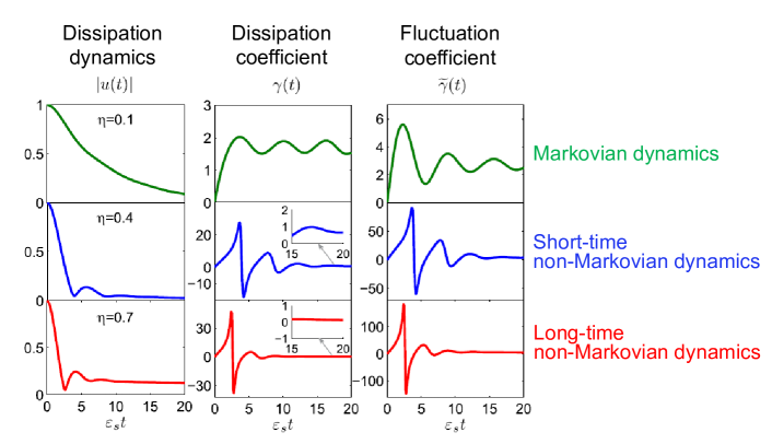
Figure 1: The non-Markovian dynamics in a bosonic system coupled to a sub-Ohmic reservoir $J(\epsilon)=2\pi\eta\epsilon(\epsilon/\epsilon_{c})^{s-1}e^{-\epsilon/\epsilon_{c}}$ with $s=1/2$ PRL2012 . The energy cut-off $\epsilon_{c}=\varepsilon_{s}$ and the initial reservoir temperature $k_{B}T=\varepsilon_{s}$. Here we have taken $t_{0}=0$ so that we define $u(t,t_{0})=u(t)$, $\gamma(t,t_{0})=\gamma(t)$ and $\widetilde{\gamma}(t,t_{0})=\widetilde{\gamma}(t)$.

We have also introduced a quantitative measure of non-Markovian dynamics in terms of two-time correlation functions in the same framework PRA2015 :

$${\cal N}(t,\tau)= \Bigg{|}\frac{\langle A(t)B(t+\tau)\rangle}{\sqrt{\langle A(t)B(t)\rangle\langle A(t+\tau)B(t+\tau)\rangle}}$$

$$-\frac{\langle A(t)B(t+\tau)\rangle_{\textrm{B}M}}{\sqrt{\langle A(t)B(t)\rangle_{\textrm{B}M}\langle A(t+\tau)B(t+\tau)\rangle_{\textrm{B}M}}}\Bigg{|},$$ (27)

where $A$ and $B$ are two physical observables of the system. The exact two-time correlation function $\langle A(t)B(t+\tau)\rangle$ can be obtained either from experiment or theoretical calculations, and the two-time correlation function $\langle A(t)B(t+\tau)\rangle_{\textrm{B}M}$ can be evaluated through the BM master equation. For example, exact two-time current-current correlation $\langle I(t)I(t+\tau)\rangle$ in nano-electronic systems has been theoretically calculated Yang2014 and has recently been measured experimentally CurrentCurrent . The two-time particle number correlation $\langle n(t)n(t+\tau)\rangle$ for photonic systems is also experimentally measured through photon bunching and antibunching experiments antibunching1 ; antibunching2 , and the exact theoretical calculation is carried out in our recent work Ali2017 . More two-time intensity correlation functions have been experimentally measured in optical measurements malik ; Livet ; sutton . While, the calculation of two-time correlation function $\langle A(t)B(t+\tau)\rangle_{\textrm{B}M}$ is rather simple under Born-Markovian approximation. Detailed discussions can be found from PRA2015 . Thus, a quantitative measure of non-Markovian dynamics can be given through two-time correlation functions which provide the direct physical picture of memory dynamics in open quantum systems.

As an illustration, in Fig. 2, we present the non-Markovian dynamics measure through the two-time correlations of the first-order photon coherence function, $\langle a^{\dagger}(t)a(t+\tau)\rangle$, as it precisely characterizes the long-time memory processes arisen from localized bound states ($\eta>\eta_{c}$) and the short-time memory processes resulted from nonexponential decays ($\eta<\eta_{c}$). The memoryless processes in the very weak system-environment coupling regime emerged naturally, and the exact master equation is then reduced to corresponding Born-Markov master equation Xiong2010 . The above general non-Markovian dynamical properties of open quantum systems have also been applied to investigate photonic dynamics in photonic crystals Lei2011 ; Sci2015b , nonequilibrium photon statistics Ali2017 , nonequilibrium quantum phase transition Lin2016 , complexity of quantum-to-classical transition Sci2015a ; decoherence dynamics of Majorana fermion in topological systems PRB18 , and quantum thermodynamics in zero-dimensional systems very recently Ali2018 . On the other hand, the exact master equation theory has also been applied to study various transient quantum transport physics in nanostructures NJP2010 ; ANNP2012 ; PRB2015 ; Yang2014 ; Tu2012 ; Tu2014 ; Liu2016 ; Yang2017 ; Yang2018

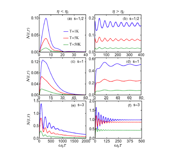
Figure 2: The measure of non-Markovian dynamics in terms of two-time correlation function PRA2015 for a bosonic system coupled to a thermal reservoir with Ohmic-type spectral density $J(\epsilon)=2\pi\eta\epsilon(\epsilon/\epsilon_{c})^{s-1}e^{-\epsilon/\epsilon_{c}}$. The energy cut-off $\epsilon_{c}=5\varepsilon_{s}$ and the system is initially in Fock state with $n=1$, and $t=0$. As it is shown that when the system-reservoir coupling $\eta<\eta_{c}$, no localized bound state exists. Correspondingly, the transient two-time correlation function shows quantitatively that memory effect vanishes when the system approaches to the thermal equilibrium state; while in the strong coupling regime $\eta>\eta_{c}$, the existence of the localized bound state prohibits the system to approach to the equilibrium state, and the non-Markovian dynamics (memory effect) can remains forever.

V Conclusions

In conclusion, we have developed the exact master equation for a large class of non-interacting open quantum systems PRL2012 , including boson systems ANNP2012 and fermion systems PRB2008 ; NJP2010 as well as topological systems PRB18 . The extension to spin systems is also in progress Yao2018 . We established the explicit connection of dissipation and fluctuation dynamics, described by the dissipation and fluctuation coefficients in the exact master equation, with nonequilibrium dynamics in terms of nonequilibrium Green functions. This connection is crucially important because one can then apply the following conclusion to study non-Markovian dynamics of arbitrary interacting open systems, as long as the nonequilibrium Green functions are computable. The conclusion on general non-Markovian dynamics is summarized as follows PRL2012 : the general non-Markovian dynamics is embedded in the time convolution integro-differential equation of the nonequilbrium Green functions. In particular, the dissipation dynamics is fully determined by the propagating Green function. The general solution of the propagating Green function consists of nonexponential decays and dissipationless oscillations (localized bound states in open quantum systems) PRL2012 , which is indeed a universal property of the propagating Green functions in arbitrary interacting many-body systems, according to the general principle of quantum field theory Peskin1995 . The non-exponential decays described by time-dependent decay rates oscillate between positive (dissipation) and negative (back flowing) values in a short time, resulting in the short-time non-Markovian dynamics PRA2015 ; Caldeira1983 . The localized bound states give dissipationless oscillations that make the states of open systems depend forever to its initial state, as a long-time non-Markovian dynamics. Correspondingly, the open system is unable to approach to the thermal equilibrium state of the environment, a property that initially noticed by Anderson long time ago Anderson1961 and is recently justified by us in our exact master equation theory Sci2015a ; Sci2015b . The fluctuating correlation (Keldysh) Green function, determined by the generalized nonequilibrium fluctuation-dissipation theorem [see Eq. (22)], has the similar behaviors as the dissipation dynamics, namely it contains both the short-time and long-time non-Markovian memory effects associated respectively with the continuous spectrum part and the localized bound state part of open systems. This general picture of non-Markovian memory dynamics is fully determined by the energy structures of the system and the environment, and the couplings between them, including also the initial states of the system and the environment, and is irrelevant to any mathematical definition of non-Markovianity.

References

- (1) K. Huang, Statistical Mechanics, 2nd Edition (John Wiley & Sons, New York, 1987) p.189-191.
- (2) W. Pauli, Festschrift zum 60. Geburtstage A. Sommerfelds (Hirzel, Leipzig, 1928) p.30.
- (3) L. van Hove, Quantum-mechanical perturbations giving rise to a statistical transport equation. Physica, 21 (1954) 517.
- (4) S. Nakajima, On quantum theory of transport phenomena: steady diffusion. Prog. Theo. Phys. 20 (1958) 948.
- (5) R. Zwanzig, Ensemble method in the theory of irreversibility. J. Chem. Phys. 33 (1960) 1338.
- (6) F. Haake, Z. Phys. On a Non-Markoffian master-equation: derivation and general discussion. 223 (1969) 353; 364.
- (7) V. Gorini, A. Kossakowski, E.C.G. Sudarshan, Completely positive dynamical semigroups of N-level systems. J. Math. Phys. 17 (1976) 821.
- (8) G. Lindblad, On the generators of quantum dynamical semigroups. Comm. Math. Phys. 48 (1976) 119.
- (9) A. O. Caldeira and A. J. Leggett, Path integral approach to quantum Brownian motion. Physica 121A (1983) 587.
- (10) R. P. Feynman and F. L. Vernon, The theory of a general quantum system interacting with a linear dissipative system, Ann. Phys. (N.Y.) 24 (1963) 118.
- (11) U. Weiss, Quantum Dissipative Systems, 3rd Ed. (World Scientific, Singapore, 2008).
- (12) W. M. Zhang, P. Y. Lo, H. N. Xiong, M. W. Y. Tu, and F. Nori, General non-Markovian dynamics of open quantum systems, Phys. Rev. Lett. 109 (2012) 170402.
- (13) M. W. W. Tu, W. M. Zhang, Non-Markovian decoherence theory for a double-dot charge qubit, Phys. Rev. B 78 (2008) 235311.
- (14) J. Jin, M. W. U. Tu, W. M. Zhang, and Y. J. Yan, Non-equilibrium quantum theory for nanodevices based on the Feynman-Vernon influence functional, New J. Phys. 12 (2010) 083013.
- (15) C. U Lei and W. M. Zhang, A quantum photonic dissipative transport theory, Ann. Phys. 327 (2012) 1408.
- (16) P. Y. Yang, C. Y. Lin, and W. M. Zhang, Master equation approach to transient quantum transport in nanostructures incorporating initial correlations, Phys. Rev. B 92 (2015) 165403.
- (17) H. L. Lai, P. Y. Yang, Y. W. Huang, and W. M. Zhang, Exact master equation and non-Markovian decoherence dynamics of Majorana zero modes under gate-induced charge fluctuations, Phys. Rev. B 97 (2018) 054508.
- (18) P. W. Anderson, Absence of diffusion in certain random lattices, Phys. Rev. 109 (1958) 1492; Localized magnetic states in metals, Phys. Rev. 124 (1961) 41.
- (19) U. Fano, Effects of configuration interaction on intensities and phase shift, Phys. Rev. 124 (1961) 1866.
- (20) C. Cohen-Tannoudji, J. Dupont and G. Grynberg, Atom-Photon Interactions (Wiley, New York, 1992).
- (21) P. Lambropoulos, G. M. Nikolopoulos, T. R. Nielsen, and S. Bay, Fundamental quantum optics in structured reservoirs. Rep. Prog. Phys. 63 (2000) 455.
- (22) G. D. Mahan, Many-Body Physics, 3rd Ed. (Kluwer Academic/Plenum Publishers, New Yoek, 2000), p.207-208.
- (23) J. Schwinger, Brownian motion of a quantum oscillator, J. Math. Phys. 2 (1961) 407.
- (24) L. V. Keldysh, Diagram technique for nonequilibrium processes, Sov. Phys. JETP 20 (1965) 1018.
- (25) L. P. Kadanoff, and G. Baym, Quantum Statistical Mechanics (Benjamin, New York, 1962).
- (26) H. N. Xiong, W. M. Zhang, X. Wang, and M. H. Wu, Exact non-Markovian cavity dynamics strongly coupled to a reservoir, Phys. Rev. A 82 (2010) 012105.
- (27) P. Y. Lo, H. N. Xiong and W. M. Zhang, Breakdown of Bose-Einstein distribution in photonic caystals, Sci. Rep. 5 (2015) 9423.
- (28) H. N. Xiong, P. Y. Lo, W. M. Zhang, D. H. Feng and F. Nori, Non-Markovian complexity in quantum-to-classical transition, Sci. Rep. 5 (2015) 13353.
- (29) M. M. Ali, P. Y. Lo, M. W. Y. Tu, and W. M. Zhang, Non-Markovianity measure using two-time correlation functions, Phys. Rev. A 92 (2015) 062306.
- (30) C. U Lei and W. M. Zhang, Decoherence suppression of open quantum systems through a strong coupling to non-Markovian reservoirs, Phys. Rev. A 84 (2011) 052116.
- (31) M. M. Ali and W. M. Zhang, Nonequilibrium transient dynamics of photon statistics, Phys. Rev. A 95 (2017) 033830.
- (32) I. de Vega and D. Alonso, Dynamics of non-Markovian open quantum systems, Rev. Mod. Phys. 89 (2017) 015001.
- (33) M. M. Wolf, J. Eisert, T. S. Cubitt, and J. I. Cirac Assessing non-Markovian quantum dynamics, Phys. Rev. Lett. 101 (2008) 150402.
- (34) Á. Rivas, S. F. Huelga, and M. B. Plenio, Entanglement and non-Markovianity of quantum evolutions, Phys. Rev. Lett. 105 (2010) 050403.
- (35) H. P. Breuer, E. M. Laine, and J. Piilo, Measure for the degree of non-Markovian behavior of quantum processes in open systems. Phys. Rev. Lett. 103 (2009) 210401.
- (36) R. P. Feynman and A. R. Hibbs, Quantum Mechanics and Path Integrals, (McGraw-Hill, New York, 1965).
- (37) H. Haug and A.-P. Jauho, Quantum kinetics in transport and optics of semiconductors, 2nd Ed. (Springer Series in Solid-State Sciences 123, Berlin, 2007).
- (38) Y. Imry, Introduction to Mesoscopic Physics, 2nd ed. (Oxford University Press, Oxford, 2002).
- (39) K. O. Friedrichs, On the perturnation of continuous spectra, Commun. Pure Appl. Math. 1 (1948) 361.
- (40) T. D. Lee, Some special examples in renormalizable field theory, Phys. Rev. 95 (1954) 1329.
- (41) I. Prigogine, Dissipative processes in quantum theory, Phys. Rep. 219 (1992) 93.
- (42) P. L. Knight, M.A. Lauder, B.J. Dalton, Laser-induced continuum structures, Phys. Rep. 190 (1990) 1.
- (43) H. J. Carmichael, An Open systems approach to quantum optics, lecture notes in physics, Vol. m18 (Springer-Verlag, Berlin, 1993).
- (44) W. M. Zhang and L. Wilets, Transport theory of relativistic heavy-ion collisions with chiral symmetry, Phys. Rev. C 45 (1992) 1900.
- (45) M. E. Peskin and D. V. Schroeder, An Introduction to Quantum Field Theory (Addison-Wesley, Reading, 1995).
- (46) F. Haake and R. Reibold, Strong damping and low-temperature anomalies for the harmonic oscillator. Phys. Rev. A 32 (1985) 2462
- (47) B. L. Hu, J. P. Paz, Y. H. Zhang, Quantum Brownian motion in a general environment: Exact master equation with nonlocal dissipation and colored noise, Phys. Rev. D 45 (1992) 2843
- (48) H. Grabert, P. Schramm, and G.-L. Ingold, Quantum Brownian motion: The functional integral approach, Phys. Rep. 168 (1988) 115.
- (49) R. Karrlein and H. Grabert, Exact time evolution and master equations for the damped harmonic oscillator, Phys. Rev. E 55 (1997) 153.
- (50) A. J. Leggett, S. Chakravarty, A. T. Dorsey, M. P. A. Fisher, A. Garg, and W. Zwerger, Dynamics of the dissipative two-state system, Rev. Mod. Phys. 59 (1987) 1.
- (51) These processes are unreliable because they violate the fundamental principle of energy conservation for each physics process in quantum theory Peskin1995 . These processes could occur in interacting quantum systems as a high-order contribution, but it cannot appear in the bare Hamiltonian in the quantum regime.
- (52) E. T. Jaynes and F.W. Cummings, Comparison of quantum and semiclassical radiation theories with application to the beam maser, Proc. IEEE. 51 (1963) 89.
- (53) C. Anastopoulos and B. L. Hu, Two-level atom-field interaction: Exact master equations for non-Markovian dynamics, decoherence, and relaxation, Phys. Rev. A 62 (2000) 033821.
- (54) H. Z. Shen, M. Qin, X.-M. Xiu, and X. X. Yi, Exact non-Markovian master equation for a driven damped two-level system, Phys. Rev. A 89 (2014) 062113.
- (55) S. J. Whalen and H. J. Carmichael, Time-local Heisenberg-Langevin equations and the driven qubit, Phys. Rev. A 93 (2016) 063820.
- (56) L. D. Faddeev and A. A. Slavnov, Gauge Fields: Introduction to Quantum Theory, (Benjamin-Cummings, Reading, MA, 1980)
- (57) R. Gilmore, Lie Groups, Lie Algebras and Some of Their Applications, (John Wiley & Sons, New York, 1974).
- (58) W. M. Zhang, D. H. Feng, and R. Gilmore, Coherent States: Theory and Their Applications, Rev. Mod. Phys. 62 (1990) 867.
- (59) B. M. Garraway, Nonperturbative decay of an atomic system in a cavity, Phys. Rev. A 55 (1997) 2290.
- (60) H.-P. Breuer, B, Kappler, and F. Petruccione, Stochastic wave-function method for non-Markovian quantum master equations, Phys. Rev. A 59 (1999) 1633.
- (61) R. Doll, D. Zueco, M. Wubs, S. Kohler, P. Hänggi, On the conundrum of deriving exact solutions from approximate master equations, Chem. Phys. 347 (2008) 243.
- (62) H.-S. Goan, C.-C. Jian, and P.-W. Chen, Non-Markovian finite-temperature two-time correlation functions of system operators of a pure-dephasing model, Phys. Rev. A 82 (2010) 012111.
- (63) M. J. Schmidt,D. Rainis, and D. Loss, Decoherence ofMajorana qubits by noisy gates, Phys. Rev. B 86 (2012) 085414.
- (64) H.-P. Breuer and F. Petruccione, The Theory of Open Quantum System (Oxford: Oxford University Press, 2002).
- (65) J. Jin, X. Zheng and Y. J. Yan, Exact dynamics of dissipative electronic systems and quantum transport: Hierarchical equations of motion approach, J. Chem. Phys. 128 (2008) 234703.
- (66) M. Thorwart, M. Grifoni and P. Hänggi, Strong Coupling Theory for Tunneling and Vibrational Relaxation in Driven Bistable Systems, Ann. of Phys. 293 (2001) 15.
- (67) H. T. Tan, and W. M. Zhang, Non-Markovian dynamics of an open quantum system with initial system-reservoir correlations: A nanocavity coupled to a coupled-resonator optical waveguide, Phys. Rev. A 83 (2011) 032102.
- (68) P. Y. Yang and W. M. Zhang, Exact homogeneous master equation for open quantum systems incorporating initial correlations, arXiv:1605.08521 (2016).
- (69) P. Nalbach and M. Thorwart, Ultraslow quantum dynamics in a sub-Ohmic heat bath, Phys. Rev. B 81 (2010) 054308.
- (70) P. Y. Yang, C. Y. Lin and W. M. Zhang, Transient current-current correlations and noise spectra, Phys. Rev. B 89 (2014) 115411.
- (71) K. Thibault, J. Gabelli, C. Lupien, and B. Reulet, Pauli-Heisenberg Oscillations in Electron Quantum Transport, Phys. Rev. Lett. 114 (2015) 236604.
- (72) R. H. Brown and R. Q. Twiss, Correlation between Photons in two Coherent Beams of Light, Nature 177 (1956) 27.
- (73) H. J. Kimble, M. Dagenais, and L. Mandel, Photon Antibunching in Resonance Fluorescence, Phys. Rev. Lett. 39 (1977) 691.
- (74) A. Malik, A. R. Sandy, L. B. Lurio, G. B. Stephenson, S. G. J. Mochrie, I. McNulty, Coherent X-Ray Study of Fluctuations during Domain Coarsening, and M. Sutton, Phys. Rev. Lett. 81 (1998) 5832.
- (75) F. Livet, F. Bley, R. Caudron, E. Geissler, D. Abernathy, C. Detlefs, G. Grubel, and M. Sutton, Kinetic evolution of unmixing in an AlLi alloy using x-ray intensity fluctuation spectroscopy, Phys. Rev. E 63 (2001) 036108.
- (76) M. Sutton, K. Laaziri, F. Livet, and F. Bley, Using coherence to measure two-time correlation functions, Opt. Express 11 (2003) 2268.
- (77) Y. C. Lin, P. Y. Yang and W. M. Zhang, Nonequilibrium quantum phase transition via entanglement decoherence dynamics, Sci. Rep. 6 (2016) 34804.
- (78) M. M. Ali and W. M. Zhang, Quantum Thermodynamics in single particle systems, arXiv:1803.04658 (2018).
- (79) M. W. Y. Tu, W. M. Zhang, J. S. Jin, O. Entin-Wohlman and A. Aharony, Transient quantum transport in double-dot Aharonov-Bohm interferometers, Phys. Rev. B 86 (2012) 115453.
- (80) M. W. Y. Tu, A. Aharony, W. M. Zhang, and O. Entin-Wohlman, Real-time dynamics of spin-dependent transport through a double-quantum-dot Aharonov-Bohm interferometer with spin-orbit interaction, Phys. Rev. B 90 (2014) 165422.
- (81) J. H. Liu, M. W. Y. Tu and W. M. Zhang, Quantum coherence of the molecular states and their corresponding currents in nanoscale Aharonov-Bohm interferometers, Phys. Rev. B 94 (2016) 045403.
- (82) P. Y. Yang and W. M. Zhang, Master equation approach to transient quantum transport in nanostructures, Frontiers of Physics, 12 (2017) 127204.
- (83) P. Y. Yang and W. M. Zhang, Buildup of Fano resonance in the time domain in doubale-dot Aharonov-Bohm interferometer, Phys. Rev. B 97 (2018) 045301.
- (84) J. C. Yao and W. M. Zhang, in progress.