Statistics of Vector Manakov Rogue Waves

Abstract

We present a statistical analysis based on the height and return time probabilities of high amplitude wave events in both focusing and defocusing Manakov systems. We find that analytical rational/semirational solutions, associated with extreme, rogue wave (RW) structures, are the leading high amplitude events in this system. We define the thresholds for classifying an extreme wave event as a RW. Our results indicate that there is a strong relation between the type of the RW and the mechanism which is responsible for its creation. Initially, high amplitude events originate from modulation instability. Upon subsequent evolution, the interaction among these events prevails as the mechanism for RW creation. We suggest a new strategy for confirming the basic properties of different extreme events. This involves the definition of proper statistical measures at each stage of the RW dynamics. Our results point to the need for defining new criteria for identifying RW events.

I Introduction

The emergence, dynamics and prediction of rogue waves (RW), also referred to as freak waves or extreme events, has been in the focus of interest in diverse fields of science (oceanography, physics of fluids, optics, matter waves physics, sociology, bio-sciences,…) over the last fifteen years 1 ; 2 ; 3 ; 3a . However, there are still more open questions than answers concerning the definition, genesis, dynamics, predictability and controllability of RW phenomena 4 ; 5 . This RW debate has stimulated the comparison of predictions and observations among distinct topical areas, in particular between optics and hydrodynamics rep ; a2 .

Peregrine solitons c1 and Akhmediev breathers c2 are well-known RW candidates: they represent solutions of the scalar one-dimensional self-focusing nonlinear Schrodinger equation (NLSE); the Peregrine solitons with the property of being localized in both the transverse and evolution coordinates, the Akhmediev breathers being periodic in the transverse coordinate and localized in the evolution dimension. The Peregrine type solitons are unique also in a mathematical sense, since they are written in terms of rational functions of coordinates, in contrast to most of the other known solutions of the NLSE, which are purely exponential. Recent experiments have provided a path for generating Peregrine solitons in optical fibers with standard telecommunication equipment 4 , as well as in water-wave tanks 5a ; 5b . To the contrary, in the scalar case the defocusing nonlinear regime does not allow for RW solutions, even of a dark nature.

Recently, progress has been made by extending the search for RW solutions to coupled-wave systems. Indeed, numerous physical phenomena require to model waves with two, or more components, in order to account for different modes, frequencies, or polarizations. In those cases, the focusing regime is not a prerequisite for the existence of RW solutions. When compared with scalar dynamical systems, vector systems may allow for energy transfer between the coupled waves, which may yield new families of vector RW solutions (bright-bright, bright-dark type), with relatively complex dynamics. Such types of RWs have recently been found as solutions of, e.g., the focusing vector NLSE 5 ; 6 ; 7 ; 8 , the three-wave resonant interaction equations 9 ; 10 , the coupled Hirota equations 11 , and the long-wave-short-wave resonance 12 . It is crucial to add that new RW families can be created in the defocusing nonlinear regime too. This was shown theoretically and experimentally in 6 ; 13 ; b1 ; b2 ; b3 : its authors proved that, in the defocusing regime of the Manakov system, the range of existence of rational solutions of different types (bright-dark, dark-dark), which are the most serious candidates for RW, overlaps with the region of baseband modulation instability (MI). Moreover, it was demonstrated that MI is a necessary but not sufficient condition for the existence of RWs. It is generally recognized that MI is one of the mechanisms for the RW generation, and recent observations of higher-order MI on the water surface have been reported 5c .

However, a basic question arises regarding the statistical description of high amplitude events in the course of nonlinear wave propagation. It should be considered that under realistic circumstances the propagation medium exhibits fluctuations of its parameters, hence of the background continuous wave (CW) solutions. To describe both bright and dark structures on a background, the term high amplitude wave is used in the sense that it denotes either high amplitude peaks or dips on a background. In addition, it is important to develop a global understanding of RW emergence in a turbulent environment, which connects with the broad topic of wave turbulence in integrable systems 14 . In this respect, we may distinguish two ways of seeding MIs. The first mechanism is associated with noise-driven MI. It refers to the amplification of initial noise superposed on a plane wave solution, which leads to spontaneous pattern formation from stochastic input wave fluctuations. The second mechanism is that of coherently driven MI, which refers to the preferential amplification of a specific perturbation (thus leading to a particular breather solution) with respect to broadband noise. It was shown that breather wave dynamics is subject to competitive interactions of the two types of seeding of MIs 14 . Nevertheless, a complete physical picture of these various phenomena is still lacking.

Moreover, outside the context of discrete systems and numerical studies of supercontinuum generation new1 , the statistical analysis has not yet found a leading role in the studies of RWs, although RWs are statistically determined entities. In our research, we shall provide a new insight into the origin and dynamics of multiparametric vector RW solutions, by adopting a statistical approach. A similar study has been very recently applied to characterize vector RW generation in highly birefringent optical fibers new . In that case, a key role in the RW generation mechanism is played by the presence of group velocity walk-off between the two polarization components, and third order dispersion.

In this paper we statistically investigate the behavior of high amplitude events in the integrable Manakov system. For this end, we numerically model the (light/matter) wave propagation in the nonlinear media (photonic/Bose-Einstein condensate), in the simplest case of a two component system. Physically this corresponds to the case of two orthogonal polarization states of light, or two different atomic states in BEC bec16 . The initial conditions of the wave system represent a crucial issue in our study. In order to simulate fluctuations in the properties of a real system, we shall consider the injection of plane waves with additive white noise in the system. The long time numerical simulations will be performed by means of the pseudo-spectral Fourier method, in order to obtain a proper statistical ensemble of high amplitude events. Note that the term time will be used as a synonym of the propagation length in the following. A brief description of applied numerical and statistical methods is presented in Section 2. The results and their interpretation with respect to different types of RW candidates, different mechanisms of high amplitude events creation and their statistical and dynamical properties are considered in details in Section 3. All results lead us to conclude that new criteria for identifying high amplitude events are necessary. Conclusions and comments are given in Section 4.

II The model equations

The vector nonlinear Schrödinger equations, i.e., the Manakov system, can be written in dimensionless form as

$$i\frac{\partial u^{(1)}}{\partial z}+\frac{\partial^{2}u^{(1)}}{\partial t^{2}}-2s(|u^{(1)}|^{2}+|u^{(2)}|^{2})u^{(1)} = 0$$

$$i\frac{\partial u^{(2)}}{\partial z}+\frac{\partial^{2}u^{(2)}}{\partial t^{2}}-2s(|u^{(1)}|^{2}+|u^{(2)}|^{2})u^{(2)} = 0,$$ (1)

where $u^{(1)}(t,z)$ and $u^{(2)}(t,z)$ represent the wave envelopes, $z$ is the evolution variable, and $t$ is a second independent variable. The meaning of variables depends on the particular applicative context (fluid dynamics, plasma physics, BEC, nonlinear optics, finance). The parameter $s=-1$ refers to the focusing (or anomalous dispersion) regime, while $s=1$ refers to the defocusing (or normal dispersion) regime of wave propagation in the nonlinear medium. Model equation (1) is fully integrable, and it can be solved by applying the Darboux dressing technique 6 ; 13 . Being focused on high amplitude events, we mention briefly the rational or semirational localized solutions of Eq. (1), which are considered as one of the most promising candidates for RW events in the literature 6 ; 13 .

In the focussing case, such rational solutions can be expressed in the form of different bright-dark breather composites 6 : e.g., a boomeron-type soliton with a time-dependent velocity, a breather-like wave resulting from the interference between the dark and bright contributions, and more complex structures resulting from the merging of Peregrine and breather solutions. The last case provides the evidence of an attractive interaction between the dark-bright wave and the Peregrine soliton solutions. In Fig. 1 we present numerically obtained examples of localized wave structures in the focusing case, which are initialized by a plane wave in the form

$$u_{0}^{(j)}=a_{j}e^{i(q_{j}t-\nu_{j}z)},\quad\nu_{j}=q_{j}^{2}+2(a_{1}^{2}+a_{2}^{2}),\quad j=1,2,$$ (2)

with simultaneously added small periodic and random perturbations. The $a_{j}$ parameters represent the initial amplitudes of component waves in the system, while $q_{j}$ are the initial phases. The difference of phase factors $q_{1}-q_{2}=2q$ will be used to present our numerical results in the next sections.

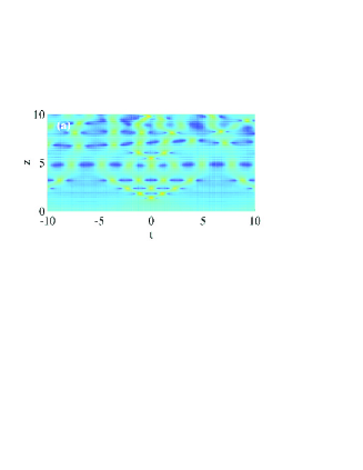
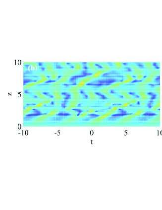
Figure 1: Localized patterns in the focusing Manakov system for $a_{1}(0)=a_{2}(0)=1$ and $q_{1}=q_{2}=0,\,q=0$ ($|u^{(1)}(t,z)|$) (a), $q_{2}=-q_{1}=1,q=1$ (plots of two components $|u^{(1)}(t,z)|$ and $|u^{(2)}(t,z)|$ are shown separately) (b) and (c). The absolute values of the corresponding amplitudes are shown in the box (i. e. the colorbar) in the last plot, and it is mutual for all plots in the figure. Initial small uniform random and periodic perturbations are added to the plane wave background which is amplitude modulated by a super Gaussian.

On the other hand, in the defocusing case the rational/semirational solutions were explicitly derived in 13 . They can be generated both analytically and numerically by starting from a plane wave solution (2). It was analytically shown 13 that the region of rational wave existence, which is related to the domain of RW existence, is determined by the following expression

$$(a_{1}^{2}+a_{2}^{2})^{3}-12(a_{1}^{4}-7a_{1}^{2}a_{2}^{2}+a_{2}^{4})q^{2}+48(a_{1}^{2}+a_{2}^{2})q^{4}-64q^{6}>0.$$ (3)

In particular, the inequality (3) implies that the background amplitudes have to be sufficiently large, for a fixed $q$, in order to allow for the rational wave formation, see Fig. 2. Here, we prefer not to use the term RW for high amplitude rational solutions, since an unique definition of RWs does not exist. Indeed, the findings presented in the following will sustain our terminology. Examples of these rational/semi-rational solutions of the defocusing nonlinear Manakov system are shown in Fig. 2 (a,b). By adding to the finite background small regular (periodic) and random perturbations in the parameter regimes associated with the presence of MI, we confirmed the analytical predictions and previous numerical results from the literature, 13 . The preparation of initial conditions included the presence of a super-Gaussian amplitude modulation of the background. This was done in order to ensure conditions that would isolate the MI mechanism from possible presence of numerical artifacts (e.g., boundary reflections).

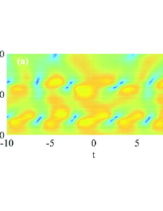
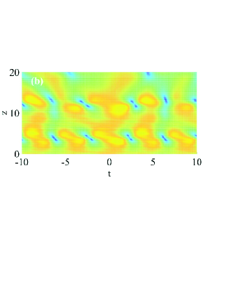
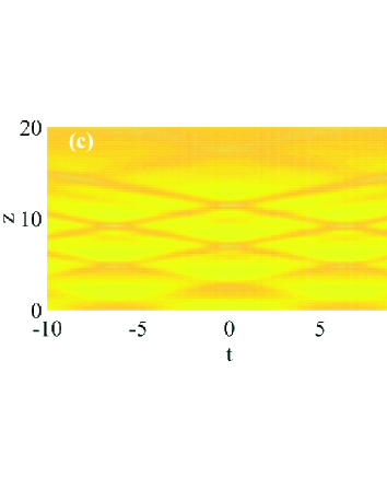
Figure 2: Localized patterns ($|u^{(1)}(t,z)|$ and ($|u^{(2)}(t,z)|$) in the defocusing Manakov system for $a_{1}(0)=a_{2}(0)=0.8$, $q_{2}=-q_{1}=1,\,q=1$ (a,b) (region of existence of rational solitons). In plot (c) the case outside the region of the rational RW existence reported in 13 is presented, with $a_{1}=a_{2}=1,\,q=0$ ($|u^{(1)}(t,z)|$). The absolute values of the corresponding amplitudes are shown in the box (i. e. the colorbar) in the last plot, and it is mutual for all plots in the figure. Initially small cosine and uniform random perturbations are added to the plane wave background, amplitude modulated by a super Gaussian.

The next step was to prepare initial conditions that can ensure the generation of a huge ensemble of localized, high amplitude events, which is necessary for the statistical analysis. We analyzed the results of numerical simulations with different initial conditions, namely, a plane wave (uniform background) with random perturbations (white noise, Gaussian noise), with a small periodic (coherent) perturbation, and with a combination of both small random and periodic perturbations. In all cases, qualitatively the the same behavior was obtained. Therefore, we decided to perform numerical simulations by injecting a noise seeded plane-wave field into the model equations, (1). We applied the standard split-step numerical procedure for solving the evolution equations, 16 . In order to obtain a qualitative confirmation of our numerical findings, we applied, in parallel, the sympletic variants of the split-step method: SABA2 and SBAB2 algorithms sympl . Qualitatively, the same results and conclusions were obtained.

Amplitude noise is numerically modeled as a uniform random process with zero mean. In order to have sufficient data for the statistical analysis, the long term evolution of the field was numerically simulated. The optimal width of the calculation window was estimated in each particular case by repeated numerical tests.

III Statistics of the Manakov rogue waves

The purpose of this study is the statistical analysis of the emergent peaks (dips) in the numerical solutions of the Manakov system. Such extreme amplitude wave events are usually referred to as RWs, whenever the significant height criterion is satisfied 17 ; statistics . Here, the difference between the maximum value of the finite background elevation in between two zero-crossings and the minimum value of the background elevation in the adjacent (next or previous) zero crossing interval is called the wave height (Fig. 3). In scalar models of water-wave propagation, the significant height $h_{s}$ is defined traditionally as the average height of one-third of the highest waves in the height distribution, and the RW threshold is estimated to be $h_{th}\geq 2.2h_{s}$ (also, in the literature on ocean rogue waves, waves with height bigger than $2h_{s}$ qualify to be in this category Kharif .

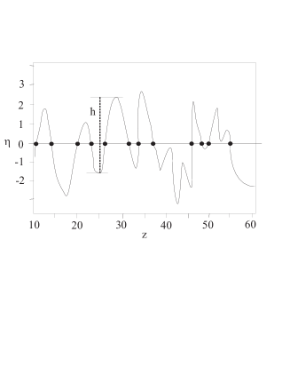
Figure 3: The schematic illustration of determination of the wave height. Quantity $\eta(z)=|u(z)|-|u(0)|$ is the wave amplitude elevation rep .

In the preparatory phase of our study, we searched for proper RW classifiers. Recently, a two-dimensional (2D) equivalent of the significant wave height was defined as a classifier in vector models (18 ). In the framework of the complex RW patterns that are observed in our model, this does not seem as an appropriate criterion to declare that an event is of the RW type. Defining a new, proper classifier(s) remains a challenge for future studies. Here, the significant height criterion is slightly modified: we introduce a vector ($\hat{h}_{s})$, where each of its components measures the significant height of the respective field component $(h^{(j)}_{s},\,j=1,2$)

$$\hat{h}_{s}=(h^{(1)}_{s}\,h^{(2)}_{s})^{T}.$$ (4)

In this expression, the abbreviation $T$ indicates the transpose operation. Thus, the height threshold, ($\hat{h}_{th})$, is a vector quantity consisting of the height thresholds with respect to two spinor components, $(h^{(j)}_{th},\,j=1,2$). Finally, if at least a height of one of the components reaches the corresponding threshold height, the event is declared as a RW. Let us note that the threshold criterion for each particular component is the same as the usual one for the one-dimensional case: $h^{(j)}_{th}=2.2\,h^{(j)}_{s},\,j=1,2$. However, the proper definition of the height criterion for a RW in multi-component system remains still an open issue. For the sake of simplicity, the vector abbreviations for significant height and threshold height will be omitted in the following ($\hat{h}_{s}=h_{s},\hat{h}_{th}=h_{th})$.

We calculated different statistical measures which have been developed in the literature on extreme events, and considered their relevance for expressing the dynamical properties of high amplitude events in the Manakov system. It was shown that the most adequate statistical measure for our system is that based on the height and return time, namely, the probability density of the wave height $P_{h}$, or height probability density (HPD) nash ; new , coupled with the probability distribution of the return time among to successive RW events, i.e., $P_{r}$, 20 .

In the following, we will discuss the shape of the $P_{h}$ curves (associated with the corresponding moments) as a function of $h_{s}$, along with the probability of RW occurrence $P_{ee}$, which can be derived from $P_{h}$. The tails of the HPD are related to the presence of extreme events. The probability of RW occurrence is defined as $P_{ee}=P_{h}(h>h_{th}=2.2h_{s})$ (with respect to both vector components), and it is obtained by integration of the normalized $P_{h}$ from $h=h_{th}$ up to infinity.

For a deeper insight into the time statistics of RWs, the probability distribution of the return time (time is a synonym of propagation length/duration), $P_{r}$ of these (vectorial) events was also calculated. The return time $r$ is defined as the time interval between the appearance at given position of two successive events with amplitudes above a certain predetermined height threshold $h_{r}$. Details on the calculation of the return time probability distribution are given in 20 . Briefly, the return time is registered as the time interval between two successive events with a height (i.e., heights of both field components) above a certain threshold value, which appears at the same given lattice location. We follow this procedure repeatedly up to the end of our simulations, or inside the selected time window, and construct histograms of return times for different system parameters. All return times are scaled by the average return time $R$ in each particular simulation. Therefore, the second set of statistical measures consists of the mean return time $R$, the slope of the return time probability function $P_{r}$, and moments derived from them.

IV Results and discussion

The first step was to generate numerically rational solutions which can be classified as RWs. The existence of these solutions had been related, at least initially, with the development of MI 6 ; 13 , which is by itself threshold determined. Intensive numerical checking has shown that the rational solutions of the types presented in 6 ; 13 , see also Figs. 1 and 2, can be obtained from both coherently or noise driven MI 14 , and represent short-lived or transient wave structures. It should be noted that the exact choice of the initial excitation is crucial for the generation of rational solutions in the defocusing case. In this respect, the structures which were analytically derived in 13 from eigenvalues of the Manakov system, have only been observed in the initial phase of the development of baseband MI development, in the presence of a periodically perturbed plane wave background, additionally modulated by a super Gaussian.

Regardless of the initial perturbations, the long term dynamics of high amplitude events in the Manakov system, observed in the presence of MI, shows similar tendencies. This is the case for both types of nonlinearity, that is either focusing or defocusing. Therefore, statistical ensembles were obtained from long term numerical simulations involving a noise seeded plane-wave field as an input condition for the Manakov system (1). As discussed in the next section, the width of the calculation window was adapted in each case in order to include all relevant regimes of high amplitude events.

IV.1 High amplitude events in the focusing case

The evolution of wave amplitudes for two different initial conditions, corresponding to parameters above the MI threshold is presented in Fig.4. Two different regimes can be distinguished on these plots: an initial, transient phase, and a long-term (long propagation lengths) phase. The transient phase is characterized by the existence of distinct high amplitude localized patterns, which can be associated with localized bright and dark rational structures on a finite background. The latter phase has a highly irregular (turbulent) appearance. These qualitative differences are reflected on the respective statistical measures in that they exhibit a different dependence on the width of the temporal calculation window.

On the basis of numerical simulations, we can distinguish between an initial, transient, and subsequent long-term dynamical regime for the ensemble of the high amplitude events. Inside the transient regime, MI is expected to be the governing mechanism for the creation of localized waves, including the rational solutions. These extreme waves appear and disappear, and interact among themselves and the noisy background upon the propagation. This behavior relatively quickly evolves into a ’turbulent’ like, i.e. irregularly looking, long-term regime. Interestingly, this kind of dynamical behavior starts to prevail sooner or later in time, depending on the specific system parameters, but it is always the final state of the system. In order to exclude the numerical uncertainty as a reason for such system behavior, we repeated our simulations with sympletic variants of the split-step numerical procedure. Qualitatively, the same results and conclusions were always obtained.

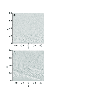
Figure 4: Amplitude evolution plots for the focusing Manakov system with initial plane-wave parameters: (a) $a_{1}=a_{2}=1,\,q=0\,(q_{1}=q_{2}=0)$ and (b) $a_{1}=a_{2}=1,\,q=1\,(q_{2}=-q_{1}=1)$. Both sets of parameters belong to the MI development region. Two regions in these plots can be distinguished with respect to the presence of isolated localized patterns: the region up to $z\approx 30$ and above $z\approx 50$, respectively (indicated by dashed lines). Since the purpose of this figure is to provide a general picture of the dynamics of the system, we only plot the amplitudes of the first component of the vector fields, for the sake of simplicity. Maximum wave amplitude is  $4.5$ (a) and  $4$ (b).

Now concerning the statistical measures, the HPD curves (i.e. $P_{h}$ vs. wave component height) for the sets of parameters corresponding to Fig. 4 are presented in Fig. 5((a) and (b)) in a linear scale, and in Fig. 5 ((c) and (d)) in a log-linear scale. The statistical distributions are obtained for different intervals of the evolution coordinate $z$, as indicated in the legend of Fig. 5. As far as the overall behavior of these curves is concerned, we may observe that the $P_{h}$ curves that characterize the statistics of extreme waves in the initial phase (black squares) differ from those obtained for the irregular phase (red triangles). Also, the $P_{h}$ curves associated with the entire system dynamics (i.e., both initial and irregular phases), which are represented by blue circles, almost coincide with the curves for the long-term phase. One more feature that is evident, is that the maximum of the $P_{h}$ curves shifts towards bigger heights as the calculation window ’moves’ in time. This leads to the conclusion that extreme events occurring in the later, turbulent phase dominate tail distribution associated with RW generation.

In addition, we searched for the best fitting function for the HPDs, following the ideas already presented in the literature new ; new1 . As expected, the observed HPD deviates from a Gaussian probability distribution (this is a known feature of RW statistics). Alternatively, it is possible to model the HPD by means of a generalized Gamma distribution (GGD) new . The GGD is often used in statistics for describing extreme events and it reads as

$$P(x;a,\beta,m)=\frac{a}{\beta\Gamma(m)}\left(\frac{x}{\beta}\right)^{am-1}e^{-(x/\beta)^{a}},$$ (5)

where $a$ and $m$ are shape parameters, and $\beta$ is a scale parameter. In order to account for the normalization of our HPDs, the GGD distribution was multiplied with a parameter $c$, ($0<c<1$). From Fig. 5(c) and Fig. 5(d), it is obvious that the HPDs associated with the long-term (blue circles) and the irregular phase (red triangles) are better fitted with the GGD than the distribution corresponding to the initial phase (black squares), where the discrepancy is most pronounced in the tail sections. Also, it is evident that the agreement is better for the second set of parameters (Fig. 5(d)). However, although the GGD appears to be the function of choice in the interaction region, still it does not reduce to any of the special functions (e.g., Log-normal, Weibull, etc…). The reason for this could be found in the complexity of the processes governing the system behavior. The values of the optimal fitting parameters $a$, $m$ and $\beta$ are listed in Table 1.

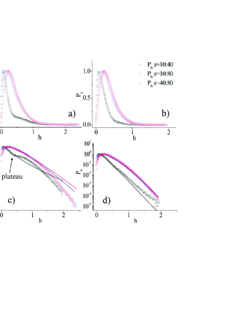
Figure 5: The $P_{h}$ vs. $h$ in linear (upper plots) and semi-logarithmic scales (lower plots) for initial plane-wave parameters: (a,c) $a_{1}=a_{2}=1,\,q=0$ and (b,d) $a_{1}=a_{2}=1,\,q=1\,(q_{2}=-q_{1}=1)$. Different curves correspond to the height distributions of events belonging to different $z$ ranges: black squares $z=10$ to $40$, blue circles $z=10$ to $80$ , red triangles $z=40$ to $80$. In plots (c) and (d), solid lines present GGD fits of the corresponding $P_{h}$ curves.

The corresponding values of the significant height, threshold height and $P_{ee}$ are listed in Table 2. All of these quantities were derived from the $P_{h}$ distribution. The values of $h_{s}$ and $h_{th}$ are of the same order in both selected parameter cases and calculation windows. The values of $P_{ee}$ in the transient and long-term regimes are similar and very small, of the order of $0.001$, i.e. $0.1\%$. Depending on the values of the parameters (amplitudes and phases of initial plane-wave excitation), and therefore on the the position of the MI borderline, the value of $P_{ee}$ has a slight tendency to increase in the transient regime up to $1\%$. The ’plateau’ (indicated by arrow in Fig. 5) in the shape of the corresponding $P_{h}$ curves at medium heights, which are observed in certain parameter areas close to the mentioned border, could be associated with a zero, or small value of the initial phase difference between the wave components of the plane wave $q$, see Fig. 5.

On the other hand, in the presence of nonzero $q$, the transversely moving localized transient modes can be excited via the MI mechanism. In addition, for small heights, the growth rate of $P_{h}$ with $h$ is larger for simulations involving the long-term evolution, when compared with the corresponding growth rate in the early regions where the localized amplitude patterns are clearly visible. In general, this leads to smaller values of $P_{h}$ in the early regime of evolution. Qualitative differences of the $P_{h}$ curves corresponding to different calculation windows undoubtedly show that different types of high amplitude events govern the system behavior in the course of the vector wave propagation. On the other hand, the observed negligible quantitative differences in the $P_{ee}$ indicate the necessity to search for suitable quantifiers of the types of RWs and their dynamics. Once again, this opens the question whether the criterion for RWs based on the significant height is a necessary and a sufficient one.

An additional set of statistical measures for the RWs was derived from the statistics of the return time probability, $P_{r}$, as shown in Fig. 6. The $P_{r}$ curves for two different initial conditions and with respect to (two) different thresholds, $h_{r}$, are comparatively presented in this figure. The shape of the $P_{r}$ curves changes with the position of the calculation window and its width, as well as with the amplitude thresholds. For lower thresholds, the $P_{r}$ curves corresponding to either transient or transient+long term evolution phases exhibit a similar behavior, except for the region corresponding to short return times, see Fig. 6 (a) and (c). The last finding can be associated with the higher influence of the MI mechanism in the transient regime, i.e., the short-lived high amplitude structures are more significant here.

Additionally, for certain initial conditions, one can observe a turning point, i.e., a plateau, in the region of moderate values of the return time. By moving the calculation window from the early transient regime into the long-term limit, the slope of the $P_{r}$ curves changes, and it becomes steeper. However, the tails of all these curves are power-law like. In the long-term regime, a plateau is no longer present on the $P_{r}$ curves. All of this indicates the more frequent appearance of high amplitude events in the transient phase than in the long term situation. The distinction between the $P_{r}$ curves obtained in different evolution windows is lost with respect to highest amplitude events, that are associated here with the condition $h_{r}=2.2h_{s}$, see Fig. 6 (b) and (d). In summary, the MI leads to a transient system behavior, whereas the interactions between moving ’space-time’ localized structures become more significant as the system evolution progresses further. Depending on the system parameters, the length (i.e. the duration) of the transient phase will change. Note that the complexity of the dynamics in transient region, by itself, stems out from the possibility to excite different types of localized rational or exponentially localized solutions.

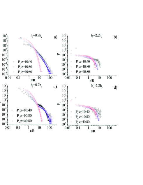
Figure 6: The $P_{r}$ vs. $r/R$ for (a), (b) $a_{1}=a_{2}=1,\,q=0$ and (c), (d) $a_{1}=a_{2}=1,\,q=1\,(q_{2}=-q_{1}=1)$, with respect to different threshold amplitudes $h_{r}$. Three curves in plots (a) and (c) are obtained for $h_{r}=0.7h_{s}$ and those in (b) and (d) for $h_{r}=2.2h_{s}$. Different curves correspond to different calculation windows, as in the previous figure 5. The amplitude threshold values are summarized in Table II due for completeness.

IV.2 High amplitude events in the defocusing case

The same approach of the previous subsection can also be applied to study RW statistics in the defocusing Manakov system. The particularity of this case is the strict dependence of the wave dynamics on the initial conditions, as already mentioned in Section II. The preparation of initial conditions in our numerical experiments differs from that presented in 13 , where the presence of baseband MI was declared as a sufficient condition for the creation of rational/semi-rational solutions. In order to extract any hidden correlation within our findings, we present the results for two set of parameters: $a_{1}=a_{2}=1,q=0$ and $a_{1}=a_{2}=0.8,q_{2}=-q_{1}=1,q=1$, which are outside and inside the baseband MI region, according to Eq. (3), respectively. It should be noted that the properties and values of statistical measures can strongly depend on the system parameters, which are directly related to the position of the border of baseband MI, and the value of its growth rate.

The amplitude plots for both representative parameter sets are presented in Fig. 7. A clear distinction between two evolution phases, which was apparent in the focusing case, is absent in the defocusing regime. However, as we shall see below, the statistical study still shows that, in general, a competition exists among two different mechanisms for creating the high amplitude events. Namely, the competition between baseband MI and wave interactions, as well as the prevalence of the second mechanism in the long-term evolution.

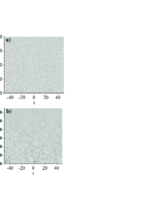
Figure 7: Amplitude evolution plots in the defocusing Manakov system with initial plane-wave parameters: (a) $a_{1}=a_{2}=1,\,q=0$ and (b) $a_{1}=a_{2}=0.8,\,q=1\,(q_{2}=-q_{1}=1)$. First set of parameters is outside the baseband MI region, while the second is inside of it. Maximum amplitude is  4 (a) and  3 (b).

In Fig. 8 we present the wave height probability $P_{h}$ curves together with their GGD fits, for a set of parameters that are either outside (i.e., $a_{1}=a_{2}=1,\,q=0$, see Fig. 7(a) and (c))) or inside (i.e., $a_{1}=a_{2}=0.8,\,q=1$, see Fig. 7(b) and (d)) the range of existence of baseband MI, respectively. We may note here the same qualitative behavior for the shape of $P_{h}$ as previously observed in the focusing case. Once again, the peak of the $P_{h}$ curves shifts towards larger heights as the computation window progresses to include longer term evolutions. The large ’dip’ on the $P_{h}$ curves in the region of medium $h$ for $q=0$, i.e., outside of the baseband MI range, is lost in the long-term calculation windows. A similar ’dip’ was previously observed in the focusing case, where it was associated with the absence of an initial transverse kick, or phase difference between the components of the weak initial wave perturbation. In the defocusing case, this feature can also be related with the absence of baseband MI 13 .

On the other hand, Fig. 8 shows that the $P_{h}$ behavior for calculation windows in the long-term range is statistically the same in both selected parameter cases, namely, either outside or inside the region for baseband MI. Therefore, based on our results, one cannot claim that rational solutions, which have been reported to be a main candidate for RWs in the region of baseband MI, provide the only source of statistically significant high amplitude events in the case $a_{1}=a_{2}=0.8,\,q=1$ (i.e., inside MI region). In fig. 8 the shapes of $P_{h}$ curves as well as the values of $h_{s}$ (see Table 2) and $P_{ee}$ do not show a notable dependence upon the size and position of the calculation window. In general, the values of $h_{s}$ and $P_{ee}$ follow the same scenario as they did in the focusing case. The $P_{ee}$ values are very small, of the order $0.1\%-1\%$, in all parameter regions which are related with the existence of high amplitude events (rational solitons). Modeling the HPD curves with the GGD gave similar results as in the focusing case (Fig. 7(c) and (d)). The agreement between the GGD and HPD is better for the case of initial parameters inside the baseband MI region, especially in the long-term limit. Moreover, in this region, one can notice that the HPDs have a similar shape for both sets of initial parameters. The values of GGD parameters are given in Table 1.

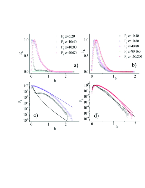
Figure 8: The $P_{h}$ vs. $h$ in linear (upper plots) and semi-logarithmic scales (lower plots) for initial plane-wave parameters: (a,c) $a_{1}=a_{2}=1,\,q=0$ and (b,d) $a_{1}=a_{2}=0.8,\,q=1\,(q_{2}=-q_{1}=1)$. Different curves correspond to the height distributions of events belonging to regions of $z$ are explicitly reported in the plots. On plots (c) and (d), solid lines represent GGD fits of corresponding $P_{h}$ curves.

On the other hand, the return probability $P_{r}$ behavior is illustrated in Fig. 9. For higher values of the threshold amplitude ($h_{r}=2.2h_{s}$), the $P_{r}$ curves show the same tendency with respect to the position of the calculation window for both sets of parameters. By moving the calculation windows towards the long-term region, the slopes of the $P_{r}$ curves for lower threshold ($h_{r}=0.7h_{s}$) increase, whereas the shape of the $P_{r}$ curves does not change with further changes in the position or (width) of the calculation window.

A similar tendency regarding the shape of the $P_{r}$ curves can be recognized for higher threshold values. By comparing the return times of high amplitude events for the two selected thresholds, we can conclude that the return time of the highest amplitude events is smaller than for the rest of the selected events. This is in accordance with the values of $R$ which are presented in Table 2. Note that this is the case for both sets of parameters, i.e., either outside or inside the baseband MI region. On the other hand, the differences in $P_{r}$ and related quantities for calculations windows in the ’transient’ phase are obvious, and can be related to different types of RWs with respect to those in the latter phases of the system evolution. In general, for smaller thresholds, the slopes of the $P_{r}$ curves change in a way similar to that observed in the focusing regime. Namely, the slope of the curve in the long-term (turbulent) regime is steeper than in the transient phase. This correlates with the mechanism responsible for exciting high amplitude events. In the first case, the RW generation is associated with MI, whereas in the second case it is associated with interactions between different high amplitude modes. Note that the $P_{r}$ for both vector field components were calculated, and we confirmed that they obey the same statistical scenario.

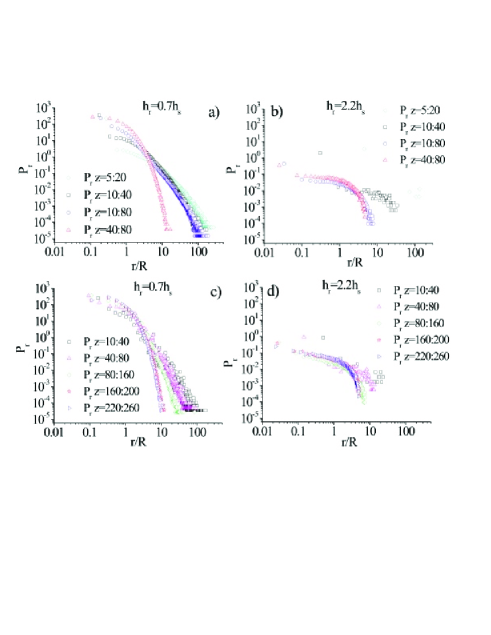
Figure 9: The $P_{r}$ vs. $r/R$ for (a, b) $a_{1}=a_{2}=1,\,q=0$ and (c, d) $a_{1}=a_{2}=0.8,\,q=1\,(q_{2}=-q_{1}=1)$, with respect to different threshold amplitudes $h_{r}$. Three curves in plots (a) and (c) are obtained for $h_{r}=0.7h_{s}$ and those in (b) and (d) for $h_{r}=2.2h_{s}$. Different curves correspond to different calculation windows, as in previous figure 8.

Table 1: GGD fitting parameters for plots in Figs. 5 and 8. The shape parameter values for certain standard distributions are: Gamma distribution, $a=1$, exponential distribution, $a=1,\,m=1$, Rayleigh $a=2,\,m=1$, Weibull distributions $m=1$, and log-normal distribution $m\rightarrow\infty$.

Fig. 4a	$a$	$m$	$\beta$
$z=10:40$	0.430	5.926	0.003
$z=10:80$	1.145	1.381	0.294
$z=40:80$	1.082	2.047	0.211
Fig. 4b	$a$	$m$	$\beta$
$z=10:40$	0.908	2.060	0.088
$z=10:80$	1.264	1.380	0.270
$z=10:40$	1.217	1.799	0.234
Fig. 7a	$a$	$m$	$\beta$
$z=5:20$	1.246	1.148	0.019
$z=10:40$	0.443	5.473	0.002
$z=10:80$	1.163	1.077	0.343
$z=40:80$	0.741	3.234	0.072
Fig. 7b	$a$	$m$	$\beta$
$z=10:40$	0.770	3.420	0.041
$z=10:80$	0.715	3.765	0.037
$z=40:80$	0.735	3.633	0.044
$z=80:160$	1.143	1.924	0.179
$z=160:200$	1.278	1.657	0.229

Table 2: Values of different parameters derived from the $P_{h}$ and $P_{r}$ for focusing and defocusing cases.

$a_{1}=a_{2}=1,\,q=0$
focussing	$z=[10:40]$	$[10:80]$	$[40:80]$
$h_{s}$	$0.549$	$0.673$	$0.697$
$h_{th}$	$1.210$	$1.480$	$1.530$
$P_{ee}$	$0.006$	$0.013$	$9.96e^{-4}$
$R_{1}$	$0.011$	$0.009$	$0.009$
$R_{2}$	$0.026$	$0.021$	$0.019$
$R_{3}$	$2.019$	$8.279$	$8.399$
$a_{1}=a_{2}=1,\,q=1$
focussing	$z=[10:40]$	$[10:80]$	$[40:80]$
$h_{s}$	$0.397$	$0.592$	$0.631$
$h_{th}$	$0.836$	$1.302$	$1.349$
$P_{ee}$	$0.008$	$0.002$	$0.002$
$R_{1}$	$0.015$	$0.011$	$0.009$
$R_{2}$	$0.039$	$0.024$	$0.019$
$R_{3}$	$2.803$	$4.566$	$6.600$

$a_{1}=a_{2}=1,\,q=0$
defoc.	$z=[10:40]$	$[10:80]$	$[40:80]$
$h_{s}$	$0.506$	$0.651$	$0.666$
$h_{th}$	$1.110$	$1.430$	$1.465$
$P_{ee}$	$0.011$	$0.002$	$0.001$
$R_{1}$	$0.011$	$0.010$	$0.009$
$R_{2}$	$0.027$	$0.023$	$0.021$
$R_{3}$	$0.744$	$8.292$	$8.068$

$a_{1}=a_{2}=0.8,\,q=1$
defoc.	$z=[10:40]$	$[10:80]$	$[40:80]$	$[80:160]$	$[160:200]$
$h_{s}$	$0.411$	$0.466$	$0.498$	$0.534$	$0.553$
$h_{th}$	$0.904$	$1.025$	$1.096$	$1.175$	$1.217$
$P_{ee}$	$0.003$	$0.002$	$0.002$	$9.6e^{-4}$	$7.7e^{-4}$
$R_{1}$	$0.011$	$0.011$	$0.011$	$0.009$	$0.009$
$R_{2}$	$0.023$	$0.023$	$0.023$	$0.018$	$0.018$
$R_{3}$	$1.013$	$4.221$	$2.779$	$10.444$	$7.663$

V Conclusions

Let us summarize the results of our study of high amplitude events in the Manakov system, by pointing out the main findings. In both the focusing and defocusing nonlinearity regime, it was shown that the type of initial perturbation of the plane wave background did not have a significant influence on the long term evolution of high amplitude events. On the other hand, we found that the properties of the long term evolution can be associated with the presence of MI in the Manakov system. In latter stages of the evolution of the high amplitude modes, their interactions drive the dynamics of high amplitude events, and potentially affect the properties and the behavior of RWs. This conclusion does not depend on the character of nonlinearity in the Manakov system.

We decided to use the term ’high amplitude events’ instead of ’RWs’, on the basis of the unclear indications about the criteria for extracting RWs from a statistical analysis based on the height and return time probabilities. We have found that the statistics of heights of high amplitude events can be described very well by the generalized Gamma distribution in both the focusing and the defocusing regime, especially in the long term propagation limit, i.e., in a regime where interactions between the high amplitude events are shown to be the most prominent contributors to the RW generation. In contrast, we have shown that, in order to identify a high amplitude event as a RW, new criteria are necessary, at least in multi-component systems. The significant height vector equivalent of the corresponding scalar quantity is not sensitive enough, in order to clearly identify the RW, as well as to distinguish between different types of RWs.

Data derived from the return time probability mostly confirm previous statements, and show that the return time based quantities can be promising candidates for good classifiers of different types of RWs. The significance of the initial system preparation, width and position of the calculation window, on the values of the threshold amplitudes has been pointed out. Therefore, the main contribution of this study is the suggestion and development of a new strategy for confirming the basic properties of different RWs events in multicomponent nonlinear wave systems.

- (1) D. R. Solli, C. Ropers, P. Koonath,and B. Jalali, Nature (London) 450, 1054 (2007).
- (2) Y. V. Bludov, V. V. Konotop, and N. Akhmediev, Phys. Rev. A 80, 033610 (2009).
- (3) Extreme Events in Nature and Society, edited by S. Albevario, V. Jentsch, and H. Kantz (Springer, Berlin, 2006)
- (4) M. Narhi, B. Wetzel, C. Billet, S. Toenger, T. Sylvestre, J-M. Merolla, R. Morandotti, F. Dias, G. Genty, J. M. Dudley, Nature Communications 7:13675 (DOI: 10.1038/ncomms13675) (2016).
- (5) B. Kibler, J. Fatome, C. Finot, G. Millot, F. Dias, G. Genty, N. Akhmediev, and J. M. Dudley, Nature Physics 6, 790 (2010).
- (6) B. L. Guo and L. M. Ling, Chin. Phys. Lett. 28, 110202 (2011).
- (7) M. Onorato, S. Residori, U. Bortolozzo, A. Montina, F.T. Arecchi, Physics Reports 528, 47 (2013).
- (8) M. Onorato, S. Residori, and F. Baronio, Rogue and ShockWaves in Nonlinear Dispersive Media (Springer, Berlin, 2016).
- (9) D. H. Peregrine, J. Austral. Math. Soc. Ser. B 25, 16 (1983).
- (10) N. Akhmediev and A. Ankiewicz, Solitons, Nonlinear Pulses and Beams (Chapman and Hall, London, 1997).
- (11) A. Chabchoub, N. P. Hoffmann and N. Akhmediev, Phys. Rev. Lett. 106, 204502 (2011).
- (12) A. Chabchoub, Phys. Rev. Lett. 117, 144103 (2016).
- (13) F. Baronio, A. Degasperis, M. Conforti, and S. Wabnitz, Phys. Rev. Lett. 109, 044102 (2012).
- (14) L. C. Zhao and J. Liu, Phys. Rev. E 87, 013201 (2013).
- (15) B. G. Zhai, W. G. Zhang, X. L. Wang, and H. Q. Zhang, Nonlinear Anal. Real World Appl. 14, 14 (2013).
- (16) F. Baronio, M. Conforti, A. Degasperis, and S. Lombardo, Phys. Rev. Lett. 111, 114101 (2013).
- (17) A. Degasperis and S. Lombardo Phys. Rev. E 88, 052914 (2013).
- (18) S. Chen and L. Y. Song, Phys. Rev. E 87, 032910 (2013).
- (19) S. Chen, Ph. Grelu, and J. M. Soto-Crespo, Phys. Rev. E 89, 011201(R) (2014).
- (20) F. Baronio, M. Conforti, A. Degasperis, S. Lombardo, M. Onorato, and S. Wabnitz, Phys. Rev. Lett. 113, 034101 (2014); F. Baronio, S. Chen, Ph. Grelu, S. Wabnitz, and M. Conforti, Phys. Rev. A 91, 033804 (2015).
- (21) B. Frisquet, B. Kibler, J. Fatome, P. Morin, F. Baronio, M. Conforti, G. Millot, and S. Wabnitz, Phys. Rev. A 92, 053854 (2015).
- (22) B. Frisquet, B. Kibler, P. Morin, F. Baronio, M. Conforti, G. Millot, and S. Wabnitz, Sci. Rep. 6, 20785 (2016).
- (23) F. Baronio, B. Frisquet, S. Chen, G. Millot, S. Wabnitz, B. Kibler, Phys. Rev. A 97, 013852 (2018).
- (24) O. Kimmoun, H. C. Hsu, B. Kibler, and A. Chabchoub, Phys. Rew. E 96, 022219 (2017).
- (25) E. G. Turitsyna, S. V. Smirnov, S, Sugavanam, N. Tarasov, X. Shu, S. A. Babin, E. V. Podvilov, D. V. Churkin, G. Falkovich, S. K. Turitsyn, Nat. Photonics 7, 783 (2013).
- (26) E. Louvergneaux, V. Odent, M.I. Kobolov, and M. Taki, Phys. Rev. A 87, 063802 (2013).
- (27) L. Drouzi, S. Coulibaly, C. G. L. Tiofack, M. Taki and K. Laabidi, Rogue wave formation in highly birefringent fiber, in: Nonlinear Guided Wave Optics, S. Wabnitz, Ed., Chapter 13 (IOP Publishing, 2017).
- (28) Y. V. Bludov, V. V. Konotop and N. Akhmediev, Eur. Phys. J. Special Topics 85, 033610 (2010).
- (29) G. Gligorić, A. Maluckov, M. Stepić, Lj. Hadžievski, and B. A. Malomed Phys. Rev. A 82, 033624 (2010).
- (30) J. Laskar and P. Robutel, Celest. Mech. Dyn. Astron. 80, 3962 (2001); C. Skokos, D.O. Krimer, S. Komineas, and S. Flach, Phys. Rev. E 79, 056211 (2009).
- (31) C. Kharif and E. Pelinovsky, Eur. J. Mech. B/Fluids. 22, 603 (2003).
- (32) S. Toenger, T. Godin, C. Billet, F. Dias, M. Erkintalo, G. Genty, and J. M. Dudley, Sci. Rep. 5, 10380 (2015).
- (33) C. Kharif et al., Rogue Waves in the Ocean (Springer Berlin Heidelberg) (2009).
- (34) M. J. Ablowitz and T. P. Horikis, J. Opt. 19, 065501 (2017).
- (35) A. Maluckov, N. Lazarides, G. P. Tsironis and Lj. Hadžievski, Phys. Rev. E 79, 025601(R) (2009); A. Maluckov, N. Lazarides, G. P. Tsironis and Lj. Hadžievski, Physica D 252, 59 (2013).
- (36) A. Mančić, A. Maluckov, and Lj. Hadžievski, Phys. Rev. E 95, 032212 (2017).