A probability distribution for quantum tunneling times
Abstract
We propose a general expression for the probability distribution of real-valued tunneling times of a localized particle, as measured by the Salecker-Wigner-Peres quantum clock. This general expression is used to obtain the distribution of times for the scattering of a particle through a static rectangular barrier and for the tunneling decay of an initially bound state after the sudden deformation of the potential, the latter case being relevant to understand tunneling times in recent attosecond experiments involving strong field ionization.
pacs:
I Introduction
The search for a proper definition of quantum tunneling times for massive particles, having well-behaved properties for a wide range of parameters, has remained an important and open theoretical problem since, essentially, the inception of quantum mechanics (see, e.g., Winful (2006a, b) and references therein). However, such tunneling times were beyond the experimental reach until recent advances in ultrafast physics have made possible measurements of time in the attosecond scale, opening up the experimental possibility of measuring electronic tunneling times through a classically forbidden region Landsman et al. (2014); Torlina et al. (2015); Pedatzur et al. (2015); Zimmermann et al. (2016) and reigniting the discussion of tunneling times. Still, the intrinsic experimental difficulties associated both with the measurements and the interpretation of the results have, so far, prevented an elucidation of the problem and, in fact, contradictory results persist, with some experiments obtaining a finite non-zero result Landsman et al. (2014); Zimmermann et al. (2016) and others compatible with instantaneous tunneling Torlina et al. (2015). It should be noticed that the similarity between Schrödinger and Helmholtz equations allows for analogies between quantum tunneling of massive particles and photons Chiao et al. (1991), and a non-instantaneous tunneling time is supported by this analogy and experiments measuring photonic tunneling times Steinberg et al. (1993), as well as by many theoretical calculations based on both the Schrödinger (for reviews see, e.g., Winful (2006a, b)) and the Dirac equations (e.g., C.R. and R. ; Krekora et al. (2001); C‐F. and X. ; Petrillo and Janner (2003); Chen and Li (2003); De Leo and Rotelli (2007); Lunardi and Manzoni (2007); Lunardi et al. (2011a)).
The conceptual difficulty in obtaining an unambiguous and well-defined tunneling time is associated with the impossibility of obtaining a self-adjoint time operator in quantum mechanics Peres (1980), therefore leading to the need for operational definitions of time. Several such definitions exist, such as phase time Wigner (1955), dwell time Smith (1960), the Larmor times Baz’ (1967); Rybachenko (1967); Büttiker (1983); Falck and Hauge (1988), the Salecker-Wigner-Peres (SWP) time Peres (1980); Salecker and Wigner (1958), etc., and in some situations these lead to different, or even contradictory, results. This is not surprising, since by their own nature operational definitions can only describe limited aspects of the phenomena of tunneling, and it is unlikely that any one definition will be able to provide an unified description of the quantum tunneling times in a broad range of situations. Nevertheless, it remains an important task to obtain a well-defined and real time scale that accurately describes the recent experiments Eckle et al. (2008); Landsman et al. (2014); Orlando et al. (2014); Landsman and Keller (2015); Pedatzur et al. (2015); Torlina et al. (2015); Zimmermann et al. (2016).
It is important to notice that the time-independent approach to tunneling times (i.e., for incident particles with sharply defined energy), which comprises the vast majority of the literature, is ill-suited to accomplish the above mentioned goal, since it ignores the essential role of localizability in defining a time scale Falck and Hauge (1988); Lunardi et al. (2011b) – see, however, Kelkar et al. (2009), which applies the time defined in Goto et al. (2004) to investigate the half-life of -decaying nuclei. A few works (e.g., Falck and Hauge (1988); Brouard et al. (1994); Petrillo and Olkhovsky (2006); Lunardi et al. (2011b)) address the issue of localizability and, consequently, arrive at a probabilistic definition of tunneling times (that is, an average time). In particular, in Lunardi et al. (2011b) the SWP clock was used to obtain an average tunneling time of transmission (reflection) for an incident wave packet, and such time was employed to investigate the Hartman effect Hartman (1962) for a particle scattered off a square barrier and it was shown that it does not saturates in the opaque regime Lunardi et al. (2011b); Frentz et al. (2014).
The tunneling time scales considered in Lunardi et al. (2011b); Falck and Hauge (1988); Brouard et al. (1994) involve taking an average over the spectral components of the transmitted wave packet and, thus, obscure the interpretation of the resulting average time. In this paper, we take as a starting point the real-valued average tunneling time obtained in Lunardi et al. (2011b), using the SWP quantum clock, and obtain a probability distribution of transmission times, by using a standard transformation between random variables. In addition to providing a more accurate time characterization of the tunneling process, this should provide a clearer connection with the experiments (which measure a distribution of tunneling times – see, e.g., Fig. 4 in Landsman et al. (2014)). It is worth noting that some approaches using Feynman’s path integrals address the problem of obtaining a probabilistic distribution of the tunneling times (see, e..g., Turok (2014)). However, these methods in general result in a complex time (or, equivalently, multiple time scales), and some arbitrary procedure is needed to select the physically meaningful real time a posteriori.
After obtaining a general formula for the distribution of tunneling times, which is the main result of this work, we apply it to two specific cases. First, to illustrate the formalism in a simple scenario, we consider the situation of a particle tunneling through a rectangular barrier. Then, we consider a slight modification of the model proposed in Ban et al. (2010) for the tunneling decay of an initially bound state, after the sudden deformation of the binding potential by the application of a strong external field – the modification considered here allows us to investigate the whole range of possibilities for the tunneling times, without having an “upper cutoff”, as is the case in the original model. Finally, some additional comments on the results are reserved for the last section.
II The SWP clock’s average tunneling time
We start by briefly reviewing the time-dependent application of the SWP clock to the scattering of a massive particle off a localized static potential barrier in one dimension (for details see Lunardi et al. (2011b)) – which is appropriate, since it follows from the three-dimensional Schrödinger equation for this problem that the dynamics is essentially one-dimensional Landsman et al. (2014).
The SWP clock is a quantum rotor weakly coupled to the tunneling particle and that runs only when the particle is within the region in which , where is the potential energy. The Hamiltonian of the particle-clock system is given by (we use , where is the particle’s mass) Peres (1980)
| (1) |
where if and zero otherwise. The clock’s Hamiltonian is , where the angle is the clock’s coordinate and is the clock’s angular frequency, with a non negative integer or half-integer giving the clock’s total angular momentum and is the clock’s resolution. The weak coupling condition amounts to assume that is large, in such a way that the clock’s energy eigenvalues, (), are very small compared to the barrier height and the particle’s energy. It is assumed that at , well before it reaches the barrier, the particle is well-localized far to the left of the barrier and the wave function of the system is a product state of the form
| (2) |
where is the particle’s initial state, represented by a wave packet centered around an energy , and the clock initial state is assumed to be “in the zero-th hour” Peres (1980)
| (3) |
where are the clock’s eigenfunctions corresponding to the energy eigenvalues .
The state is strongly peaked at , thus allowing the interpretation of the angle as the clock’s hand, since for a freely running clock the peak evolves to , where is the time measured by the clock Peres (1980). Since here clock and particle are coupled according to (1), when the particle passes through the region it becomes entangled with the clock, with the wave function for the entire system given by
| (4) | |||||
where is the incident particle’s energy, , and is the Fourier spectral decomposition of the initial wave packet in terms of the free particle eigenfunctions (we are assuming delta-normalized eigenfunctions). The functions satisfy a time-independent Schrödinger equation with a constant potential in the barrier region. Outside the potential barrier region and for a particle incident from the left, the (unnormalized) solution of the time-independent Schrödinger equation is given by Lunardi et al. (2011b):
| (5) |
where [] stands for the transmission (reflection) coefficient, and it is assumed, without loss of generality, that the potential is located in the region . Considering only the transmitted solution in (5) and substituting it into the time dependent solution (4), it can be shown that for weak coupling
| (6) |
where
| (7) |
is the stationary transmission clock time corresponding to the wave number component Peres (1980); Calçada et al. (2009). The transmission coefficient corresponds to the stationary problem in the absence of the clock.
For tunneling times one is interested only in the clock’s reading for the post-selected asymptotically transmitted wave packet. Thus, tracing out the particle’s degrees of freedom, the expectation value of the clock’s measurement can be defined, resulting in the average tunneling time Lunardi et al. (2011b)
| (8) |
where is a normalization constant and is the probability density of finding the component in the transmitted wave packet. Similar expressions can be obtained for the reflection time.
III The tunneling times distribution
An important aspect of the average tunneling time considered in the previous section is that it emphasizes the probabilistic nature of the tunneling process. However, since the average in (8) is over the time taken by the spectral components of the wave packet, it does not lend itself to an easy interpretation, given that the spectral components of the wave packet tunnel with different times. Thus, instead of (8), one would rather obtain an average over (real) times of the form
| (9) |
where stands for the probability density for observing a particular tunneling time for the asymptotically transmitted wave packet. This can easily be achieved by noticing that in probability theory (8) and (9), which must be equal, are related by a standard transformation between the two random variables and through a function . It follows that the probability distribution of times is given by
| (10) |
which, in essence, is the statement that all the -components in the transmitted packet for which must contribute to the value of with a weight . Finally, using the properties of the Dirac delta function 111Specifically, we use the fact that
where is the set of zeros of the function and the prime indicates a derivative with respect to the independent variable., we obtain
| (11) |
where is the set of zeros of the function and is the derivative of with respect to .
A similar definition of the distribution of tunneling times given in (10)-(11) can be obtained for any time scale which is probabilistic in nature, that is, of the form (8). Although several other probabilistic tunneling times exist in the literature (e.g., Falck and Hauge (1988); Brouard et al. (1994); Petrillo and Olkhovsky (2006); Turok (2014)), the SWP clock has proven to yield well-behaved real times both in the time-independent Peres (1980); Calçada et al. (2009); Park (2011) and time-dependent approaches Park (2009); Lunardi et al. (2011b); Frentz et al. (2014) and it provides a simple procedure to derive the probabilistic expression (8). In addition, the role exerted by circularly polarized light in attoclock experiments Eckle et al. (2008); Landsman et al. (2014) seems to provide a natural possibility for interpretation in terms of the SWP clock.
As will be illustrated below, for the simple application of this formalism to the problem of a wave packet scattered off a rectangular potential barrier, the distribution of times (10)-(11) cannot, in general, be obtained analytically even for the simplest cases – except in trivial cases such as for a single Dirac delta potential barrier Aharonov et al. (2002, 2003); Lee et al. (2016), in which case and .
It should also be noticed that, despite the fact that the derivation of the previous section leading to (8) and, thus, (10)-(11), assumed a scattering situation, these expressions can be shown to be valid for any situation involving pre-selection of an initial state localized to the left of a potential “barrier” followed by post-selection of an asymptotic transmitted wave packet. This allows us to obtain the distribution of times for a model that simulates the tunneling decay of an initially bound particle by ionization induced by the sudden application of a strong external field – the model considered below is a variant of that introduced in Ban et al. (2010).
IV The distribution of tunneling times for a rectangular barrier
As a first illustration of the formalism developed above, let us consider a rectangular barrier of height located in the region . The particle’s initial state is assumed to be a Gaussian wave packet
| (12) |
where the parameters , and are chosen such that the wave packet is sharply peaked in a tunneling wave number and is initially well localized around , far to the left of the barrier – in the calculations that follow we take , such that at the probability of finding the particle within or to the right of the barrier is negligible. The transmission coefficient and the spectral function are well known, and given by
| (13) | |||||
| (14) | |||||
where . The stationary transmission clock time (7) is Büttiker (1983); Lunardi et al. (2011b)
| (15) |
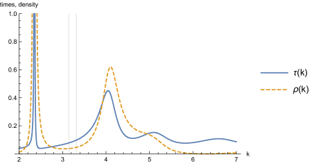
with tunneling times corresponding to real values of (i.e., ). Figure 1 shows a plot for the stationary transmission times , the distribution of wave numbers in the transmitted wave packet, and the distribution of wave numbers (momenta) in the incident packet, for two values of the barrier width. For the chosen parameters and barrier widths both the incident and the transmitted wave packets have an energy distribution very strongly peaked in a tunneling component (in the bottom plot of Figure 1 the barrier is much more opaque than that in the top plot and we can observe that – even if with a negligible probability for the parameters chosen for this plot – in this situation some above-the-barrier components start to appear in the distribution of the transmitted wave packet. So, in order to consider mainly transmission by tunneling we must restrict the barrier widths to not too large ones). We also observe the very well-known fact that the transmitted wave packet “speeds up” when compared to the incident particle Lunardi et al. (2011b). As a general rule, the larger is the barrier width (i.e., the more opaque is the barrier), the greater is the translation of the central component towards higher momenta. In which concerns the off resonance stationary transmission time, it initially grows with the barrier width, and saturates for very opaque barriers (the Hartman effect); on the other hand, it presents peaks at resonant wave numbers that grows and narrows with the barrier width – for a detailed discussion see Lunardi et al. (2011b)).
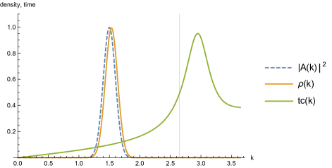
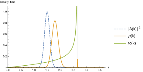
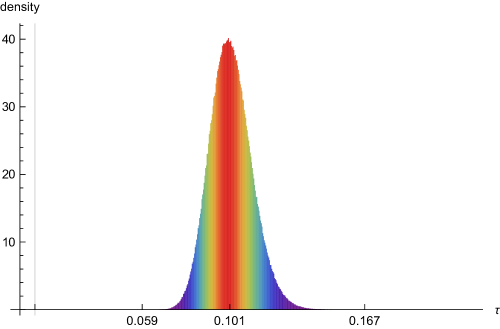
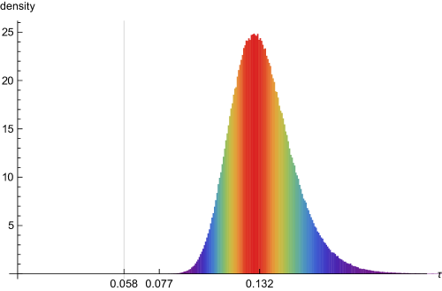
Figure 2 shows plots of the probability distribution of the tunneling times according to Equations (10)-(11), corresponding to both the barrier widths shown in the Figure 1 [to obtain these plots we used a Monte Carlo procedure to generate a large number of outcomes from the distribution , which afterwards were transformed into values by using the function ]. The vertical grey lines in these plots correspond to the time the light takes to cross the barrier distance. It is observed that for the two distributions shown in Figure 2 the probability to observe superluminal tunneling times is negligible. It is also observed that these distributions have a shape that resembles that of the distribution, albeit with a more pronounced skewness. This shape could be inferred from Figure 1 and from Equation (11), since grows very smoothly in the region were is non-vanishing. Furthermore, a comparison between the two plots in Figure 2 shows that the tunneling times do not grow linearly with the barrier width and, therefore, the distribution in the bottom plot of Figure 2 is “closer” to the light time than the distribution shown in the top plot; reference Lunardi et al. (2011b) already observed that for intermediate values of barrier widths the average transmission time – corresponding to the mean of the distribution – reaches a plateau.
V Distribution of ionization tunneling times
In this Section we obtain a distribution for tunneling times for a particle that is initially in a bound state of a given binding potential. The potential is then suddenly deformed in such a way that the particle can escape from the initially confining region by tunneling. The model considered here is a slight modification of that proposed by Ban et al. Ban et al. (2010) to simulate, in a simple scenario, key features of the decay of a localized state by tunneling ionization induced by the application of a strong external field with a finite duration.
In Ban et al. (2010), for , the particle is in an eigenstate of a semi-infinite square-well potential ,
| (16) |
and, therefore, it cannot decay by tunneling. At the potential is suddenly deformed to ,
| (17) |
such that the particle can now tunnel through the potential barrier – it is assumed that the wave function does not change during the sudden change of the potential. Finally, after a finite time the potential returns to its original configuration, , and tunneling terminates. The cutoff time mimics the natural upper bound for tunneling times measured in recent attoclock experiments (see, e.g., Landsman et al. (2014); Zimmermann et al. (2016) and references therein), since the opening and closing of the tunneling channel in these experiments occurs in intervals of half the laser field’s period.
Here, we deviate from Ban et al. (2010) by setting , i.e., once deformed the potential does not return to its original form and, after a long enough time, the particle will be transmitted with unit probability – thus, by eliminating the cutoff (which is just an experimental limitation) we are able to explore the whole range of possibilities for the ionization tunneling time. In addition, for , the particle is assumed to be coupled to a SWP quantum clock running only in the region , so that the clock’s readings for the asymptotic transmitted wave packet give the time the particle spent within the barrier after . Following Ban et al. (2010), we assume that for the particle is in the ground state of the potential , whose stationary wave function is given by
| (18) |
where is a normalization constant, , is the ground state energy, and . It is also assumed, as in Ban et al. (2010), that immediately after the sudden deformation of the potential from to , at , the wave function does not change. However, for the particle state, which is no longer an energy eigenstate, is given by a superposition of the energy eigenstates () of the potential , i.e., Ban et al. (2010)
| (19) |
where
with
| (20) |
where and the coefficients and the phase are determined by the usual boundary conditions at and , and are such that the normalization holds Ban et al. (2010). From the above expressions it follows that, without any loss of generality, we can take and all the eigenfunctions (20) to be real.
In order to consider the coupling with the SWP clock for times we proceed as follows. At the system particle+clock is described by the product state , where is the state (19) and is the initial clock state given by (3). After the particle and the clock states become entangled. For the procedure of post selection of the asymptotically transmitted wave function we notice that the role of the transmission coefficient for the wave function (20) is played by , where the superscript indicates the weak coupling with the clock. The right moving asymptotic wave packet representing the coupled system formed by the transmitted particle and the clock is
where, as before, [with quantities without the subscript “” representing the limit ]. By following the same steps described in reference Lunardi et al. (2011b), we trace out the clock’s degree of freedom in the asymptotic transmitted wave packet in order to obtain the distribution of the wave numbers for the asymptotically transmitted wave packet, which in this case is simply given by
| (21) |
i.e., the probability to find a wave number in the asymptotic transmitted wave packet is the same as in the initial state, which is as expected, since after a long enough time the initial wave packet will be transmitted with probability unit, as mentioned earlier.
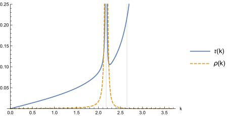
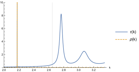
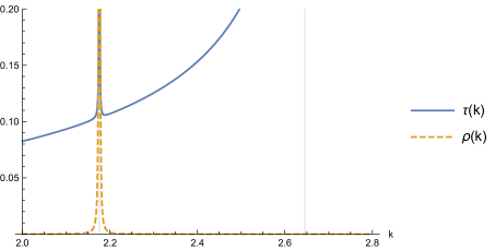
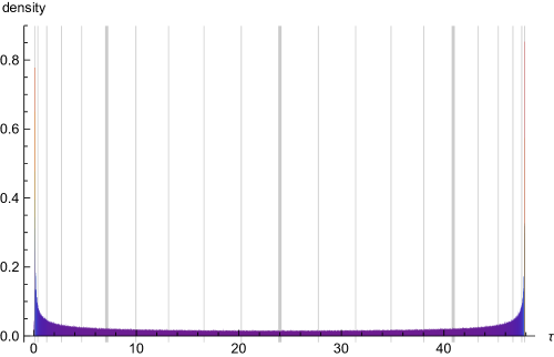
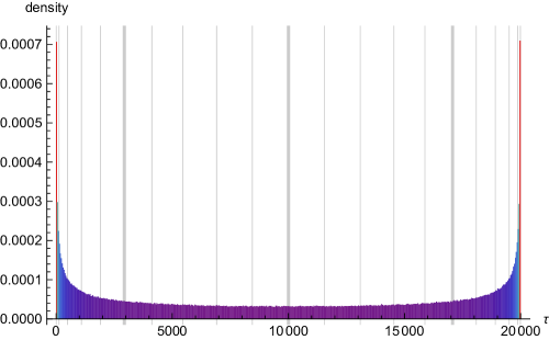
The general behavior of and is illustrated in Figures 3 and 4, corresponding to two barriers with different opacities ( and , respectively). These plots show, as expected, that the distribution is strongly peaked at the wave number , corresponding to the energy of the initially bound state, and is negligible for non-tunneling components. For tunneling wave numbers () the function is also strongly peaked at the same wave number , which corresponds to a local maximum (for non tunneling wave numbers there are several other resonance peaks). From Equation (11) we would expect that the peaks in the tunneling times distribution would occur for times corresponding to values of for which – which occur at points of local maxima and minima of the function – and corresponding to non-negligible . Therefore, from the plots in Figures 3 and 4 one could expect the first peak of the tunneling time distribution at (the local minimum of , which is similar for both barrier widths, since non-resonant times change little with the barrier width for opaque barriers, as is the case in Figures 3 and 4); a second peak in is expected to occur around the local maximum of , which corresponds to (this local maximum – corresponding to resonant wave numbers – changes significantly with the barrier widths, see, e.g., Lunardi et al. (2011b)). On the other hand, peaks in coming from local maxima (resonances) and minima associated with non-tunneling values of are suppressed, since in these cases. Figure 5 confirm these claims. For both barrier widths considered, the distribution of tunneling times is “U” shaped, having peaks at the times corresponding to the local maxima and minima of the stationary time inside the tunneling region. It should be observed that the larger is the barrier width, the broader is the tunneling time distribution, due to the strong increase of the resonant tunneling time with the barrier width.
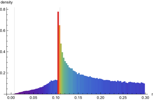
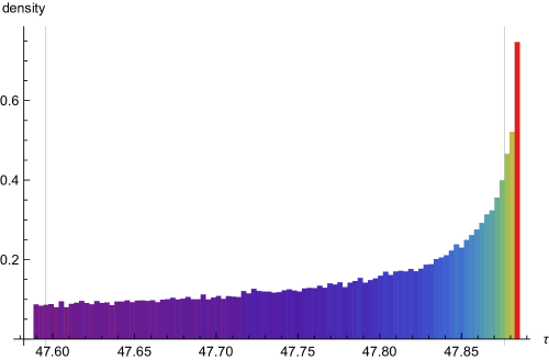
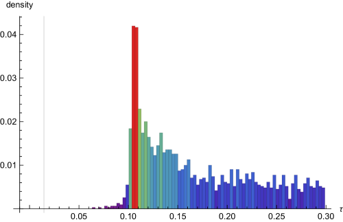
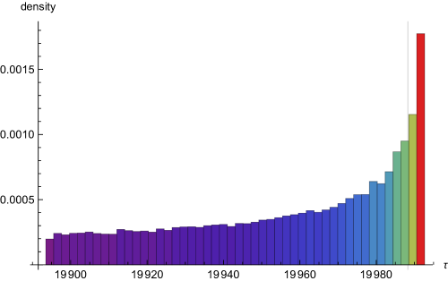
Figures 6 and 7 show close views of the tunneling time distributions for small and large tunneling times (Figure 6 corresponds to the plot at the top of Figure 5, whilst Figure 7 corresponds to the plot at the bottom of Figure 5). In the top plots of these Figures we can clearly observe the first peak around the local minimum of in the tunneling region, which in both plots corresponds to almost the same value attoseconds. The top plot of Figure 6 shows that for the less opaque barrier there exists a (very small) probability to observe a superluminal tunneling time. Even if this possibility cannot be precluded in principle, (see, e.g., Lunardi et al. (2011a)), in the present case the possibility of emergence of such small times was expected, since at there was a significant portion of the wave packet (roughly ) penetrating the whole distance of the barrier, and this has an important contribution to the emergence of small times in the clock’s readings associated to the transmitted particle. On the other hand, the top plot of Figure 7 shows that for the thicker barrier the probability for superluminal times is negligible – the portion of the wave packet already inside the barrier at is the same (), but the wave packet penetrates proportionally a smaller distance inside the barrier and, thus, it does not contribute in a significant way to the emergence of very small times in the clock readings. We note that the introduction of the cutoff , as in Ban et al. (2010), would result in a time distribution similar to the truncated distributions shown in the top plots of Figures 6 and 7.
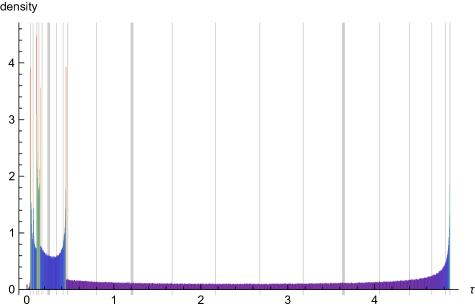
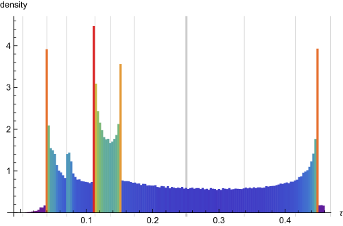
It is also worth to observe that, for small times, the distributions obtained here resemble qualitatively those in Figure 4 of Landsman et al. (2014), except for the presence of several peaks at discrete values of the time in the latter. The considerations above, relating the peaks of the distribution of clock times to the local maxima and minima of the stationary time and the magnitude of distribution in the neighborhood of these points, suggest a scenario in which such multiple peaks at discrete values of time can appear in the distribution of transmission times. Indeed, if above-the-barrier wave numbers had a significant contribution to the initial wave packet, then the several local maxima and minima present in the vicinities of the resonant non tunneling components will also contribute in a significant way to build multiple peaks in the distribution of transmission times; these peaks, however, could not be associated with the tunneling process. We can consider such a scenario by choosing as the initial state a tightly localized state given by , with and the barrier parameters , and , in Rydberg atomic units. In this situation the initial wave function is perfectly confined to the left of the barrier (), and above-the-barrier components contribute in a significant way to build the wave packet, as can be seen from in the top plot of Figure 8 (in this case the probability of finding a non tunneling component in the wave packet is approximately ). In this plot we can also observe that all the local maxima and minima of shown occur in neighborhoods of wave numbers for which is non-negligible; therefore, all these local maxima and minima contribute significantly to build multiple peaks in the distribution of transmission times . The middle and the bottom plots of Figure 8 confirm this statement: all the peaks of the distribution of transmission times correspond very closely to the local maxima and minima of , as can be seen by comparing the plots in the top and the bottom of this Figure (except for the first, all the other significant peaks in the bottom plot are associated to non-tunneling components).

VI Conclusions
Taking as a starting point the probabilistic (average) tunneling time obtained in Lunardi et al. (2011b) with the use of a SWP clock Salecker and Wigner (1958); Peres (1980); Calçada et al. (2009), we obtained a probability distribution of times, equations (10)-(11). An important advantage of using the SWP clock, in addition to those already mentioned, is that by running only when the particle is inside the barrier it allows us to address the concept of tunneling time in a proper way, since the time spent by the particle standing in the well before penetrating the barrier is not computed. A clear advantage of having a probability distribution of transmission (tunneling) times is that in addition to the usual expectation value, we can obtain all the statistical properties of this time, such as its most probable values (peaks of the distribution), the dispersion around the mean value, and the probability to observe extreme outcomes (superluminal times, for instance).
As an initial test, the distribution of times (10)-(11) was applied to the simple problem of a particle tunneling through a rectangular barrier. Unsurprisingly, it revealed behavior similar to that already known from previous works using a distribution of wave numbers (momentum) – see, e.g., Lunardi et al. (2011b) – although, using these conclusions are much more transparent. For example, one could answer the question about the possibility of superluminal tunneling by direct calculation from the probability distribution . In the non stationary case – which is the correct to address this question – this problem is usually answered by considering just the average tunneling time. But, given its probabilistic nature, an answer based only on the average time may not be satisfactory, especially if the dispersion of the distribution of tunneling times is large, which is often the case when one deals with well-localized particles, as suggested by the two situations addressed in the present work.
As a main application of (10)-(11), we considered a slight modification of the problem considered in Ban et al. (2010) to model strong field ionization by tunneling. The modification considered here was the elimination of the cutoff time that was introduced in Ban et al. (2010) to simulate the upper bound that arises in attoclock experiments Landsman et al. (2014); Zimmermann et al. (2016) due to the opening and closing of the tunneling channel, naturally associated with the oscillations in the laser field intensity. This cutoff is not a fundamental requirement, but rather it is associated to the experimental methods employed – in any case, its implementation is rather trivial, since it just truncates the distribution of times. The consideration of the full range of the distribution of times allowed us to show that an important contribution to comes from very large times associated with the resonance peaks in the tunneling region – these very long tunneling times occur with a probability comparable to very short ones, thus having an important impact on the average tunneling times and, therefore, cause difficulties when comparing theoretical predictions based on an average time with the outcomes of experiments presenting a natural cutoff in the possible time measurements. In particular, in the attoclock experiments the relevant measure is often associated to the peak of the tunneling time, which may be promptly identified once one knows the probability distribution for all possible times. A remark is in place, the distribution of times proposed here, built on the SWP clock readings, refers to the time the particle dwells within the barrier, while the tunneling times often measured in recent attoclock experiments actually refers to exit times Teeny et al. (2016).
In sum, the approach introduced above and resulting in (10)-(11) builds upon the already (conceptually) well tested SWP clock to provide a real-valued distribution of times that, in the simple models considered here, was demonstrated to have physically sound properties and, in fact, (rough) similarities with the time distribution obtained in recent experiments Landsman et al. (2014), therefore warrantying further investigation with more realistic potentials.
References
- Winful (2006a) H. G. Winful, Physics Reports 436, 1 (2006a).
- Winful (2006b) H. G. Winful, New Journal of Physics 8, 101 (2006b).
- Landsman et al. (2014) A. S. Landsman, M. Weger, J. Maurer, R. Boge, A. Ludwig, S. Heuser, C. Cirelli, L. Gallmann, and U. Keller, Optica 1, 343 (2014).
- Torlina et al. (2015) L. Torlina, F. Morales, J. Kaushal, I. Ivanov, A. Kheifets, A. Zielinski, A. Scrinzi, H. G. Muller, S. Sukiasyan, M. Ivanov, and O. Smirnova, Nature Physics 11, 503 (2015).
- Pedatzur et al. (2015) O. Pedatzur, G. Orenstein, V. Serbinenko, H. Soifer, B. D. Bruner, A. J. Uzan, D. S. Brambila, A. G. Harvey, L. Torlina, F. Morales, O. Smirnova, and N. Dudovich, Nature Physics 11, 815 (2015).
- Zimmermann et al. (2016) T. Zimmermann, S. Mishra, B. R. Doran, D. F. Gordon, and A. S. Landsman, Phys. Rev. Lett. 116, 233603 (2016).
- Chiao et al. (1991) R. Chiao, P. Kwiat, and A. Steinberg, Physica B: Condensed Matter 175, 257 (1991).
- Steinberg et al. (1993) A. M. Steinberg, P. G. Kwiat, and R. Y. Chiao, Phys. Rev. Lett. 71, 708 (1993).
- (9) L. C.R. and S. M. R., Annalen der Physik 7, 662.
- Krekora et al. (2001) P. Krekora, Q. Su, and R. Grobe, Phys. Rev. A 63, 032107 (2001).
- (11) L. C‐F. and C. X., Annalen der Physik 11, 916.
- Petrillo and Janner (2003) V. Petrillo and D. Janner, Phys. Rev. A 67, 012110 (2003).
- Chen and Li (2003) X. Chen and C.-F. Li, Phys. Rev. A 68, 052105 (2003).
- De Leo and Rotelli (2007) S. De Leo and P. Rotelli, The European Physical Journal C 51, 241 (2007).
- Lunardi and Manzoni (2007) J. T. Lunardi and L. A. Manzoni, Physical Review A 76, 042111 (2007).
- Lunardi et al. (2011a) J. T. Lunardi, L. A. Manzoni, A. T. Nystrom, and B. M. Perreault, Journal of Russian Laser Research 32, 431 (2011a).
- Peres (1980) A. Peres, American Journal of Physics 48, 552 (1980).
- Wigner (1955) E. P. Wigner, Physical Review 98, 145 (1955).
- Smith (1960) F. T. Smith, Physical Review 118, 349 (1960).
- Baz’ (1967) A. I. Baz’, Soviet Journal of Nuclear Physics 4, 182 (1967).
- Rybachenko (1967) V. F. Rybachenko, Soviet Journal of Nuclear Physics 5, 635 (1967).
- Büttiker (1983) M. Büttiker, Physical Review B 27, 6178 (1983).
- Falck and Hauge (1988) J. P. Falck and E. H. Hauge, Physical Review B 38, 3287 (1988).
- Salecker and Wigner (1958) H. Salecker and E. P. Wigner, Physical Review 109, 571 (1958).
- Eckle et al. (2008) P. Eckle, A. N. Pfeiffer, C. Cirelli, A. Staudte, R. Dörner, H. G. Muller, M. Büttiker, and U. Keller, Science 322, 1525 (2008).
- Orlando et al. (2014) G. Orlando, C. R. McDonald, N. H. Protik, G. Vampa, and T. Brabec, Journal of Physics B: Atomic, Molecular and Optical Physics 47, 204002 (2014).
- Landsman and Keller (2015) A. S. Landsman and U. Keller, Physics Reports 547, 1 (2015).
- Lunardi et al. (2011b) J. T. Lunardi, L. A. Manzoni, and A. T. Nystrom, Physics Letters A 375, 415 (2011b).
- Kelkar et al. (2009) N. G. Kelkar, H. M. Castañeda, and M. Nowakowski, EPL (Europhysics Letters) 85, 20006 (2009).
- Goto et al. (2004) M. Goto, H. Iwamoto, V. M. de Aquino, V. C. Aguilera-Navarro, and D. H. Kobe, Journal of Physics A: Mathematical and General 37, 3599 (2004).
- Brouard et al. (1994) S. Brouard, R. Sala, and J. G. Muga, Phys. Rev. A 49, 4312 (1994).
- Petrillo and Olkhovsky (2006) V. Petrillo and V. S. Olkhovsky, EPL (Europhysics Letters) 74, 327 (2006).
- Hartman (1962) T. E. Hartman, Journal of Applied Physics 33, 3427 (1962).
- Frentz et al. (2014) B. A. Frentz, J. T. Lunardi, and L. A. Manzoni, European Physical Journal Plus 129, 5 (2014).
- Turok (2014) N. Turok, New Journal of Physics 16, 063006 (2014).
- Ban et al. (2010) Y. Ban, E. Y. Sherman, J. G. Muga, and M. Büttiker, Phys. Rev. A 82, 062121 (2010).
- Calçada et al. (2009) M. Calçada, J. T. Lunardi, and L. A. Manzoni, Physical Review A 79, 012110 (2009).
-
Note (1)
Specifically, we use the fact that
where is the set of zeros of the function and the prime indicates a derivative with respect to the independent variable. - Park (2011) C.-S. Park, Physics Letters A 375, 3348 (2011).
- Park (2009) C.-S. Park, Physical Review A 80, 012111 (2009).
- Aharonov et al. (2002) Y. Aharonov, N. Erez, and B. Reznik, Physical Review A 65, 052124 (2002).
- Aharonov et al. (2003) Y. Aharonov, N. Erez, and B. Reznik, Journal of Modern Optics 50, 1139 (2003).
- Lee et al. (2016) M. A. Lee, J. T. Lunardi, L. A. Manzoni, and E. A. Nyquist, Frontiers in Physics 4, 10 (2016).
- Teeny et al. (2016) N. Teeny, E. Yakaboylu, H. Bauke, and C. H. Keitel, Phys. Rev. Lett. 116, 063003 (2016).