A Chebyshev-based rectangular-polar integral solver for scattering by general geometries described by non-overlapping patches

Abstract

This paper introduces a high-order-accurate strategy for integration of singular kernels and edge-singular integral densities that appear in the context of boundary integral equation formulations of the problem of acoustic scattering. In particular, the proposed method is designed for use in conjunction with geometry descriptions given by a set of arbitrary non-overlapping logically-quadrilateral patches—which makes the algorithm particularly well suited for treatment of CAD-generated geometries. Fejér’s first quadrature rule is incorporated in the algorithm, to provide a spectrally accurate method for evaluation of contributions from far integration regions, while highly-accurate precomputations of singular and near-singular integrals over certain “surface patches” together with two-dimensional Chebyshev transforms and suitable surface-varying “rectangular-polar” changes of variables, are used to obtain the contributions for singular and near-singular interactions. The overall integration method is then used in conjunction with the linear-algebra solver GMRES to produce solutions for sound-soft open- and closed-surface scattering obstacles, including an application to an aircraft described by means of a CAD representation. The approach is robust, fast, and highly accurate: use of a few points per wavelength suffices for the algorithm to produce far-field accuracies of a fraction of a percent, and slight increases in the discretization densities give rise to significant accuracy improvements.

1 Introduction

The solution of scattering problems by means of boundary integral representations has proven to be a game-changer when the ratio of volume to surface scattering is large, where volumetric solvers become intractable due to memory requirements and computational cost. At the heart of every boundary integral equation (BIE) solver lies an integration strategy that must be able to handle the weakly singular integrals associated with the Green-function integral formulations of acoustic and electromagnetic scattering. Several approaches have been proposed to deal with this difficulty, most notably those put forward in [5, 13, 2].

For three-dimensional scattering, which reduces to two-dimensional integral equations along the scatterer’s surface, there is no simple quadrature rule that accurately evaluates the weakly singular scattering kernels, which makes the three-dimensional problem considerably more difficult than its two dimensional counterpart—for which a closed form expression exists for the integrals of the product of certain elementary singular kernels and complex exponentials [11]. Therefore, a number of approaches have been proposed to treat these integrals—which can be classified into the Nyström, collocation and Galerkin categories [11]. Nyström methods use a quadrature rule to evaluate integrals, which leads to a system of linear equations; the collocation approach finds a solution on a finite-dimensional space which satisfies the continuous BIE at some collocation points (hence the name); the Galerkin approach solves the BIE in the weak formulation using finite-element spaces for both the solution and test functions.

In this contribution, we present what can be considered as a hybrid Nyström-collocation method, in which the far interactions are computed via Fejér’s fist quadrature rule (Nyström), which yields spectrally accurate results for smooth integrands, while the integrals involving singular and near-singular kernels are obtained by relying on highly-accurate precomputations of the kernels times Chebyshev polynomials (which are produced by means of a surface-varying rectangular-polar change of variables), together with Chebyshev expansions of the densities (collocation). The derivatives of the rectangular-polar change of variables vanish at the kernel singularity (the surface-varying observation point) and geometric-singularity points, producing a “floating” clustering around those points which gives rise to high-order accuracy. This change of variables is analogous to that of the polar integration in [5], but differs in the fact that it is applied on a rectangular mesh, hence the “rectangular-polar” terminology we use to refer to this methodology. The sinh transform [16, 15] was also tested as an alternative to the change of variables we eventually selected: the latter method was preferred as the sinh change of variable does not appear to allow sufficient control on the distribution of discretization points along the integration mesh, which is needed in order to accurately resolve the wavelength without use of excessive numbers of discretization points.

The proposed rectangular-polar approach, which yields high-order accuracy, leads to several additional desirable properties, such as the use of Chebyshev representations for the density, which allows the possibility to compute differential geometry quantities needed for electromagnetic BIE by means differentiation of Chebyshev series. Additionally, the nodes for Fejér’s first quadrature are the same as the nodes for the discrete orthogonality property of Chebyshev polynomials, which make the computation of the Chebyshev transforms straightforward. In addition to scattering by a bounded obstacle, this integral equation solver can also be used in the context of the Windowed Green function method for scattering by unbounded obstacles, as is the case of layered media [8, 10, 19] and waveguide problems [4].

This paper is organized as follows. Section 2 states the mathematical problem of acoustic scattering and the integral representations used in this paper. Section 3 then describes the overall rectangular-polar integration strategy, including details concerning the methodologies used to produce integrals for smooth, singular and near-singular kernels as well as edge-singular integral densities. A variety of numerical results for open and closed scattering surfaces are then presented in Section 4, emphasizing on the convergence properties of both the forward map (which evaluates the action of the integral operator for a given density) as well as the full scattering solver, and demonstrating the accuracy, generality, and speed of the proposed approach. Results of an application to a problem of scattering by a geometry generated by CAD software is also presented in this section, demonstrating the applicability to complex geometrical designs in science and engineering. Section 5, finally, presents a few concluding remarks.

2 Preliminaries

For conciseness, we consider the problem of acoustic scattering by a sound-soft obstacle, though the methodology proposed is also applicable to electromagnetic scattering and other integral-equation problems involving singular kernels.

Let $\Omega$ denote the complement of an obstacle $D$ in three-dimensional space, and let $\Gamma$ denote the boundary of the obstacle. Calling $U$, $U^{\text{scat}}$ and $U^{\text{inc}}$ the total, scattered and incident fields respectively, then $U=U^{\text{scat}}+U^{\text{inc}}$ obeys the Helmholtz equation

$$\Delta U(\boldsymbol{r})+k^{2}U(\boldsymbol{r})=0,\quad\boldsymbol{r}\in\mathbb{R}^{3}\setminus\overline{\Gamma},$$ (1)

with wavenumber $k=2\pi/\lambda$, and the scattered field $U^{\text{scat}}$ satisfies the Sommerfeld radiation condition and the boundary condition

$$U^{\text{scat}}(\boldsymbol{r})=-U^{\text{inc}}(\boldsymbol{r}),\quad\boldsymbol{r}\in\Gamma.$$ (2)

As it is well known [11], the scattered field can be represented in terms of layer potentials, reducing the problem to a boundary integral equation with singular kernels. The single- and double-layer potentials are defined by

$$\mathscr{S}[\,\widetilde{\varphi}\,](\boldsymbol{r}) =\int_{\Gamma}G(\boldsymbol{r},\boldsymbol{r}^{\prime})\,\widetilde{\varphi}\,(\boldsymbol{r}^{\prime})\text{d}\sigma(\boldsymbol{r}^{\prime}),\quad\boldsymbol{r}\in\mathbb{R}^{3}\setminus\overline{\Gamma},$$ (3)

$$\mathscr{D}[\,\widetilde{\varphi}\,](\boldsymbol{r}) =\int_{\Gamma}\frac{\partial G(\boldsymbol{r},\boldsymbol{r}^{\prime})}{\partial\boldsymbol{n}(\boldsymbol{r}^{\prime})}\,\widetilde{\varphi}\,(\boldsymbol{r}^{\prime})\text{d}\sigma(\boldsymbol{r}^{\prime}),\quad\boldsymbol{r}\in\mathbb{R}^{3}\setminus\overline{\Gamma},$$ (4)

respectively, and where $G(\boldsymbol{r},\boldsymbol{r}^{\prime})=\exp{(ik|\boldsymbol{r}-\boldsymbol{r}^{\prime}|)}/(4\pi|\boldsymbol{r}-\boldsymbol{r}^{\prime}|)$ is the free-space Green function of the Helmholtz equation, $\boldsymbol{n}$ is the outwards-pointing normal vector, and $\,\widetilde{\varphi}\,$ is the surface density. In this paper, we demonstrate the proposed methodology by considering two problems under a unified scheme, namely the case of closed and open surfaces.

2.1 Closed surfaces

For the case of a closed, bounded obstacle, we use a standard combined-field formulation [11]

$$U^{\text{scat}}(\boldsymbol{r})=\mathscr{D}[\,\widetilde{\varphi}\,](\boldsymbol{r})-ik\mathscr{S}[\,\widetilde{\varphi}\,](\boldsymbol{r}),\quad\boldsymbol{r}\in\mathbb{R}^{3}\setminus\overline{\Gamma},$$ (5)

which leads to the second-kind integral equation at the boundary

$$\displaystyle\frac{1}{2}\,\widetilde{\varphi}\,(\boldsymbol{r})+D[\,\widetilde{\varphi}\,](\boldsymbol{r})-ikS[\,\widetilde{\varphi}\,](\boldsymbol{r})=-U^{\text{inc}}(\boldsymbol{r}),\quad\boldsymbol{r}\in\Gamma,$$ (6)

where the single- and double-layer boundary operators are defined as

$$\displaystyle S[\,\widetilde{\varphi}\,](\boldsymbol{r}) =\int_{\Gamma}G(\boldsymbol{r},\boldsymbol{r}^{\prime})\,\widetilde{\varphi}\,(\boldsymbol{r}^{\prime})\text{d}\sigma(\boldsymbol{r}^{\prime}),\quad\boldsymbol{r}\in\Gamma,$$ (7)

$$\displaystyle D[\,\widetilde{\varphi}\,](\boldsymbol{r}) =\int_{\Gamma}\frac{\partial G(\boldsymbol{r},\boldsymbol{r}^{\prime})}{\partial\boldsymbol{n}(\boldsymbol{r}^{\prime})}\,\widetilde{\varphi}\,(\boldsymbol{r}^{\prime})\text{d}\sigma(\boldsymbol{r}^{\prime}),\quad\boldsymbol{r}\in\Gamma,$$ (8)

respectively.

This formulation is guaranteed to provide a unique density solution to the scattering problem considered here [11], and due to the nature of this second-kind integral equation, the number of iterations for GMRES remains essentially bounded as $k$ is increased.

2.2 Open surfaces

For scattering by an open surface, a combined field formulation is not possible given that the jump conditions of the double-layer would imply different field values from above and below the open surface. However, one can use a single-layer formulation for such purpose, in this case we have

$$U^{\text{scat}}(\boldsymbol{r})=\mathscr{S}[\,\widetilde{\varphi}\,](\boldsymbol{r}),\quad\boldsymbol{r}\in\mathbb{R}^{3}\setminus\overline{\Gamma},$$ (9)

which leads to a first-kind integral equation

$$\displaystyle S[\,\widetilde{\varphi}\,](\boldsymbol{r})=-U^{\text{inc}}(\boldsymbol{r}),\quad\boldsymbol{r}\in\Gamma.$$ (10)

It is known that this formulation leads to an ill-conditioned system, which manifests in increasing number of iterations for GMRES as $k$ becomes larger. For the purpose of clarity, we choose to use this simple formulation to present the open-surface scattering solver, which, as it will be shown in Section 4.3, was enough to achieve accuracies up to $10^{-13}$ in the far field solutions for relatively low wavenumbers. For higher frequency problems where the computational time may be a severe constrain, a regularized version of this solver can be obtained by means of a composition of the single-layer operator with the derivative of the double-layer, see [7, Sec. 3].

An important aspect of the open-surface case that leads to significant difficulties is that the solution $\,\widetilde{\varphi}\,(\boldsymbol{r})$ presents a singularity of the form

$$\,\widetilde{\varphi}\,\sim\frac{\Phi}{\sqrt{d}},$$ (11)

where $d$ is the distance to the edge and $\Phi$ is an infinitely differentiable function throughout the boundary (including the edge) [7]. In [7], a strategy based on quadrature rules for the exact singularity form where introduced, together with the polar integration method from [5]. We propose an alternative approach in which, in addition of the polar-rectangular setup, a change of variables is introduced in the parametrization of the surface. This change of variables is such that its derivatives vanish at the edges, and thus smooths out the integrands. Although not particularly designed to exactly match the singularity of the density at edges, the proposed algorithm does provide a robust approach for the treatment of the density-singularities that arise in the closed-surface edge case (for which the degree of the singularity depends on the edge angle, which may itself vary along the edge).

2.3 Surface representation

The proposed method assumes the scattering surface is described by a set of $M$ non-overlapping “logically-quadrilateral” (LQ) parametrized patches. This geometrical description is particularly well suited for designs generated by CAD software, which generally can export surface representations in terms of NURBS-based models—that is, parametrizations expressed in terms of certain types of Rational B-Splines. In fact, the potential afforded by direct use of CAD-exported representations (without the expense, difficulty and accuracy deterioration inherent in the use of surface triangulations) provided the driving force leading to this paper: each NURBS trimmed surface can be “quadrilateralized” without great difficulty, which lends the method essentially complete geometric generality and a remarkable ease of use.

In the proposed approach, then, the scattering surface $\Gamma$ is partitioned on the basis of a finite number $M$ of parametrizations

$$\widetilde{\boldsymbol{r}}^{\,q}:[-1,1]^{2}\to\mathbb{R}^{3}\quad(q=1,2,\dots,M),$$

each one of which maps the unit square $[-1,1]^{2}$ in the $(s,t)$-plane onto an LQ patch within $\Gamma$. Since we require the system of LQ patches to cover $\Gamma$, we have, in particular

$$\displaystyle\Gamma=\bigcup_{q=1}^{M}\left\{\widetilde{\boldsymbol{r}}^{\,q}(s,t)\;\big{|}\;(s,t)\in[-1,1]^{2}\right\}.$$ (12)

Clearly, any integral over $\Gamma$ can be decomposed as a sum of integrals over each of the patches. With the goal of treating the closed- and open-surface cases in a unified way, we define the boundary integrals

$$I(\boldsymbol{r}) =\sum_{q=1}^{M}I^{q}(\boldsymbol{r}),$$ (13)

$$I^{q}(\boldsymbol{r}) =\int_{\Gamma^{q}}\widetilde{\operatorname{H}}(\boldsymbol{r},\boldsymbol{r}^{\prime})\,\widetilde{\varphi}\,(\boldsymbol{r}^{\prime})\text{d}\sigma(\boldsymbol{r}^{\prime}),$$ (14)

where

$$\displaystyle\widetilde{\operatorname{H}}(\boldsymbol{r},\boldsymbol{r}^{\prime})=\begin{cases}\displaystyle\frac{\partial G(\boldsymbol{r},\boldsymbol{r}^{\prime})}{\partial\boldsymbol{n}(\boldsymbol{r}^{\prime})}-ikG(\boldsymbol{r},\boldsymbol{r}^{\prime}),&\text{(Closed surface)},\\ \displaystyle G(\boldsymbol{r},\boldsymbol{r}^{\prime}),&\text{(Open surface)}.\end{cases}$$ (15)

In the following section, we propose a methodology for accurate evaluation of the integrals $I^{q}(\boldsymbol{r})$ for a given density $\,\widetilde{\varphi}\,(\boldsymbol{r}^{\prime})$. The solution to the integral equation problem is then obtained via an application of the iterative linear-algebra solver GMRES.

3 Integration strategy

The integration scheme we present consists of three main components: (1) Use of Fejér’s first quadrature rule to compute integrals between patches that are “far” away from each other, (2) A rectangular-polar high-order accurate quadrature rule for self-patch and near-patch singular integrals, and (3) A change of variables that resolves the density singularities that arise at edges.

Using, for each $q$, the parametrization $\widetilde{\boldsymbol{r}}^{\,q}$, the integral (14) can be expressed in the form

$$I^{q}(\boldsymbol{r}) =\int_{-1}^{1}\int_{-1}^{1}\widetilde{\operatorname{H}}^{q}(\boldsymbol{r},s,t)\widetilde{J}^{q}(s,t)\widetilde{\varphi}^{q}(s,t)\text{d}s\>\text{d}t,\quad(\boldsymbol{r}\in\Gamma),$$ (16)

where $\widetilde{J}^{q}(s,t)$ denotes the surface Jacobian, and where

$$\displaystyle\widetilde{\operatorname{H}}^{q}(\boldsymbol{r},s,t) =\widetilde{\operatorname{H}}\left(\boldsymbol{r},\widetilde{\boldsymbol{r}}^{\,q}(s,t)\right),$$ (17)

$$\widetilde{\varphi}^{q}(s,t) =\,\widetilde{\varphi}\,\left(\widetilde{\boldsymbol{r}}^{\,q}(s,t)\right).$$ (18)

The strategy proposed for evaluation of the integral in equation (16) depends on the proximity of the point $\boldsymbol{r}$ to the $q$-th patch. For points $\boldsymbol{r}$ that are “far” from the patch, Fejér’s first quadrature rule is used as detailed in Section 3.2. A special technique, the rectangular-polar method, is then presented in Section 3.3 to treat the case in which $\boldsymbol{r}$ is “close” or within the $q$-th patch. Before the presentation of these smooth, singular and near-singular integration methods, Section 3.1 describes the singular character of integral-equation densities at edges, and proposes a methodology, which is incorporated in the subsequent sections, for their treatment in a high-order accurate fashion.

3.1 Density singularities along edges

The sharp edges encountered in general geometric designs have provided a persistent source of difficulties to integral equation methods and other scattering solvers. The presence of such edges leads to integrable singularities in the density solutions in both the open-surface [7] and closed-surface [12, 17] cases. The strength of the singularity, however, depends on the formulation and, for closed-surfaces, on the angle at the edge, which is generally not constant.

In order to tackle this difficulty in a general and robust manner, we introduce a change of variables on the parametrization variables $(s,t)$, a number of whose derivatives vanish along edges. Such changes of variables can be devised from mappings such as the one presented in [11, Sec. 3.5], which is given by

$$\displaystyle w(\tau)=2\pi\frac{[v(\tau)]^{p}}{[v(\tau)]^{p}+[v(2\pi-\tau)]^{p}},\quad 0\leq\tau\leq 2\pi,$$ (19)

where

$$\displaystyle v(\tau)=\left(\frac{1}{p}-\frac{1}{2}\right)\left(\frac{\pi-\tau}{\pi}\right)^{3}+\frac{1}{p}\left(\frac{\tau-\pi}{\pi}\right)+\frac{1}{2}.$$ (20)

It is easy to check that the derivatives of $w(\tau)$ up to order $p-1$ vanish at the endpoints. The function $w(\tau)$ can then be used to construct a change of variables to accurately resolve the edge singularities while mapping the interval $[-1,1]$ to itself. The change-of-variable mappings we use are given by

$$s={\eta_{s}^{\,q}}(u)=\begin{cases}u,&\text{No edge on }s\\ -1+\frac{1}{\pi}w\left(\pi[u+1]\right),&\text{Edges at }s\pm 1\\ -1+\frac{2}{\pi}w\left(\frac{\pi}{2}[u+1]\right),&\text{Edge at }s=-1\text{ only}\\ -3+\frac{2}{\pi}w\left(\pi+\frac{\pi}{2}[u+1]\right),&\text{Edge at }s=1\text{ only}\end{cases}$$ (21)

and similarly

$$t={\eta_{t}^{\,q}}(v)=\begin{cases}v,&\text{No edge on }t\\ -1+\frac{1}{\pi}w\left(\pi[v+1]\right),&\text{Edges at }t\pm 1\\ -1+\frac{2}{\pi}w\left(\frac{\pi}{2}[v+1]\right),&\text{Edge at }t=-1\text{ only}\\ -3+\frac{2}{\pi}w\left(\pi+\frac{\pi}{2}[v+1]\right),&\text{Edge at }t=1\text{ only}\end{cases}$$ (22)

Incorporating the change of variables (21) and (22), the integral in equation (16) becomes an integral in which a weakly singular kernel is applied to a finitely smooth function:

$$I^{q}(\boldsymbol{r}) =\int_{-1}^{1}\int_{-1}^{1}{\operatorname{H}}^{q}(\boldsymbol{r},u,v){J}^{q}(u,v)\frac{d{\eta_{s}^{\,q}}}{du}(u)\frac{d{\eta_{t}^{\,q}}}{dv}(v){\varphi}^{q}(u,v)\text{d}u\>\text{d}v,\quad\boldsymbol{r}\in\Gamma,$$ (23)

where

$$\displaystyle{\operatorname{H}}^{q}(\boldsymbol{r},u,v) =\widetilde{\operatorname{H}}^{q}\left(\boldsymbol{r},{\eta_{s}^{\,q}}(u),{\eta_{t}^{\,q}}(v)\right),$$ (24)

$${\varphi}^{q}(u,v) =\widetilde{\varphi}^{q}\left({\eta_{s}^{\,q}}(u),{\eta_{t}^{\,q}}(v)\right),$$ (25)

$$\boldsymbol{r}^{\,q}(u,v) =\widetilde{\boldsymbol{r}}^{\,q}\left({\eta_{s}^{\,q}}(u),{\eta_{t}^{\,q}}(v)\right),$$ (26)

$${J}^{q}(u,v) =\widetilde{J}^{q}(s,t).$$ (27)

(The edge-vanishing derivative factors in the integrand smooth-out any possible edge singularities in the density ${\varphi}^{q}$ [11].) The proposed algorithm evaluates such integrals by means of the “smooth-density methods” described in Sections 3.2 and 3.3 below.

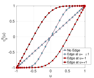
Figure 1: Change of variables (equations (21) and (22)) used to resolve the density edge-singularities.

3.2 Non-adjacent integration

The algorithm we use for the evaluation of the quantity $I^{q}(\boldsymbol{r})$, defined by (16), is based on the reformulation (23)—which takes into account all the possible ways in which edge-singularities may or may not appear within an integration patch. (The algorithm does assume that geometric singularities may only appear along patch boundaries.)

In the “non-adjacent” integration case considered in this section, in which the point $\boldsymbol{r}$ is far from the integration patch, the integrand in (23) is smooth—in view of the changes of variables inherent in that equation, which, in particular, give rise to edge-vanishing derivative factors that smooth-out any possible edge-singularity in the density ${\varphi}^{q}$ itself. (Using well known asymptotics of edge singularities it is easy to check [11, 9] that the vanishing derivatives indeed smooth out all possible edge singularities, to any desired order of smoothness, provided a sufficiently high value of $p$ is used. Values of $p$ as low as $p=2$ are often found to be adequately useful, for accuracies of the order of $1\%$, but values of $p$ of the orders of four to six or above can enable significantly faster convergence and lower computing costs for higher accuracies, as demonstrated e.g. in Figure 7.)

In view of the smoothness of the integrands for the non-adjacent cases considered presently ($\boldsymbol{r}$ is far from the integration patch), then, the integral in (23) could be accurately evaluated on the basis of any given high-order quadrature rule. Our implementation utilizes Fejér’s first quadrature rule [21], which effectively exploits the discrete orthogonality property satisfied by the Chebyshev polynomials in the Chebyshev meshes used, and which also allows for straightforward computation of the two-dimensional Chebyshev transforms that are required as part of the singular and near-singular integration algorithms described in Section 3.3.

For a discretization using $N$ points, the quadrature nodes and weights are given by

$$\displaystyle x_{j}=\cos{\left(\pi\frac{2j+1}{2N}\right)},\quad j=0,\dots,N-1,$$ (28)

$$\displaystyle w_{j}=\frac{2}{N}\left(1-2\sum_{\ell=1}^{\lfloor N/2\rfloor}\frac{1}{4\ell^{2}-1}\cos{(\ell x_{j})}\right),\quad j=0,\dots,N-1,$$ (29)

respectively. Then using the Cartesian-product discretization $\{u_{i}=x_{i}|i=0,\dots,{N_{u}^{\,q}}-1\}\times\{v_{j}=x_{j}|j=0,\dots,{N_{v}^{\,q}}-1\}$, the integral in (16) can be approximated by the quadrature expression

$$I^{q}(\boldsymbol{r})\approx\sum_{j=0}^{{N_{v}^{\,q}}-1}\sum_{i=0}^{{N_{u}^{\,q}}-1}{\operatorname{H}}^{q}(\boldsymbol{r},u_{i},v_{j}){J}^{q}(u_{i},v_{j})\frac{d{\eta_{s}^{\,q}}}{du}\frac{d{\eta_{t}^{\,q}}}{dv}w_{i}w_{j}\,{\varphi}^{q}(u_{i},v_{j}),\quad\boldsymbol{r}\in\Omega^{f}_{q}.$$ (30)

where $\Omega^{f}_{q}$ represents the set of points that are “sufficiently far” from the $q$-th integration patch.

3.3 Singular “rectangular-polar” integration algorithm and a new edge-resolved integral unknown

In this section we consider once again the problem of evaluation the quantity $I^{q}(\boldsymbol{r})$, on the basis of the reformulation (23), but this time (with reference to the last paragraph in Section 3.2) for points $\boldsymbol{r}$ that are not sufficiently far from the $q$-th integration patch. The set of all such points, which contains only points that either lie within the $q$-th patch or are “close” to it, will be denoted by $\Omega^{c}_{q}$. The problem of evaluation of $I^{q}$ for $\boldsymbol{r}\in\Omega^{c}_{q}$ presents a significant challenge in view of the singularity of the kernel $\widetilde{\operatorname{H}}(\boldsymbol{r},\boldsymbol{r}^{\prime})$ at $\boldsymbol{r}=\boldsymbol{r}^{\prime}$.

In order to deal with this difficulty, we propose once again the use of smoothing changes of variables: we will seek to incorporate in the integration process a change of variables whose derivatives vanish at the singularity or, for nearly singular problems, at the point in the $q$-th patch that is closest to the singularity. In previous implementations [5, 7], such changes of variables required interpolation of the density ${\varphi}^{q}$ from the fixed nodes $(u_{i},v_{j})$ to the new integration points. The interpolation step, though viable, can amount to a significant portion of the overall cost. We thus propose, instead, use of a precomputation scheme for which integrals of the kernel times Chebyshev polynomials are evaluated with high-accuracy. Since Chebyshev polynomials can easily be evaluated at any point in their domain of definition, this approach does not require an interpolation step. And, since these integrals are independent of the density, they need only be computed once at the beginning of any application of the algorithm, and reused in the algorithm as part of any necessary integration processes in subsequent linear-algebra (GMRES) iterations. Thus, for a given density ${\varphi}^{q}$ the overall quantity $I^{q}(\boldsymbol{r})$ with $\boldsymbol{r}\in\Omega^{c}_{q}$ can be computed by first obtaining the Chebyshev expansion

$$\psi^{q}(u,v)=\sum_{m=0}^{{N_{v}^{\,q}}-1}\sum_{n=0}^{{N_{u}^{\,q}}-1}a^{q}_{n,m}T_{n}(u)T_{m}(v),$$ (31)

of the modified edge-resolved (smooth) density

$$\psi^{q}(u,v)=\frac{d{\eta_{s}^{\,q}}}{du}(u)\frac{d{\eta_{t}^{\,q}}}{dv}(v){\varphi}^{q}(u,v),$$

and then applying the precomputed integrals for Chebyshev densities.

In detail, the necessary Chebyshev coefficients $a^{q}_{n,m}$ can be computed using the relation [20]

$$\displaystyle a^{q}_{n,m}=\frac{\alpha_{n}\alpha_{m}}{{N_{u}^{\,q}}{N_{v}^{\,q}}}\sum_{j=0}^{{N_{v}^{\,q}}-1}\sum_{i=0}^{{N_{u}^{\,q}}-1}\psi^{q}(u_{i},v_{j})T_{n}(u_{i})T_{m}(v_{j})$$ (32)

that results from the discrete-orthogonality property enjoyed by Chebyshev polynomials, where

$$\alpha_{n}=\begin{cases}1,&n=0,\\ 2,&n\neq 0.\end{cases}$$ (33)

As is well known, the Chebyshev coefficients $a^{q}_{n,m}$ can be computed in a fast manner either by means of the FFT algorithm or, for small expansion orders, by means of partial summation [1, Sec. 10.2]. In practice, relatively small orders and numbers of discretization points are used, and we thus opted for the partial summation strategy.

Using the expansion (31) we then obtain

$$\displaystyle I^{q}(\boldsymbol{r}) =\int_{-1}^{1}\int_{-1}^{1}{\operatorname{H}}^{q}(\boldsymbol{r},u,v){J}^{q}(u,v)\left(\sum_{m=0}^{{N_{v}^{\,q}}-1}\sum_{n=0}^{{N_{u}^{\,q}}-1}a^{q}_{n,m}T_{n}(u)T_{m}(v)\right)\text{d}u\>\text{d}v$$ (34)

from which, exchanging the integrals with the sum, it follows that

$$\displaystyle I^{q}(\boldsymbol{r})=\sum_{m=0}^{{N_{v}^{\,q}}-1}\sum_{n=0}^{{N_{u}^{\,q}}-1}a^{q}_{n,m}\int_{-1}^{1}\int_{-1}^{1}{\operatorname{H}}^{q}(\boldsymbol{r},u,v){J}^{q}(u,v)T_{n}(u)T_{m}(v)\,\text{d}u\>\text{d}v.$$ (35)

As mentioned above, the double integral is independent of the density, and therefore it only depends on the geometry, the kernel, and the target point $\boldsymbol{r}\in\Omega^{c}_{q}$. For the computation of the forward map, we only need to evaluate $I^{q}(\boldsymbol{r})$ for all discretization points $\boldsymbol{r}\in\Omega^{c}_{q}$. Thus, in the proposed strategy, the integral in (35) must be precomputed for each $q$ and for each combination of a target point $\boldsymbol{r}\in\Omega^{c}_{q}$ and a relevant product of Chebyshev polynomials. Denoting the set of all discretization points by

$$\displaystyle\chi=\left\{\widetilde{\boldsymbol{r}}^{\,q}\left({\eta_{s}^{\,q}}(u_{i}),{\eta_{t}^{\,q}}(v_{j})\right)\big{|}\;q=1,\dots,M,\;i=1,\dots,{N_{u}^{\,q}},\;j=1,\dots,{N_{v}^{\,q}}\right\},$$ (36)

and using the weights

$$\displaystyle\beta_{n,m}^{\,q,\ell}=\int_{-1}^{1}\int_{-1}^{1}{\operatorname{H}}^{q}(\boldsymbol{r}_{\ell},u,v){J}^{q}(u,v)T_{n}(u)T_{m}(v)\,\text{d}u\>\text{d}v,\quad\text{for each }\boldsymbol{r}_{\ell}\in\left\{\chi\cap\Omega^{c}_{q}\right\},$$ (37)

equation (35) becomes

$$\displaystyle I^{q}(\boldsymbol{r}_{\ell})=\sum_{m=0}^{{N_{v}^{\,q}}-1}\sum_{n=0}^{{N_{u}^{\,q}}-1}a^{q}_{n,m}\,\beta_{n,m}^{\,q,\ell}\;.$$ (38)

We now turn our attention to the accurate evaluation of the integrals in equation (37). The previous method [5] utilizes (in a different context, and without precomputations) a polar change of variables that cancels the kernel singularity and thus gives rise to high-order integration. Reference [5] relies on overlapping parametrized patches and partitions of unity to facilitate the use of polar integration. In the case in which non-overlapping LQ patches are utilized, the use of polar integration requires design of complex quadratures near all patch boundaries [7]. To avoid these difficulties, we propose use of certain “rectangular-polar” changes of variables which, like the edge changes-of-variables utilized in Section 3.2, is based on use of the functions (19)–(20) for suitable values of $p$.

We thus seek to devise rectangular-polar change of variables that can accurately integrate the kernel singularity, either in the self-patch problem, for which the singularity lies on the integration patch and for which changes of variables should have vanishing derivatives at the target point $\boldsymbol{r}_{\ell}$, or in the near-singular case, for which vanishing change-of-variable derivatives should occur at the point in the $q$-th patch that is closest to the observation point $\boldsymbol{r}$. To achieve this, it is necessary to consider the value

$$\displaystyle\left({\overline{u}^{\,q}_{\ell}},{\overline{v}^{\,q}_{\ell}}\right)=\operatorname*{arg\,min}_{(u,v)\in[-1,1]^{2}}\left|\,\boldsymbol{r}_{\ell}-\boldsymbol{r}^{\,q}(u,v)\,\right|,$$ (39)

which can be found by means of an appropriate minimization algorithm. In view of its robustness and simplicity, our method utilizes the golden section search algorithm (see [20, Sec. 10.2]) for this purpose, with initial bounds obtained from a direct minimization over all of the the original discretization points $\boldsymbol{r}_{\ell}$ in the patch. Relying on the coordinates (39) of the projection point in the near-singular case, and using the same notation $\left({\overline{u}^{\,q}_{\ell}},{\overline{v}^{\,q}_{\ell}}\right)$ for the coordinates of the singular point in the self-patch problem, the relevant rectangular-polar change-of-variable can be constructed on the basis of the one-dimensional change of variables

$$\displaystyle{\xi_{\alpha}}(\tau)=\begin{cases}\displaystyle\alpha+\left(\frac{\text{sgn}{(\tau)}-\alpha}{\pi}\right)w\left(\pi|\tau|\right),&\text{for }\alpha\not=\pm 1,\\ \displaystyle\alpha-\left(\frac{1+\alpha}{\pi}\right)w\left(\pi\left|\frac{\tau-1}{2}\right|\right),&\text{for }\alpha=1,\\ \displaystyle\alpha+\left(\frac{1-\alpha}{\pi}\right)w\left(\pi\left|\frac{\tau+1}{2}\right|\right),&\text{for }\alpha=-1.\end{cases}$$ (40)

Indeed, a new use of Fejér’s first quadrature rule now yields

$$\displaystyle\beta_{n,m}^{\,q,\ell}\approx\sum_{j=1}^{N_{\beta}^{v}}\sum_{i=1}^{N_{\beta}^{u}}{\operatorname{H}}^{q}\left(\boldsymbol{r}_{\ell},u_{i}^{q,\ell},v_{j}^{q,\ell}\right){J}^{q}\left(u_{i}^{q,\ell},v_{j}^{q,\ell}\right)T_{n}\left(u_{i}^{q,\ell}\right)T_{m}\left(v_{j}^{q,\ell}\right)\,{\mu}_{i}^{u,q,\ell}{\mu}_{j}^{v,q,\ell}w_{i}\,w_{j}$$ (41)

where

$$\displaystyle u_{i}^{q,\ell} ={\xi_{{\overline{u}^{\,q}_{\ell}}}}\left(x_{i}\right),\quad\text{for }i=1,\dots,N_{\beta}^{u},$$ (42)

$$\displaystyle v_{j}^{q,\ell} ={\xi_{{\overline{v}^{\,q}_{\ell}}}}\left(x_{j}\right),\quad\text{for }j=1,\dots,N_{\beta}^{v},$$ (43)

are the new quadrature points, and where

$$\displaystyle{\mu}_{i}^{u,q,\ell} =\frac{d{\xi_{{\overline{u}^{\,q}_{\ell}}}}}{d\tau}\left(x_{i}\right),\quad\text{for }i=1,\dots,N_{\beta}^{u},$$ (44)

$$\displaystyle{\mu}_{j}^{v,q,\ell} =\frac{d{\xi_{{\overline{v}^{\,q}_{\ell}}}}}{d\tau}\left(x_{j}\right),\quad\text{for }j=1,\dots,N_{\beta}^{v},$$ (45)

denote the corresponding change-of-variable weights. Using sufficiently large numbers $N_{\beta}^{u}$ and $N_{\beta}^{v}$ of discretization points along the $u$ and $v$ directions to accurately resolve the challenging integrands, all singular and near-singular problems can be treated with high accuracy under discretizations that are not excessively fine (see Figure 3).

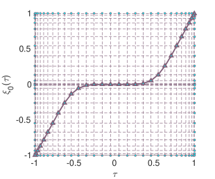
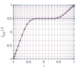
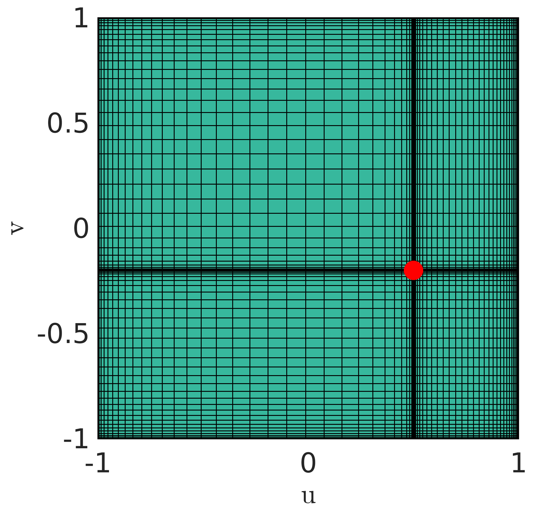
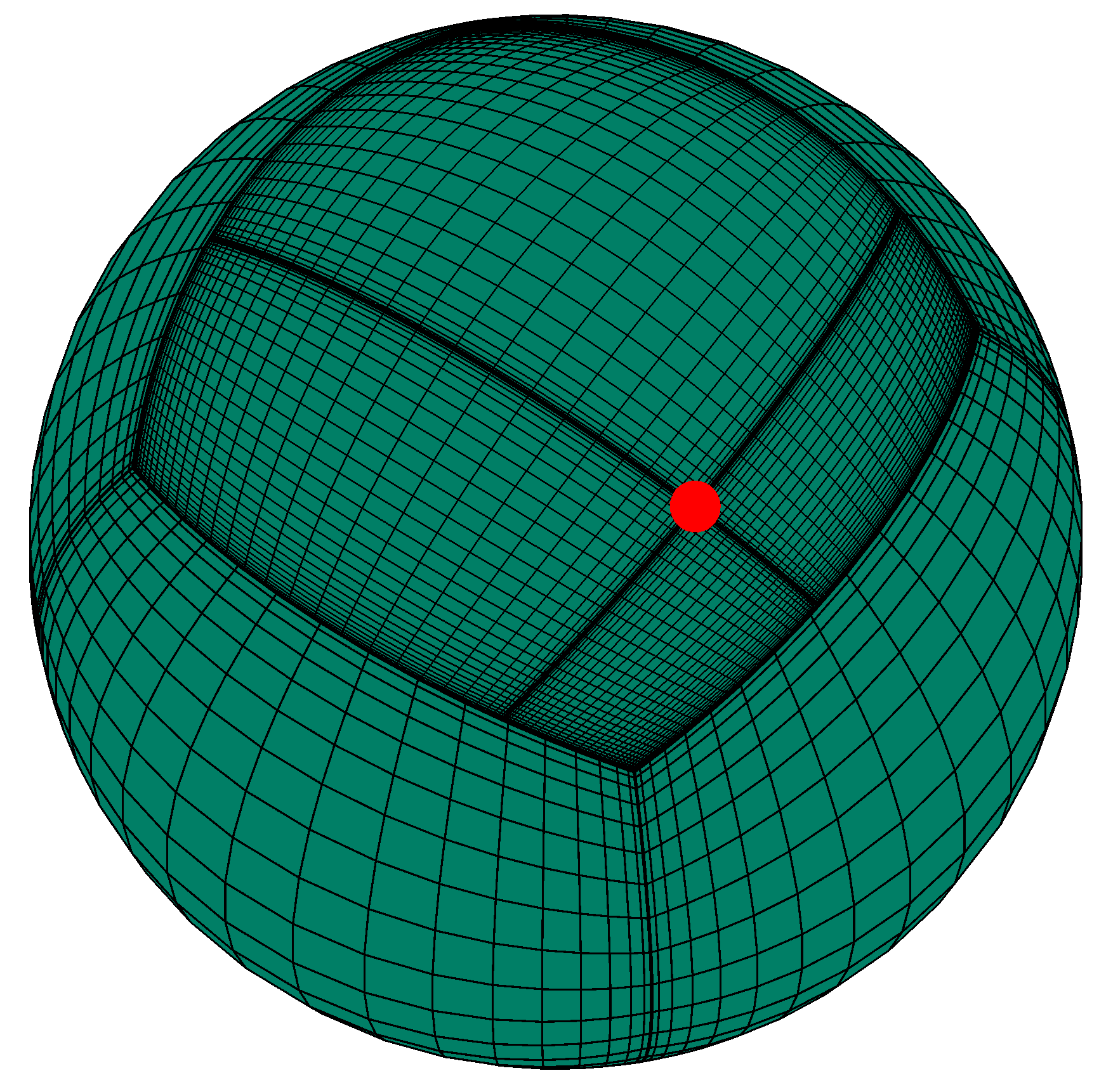
Figure 2: Top: Changes of variables (equation (40)) used to resolve the kernel singularity for two different values of $\alpha$. Bottom: Mesh (in both parameter space [left] and real space [right]) produced by the rectangular-polar change of variables to resolve the kernel singularity located at the point marked in red.

3.4 Computational cost

Let us now estimate the computational cost for the proposed method, focusing on the singular and near-singular integrals, as the cost of the non-adjacent interactions arises trivially from a double sum, and can be accelerated by means of either an equivalent source scheme [5, 6] or by a fast multipole (FMM) approach [14].

For the purposes of our computing-time estimates, let $N$ denote the maximum of the one dimensional discretization sizes ${N_{u}^{\,q}}$ and ${N_{v}^{\,q}}$ over all patches ($1\leq q\leq M$), and let $N^{\prime}_{\text{close}}$ denote the maximum, over all the patches, of the numbers of points that are close to the patch (they lie in $\Omega^{c}_{q}$), but which are not contained in the $q$-th patch. Additionally, let $N_{\beta}^{u}=N_{\beta}^{v}=N_{\beta}$ denote the number of quadrature points used for singular precomputations. With these notations we obtain the following estimates in terms of the bounded integer values $N$ (in the range of one to a few tens); the (large, proportional to the square of the frequency, for large frequencies) number $M$ of patches, and the related bounded parameters $N_{\beta}$ (of the order of one to a few hundreds):

• Cost of precomputations: $\mathcal{O}(MN_{\beta}^{2}(N^{2}+N^{\prime}_{\text{close}}))$ operations.

• Cost of forward map:

  • Chebyshev transform (partial summation): $\mathcal{O}(MN^{3})$.

  • Singular and near-singular interactions: $\mathcal{O}(MN^{2}(N^{2}+N^{\prime}_{\text{close}}))$.

  • Non-adjacent interactions $\mathcal{O}((M-1)^{2}N^{4})$ (or $M^{\alpha}N^{4}$ with $\alpha$ significantly smaller than two if adequate acceleration algorithms are utilized).

3.5 Patch splitting for large problems

Each patch requires creation and storage of a set of self-interaction weights $\beta_{n,m}^{\,q,\ell}$, for $q=1,\dots,M$, $n=1,\dots,N$, $m=1,\dots,N$ and $\ell=1,\dots,N^{2}$, at a total storage cost of $\mathcal{O}(MN^{4})$ double-precision complex-valued numbers. Additionally, weights also need to be stored for the $N^{\prime}_{\text{close}}$ near-singular points for each patch, and are dependent on the target point, then the total storage for the singular and near-singular weights is $\mathcal{O}(MN^{4}+MN^{2}N^{\prime}_{\text{close}})$.

In order to eliminate the need to evaluate and store a large number of weights that result as $N$ is increased, it is possible to instead increase the number of patches $M$—which causes the necessary number of weights to grow only linearly. In these regards it is useful to consider the following rule of thumb: in practice, as soon as the wavelength is accurately resolved by the single-patch algorithm, due to the spectral accuracy of Fejér’s first quadrature, only a few additional points per patch are needed to produce accuracies of the order of several digits. In view of the estimates in this and the previous section, parameter selections can easily be made by seeking to optimize the overall computing time given the desired accuracy and available memory.

4 Numerical results

This section presents a variety of numerical examples demonstrating the effectiveness of the proposed methodology. The particular implementation for the numerical experiments was programmed in Fortran and parallelized using OpenMP. The runs were performed on a single node of a dual socket Dell R420 with two Intel Xenon E5-2670 v3 2.3 GHz, 128GB of RAM. Unless otherwise stated, all runs where performed using 24 cores.

4.1 Forward map convergence

The accuracy of the overall solver depends crucially on the accuracy of the forward map computation. In this section we verify that the proposed methodology yields uniformly accurate evaluations of the action of the integral operator throughout the surface of the scatterer. To do so, we consider the eigenfunctions and eigenvalues of the single- and double-layer operators for Helmholtz equation [18, Sec. 3.2.3]:

$$S[Y_{\ell}^{m}(\theta,\varphi)] =kj_{\ell}(k)h_{\ell}^{(1)}(k)Y_{\ell}^{m}(\theta,\varphi),$$ (46)

$$\displaystyle D[Y_{\ell}^{m}(\theta,\varphi)] =\frac{k^{2}}{2}\left[j_{\ell}(k)\frac{\text{d}}{\text{d}k}h_{\ell}^{(1)}(k)+h_{\ell}^{(1)}\frac{\text{d}}{\text{d}k}j_{\ell}(k)\right]Y_{\ell}^{m}(\theta,\varphi),$$ (47)

where $j_{\ell}(k)$ and $h_{\ell}^{(1)}(k)$ are the spherical Bessel function of the first kind and spherical Hankel function respectively, and where $Y_{\ell}^{m}(\theta,\varphi)$ are the spherical harmonics. (For the spherical Hankel function $h_{\ell}^{(1)}(z)$ we have used the convention in [18]: $h_{\ell}^{(1)}(z)=-y_{\ell}(z)+i\;j_{\ell}(z)$, where $y_{\ell}$ is the $\ell$-th Neumann function.)

Figures 3 and 4 present convergence results for the combined field formulation we use, and in particular we demonstrate that the method is capable of obtaining accuracies close to machine precision (Figure 5).

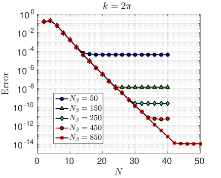
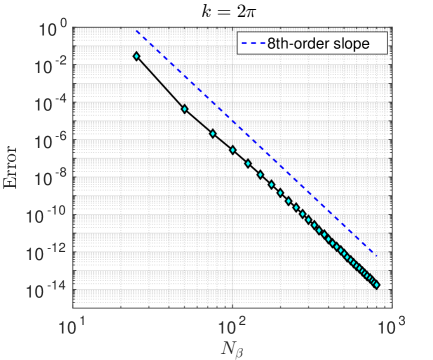
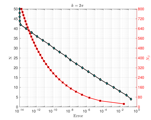
Figure 3: Convergence on the forward map of the combined field formulation for a unit sphere and wavenumber $k=2\pi$. Top-left: Error as we increase the number of points per patch (per dimension) for different values of $N_{\beta}$ used in the precomputations. Top-right: Error as a function of $N_{\beta}$. Bottom: Values of $N$ (black curve) and $N_{\beta}$ (red curve) for a given error.

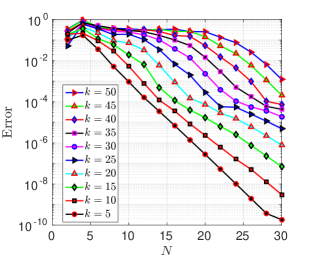
Figure 4: Error in the forward map of the combined field formulation for a unit sphere and for different wavenumbers as we increase the number of points per patch while keeping the numbers of patches fixed. A value of $N_{\beta}=250$ was used to guarantee that the error in the singular precomputations is not larger than the wavelength discretization error.

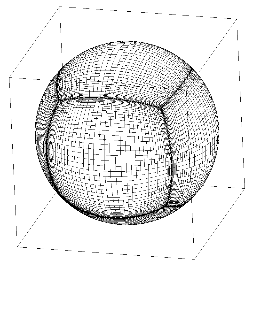
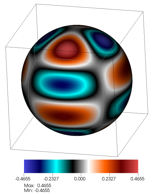
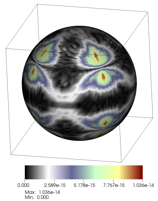
Figure 5: Mesh, forward map and pointwise error (from left to right) for a spherical harmonic density $(5,2)$ using a mesh of $N=50$ and $N_{\beta}=850$; the error is essentially uniform and accuracies close to machine precision are achieved.

As indicated in Section 3.5, for high-frequency problems it is beneficial to split the patches into smaller ones rather than increasing the numbers of points per patch, given that the storage only grows linearly as the number of patches is increased while keeping the number of points per patch constant. In order to determine the optimal balance between accuracy and efficiency, it must be considered that there are two factors that determine the accuracy of the method: (1) The order $N$ of the Chebyshev expansions used (i.e. the number of points per patch per dimension), and (2) The number of points per wavelength. Figure 6 displays the pointwise error in the forward map for a high frequency case, and Table 1 presents test results for several simple patch-splitting configurations, where the number of points per wavelength is calculated by the formula

$$\text{Points per }\lambda=\frac{N}{L/\lambda},$$ (48)

where $L^{2}={4\pi/M}$ is the average area of the quadrilateral patches for the sphere.

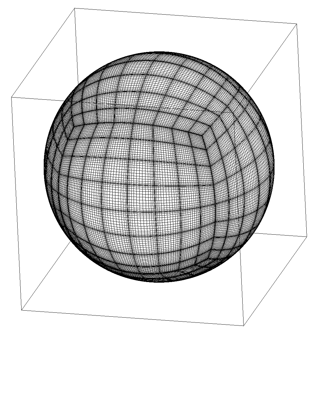
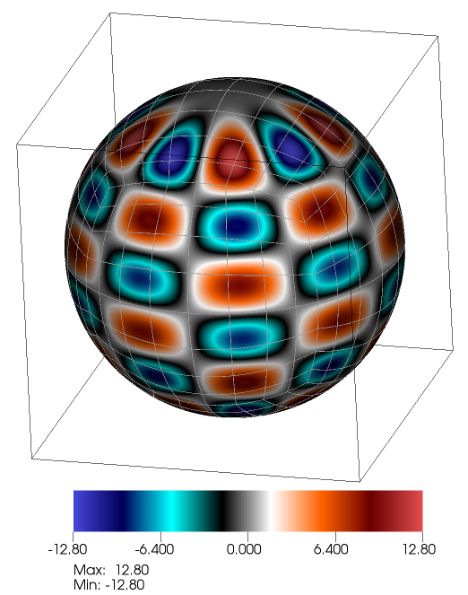
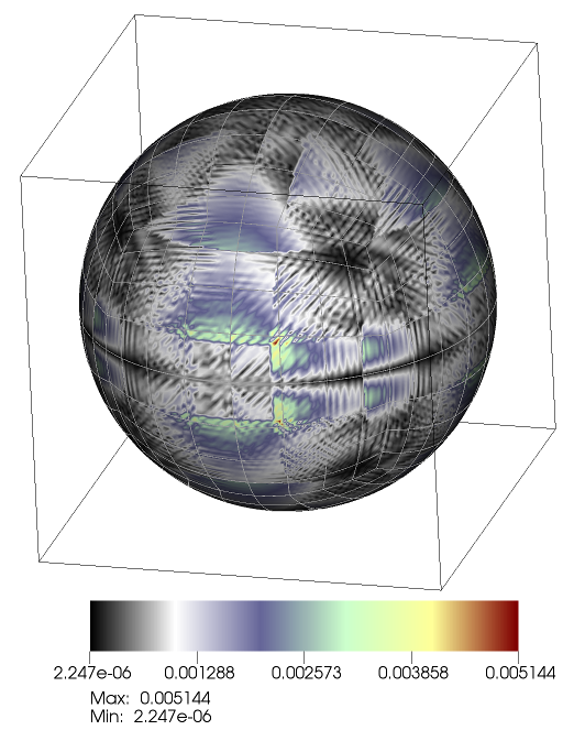
Figure 6: Mesh, forward map and pointwise error (from left to right) for a spherical harmonic density $(10,5)$. The figures show the patch splitting strategy for high frequencies. In this case $k=100$ which corresponds to scattering by a sphere $31.8\lambda$ in diameter, and and $6\times 8\times 8$ patches ($8\times 8$ subpatches in each one of $6$ initial patches) with $N=14$.

$N$	$N_{\beta}$	Patches	Points per $\lambda$	Unknowns	Time (prec.)	Time (1 iter.)	Error
$8$	$50$	$6\times 5\times 5$	$1.7$	$9600$	$1.39$ s	$0.18$ s	$71.3\%$
$12$	$60$	$6\times 5\times 5$	$2.6$	$21600$	$3.40$ s	$0.83$ s	$2.16\%$
$16$	$80$	$6\times 5\times 5$	$3.5$	$38400$	$9.26$ s	$2.41$ s	$0.0814\%$
$8$	$50$	$6\times 10\times 10$	$3.5$	$38400$	$16.74$ s	$2.78$ s	$0.336\%$
$12$	$70$	$6\times 10\times 10$	$5.2$	$86400$	$47.26$ s	$13.01$ s	$0.0238\%$
$16$	$90$	$6\times 10\times 10$	$6.9$	$153600$	$126.09$ s	$40.29$ s	$0.000355\%$

Table 1: Errors in the forward map (relative to the maximum forward map value) of the combined field operator for various patch splitting configurations and a spherical harmonic density (5,2). For the results in this table, $k=100$, a sphere of diameter $31.8\lambda$ was used, and all times reported for the precomputations and forward map where obtained using 24 computing cores. At this frequency, $N=16$ suffices to produce an accuracy of $0.08\%$ on the basis of six $5\times 5$ patches.

4.2 Edge geometries

As mentioned previously, the important problem of scattering by obstacles containing edges and corners presents several difficulties, including density and kernel singularities at the edges. In Figure 7, we demonstrate the performance of the method for a cube geometry by computing the error in the far field with respect to a reference solution obtained by using a very fine discretization. Figure 8 shows the scattering solution by a cube of side $5\lambda$.

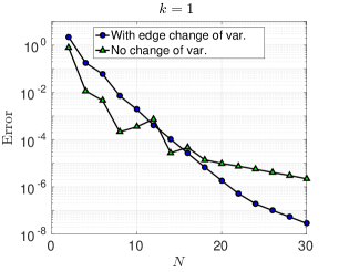
Figure 7: Maximum (absolute) far-field error for the problem of scattering by a cube of size $2\times 2\times 2$ and with $k=1$. The plot shows results excluding use of an edge change of variables (in green) and including an edge the change of variables with $p=2$ (in blue). The maximum value of the far field for the reference solution equals $2.144$.

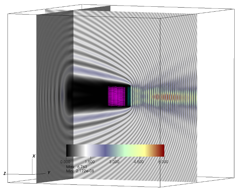
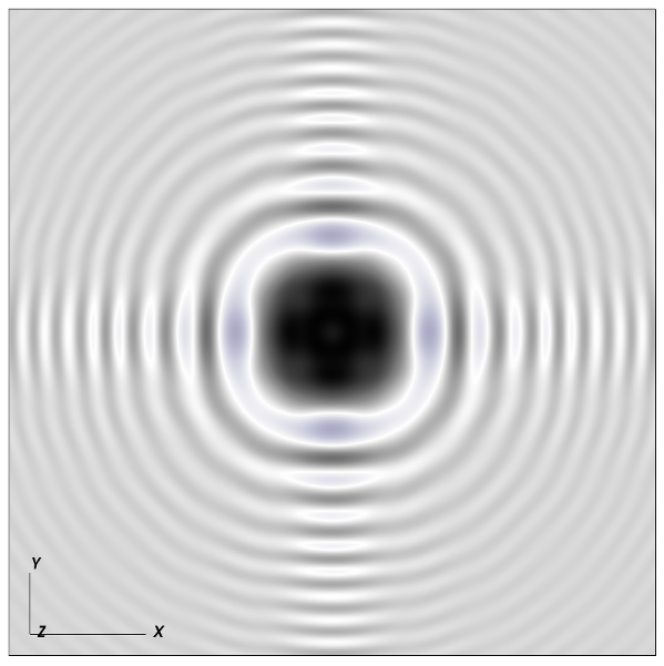
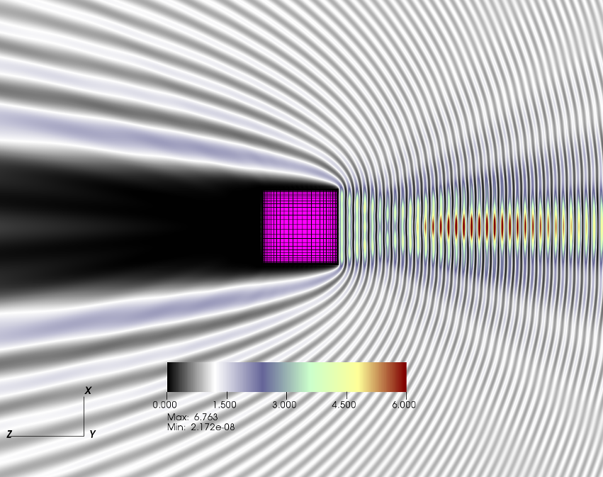
Figure 8: Scattering with $\lambda=0.4$ by a cube of size $2\times 2\times 2$ (each side of size $5\lambda$). The top-left image represents the real part of the total field and the other figures show the intensity ($|U|^{2}$) from different view angles.

4.3 Open surfaces

Methods for open surfaces typically suffer from low accuracies, or, alternatively, they require complex treatment at edges. The approach presented here is a straightforward application of the rectangular-polar method, with a change of variables at the edges, as described in Section 3.3. As demonstrated in Figure 9, which shows the convergence plot for the far field solution scattered by a disk, the method is robust and high-order accurate. Figure 10 shows the scattering solution for the problem of scattering by a disk $5\lambda$ in radius.

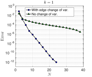
Figure 9: Maximum (absolute) far-field error for the problem of scattering by a disk of radius 1 and $k=1$. The plot shows both the curve excluding changes of variables (in green) and including a $p=4$ change of variables (in blue). The maximum value of the far field for the reference solution equals $0.7284$.

4.4 CAD geometries

As indicated in Section 2.3, as a rule, CAD designs can easily be re-expressed as a union of logically-quadrilateral explicitly parametrized patches, and they are thus particularly well-suited for use in conjunction with the proposed rectangular-polar solver. To demonstrate the applicability of the solver to such general type of geometry descriptions, Figure 11 presents the solution to the problem of acoustic scattering by a glider CAD design consisting of 87 patches.

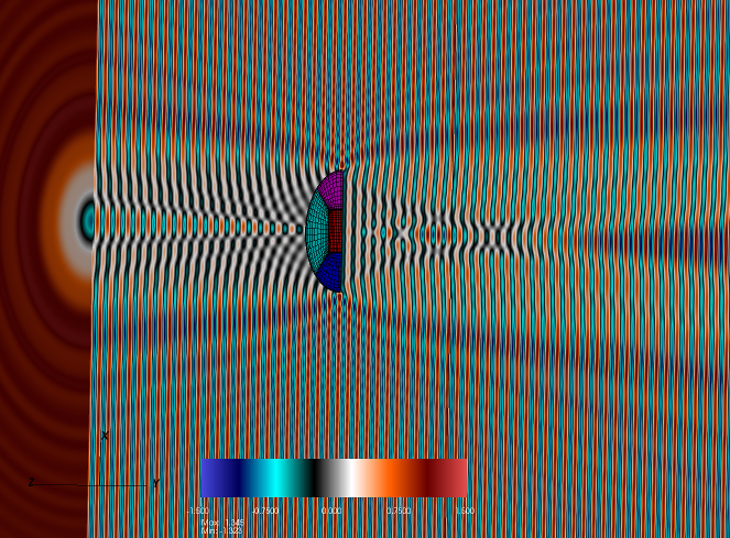
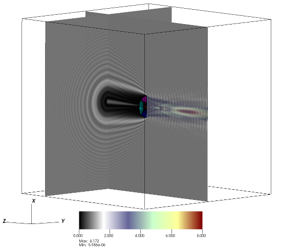
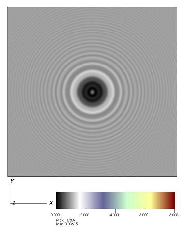
Figure 10: Scattering by a radius-one disk illuminated by a plane wave in the $+z$ direction (normal incidence), with $k=10\pi$ ($\lambda=0.2$). The image at the top-left displays the real value of the total field, while the other images depict the intensity ($|U|^{2}$) at different view angles. The solution presents the well-known Poisson spot (also known as Arago spot and Fresnel bright spot) generated at the center of the shaded region.

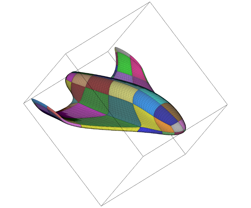
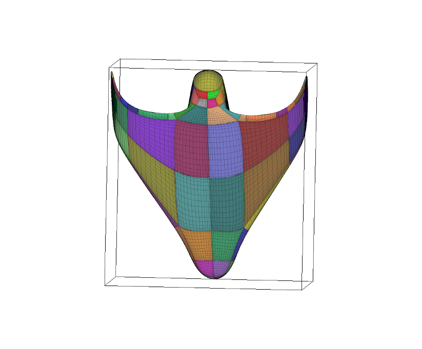
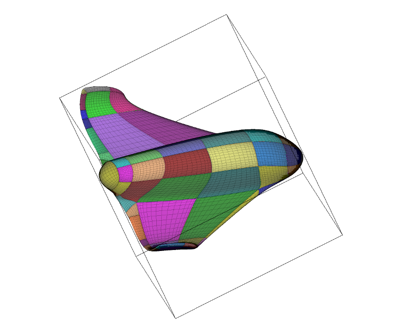
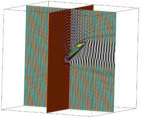
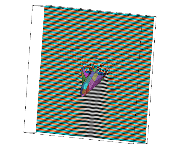
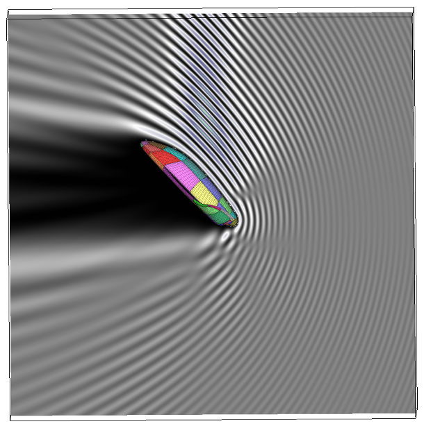
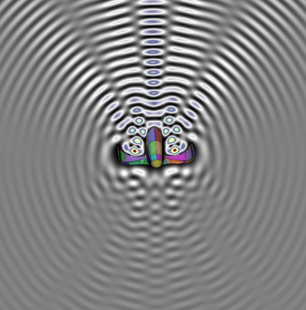
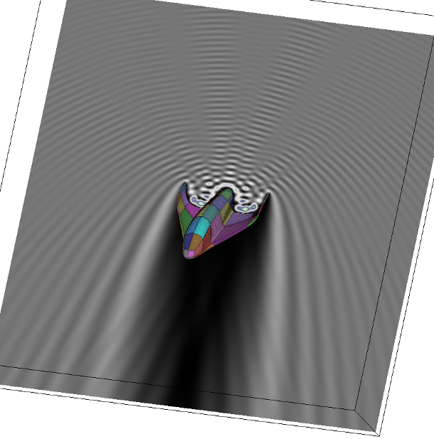
Figure 11: Acoustic scattering by a glider geometry from a CAD design. Top row: patches and mesh used. Mid row: Real part of the total field. Bottom row: Intensity of the total field ($|U|^{2}$).

5 Conclusions

We have presented a rectangular-polar integration strategy for singular kernels in the context of boundary integral equations. The methodology was then used in conjunction with the GMRES linear algebra solver to produce solutions of problems of scattering by obstacles consisting of open and closed surfaces. As demonstrated by a variety of examples presented in Section 4, the overall solver produces results with high-order accuracy, and the rectangular patch description of the geometry makes the algorithm particularly well-suited for application to engineering configurations—where the scattering objects are prescribed in standard (but generally highly complex) CAD representations.

The proposed methodology has been presented for the context of sound-soft acoustic scattering, but given the similar nature of the kernels appearing in the sound-hard case [3], the solver can also be used in that case. Preliminary results have shown that this solver is also suitable for electromagnetic scattering in both the perfect electric conductor (PEC) and dielectric cases. The numerical examples presented in this paper suggest that the proposed methodology affords a fast, accurate and versatile high-order integration and solution methodology for the problem of scattering by arbitrary engineering structures which, when combined with appropriate acceleration methods, should result in an accurate solver for highly complex, electrically or acoustically large problems of propagation and scattering.

References

- [1] J. P. Boyd. Chebyshev and Fourier Spectral Methods. Dover Publications, Inc., Mineola, New York, second edition, 2001.
- [2] J. Bremer and Z. Gimbutas. A Nyström method for weakly singular integral operators on surfaces. Journal of Computational Physics, 231(14):4885–4903, may 2012.
- [3] O. P. Bruno, T. Elling, and C. Turc. Regularized integral equations and fast high-order solvers for sound-hard acoustic scattering problems. International Journal for Numerical Methods in Engineering, 91:1045–1072, 2012.
- [4] O. P. Bruno, E. Garza, and C. Pérez-Arancibia. Windowed Green Function Method for Nonuniform Open-Waveguide Problems. IEEE Transactions on Antennas and Propagation, 65(9):4684–4692, sep 2017.
- [5] O. P. Bruno and L. A. Kunyansky. A Fast, High-Order Algorithm for the Solution of Surface Scattering Problems: Basic Implementation, Tests, and Applications. Journal of Computational Physics, 169(1):80–110, may 2001.
- [6] O. P. Bruno and L. A. Kunyansky. Surface scattering in three dimensions: an accelerated high-order solver. Proceedings of the Royal Society A: Mathematical, Physical and Engineering Sciences, 457:2921–2934, 2001.
- [7] O. P. Bruno and S. K. Lintner. A high-order integral solver for scalar problems of diffraction by screens and apertures in three-dimensional space. Journal of Computational Physics, 252:250–274, nov 2013.
- [8] O. P. Bruno, M. Lyon, C. Pérez-Arancibia, and C. Turc. Windowed Green Function Method for Layered-Media Scattering. SIAM Journal on Applied Mathematics, 76(5):1871–1898, jan 2016.
- [9] O. P. Bruno, J. S. Ovall, and C. Turc. A high-order integral algorithm for highly singular PDE solutions in Lipschitz domains. Computing, 84(3-4):149–181, 2009.
- [10] O. P. Bruno and C. Pérez-Arancibia. Windowed Green function method for the Helmholtz equation in the presence of multiply layered media. Proceedings of the Royal Society A: Mathematical, Physical and Engineering Science, 473(2202):20170161, jun 2017.
- [11] D. Colton and R. Kress. Inverse Acoustic and Electromagnetic Scattering Theory. Springer, New York, third edition, 2013.
- [12] M. Costabel and M. Dauge. General edge asymptotics of solutions of second-order elliptic boundary value problems I. Proceedings of the Royal Society of Edinburgh: Section A Mathematics, 123(01):109–155, nov 1993.
- [13] M. Ganesh and I. Graham. A high-order algorithm for obstacle scattering in three dimensions. Journal of Computational Physics, 198(1):211–242, jul 2004.
- [14] N. A. Gumerov and R. Duraiswami. Fast multipole methods for the Helmholtz equation in three dimensions. Elsevier, San Diego, first edition, 2004.
- [15] B. M. Johnston, P. R. Johnston, and D. Elliott. A sinh transformation for evaluating two-dimensional nearly singular boundary element integrals. International Journal for Numerical Methods in Engineering, 69(7):1460–1479, feb 2007.
- [16] P. R. Johnston and D. Elliott. A sinh transformation for evaluating nearly singular boundary element integrals. International Journal for Numerical Methods in Engineering, 62(4):564–578, jan 2005.
- [17] J. Markkanen, P. Ylä-Oijala, and A. Sihvola. Surface integral equation method for scattering by DB objects with sharp wedges. Applied Computational Electromagnetics Society Journal, 26(5):367–374, 2011.
- [18] J.-C. Nédélec. Acoustic and Electromagnetic Equations: Integral Representations for Harmonic Problems. Springer, New York, first edition, 2001.
- [19] C. Pérez-Arancibia. Windowed integral equation methods for problems of scattering by defects and obstacles in layered media. PhD thesis, California Institute of Technology, Applied and Computational Mathematics, Pasadena, CA, USA, 2016.
- [20] W. H. Press, S. A. Teukolsky, W. T. Vetterling, and B. P. Flannery. Numerical recipes: the art of scientific computing. Cambridge University Press, New York, third edition, 2007.
- [21] J. Waldvogel. Fast Construction of the Fejér and Clenshaw-Curtis Quadrature Rules. BIT Numerical Mathematics, 46(1):195–202, mar 2006.