Symmetry Enforced Chiral Hinge States and Surface Quantum Anomalous Hall Effect in Magnetic Axion Insulator $\text{Bi}_{2-x}\text{Sm}_{x}\text{Se}_{3}$

Abstract

A universal mechanism to generate chiral hinge states in the ferromagnetic axion insulator phase is proposed, which leads to an exotic transport phenomena, the quantum anomalous Hall effect (QAHE) on some particular surfaces determined by both the crystalline symmetry and the magnetization direction. A realistic material system Sm doped $\text{Bi}_{2}\text{Se}_{3}$ is then proposed to realize such exotic hinge states by combing the first principle calculations and the Green’s function techniques. A physically accessible way to manipulate the surface QAHE is also proposed, which makes it very different from the QAHE in ordinary 2D systems.

The bulk-boundary correspondence Ryu and Hatsugai (2002) is one of the most important physical consequences of the topological matter. In most of the cases, the bulk-boundary correspondence refers to the existing of guaranteed gapless quasi-particle excitations on the ($d-1$)-dimensional boundary (with $d$ being the dimension of the system), given that the symmetries required to protect such a topological state are still preserved on the boundary Hatsugai (1993); Kane and Mele (2005); Fu (2011); Hsieh et al. (2012); Wang et al. (2016). Very recently a new type of bulk-boundary correspondence was proposed for a special class of topological materials called second order topological insulators (SOTIs) Benalcazar et al. (2017a); Langbehn et al. (2017); Ezawa (2018); Schindler et al. (2017); Song et al. (2017); Fang and Fu (2017); Benalcazar et al. (2017b); Schindler et al. (2018), where the corresponding topological quasi-particle states appear in the $(d-2)$ instead of $(d-1)$-dimensional boundaries. In particular, non-trivial corner states (0D) will appear at the corners of a two dimensional SOTI and helical/chiral hinge states (1D) will appear at some particular hinges of a three dimensional SOTI.

Similar to the ordinary TI Kane and Mele (2005); Hasan and Kane (2010); Qi and Zhang (2011); Ando and Fu (2015), the general definition of SOTI can be expressed as the band insulators that can not be smoothly deformed to the atomic insulators Soluyanov and Vanderbilt (2011); Po et al. (2017); Bradlyn et al. (2017) without symmetry breaking or closing the bulk energy gap. Unlike topological insulators where each surface is gapless, a generic ($d-1$)-dimensional surface of $d$-dimensional SOTI is gapped, but on the entire boundary of a sample, there must be ($d-2$)-dimensional domain walls between surfaces having opposite masses, at which are located gapless topological modes. For the 2D SOTI, additional chiral or charge conjugation symmetry is required to protect the corner states Langbehn et al. (2017), which is difficult to realize in materials. While for 3D SOTI, the chiral or helical hinge states can be enforced by some bulk crystalline topological invariants, i.e. the mirror Chern number (MCN) $C_{m}$, but protected by more general symmetriesSong et al. (2017); Fang and Fu (2017). For example, for the helical hinge states, as first introduced in Ref. Hsieh et al. (2012); Schindler et al. (2017), the existence of non-trivial hinge states can be enforced by the non-zero mirror Chern number $C_{m}=2N$ defined on some particular mirror invariant planes with $N$ being an odd integer. The non-trivial helical states will persist even when the mirror symmetry is no longer present and hence MCN cannot be defined. As long as both the bulk and surfaces around that particular hinge are all fully gapped, the only symmetry requirement to protect the non-trivial helical mode in such cases is the time reversal symmetry. In Ref. Schindler et al. (2017), SnTe with strain along the (100) direction is proposed to be the first realistic material which supports the non-trivial helical states on the hinge formed between (100) and (010) surfaces.

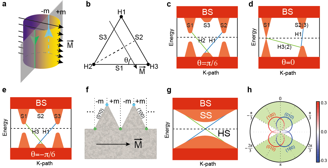
Figure 1: Schematic demonstration of the emergence of hinge states. (a) Chiral hinge states emerges on the domain wall of the surface states with magnetic polarization applied perpendicular to the mirror plane. (b) 3-D TI with $C_{3v}$ symmetry, and (c) to (e) schematically illustrate the evolution of its surface states and hinge states with the magnetic polarization applied along different directions. (f) The proposed configuration of the magnetically doped $\text{Bi}_{2}\text{Se}_{3}$ sample that can be adopted to detect the chiral hinge states. (g) The schematic plot of the energy dispersion of the corresponding hinge states in (f). (h)The ratio $m/|\vec{\text{M}}|$ for (010) and (100) surface states as a function of the direction of magnetization, $\theta$. The green shaded area labels the range of $\theta$ where hinges state are formed. For (a) and (c) to (g), blue and green lines denote two hinge states with opposite chirality.

Compared to helical hinge states, chiral hinge states are even more stable, which requires no symmetry to protect them. Similar to the chiral edge states in the 2D quantum Hall systems Klitzing et al. (1980); Hatsugai (1993), the chiral hinge states associated with a specific surface will lead to surface quantum anomalous Hall effect (QAHE) Mong et al. (2010); Nomura and Nagaosa (2011), which is the QAHE Haldane (1988); Yu et al. (2010); Chang et al. (2013) on a completely three dimensional object and has never been observed in any condensed matter systems before. In the present letter, we will propose that both the chiral hinge states and hence the surface QAHE can be realized in ferromagnetic axion insulators. After that we further propose a realistic material system, Sm doped $\text{Bi}_{2}\text{Se}_{3}$ single crystal, to realize such an axion insulator and SOTI with chiral hinge states. The high quality single crystal of Sm doped $\text{Bi}_{2}\text{Se}_{3}$ has been already obtained in Ref. Chen et al. (2015) with very low carrier density and Curie temperature as high as 52K. The easy axis of the magnetization has been confirmed experimentally to be within the $ab$ plane. From our DFT calculations, the effective exchange field acting on the low-energy bands is around 20 meV, which is much smaller than the semiconductor gap in $\text{Bi}_{2}\text{Se}_{3}$, thus keeping the system within the axion insulator phase. The presence of the chiral hinge states can be illustrated schematically in Fig. 1(b). Since the crystal structure of $\text{Bi}_{2}\text{Se}_{3}$ contains three vertical mirror planes, one of them can survive the ferromagnetic order by putting the magnetization direction perpendicular to that mirror plane as shown in Fig. 1(b). The original Dirac surface states on different sides of the mirror plane (S1 and S3) will acquire finite masses, which have opposite signs forced by the mirror symmetry as illustrated in Fig. 1(b). Therefore on hinge H2 between surface S1 and S3 in Fig. 1 (b), a domain wall between massive Dirac surface states with different mass signs is enforced by the mirror symmetry, leading to 1D chiral states on the corresponding hinge. Since the 1D chiral mode is stable against any weak perturbations, when the Zeeman field rotates away from the symmetric position and the system no longer has a mirror symmetry, the chiral hinge states cannot disappear immediately. However its location can be modified or even moved from one hinge to another once the gap on surface S1 or S3 is closed and reopen, as illustrated schematically in Fig.  1 (c) to (e).

The above argument can be made more general. In quantum electrodynamics, Lorentz invariance allows, in addition to the Maxwell term, a topological term of the form $\frac{\theta}{4\pi}\mathbf{E}\cdot\mathbf{B}$, where the coupling strength $\theta$ is called the axion fieldWilczek (1987). A static $\theta$ is quantized to $0$ or $\pi$ in the presence of time-reversal symmetry Qi et al. (2008), and $\theta=0$ and $\pi$ for trivial and topological insulators respectively. It was then realized that in the absence of time-reversal, spatial symmetries can also quantize the value of $\theta$, inducing a natural generalization of topological insulatorsEssin et al. (2009). In fact, as long as the spatial symmetry is improper, i.e. it flips the orientation of the space, a uniform $\theta$ can only take $0$ or $\pi$. It is usually thought that at the boundary of a region with $\theta=\pi$, there are gapless 2D surface states, which are nothing but the single Dirac fermion in the case of topological insulators. However, if the symmetry quantizing $\theta$ is a spatial symmetry, which is the case for the FM axion insulators, the 2D surface states only exist if the interface preserves the symmetry, and on a surface where it is broken, a mass gap generically exists. This leads to another interesting possibility: the mass is enforced to change signs on the entire boundary of the topological state, creating domain walls of mass gapsZhang et al. (2013), because either the mirror reflection or the inversion symmetry flips the sign of the mass terms for the surface Dirac Hamiltonian. Along any one of these domain walls, there are 1D chiral modes, i.e. the $(d-2)$-dimensional topological edge states, the recently discovered boundary manifestation of the nontrivial topology in the bulk in the absence of gapless surface states. In Fig. 1(a), we illustrate the 1D chiral modes on the surface of 3D axion insulators protected by the improper symmetry, mirror reflection in this case.

To calculate the hinges states, we adopt an approximation where the low-energy physics of Sm doped $\text{Bi}_{2}\text{Se}_{3}$ can be modeled by the tight binding Hamiltonian for the pure $\text{Bi}_{2}\text{Se}_{3}$ together with a magnetic exchange field acting on the p-orbitals of both the Bi and Se atoms. Moreover, we generalize the recursive Green’s function methodSancho et al. (1985), which is widely used for the spectral functions of the surface or interface states, to calculate the hinge states for the SOTI (details given in appendix B). As shown in Fig. 2(c), two hinges (labeled as Left and Right respectively) are generated by joining two semi-infinite slabs along different directions, namely $[1,0,0]$ and $[0,1,0]$. The hinge area can then be viewed as the left and right ends of the interface region between the two slabs oriented along different directions, with the cross section perpendicular to the c-axis. The projected spectral functions for the two hinge regions can then be obtained following the standard procedures of the recursive Green’s function method Sancho et al. (1985).

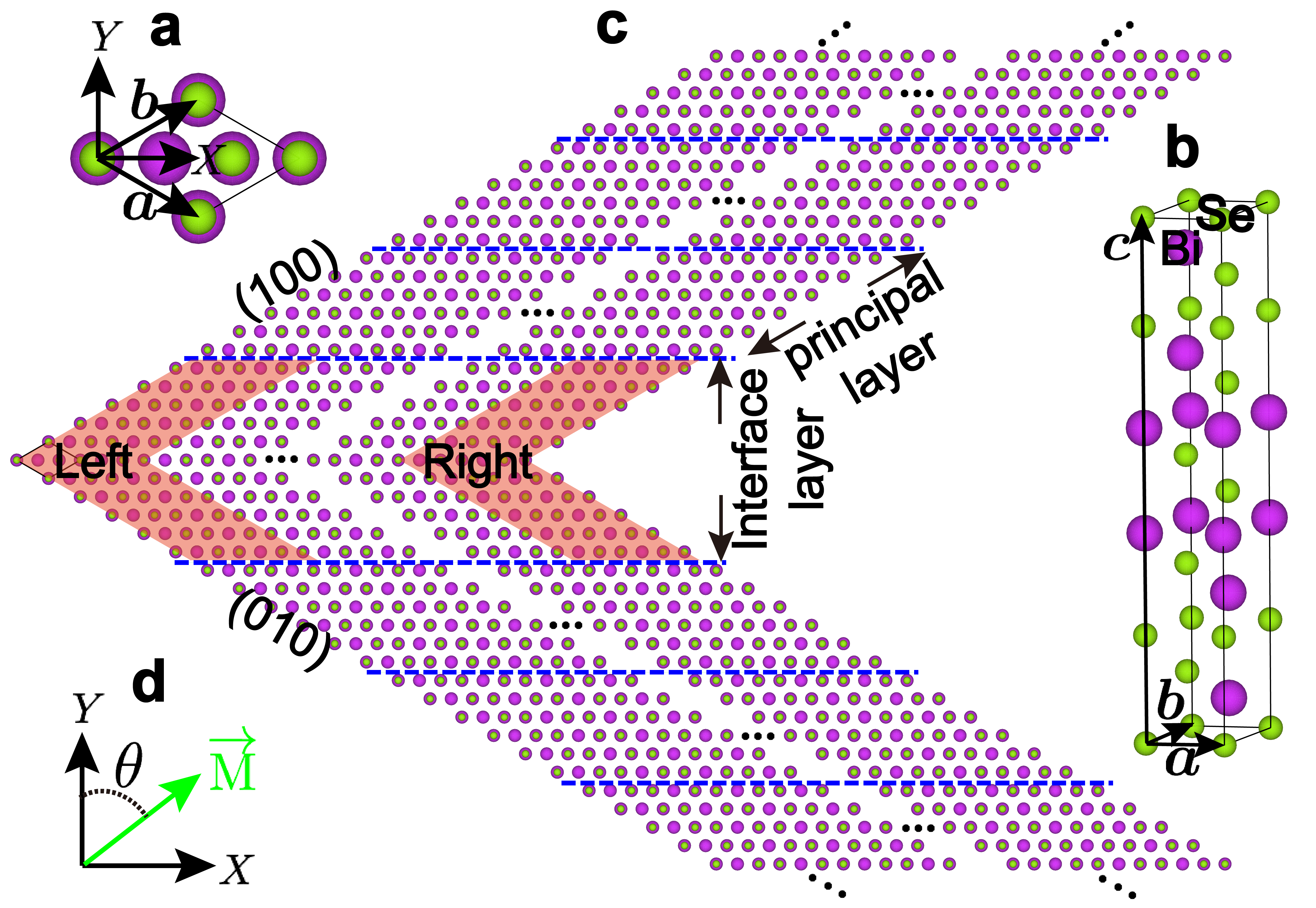
Figure 2: The structure proposed for the calculation of hinge states. (a), (b) Crystal structure of $\text{Bi}_{2}\text{Se}_{3}$. $X$, $Y$ and $Z$ form the global right-handed coordinate system. (c) The bi-semi-infinite open boundary geometry in which the (010) and (100) surfaces meet at left and right hinges parallel to $\boldsymbol{c}$ direction. The structure is semi-infinite along $\boldsymbol{a}$ and $\boldsymbol{b}$ direction, periodic along $\boldsymbol{c}$ direction, finite along $X$ direction. The length in $X$ direction is $20$ lattice constants. Principal layer (PL) is a group of atomic layers that is large enough such that only adjacent PLs interact. Interface layer is a group of atomic layers to connect two semi-infinite parts. Generally, interface layer is composed of the first PL along $\boldsymbol{a}$ direction combined with the first PL along $\boldsymbol{b}$ direction. (d) The easy direction of the magnetization $\boldsymbol{M}$ lies in the $ab$ plane, with $\theta$ the angle between $\boldsymbol{M}$ and $y$ axis.

As already confirmed experimentally Chen et al. (2015), in $\text{Sm}_{x}\text{Bi}_{2-x}\text{Se}_{3}$ the magnetic moments on Sm ions ordered ferromagnetically under $T_{c}\approx 52$K. The easy axis lies within the $ab$ plane and can be easily tuned by a small external magnetic field. The crystal structure of $\text{Bi}_{2}\text{Se}_{3}$ contains three vertical mirror planes and will survive the ferromagnetic order if the magnetization $M$ is along the $[-1,1,0]$, $[0,-1,0]$ and $[1,0,0]$ directions respectively, (corresponding to $\theta=0,2\pi/3$ and $4\pi/3$ in Fig. 1(b) respectively). Then as we discussed above, the existence of the mirror symmetry in the axion insulator will force the mass terms on the different sides of the mirror symmetric hinge to be opposite in sign, which guarantees the existence of the chiral hinge states centered at that particular hinge. Interestingly, since the chiral hinge states are topologically stable, the breaking of the corresponding mirror symmetry, i.e. by rotating the magnetization $M$ away from the particular angle mentioned above, the chiral hinge states won’t disappear immediately. In fact it will disappear only when the surface gap closes on either of the two nearby surfaces. Otherwise, as long as the gap still exists on both surfaces near the hinge, the domain wall feature still remains and the only effect of the mirror symmetry breaking is to modify the wave function of the hinge state to be asymmetric about the mirror plane.

The local spectral functions at both the left and right hinges can be obtained by projecting the imaginary part of the Green’s function to the corresponding hinge area, which can be expressed as $\rho_{L/R}(k_{z},\omega)={-1\over\pi}\sum_{i\in L/R}\text{Im}G_{ii}(k_{z},\omega)$, where the hinge area $L$ and $R$ are illustrated by the orange color shaded block Left and Right in Fig. 2(c), respectively. Then the hinge spectral functions can be obtained by applying the recursive Green’s function method introduced above. Alternatively the existence of chiral hinge modes can be inferred from checking the mass terms on the nearby surfaces, whose Hamiltonian can be written as

$$H_{SF}={\vec{v}}_{x}\cdot{\vec{\sigma}}k_{x}+{\vec{v}}_{y}\cdot{\vec{\sigma}}k_{y}+{\vec{g}}_{x}\cdot{\vec{\sigma}}M_{x}+{\vec{g}}_{y}\cdot{\vec{\sigma}}M_{y}+{\vec{g}}_{z}\cdot{\vec{\sigma}}M_{z},$$ (1)

where $x$, $y$, $z$ form the local right handed coordinate system and ${\vec{v}}_{i}$, ${\vec{g}}_{i}$ are vectors defined in pseudo-spin space. Both the velocity and g-factor vectors for the (100) and (010) surfaces of Sm_xBi_2-xSe₃ can be obtained by the corresponding surface calculations based on the effective tight binding Hamiltonian with their values listed in Table. 1.

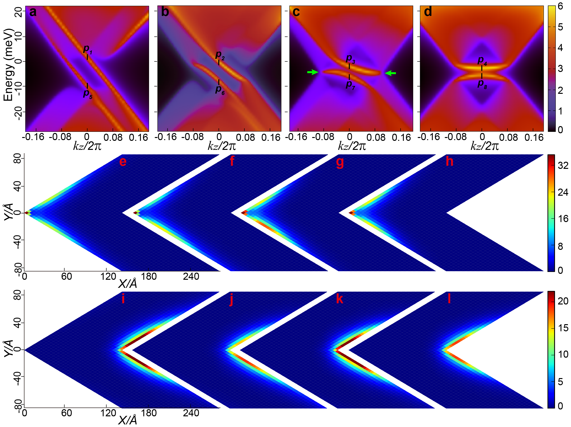
Figure 3: The projected spectral function (a-d) on the interface layer and their spatial distributions (e-l). From (a) to (d), $\boldsymbol{M}$ is rotated from $\theta=0$ to $\theta=\pi/6$, $\theta=\pi/3$ and $\theta=\pi/2$, respectively. Points $\{p_{1},\cdots,p_{8}\}$, with $k_{z}=0$, are labelled to show spatial distribution of these points in (e) to (l). From (e) to (h), we plot spatial distribution of spectral functions at $p_{1}$ to $p_{4}$ labelled in (a) to (d), showing spatially localized states distributed around the left hinge. From (i) to (l), we plot spatial distribution of spectral functions at $p_{5}$ to $p_{8}$ labelled in (a) to (d), showing spatially localized states distributed around the right hinge.

Table 1: Local right-handed coordinate system ${\boldsymbol{e}_{x,y,z}}$, velocity $v$ and g-factor $g$ of (010) and (100) surfaces, respectively. Entries of local $\boldsymbol{e}_{x,y,z}$ are given in terms of unit vectors of global coordinate system $x,y,z$ shown in Fig. 2-(a). Unit of $v$ is eV$\cdot\AA$ while unit of $g$ is 1/eV.

	(010)			(100)
$\boldsymbol{e}_{x}$	$\frac{\sqrt{3}}{2}$	$-\frac{1}{2}$	0	$-\frac{\sqrt{3}}{2}$	$-\frac{1}{2}$	0
$\boldsymbol{e}_{y}$	0	0	1	0	0	1
$\boldsymbol{e}_{z}$	$-\frac{1}{2}$	$-\frac{\sqrt{3}}{2}$	0	$-\frac{1}{2}$	$\frac{\sqrt{3}}{2}$	0
$\vec{v}_{x}$	0	0.4316	0.4951	0	0.4316	0.4951
$\vec{v}_{y}$	-0.7649	0	0	-0.7649	0	0
$\vec{g}_{x}$	0.7782	0	0	0.7782	0	0
$\vec{g}_{y}$	0	0.5354	-0.0957	0	0.5354	-0.0957
$\vec{g}_{z}$	0	0	0.4778	0	0	0.4778

Then the mass associated with that particular surface Dirac equation can be expressed as

$$m={{({\vec{v}}_{x}\times{\vec{v}}_{y})\cdot({\vec{g}_{x}}M_{x}+{\vec{g}_{y}}M_{y}+{\vec{g}_{z}}M_{z})}\over{|{\vec{v}}_{x}\times{\vec{v}}_{y}|}}.$$ (2)

Bearing in mind the fact that the magnetization lies in $ab$ plane and using velocity $v$ and g-factor $g$ listed in Table. 1, we can express $m$ as a function of magnetization direction $\theta$ as $m_{010}=-0.3140|\boldsymbol{M}|sin(\theta+\pi/3)$ and $m_{100}=-0.3410|\boldsymbol{M}|sin(\theta-\pi/3)$, which are plotted in Fig. 1(h).

The mass term vanishes at $\theta=\pi/3$ for the (100) surface and $\theta=2\pi/3$ for (010) indicating the surface topological transitions at these two angles, after which the hinge states moved from one hinge to another. As we discussed above, the chiral hinge states can only exist when the two nearby surfaces have the mass terms with opposite signs as indicated by the green area in Fig. 1(h).

In the first row of Fig. 3, we plot the hinge spectral functions calculated by the recursive Green’s function method for four typical magnetization direction, i.e. $0$, $\pi/6$, $\pi/3$ and $\pi/2$. In Fig. 3(a), the magnetization is along the $Y$ direction, which preserves the $XZ$ mirror plane. As we discussed above, the mirror symmetry guarantees the sign change for the mass terms on the nearby surfaces leading to chiral hinge states. The energy dispersion of the hinge states on both left and right hinges can be found by checking the spectral functions projected to the whole interface area, which are plotted in Fig. 3(a). Clear chiral hinge states can be found with a similar velocity around $-1.60\times 10^{5}m/s$. As shown in Fig. 3(e) and Fig. 3(i), the spacial distribution functions for the peaks marked as $p_{1}$ and $p_{5}$ in Fig. 3(a) are centered at the left and right hinges respectively, which are fully symmetric around the corresponding hinge due to the mirror symmetry. Further examination of the spatial distribution of the spectral weight confirms that the chiral hinge mode on each particular hinge smoothly connects the valence bands on the (100) surface and the conduction bands on the (010) surface. When the magnetization angle $\theta$ being rotated away clockwise from zero, the surface gap on (100) is getting smaller quickly and the hinge states are still there with slightly modified velocity and asymmetric spacial distribution around the hinge, as shown in Fig. 3(f). When the magnetization angle $\theta$ becomes $\pi\over 3$, the gap on (100) surface closes completely forming surface Dirac cones on the corresponding surfaces, as pointed by the two arrows in Fig. 3(c), which indicates the topological phase transition on these surfaces. After the transition the connection pattern of the hinge states changed completely, as shown in Fig. 3(d), the hinge states now connect within the conduction (label $p_{4}$) or the valence bands (label $p_{8}$) in (100) and (010) surfaces and become topologically trivial.

The existence of chiral hinge modes will cause quantum anomalous Hall effect on the surfaces of the $\text{Sm}_{x}\text{Bi}_{2-x}\text{Se}_{3}$. The experimental setup can be schematically plotted in Fig. 1(f). By cutting the $\text{Sm}_{x}\text{Bi}_{2-x}\text{Se}_{3}$ single crystal using the focused ion beam technique to obtain the zig-zag surface structure formed by (100) and (010) surfaces, the counter propagating chiral hinge modes can then be induced by the horizontal magnetization on the ”ridge” and ”valley” area as shown in Fig. 1(g). The surface Quantum anomalous Hall effect can be detected by standard four-lead measurement for the Hall effect.

In conclusion, we proposed in the paper that Sm doped Bi₂Se₃ single crystal is a magnetic axion insulator and provides an ideal material platform to realize helical hinge states on the particular hinges of the crystals. Such nontrivial hinge states demonstrate that the magnetic axion insulator can also be viewed as higher-order topological insulators with the new type of bulk-boundary correspondence described in the paper. The surface QAHE is the most striking observable effect caused by the chiral hinge states in Sm doped Bi₂Se₃ single crystal.

Appendix A Calculation of effective magnetic exchange field

Recently, Sm-doped $\text{Bi}_{2}\text{Se}_{3}$ magnetic topological insulators have been experimentally realized with the Curie temperature being about 52K Chen et al. (2015). We have simulated this system theoretically by the first principle method using VASP package Kresse and Hafner (1993); Kresse and FurthmÃŒller (1996); Kresse and Furthmüller (1996). In the calculation, a 2$\times$2$\times$1 supercell structure of $\text{Bi}_{2}\text{Se}_{3}$ is constructed with one Bi atom being replaced by a Sm atom. In such a $\text{SmBi}_{23}\text{Se}_{36}$ system, $\text{Sm}^{3+}$ is in the high-spin state and its total magnetization strength is as large as 5.4 $\mu_{B}$ . A very dense momentum and energy grid is adopted to calculate the spin polarized density of states of Bi and Se which are shown in Fig. A.1. The exchange field splitting $\Delta E$ of the $p$ orbitals can be roughly estimated by Eq.(A.1), which are about 20 meV and 10 meV for p-orbitals on Se and Bi respectively.

$$\Delta E=\frac{\int\epsilon\rho_{\downarrow}(\epsilon)d\epsilon}{\int\rho_{\downarrow}(\epsilon)d\epsilon}-\frac{\int\epsilon\rho_{\uparrow}(\epsilon)d\epsilon}{\int\rho_{\uparrow}(\epsilon)d\epsilon},$$ (A.1)

where $\rho_{\downarrow(\uparrow)}(\epsilon)$ is the density of state of the majority(minority) spin component of p orbitals.

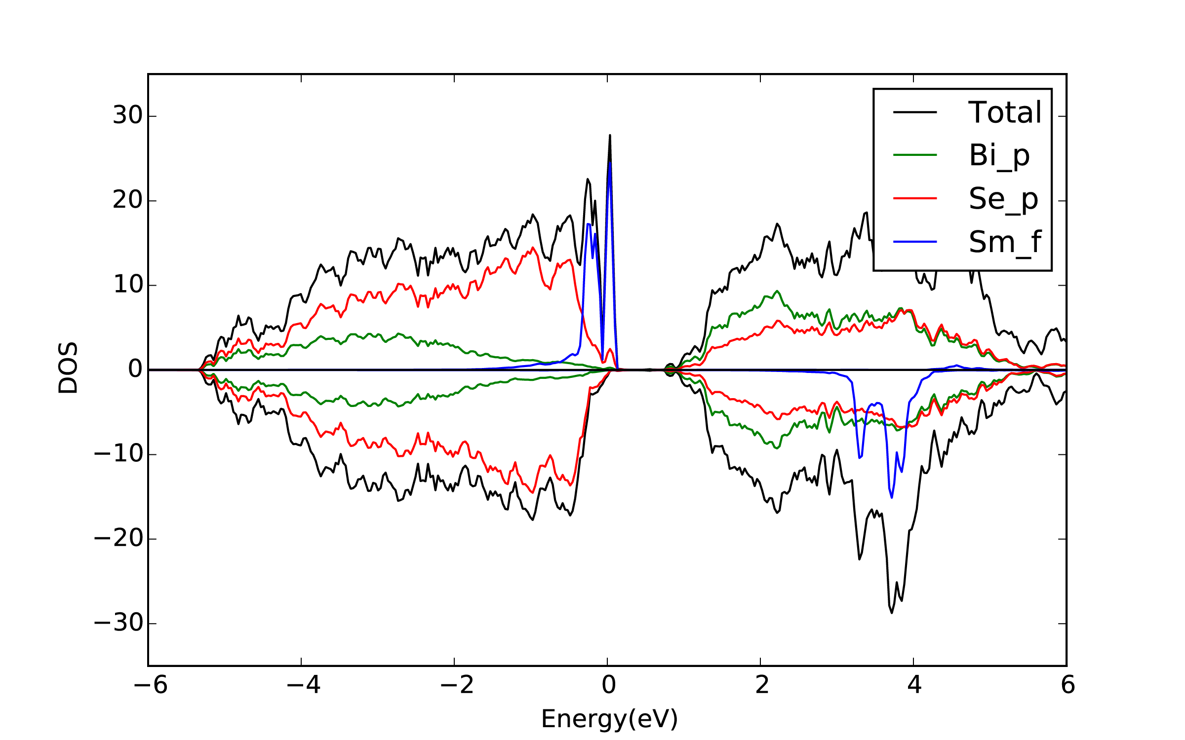
Figure A.1: Orbital-resolved density of states of $\text{SmBi}_{23}\text{Se}_{36}$ calculated by LDA method.

Appendix B Recursive Green Function method in calculation of hinge states

To carry out the realistic calculations for the hinge states, we design a bi-semi-infite open boundary geometry in which the (010) and (100) surfaces meet at left and right hinges parallel to $\boldsymbol{c}$ direction. The geometry is semi-infinite along $\boldsymbol{a}$ and $\boldsymbol{b}$ direction, periodic along $\boldsymbol{c}$ direction, finite along $x$ direction. The size along the $x$ direction is $20$ unit cells in realistic calculation ensuring negligible finite-size effects arising from hybridizations between left and right hinges. Principal layer (PL) is a group of atomic layers that is large enough such that only adjacent PLs interact. Division of ULs and LLs into principal layers is a common strategy to express the Hamiltonian into the block tridiagonal form,

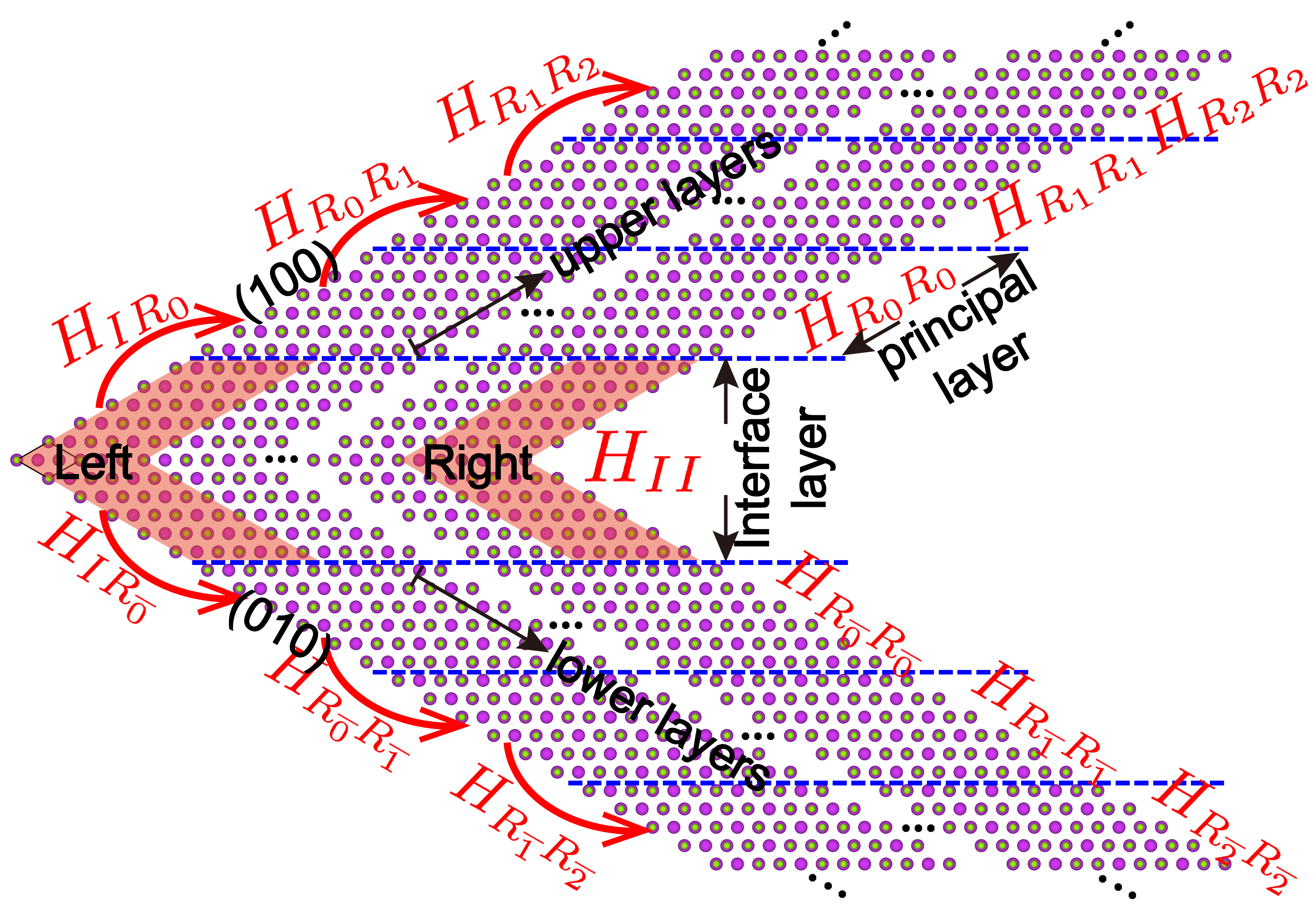
Figure B.1: The bi-semi-infinite open boundary geometry mentioned in the main text to calculate hinge states. The geometry is divided into three parts, interface layer, upper layers (ULs, divided into PLs which are positively labelled as $R_{i}$) and lower layers (LLs, divided into PLs which are negatively labelled as $R_{\overline{i}}$). Hamiltonian of each PL and interface layer as well as hopping matrix among them are given in this figure.

$$H=\left(\begin{array}[]{cccccccccc}H_{II}&H_{IR_{0}}&H_{IR_{\overline{0}}}&0&\cdots\\ H_{IR_{0}}^{\dagger}&H_{R_{0}R_{0}}&0&H_{R_{0}R_{1}}&0&\cdots\\ H_{IR_{\overline{0}}}^{\dagger}&0&H_{R_{\overline{0}}R_{\overline{0}}}&0&H_{R_{\overline{0}}R_{\overline{1}}}&0&\cdots\\ 0&H_{R_{0}R_{1}}^{\dagger}&0&H_{R_{1}R_{1}}&0&H_{R_{1}R_{2}}&0&\cdots\\ \vdots&0&H_{R_{\overline{0}}R_{\overline{1}}}^{\dagger}&0&H_{R_{\overline{1}}R_{\overline{1}}}&0&H_{R_{\overline{1}}R_{\overline{2}}}&0&\cdots\\ &\vdots&0&H_{R_{1}R_{2}}^{\dagger}&0&H_{R_{2}R_{2}}&0&H_{R_{2}R_{3}}&0&\cdots\\ &&\vdots&0&H_{R_{\overline{1}}R_{\overline{2}}}^{\dagger}&0&H_{R_{\overline{2}}R_{\overline{2}}}&0&H_{R_{\overline{2}}R_{\overline{3}}}&\ddots\\ &&&\vdots&\ddots&\ddots&\ddots&\ddots&\ddots&\ddots\\ \\ \\ \end{array}\right)$$ (B.1)

where the diagonal block $H_{R_{i}R_{i}}=H_{R_{0}R_{0}}$, $H_{R_{\overline{i}}R_{\overline{i}}}=H_{R_{\overline{0}}R_{\overline{0}}}$ and the hopping matrix $H_{R_{i}R_{i+1}}=H_{R_{0}R_{1}}$, $H_{R_{\overline{i}}R_{\overline{i+1}}}=H_{R_{\overline{0}}R_{\overline{1}}}$ Implicitly, each block of $H$ is a function of momentum $k_{z}$, i.e. $H_{\cdot\cdot}\equiv H_{\cdot\cdot}(k_{z})$. The tight binding Hamiltonian is obtained from the maximally-localized Wannier functions constructed by wannier90 Mostofi et al. (2014) package interfaced to VASP Kresse and Hafner (1993); Kresse and FurthmÃŒller (1996); Kresse and Furthmüller (1996). Furthermore, Zeeman terms $H_{z}=\boldsymbol{M}\cdot\boldsymbol{\sigma}$ with the strength obtained from the first principle calculations mentioned in the previous section are added to all $p$ orbitals to simulate the ferromagnetic order arising from Sm doping.

For simplification, $H_{IR}$ is used to denote hoppings between interface layer and ULs, LLs

$$H_{IR}\equiv\left(\begin{array}[]{cccc}H_{IR_{0}}&H_{IR_{\overline{0}}}&0&\cdots\end{array}\right).$$ (B.2)

$H_{P}$, in block tridiagonal form, is to denote Hamiltonian of ULs,

$$H_{P}\equiv\left(\begin{array}[]{ccccc}H_{R_{0}R_{0}}&H_{R_{0}R_{1}}&0\\ H_{R_{0}R_{0}}^{\dagger}&H_{R_{0}R_{0}}&H_{R_{0}R_{1}}&0\\ 0&H_{R_{0}R_{0}}^{\dagger}&H_{R_{0}R_{0}}&H_{R_{0}R_{1}}&\ddots\\ &\ddots&\ddots&\ddots&\ddots\\ \\ \end{array}\right),$$ (B.3)

and $H_{N}$ , also in block tridiagonal form, is to denote Hamiltonian of LLs

$$H_{N}\equiv\left(\begin{array}[]{ccccc}H_{R_{\overline{0}}R_{\overline{0}}}&H_{R_{\overline{0}}R_{\overline{1}}}&0\\ H_{R_{\overline{0}}R_{\overline{1}}}^{\dagger}&H_{R_{\overline{0}}R_{\overline{0}}}&H_{R_{\overline{0}}R_{\overline{1}}}&0\\ 0&H_{R_{\overline{0}}R_{\overline{1}}}^{\dagger}&H_{R_{\overline{0}}R_{\overline{0}}}&H_{R_{\overline{0}}R_{\overline{1}}}&\ddots\\ &\ddots&\ddots&\ddots&\ddots\\ \\ \end{array}\right).$$ (B.4)

Furthermore, we introduce a new “direct sum” operation $\tilde{\oplus}$ of two square matrix $A$ and $B$ as

$$A\tilde{\oplus}B=\left(\begin{array}[]{ccccc}A_{11}&0&A_{12}&0&\cdots\\ 0&B_{11}&0&B_{12}&\cdots\\ A_{21}&0&A_{22}&0&\cdots\\ 0&B_{21}&0&B_{22}&\cdots\\ \vdots&\vdots&\vdots&\vdots&\ddots\end{array}\right).$$ (B.5)

Now we have

$$H\equiv\left(\begin{array}[]{cc}H_{II}&H_{IR}\\ H_{IR}^{\dagger}&H_{RR}\end{array}\right),$$ (B.6)

where

$$H_{RR}\equiv H_{P}\tilde{\oplus}H_{N},$$ (B.7)

indicating that ULs and LLs are totally decoupled from each other.

The imaginary part of the interface Green function $G_{II}(k_{z},\omega)$ can be written as,

$$A_{II}(k_{z},\omega)=-\frac{1}{\pi}\Im G_{II}(k_{z},\omega),$$ (B.8)

$$G\equiv\left(\begin{array}[]{cc}G_{II}&G_{IR}\\ G_{IR}^{\dagger}&G_{RR}\end{array}\right),$$ (B.9)

$$(\omega+i\eta)G=1,$$ (B.10)

$$G_{II}(k_{z},\omega+i\eta)=\left[(\omega+i\eta)-H_{II}-\Sigma_{R}\right]^{-1},$$ (B.11)

where $\Sigma_{R}$ is the self-energy depicting comprehensive interactions between interface layer and ULs, LLs. Within the approximation of PL, $\Sigma_{R}$ has a simple form as

$$\Sigma_{R}=H_{IR}g_{RR}H_{IR}^{\dagger}\approx H_{IR_{0}}g_{R_{0}R_{0}}H_{IR_{0}}^{\dagger}+H_{IR_{\overline{0}}}g_{R_{\overline{0}}R_{\overline{0}}}H_{IR_{\overline{0}}}^{\dagger}$$ (B.12)

where $g_{R_{0}R_{0}}$ and $g_{R_{\overline{0}}R_{\overline{0}}}$ is the “surface” Green function of ULs and LLs, respectively. Because $H_{P}$ and $H_{N}$ are all in triangular diagonal form, $g_{R_{0}R_{0}}$ and $g_{R_{\overline{0}}R_{\overline{0}}}$ can be solved by the standard recursive schemes Sancho et al. (1985). Using equations (B.12, B.11, B.8), we obtain the spectral functions for the interface layer. $A_{II}$ is a square matrix with its indices being the number of orbitals in the interface layer. The trace of $A_{II}$ gives the integrated spectral shown in the first row of Fig. 3.

References

- Ryu and Hatsugai (2002) S. Ryu and Y. Hatsugai, Phys. Rev. Lett. 89, 077002 (2002).
- Hatsugai (1993) Y. Hatsugai, Phys. Rev. Lett. 71, 3697 (1993).
- Kane and Mele (2005) C. L. Kane and E. J. Mele, Phys. Rev. Lett. 95, 146802 (2005).
- Fu (2011) L. Fu, Phys. Rev. Lett. 106, 106802 (2011).
- Hsieh et al. (2012) T. H. Hsieh, H. Lin, J. Liu, W. Duan, A. Bansil, and L. Fu, Nature communications 3, 982 (2012).
- Wang et al. (2016) Z. Wang, A. Alexandradinata, R. J. Cava, and B. A. Bernevig, Nature 532, 189 (2016).
- Benalcazar et al. (2017a) W. A. Benalcazar, B. A. Bernevig, and T. L. Hughes, Phys. Rev. B 96, 245115 (2017a).
- Langbehn et al. (2017) J. Langbehn, Y. Peng, L. Trifunovic, F. von Oppen, and P. W. Brouwer, Phys. Rev. Lett. 119, 246401 (2017).
- Ezawa (2018) M. Ezawa, Phys. Rev. B 97, 155305 (2018).
- Schindler et al. (2017) F. Schindler, A. M. Cook, M. G. Vergniory, Z. Wang, S. S. P. Parkin, B. A. Bernevig, and T. Neupert, ArXiv e-prints (2017), arXiv:1708.03636 [cond-mat.mes-hall] .
- Song et al. (2017) Z. Song, Z. Fang, and C. Fang, Phys. Rev. Lett. 119, 246402 (2017).
- Fang and Fu (2017) C. Fang and L. Fu, arXiv:1709.01929 [cond-mat, physics:hep-th] (2017), arXiv: 1709.01929.
- Benalcazar et al. (2017b) W. A. Benalcazar, B. A. Bernevig, and T. L. Hughes, Science 357, 61 (2017b), http://science.sciencemag.org/content/357/6346/61.full.pdf .
- Schindler et al. (2018) F. Schindler, Z. Wang, M. G. Vergniory, A. M. Cook, A. Murani, S. Sengupta, A. Y. Kasumov, R. Deblock, S. Jeon, I. Drozdov, H. Bouchiat, S. Guéron, A. Yazdani, B. A. Bernevig, and T. Neupert, ArXiv e-prints (2018), arXiv:1802.02585 [cond-mat.mtrl-sci] .
- Hasan and Kane (2010) M. Z. Hasan and C. L. Kane, Rev. Mod. Phys. 82, 3045 (2010).
- Qi and Zhang (2011) X.-L. Qi and S.-C. Zhang, Rev. Mod. Phys. 83, 1057 (2011).
- Ando and Fu (2015) Y. Ando and L. Fu, Annual Review of Condensed Matter Physics 6, 361 (2015), https://doi.org/10.1146/annurev-conmatphys-031214-014501 .
- Soluyanov and Vanderbilt (2011) A. A. Soluyanov and D. Vanderbilt, Physical Review B 83, 035108 (2011).
- Po et al. (2017) H. C. Po, A. Vishwanath, and H. Watanabe, Nature Communications 8, 50 (2017).
- Bradlyn et al. (2017) B. Bradlyn, L. Elcoro, J. Cano, M. G. Vergniory, Z. Wang, C. Felser, M. I. Aroyo, and B. A. Bernevig, Nature 547, 298 (2017).
- Klitzing et al. (1980) K. v. Klitzing, G. Dorda, and M. Pepper, Phys. Rev. Lett. 45, 494 (1980).
- Mong et al. (2010) R. S. K. Mong, A. M. Essin, and J. E. Moore, Phys. Rev. B 81, 245209 (2010).
- Nomura and Nagaosa (2011) K. Nomura and N. Nagaosa, Phys. Rev. Lett. 106, 166802 (2011).
- Haldane (1988) F. D. M. Haldane, Physical Review Letters 61, 2015 (1988).
- Yu et al. (2010) R. Yu, W. Zhang, H.-J. Zhang, S.-C. Zhang, X. Dai, and Z. Fang, Science 329, 61 (2010).
- Chang et al. (2013) C.-Z. Chang, J. Zhang, X. Feng, J. Shen, Z. Zhang, M. Guo, K. Li, Y. Ou, P. Wei, L.-L. Wang, et al., Science , 1232003 (2013).
- Chen et al. (2015) T. Chen, W. Liu, F. Zheng, M. Gao, X. Pan, G. van der Laan, X. Wang, Q. Zhang, F. Song, B. Wang, B. Wang, Y. Xu, G. Wang, and R. Zhang, Advanced Materials 27, 4823 (2015).
- Wilczek (1987) F. Wilczek, Phys. Rev. Lett. 58, 1799 (1987).
- Qi et al. (2008) X.-L. Qi, T. L. Hughes, and S.-C. Zhang, Phys. Rev. B 78, 195424 (2008).
- Essin et al. (2009) A. M. Essin, J. E. Moore, and D. Vanderbilt, Phys. Rev. Lett. 102, 146805 (2009).
- Zhang et al. (2013) F. Zhang, C. L. Kane, and E. J. Mele, Phys. Rev. Lett. 110, 046404 (2013).
- Sancho et al. (1985) M. P. L. Sancho, J. M. L. Sancho, J. M. L. Sancho, and J. Rubio, Journal of Physics F: Metal Physics 15, 851 (1985).
- Kresse and Hafner (1993) G. Kresse and J. Hafner, Phys. Rev. B 47, 558 (1993).
- Kresse and FurthmÃŒller (1996) G. Kresse and J. FurthmÃŒller, Computational Materials Science 6, 15 (1996).
- Kresse and Furthmüller (1996) G. Kresse and J. Furthmüller, Phys. Rev. B 54, 11169 (1996).
- Mostofi et al. (2014) A. A. Mostofi, J. R. Yates, G. Pizzi, Y.-S. Lee, I. Souza, D. Vanderbilt, and N. Marzari, Computer Physics Communications 185, 2309 (2014).