Some singular curves and surfaces arising
from invariants of complex reflection groups

Abstract

We construct highly singular projective curves and surfaces defined by invariants of primitive complex reflection groups.

It is a classical problem to determine the maximal number of singularities of a given type that a curve or a surface might have. Several kinds of upper bounds have been given [Sak], [Bru], [Miy], [Var], [Wah]…, and these bounds have been approached for small degrees [Iv], [Bar], [Esc1], [Esc2], [End], [EnPeSt], [Lab],  [Sar3], [Sta]… or general degrees [Chm].

In [Bar], [Sar1], [Sar2], [Sar3], Barth and Sarti used pencils of surfaces constructed from invariants of some finite Coxeter subgroups of ${\mathbf{G}}{\mathbf{L}}_{4}({\mathbb{R}})$ to obtain surfaces of degree $6$, $10$, $12$ with the biggest number of nodes known up to now. We have decided to explore more systematically pencils of curves and surfaces constructed from invariants of finite complex reflection subgroups of ${\mathbf{G}}{\mathbf{L}}_{3}({\mathbb{C}})$ or ${\mathbf{G}}{\mathbf{L}}_{4}({\mathbb{C}})$. In this paper, we gather the results of these computations (made with Magma [Magma]) obtained from the primitive complex reflection. As the reader will see, not all the primitive complex reflection groups lead to interesting examples but these investigations have lead to the discovery of the following curves or surfaces, which improve some known lower bounds and are quite close to upper bounds found by Sakai [Sak] for curves or Miyaoka [Miy] for surfaces (we refer to Shephard-Todd notation [ShTo] for complex reflection groups; for Coxeter groups, we also use the notation ${\mathrm{W}}(\Gamma)$, where $\Gamma$ is a Coxeter graph):

• Using the complex reflection group $G_{24}\subset{\mathbf{G}}{\mathbf{L}}_{3}({\mathbb{C}})$, we construct a curve of degree $14$ with $42$ cusps (i.e. singularities of type $A_{2}$): this improves known lower bounds (see Example 3.2). Note that the known upper bound for the number of cusps of a curve of degree $14$ in ${\mathbf{P}}^{2}({\mathbb{C}})$ is $55$.

• Using the complex reflection group $G_{26}$, we construct a curve of degree $18$ with $36$ singular points of type $E_{6}$ (see Example 3.4). We do not know if such a bound was already reached.

• Let $\mu_{D_{4}}(d)$ denote the maximal number of quotient singularities of type $D_{4}$ that an irreducible surface in ${\mathbf{P}}^{3}({\mathbb{C}})$ might have. Miyaoka [Miy] proved that

  $$\mu_{D_{4}}(d)\hskip 1.00006pt\mathop{\leqslant}\nolimits\hskip 1.00006pt\frac{16}{117}d(d-1)^{2}.$$

  For $d=8$, $12$, or $24$, this reads

  $$\mu_{D_{4}}(8)\hskip 1.00006pt\mathop{\leqslant}\nolimits\hskip 1.00006pt53,\qquad\mu_{D_{4}}(12)\hskip 1.00006pt\mathop{\leqslant}\nolimits\hskip 1.00006pt198\qquad\text{and}\qquad\mu_{D_{4}}(24)\hskip 1.00006pt\mathop{\leqslant}\nolimits\hskip 1.00006pt1~{}\!736.$$

  Using respectively the complex reflection groups $G_{28}={\mathrm{W}}(F_{4})$, $G_{29}$ and $G_{32}$, we prove that

  $$\mu_{D_{4}}(8)\hskip 1.00006pt\mathop{\geqslant}\nolimits\hskip 1.00006pt48,\qquad\mu_{D_{4}}(12)\hskip 1.00006pt\mathop{\geqslant}\nolimits\hskip 1.00006pt160\qquad\text{and}\qquad\mu_{D_{4}}(24)\hskip 1.00006pt\mathop{\geqslant}\nolimits\hskip 1.00006pt1~{}\!440$$

  (see Examples 4.3 and 4.5(3) and Table IV). This improves considerably the last known lower bounds [Esc2]. Recall that, by standard arguments, this implies that $\mu_{D_{4}}(8k)\hskip 1.00006pt\mathop{\geqslant}\nolimits\hskip 1.00006pt48k^{3}$, $\mu_{D_{4}}(12k)\hskip 1.00006pt\mathop{\geqslant}\nolimits\hskip 1.00006pt160k^{3}$ and $\mu_{D_{4}}(24k)\hskip 1.00006pt\mathop{\geqslant}\nolimits\hskip 1.00006pt1~{}\!440k^{3}$ for all $k\hskip 1.00006pt\mathop{\geqslant}\nolimits\hskip 1.00006pt1$. Note that the fact that $\mu_{D_{4}}(24)\hskip 1.00006pt\mathop{\geqslant}\nolimits\hskip 1.00006pt1~{}\!440$ was first announced in [Bon1] (and a previous lower bound $\mu_{D_{4}}(8)\hskip 1.00006pt\mathop{\geqslant}\nolimits\hskip 1.00006pt44$ was also obtained): see Section 6 for details.

We also found examples which do not improve known lower bounds but might possibly be interesting for the number and the type of singularities they contain (with “big” multiplicities or “big” Milnor numbers): see Examples 3.4, 4.5, 4.7. The examples might also be interesting for their big group of automorphisms.

These computations also show that Miyaoka bounds are quite sharp, even for singularities that are not of type $A$. Contrary to previous constructions, the singular points of our curves or surfaces are in general not all real (even though most of these varieties are defined over ${\mathbb{Q}}$). By contrast, note also that, using a theorem of Marin-Michel on automorphisms of reflection groups [MaMi], we can show that the Sarti dodecic can be defined over ${\mathbb{Q}}$ (this was still an open question).

For the smoothness of the exposition, we have decided to include most of the Magma codes in separate texts [Bon1] (for varieties associated with $G_{32}$) and [Bon2] (for the other examples), as well as some explicit polynomials: these two texts are not intended to be published, but are made for the reader interested in checking the computations by himself.

1 Notation, preliminaries

We fix an $n$-dimensional ${\mathbb{C}}$-vector space $V$ and a finite subgroup $W$ of ${\mathbf{G}}{\mathbf{L}}_{\mathbb{C}}(V)$. We set

$$\operatorname{Ref}(W)=\{s\in W~{}|~{}\dim_{\mathbb{C}}(V^{s})=n-1\}.$$

   Hypothesis. We assume throughout this paper that $$W=\langle\operatorname{Ref}(W)\rangle.$$ In other words, $W$ is a complex reflection group. We also assume that $W$ acts irreducibly on $V$. The number $n$ is called the rank of $W$.$A_{\displaystyle{A_{A}}}$

1.A Invariants

We denote by ${\mathbb{C}}[V]$ the ring of polynomial functions on $V$ (identified with the symmetric algebra ${\mathrm{S}}(V^{*})$ of the dual $V^{*}$ of $V$) and by ${\mathbb{C}}[V]^{W}$ the ring of $W$-invariant elements of ${\mathbb{C}}[V]$. By Shephard-Todd/Chevalley-Serre Theorem [Bro, Theorem 4.1], there exist $n$ algebraically independent homogeneous elements $f_{1}$, $f_{2}$,…, $f_{n}$ of ${\mathbb{C}}[V]^{W}$ such that

$${\mathbb{C}}[V]^{W}={\mathbb{C}}[f_{1},f_{2},\dots,f_{n}].$$

Let $d_{i}=\deg(f_{i})$. We will assume that $d_{1}\hskip 1.00006pt\mathop{\leqslant}\nolimits\hskip 1.00006ptd_{2}\hskip 1.00006pt\mathop{\leqslant}\nolimits\hskip 1.00006pt\cdots\hskip 1.00006pt\mathop{\leqslant}\nolimits\hskip 1.00006ptd_{n}$. A family $(f_{1},f_{2},\dots,f_{n})$ satisfying the above property is called a family of fundamental invariants of $W$. Whereas such a family is not uniquely defined, the list $(d_{1},d_{2},\dots,d_{n})$ is well-defined and is called the list of degrees of $W$. If $f\in{\mathbb{C}}[V]$ is homogeneous, we will denote by ${\mathscr{Z}}(f)$ the projective (possibly reduced) hypersurface in ${\mathbf{P}}(V)\simeq{\mathbf{P}}^{n-1}({\mathbb{C}})$ defined by $f$. Its singular locus will be denoted by ${\mathscr{Z}}_{\mathrm{sing}}(f)$. A homogeneous element $f\in{\mathbb{C}}[V]\^{W}$ is called a fundamental invariant if it belongs to a family of fundamental invariants.

Recall that a subgroup $G$ of ${\mathbf{G}}{\mathbf{L}}_{\mathbb{C}}(V)$ is called primitive if there does not exist a decomposition $V=V_{1}\oplus\cdots\oplus V_{r}$ with $V_{i}\neq 0$ and $r\hskip 1.00006pt\mathop{\geqslant}\nolimits\hskip 1.00006pt2$ such that $G$ permutes the $V_{i}$’s. We will be mainly interested in primitive (often called exceptional) complex reflection groups, and we will refer to Shephard-Todd numbering [ShTo] for such groups (there are $34$ isomorphism classes, named $G_{i}$ for $4\hskip 1.00006pt\mathop{\leqslant}\nolimits\hskip 1.00006pti\hskip 1.00006pt\mathop{\leqslant}\nolimits\hskip 1.00006pt37$). Almost all the computations have been done using the software Magma [Magma].

1.B Marin-Michel Theorem

Let ${\overline{{\mathbb{Q}}}}$ denote the algebraic closure of ${\mathbb{Q}}$ in ${\mathbb{C}}$ and we set $\Gamma=\operatorname{{\mathrm{Gal}}}({\overline{{\mathbb{Q}}}}/{\mathbb{Q}})$. Using the classification of finite reflection groups, Marin-Michel [MaMi] proved that there exists a ${\mathbb{Q}}$-structure $V_{\mathbb{Q}}$ of $V$ such that:

• $V_{\overline{{\mathbb{Q}}}}={\overline{{\mathbb{Q}}}}\otimes_{\mathbb{Q}}V_{\mathbb{Q}}$ is stable under the action of $W$ (so that $W$ might be viewed as a subgroup of $\operatorname{{\mathbf{G}}{\mathbf{L}}}\nolimits_{\overline{{\mathbb{Q}}}}(V_{\overline{{\mathbb{Q}}}})$).

• The action of $\Gamma$ on $\operatorname{{\mathbf{G}}{\mathbf{L}}}\nolimits_{\overline{{\mathbb{Q}}}}(V_{\overline{{\mathbb{Q}}}})$ induced by the ${\mathbb{Q}}$-form $V_{\mathbb{Q}}$ stabilizes $W$.

This implies that ${\overline{{\mathbb{Q}}}}[V_{\overline{{\mathbb{Q}}}}]$ is a ${\overline{{\mathbb{Q}}}}$-form of ${\mathbb{C}}[V]$ stable under the action of $W$ and that the action of $\Gamma$ on ${\overline{{\mathbb{Q}}}}[V_{\overline{{\mathbb{Q}}}}]$ induced by the ${\mathbb{Q}}$-form ${\mathbb{Q}}[V_{\mathbb{Q}}]$ stabilizes the invariant ring ${\overline{{\mathbb{Q}}}}[V_{\overline{{\mathbb{Q}}}}]$.

Proposition 1.1.

The Sarti dodecic can be defined over ${\mathbb{Q}}$.

Remark 1.2.

An explicit polynomial with rational coefficients defining the Sarti dodecic is given in [Bon2]. $\blacksquare$

Démonstration.

Assume here that $W$ is a Coxeter group of type $H_{4}$ acting on a vector space $V$ of dimension $4$. We fix a ${\mathbb{Q}}$-form $V_{\mathbb{Q}}$ as above. Let $f$ be a homogeneous invariant of $W$ of degree $12$ defining the Sarti dodecic: it belongs to ${\overline{{\mathbb{Q}}}}[V_{\overline{{\mathbb{Q}}}}]$. We fix a ${\mathbb{Q}}$-basis $(h_{1},h_{2},\dots,h_{455})$ of the homogeneous component of degree $12$ of ${\mathbb{Q}}[V_{\mathbb{Q}}]$. It is also a ${\overline{{\mathbb{Q}}}}$-basis of the homogeneous component of degree $12$ of ${\overline{{\mathbb{Q}}}}[V_{\overline{{\mathbb{Q}}}}]$. By multiplying $f$ by a scalar if necessary, we may assume that there exists $i\in\{1,2,\dots,455\}$ such that the coefficient of $f$ on $h_{i}$ is $1$.

Now, if $\gamma\in\Gamma$, then $\kern 0.5pt\vphantom{f}^{\gamma}\kern-0.5ptf$ is also an invariant of $W$ of degree $12$ defining an irreducible projective surface with $600$ nodes. By the unicity of such an invariant [Sar3], this forces $\kern 0.5pt\vphantom{f}^{\gamma}\kern-0.5ptf=\xi f$ for some $\xi\in{\overline{{\mathbb{Q}}}}^{\times}$. But $\xi=1$ because the coefficient of $f$ on $h_{i}$ is $1$. So $f\in{\mathbb{Q}}[V_{\mathbb{Q}}]$. ∎

Remark 1.3.

In our computations made with Magma, reflection groups $W$ are represented as subgroups of ${\mathbf{G}}{\mathbf{L}}_{n}(K)$ where $K$ is a number field depending on $W$. There are of course infinitely many possibilities for representing $W$ in this way, but it turns out that the choice of this model have a considerable impact on the time used for computations, and on the form of the defining polynomials for the singular varieties we obtain. Let us explain which choices we have made and for which reasons:

• We do not use the Magma command

  ShephardTodd(k)

  for defining the complex reflection group $G_{k}$. Indeed, the Magma model for $G_{k}$ is generally not stable under the Galois action, and leads to very lengthy computations (and sometimes to computations that do not conclude after hours) and to very ugly defining polynomials for the singular varieties found by our methods.

• In his Champ package for Magma intended to study the representation theory of Cherednik algebras [Thi], Thiel used the model implemented in the Chevie package of Gap3 by Michel [Mic]. These models are almost all stable under the action of the Galois group (except for the Coxeter groups $G_{23}={\mathrm{W}}(H_{3})$ and $G_{30}={\mathrm{W}}(H_{4})$) and leads to much shorter computations and much nicer defining polynomials for singular varieties (for instance, they almost all have rational coefficients).

• We have decided to create our own models for the Coxeter groups $G_{23}={\mathrm{W}}(H_{3})$ and $G_{30}={\mathrm{W}}(H_{4})$: they are stable under the Galois action (so fit with Marin-Michel Theorem). This again shortens the computations and lead to polynomials with rational coefficients for defining singular varieties: this is how we found en explicit polynomial with rational coefficients defining the Sarti dodecic [Bon2]. These models are implemented in a file primitive-complex-reflection-groups.m available in [Bon2] and are accessible through the command

  PrimitiveComplexReflectionGroup(k)

  once this file is downloaded. Note that:

  • This file copies almost entirely Thiel’s file except for the Coxeter groups $G_{23}={\mathrm{W}}(H_{3})$, $G_{28}={\mathrm{W}}(F_{4})$ and $G_{30}={\mathrm{W}}(H_{4})$.

  • For $G_{23}={\mathrm{W}}(H_{3})$ and $G_{30}={\mathrm{W}}(H_{4})$, we have given our own models defined over the field ${\mathbb{Q}}(\rho)$, where $\rho^{4}=5\rho^{2}-5$ (i.e. $\rho=\sqrt{(5+\sqrt{5})/2}$). We do not pretend it is the best possible model but, for our purposes, it is the best model available as of today.

  • For $G_{28}={\mathrm{W}}(F_{4})$, we have used a version which contains the Coxeter group ${\mathrm{W}}(B_{4})$ in its standard form (that is, as the group of monomial matrices whose non-zero coefficients belong to ${\boldsymbol{\mu}}_{2}=\{1,-1\}$) as a subgroup of index $3$. This implies in particular that invariant polynomials can be expressed in terms on elementary symmetric functions.

Of course, as explained in the introduction, the fact that most of the singular varieties we construct are defined over ${\mathbb{Q}}$ do not imply that the coordinates of all the singular points are rational, or even real. Some of the varieties have in fact no real points. The only example where singular points have rational coordinates is given in Example 4.3 (see Figure I). $\blacksquare$

2 Strategy for finding some “singular” invariants in rank $n\hskip 1.00006pt\mathop{\geqslant}\nolimits\hskip 1.00006pt3$

If $n=2$, then the varieties ${\mathscr{Z}}(f)$ are just collections of points, and so are uninteresting for our purpose.

   Hypothesis and notation. From now on, and until the end of this paper, we assume moreover that $n\hskip 1.00006pt\mathop{\geqslant}\nolimits\hskip 1.00006pt3$ and that $W$ is primitive. We denote by $r$ the minimal natural number such that the space of homogeneous invariants of $W$ of degree $d_{r}$ has dimension $\hskip 1.00006pt\mathop{\geqslant}\nolimits\hskip 1.00006pt2$.$A_{\displaystyle{A_{A}}}$

Note that this implies that $W$ is one of the groups $G_{i}$, with $23\hskip 1.00006pt\mathop{\leqslant}\nolimits\hskip 1.00006pti\hskip 1.00006pt\mathop{\leqslant}\nolimits\hskip 1.00006pt37$, in Shephard-Todd classification. We recall in Table I the degrees $(d_{1},d_{2},\dots,d_{n})$ of these groups. We also give the following informations: the order of $W$, the order of $W/{\mathrm{Z}}(W)$ (which is the group which acts faithfully on ${\mathbf{P}}(V)$), the degree $d_{r}$ and, whenever $W$ is a Coxeter group, we recall its type (${\mathrm{W}}(X_{i})$ denotes the Coxeter group of type $X_{i}$). Recall from general theory that $|W|=d_{1}d_{2}\cdots d_{n}$ and $|{\mathrm{Z}}(W)|={\mathrm{Gcd}}(d_{1},d_{2},\dots,d_{n})$.

$${{{{{{{{\begin{array}[]{!{\vline width 2pt} c !{\vline width 1.2pt} c !{\vline width 1pt} c|c|c|c!{\vline width 2pt}}\cr\hrule height=2.0pt}n&W&|W|&|W/{\mathrm{Z}}(W)|&(d_{1},d_{2},\dots,d_{n})&d_{r}\\ \cr\hrule height=2.0pt}\hbox{\multirowsetup 3}&G_{23}={\mathrm{W}}(H_{3})&120&60&2,6,10&6\\ \cline{2-6}\cr&G_{24}&336&168&4,6,14&14\\ \cline{2-6}\cr&G_{25}&648&108&6,9,12&12\\ \cline{2-6}\cr&G_{26}&1~{}296&216&6,12,18&12\\ \cline{2-6}\cr&G_{27}&2~{}160&360&6,12,30&12\\ \cr\hrule height=1.2pt}\hbox{\multirowsetup 4}&G_{28}={\mathrm{W}}(F_{4})&1~{}152&576&2,6,8,12&6\\ \cline{2-6}\cr&G_{29}&7~{}680&1~{}920&4,8,12,20&8\\ \cline{2-6}\cr&G_{30}={\mathrm{W}}(H_{4})&14~{}400&7~{}200&2,12,20,30&12\\ \cline{2-6}\cr&G_{31}&46~{}080&11~{}520&8,12,20,24&20\\ \cline{2-6}\cr&G_{32}&155~{}520&25~{}920&12,18,24,30&24\\ \cr\hrule height=1.2pt}5&G_{33}&51~{}840&25~{}920&4,6,10,12,18&10\\ \cr\hrule height=1.2pt}\hbox{\multirowsetup 6}&G_{34}&39~{}191~{}040&6~{}531~{}840&6,12,18,24,30,42&12\\ \cline{2-6}\cr&G_{35}={\mathrm{W}}(E_{6})&51~{}840&25~{}920&2,5,6,10,12,14,18&6\\ \cr\hrule height=1.2pt}7&G_{36}={\mathrm{W}}(E_{7})&2~{}903~{}040&1~{}451~{}520&2,6,8,10,12,14,18&6\\ \cr\hrule height=1.2pt}8&G_{37}={\mathrm{W}}(E_{8})&696~{}729~{}600&348~{}364~{}800&2,8,12,14,18,20,24,30&8\\ \cr\hrule height=2.0pt}\end{array}$$

Table I: Degrees of primitive complex reflection groups in rank $\hskip 1.00006pt\mathop{\geqslant}\nolimits\hskip 1.00006pt3$

Using Magma, we first determine by computer calculations some fundamental invariants $f_{1}$,…, $f_{r}$. By the definition of $r$, the fundamental invariants $f_{1}$,…, $f_{r-1}$ are uniquely determined up to scalar. By inspection of Table I, we see that $d_{1}<d_{2}<\cdots<d_{n}$ and that there is a unique $f$ of the form $f_{1}^{m_{1}}\cdots f_{r-1}^{m_{r-1}}$ which has degree $d_{r}$. So the space of homogeneous invariants of degree $d_{r}$ has dimension $2$, and is spanned by $f_{r}$ and $f$. Moreover, all fundamental invariants of degree $d_{r}$ are, up to a scalar, of the form $f_{r}+uf$, for some $u\in{\mathbb{C}}$.

This means that we need to determine the values of $u$ such that ${\mathscr{Z}}(f_{r}+uf)$ is singular. For this, we use the basis $(x_{1},\dots,x_{n})$ of $V^{*}$ chosen by Magma and we set

$$F_{u}=f_{r}+uf\qquad\text{and}\qquad F_{u}^{\mathrm{aff}}(x_{1},\dots,x_{n-1})=F_{u}(x_{1},\dots,x_{n-1},1).$$

This basis allows to identify ${\mathbf{P}}(V)$ with ${\mathbf{P}}^{n-1}({\mathbb{C}})$ and we denote by ${\mathbf{A}}^{n-1}({\mathbb{C}})$ the affine open subset of ${\mathbf{P}}^{n-1}({\mathbb{C}})$ defined by $x_{n}\neq 0$. Then ${\mathscr{Z}}^{\mathrm{aff}}(F^{\mathrm{aff}}_{t})$ denotes the affine open subset of ${\mathscr{Z}}(F_{u})$ defined by $x_{n}\neq 0$. Note the following easy fact:

Any $$W {\mathbf{P}}^{n-1}({\mathbb{C}}) {\mathbf{A}}^{n-1}({\mathbb{C}})$$-orbit of points in meets . (2.2)

Démonstration.

Indeed, the linear span of a $W$-orbit of a non-zero vector in $V$ must be equal to $V$, because $W$ acts irreducibly. So it cannot be fully contained in the orthogonal of $x_{n}$. ∎

One deduces immediately the following fact, which will be useful for saving much time during computations:

$${\mathscr{Z}}(F_{u}) {\mathscr{Z}}^{\mathrm{aff}}(F^{\mathrm{aff}}_{u})$$ is singular if and only if is singular. (2.3)

Now, let

$${\mathscr{X}}=\{(\xi,u)\in{\mathbf{A}}^{n-1}({\mathbb{C}})\times{\mathbf{A}}^{1}({\mathbb{C}})~{}|~{}F_{u}^{\mathrm{aff}}(\xi)=0\}.$$

We denote by $\phi:{\mathscr{X}}\rightarrow{\mathbf{A}}^{1}({\mathbb{C}})$ the second projection. Then the fiber $\phi^{-1}(u)$ is the variety ${\mathscr{Z}}^{\mathrm{aff}}(F_{u}^{\mathrm{aff}})$. We can then define

$${\mathscr{X}}_{\mathrm{sfib}}=\{(\xi,u)\in{\mathscr{X}}~{}|~{}\frac{\partial F_{u}^{\mathrm{aff}}}{\partial x_{1}}(\xi)=\cdots=\frac{\partial F_{u}^{\mathrm{aff}}}{\partial x_{n-1}}(\xi)=0\}.$$

Then ${\mathscr{X}}_{\mathrm{sfib}}$ is not necessarily the singular locus of ${\mathscr{X}}$, but the points in $\phi({\mathscr{X}}_{\mathrm{sfib}})$ are the values of $u$ for which the fiber $\phi^{-1}(u)={\mathscr{Z}}^{\mathrm{aff}}(F^{\mathrm{aff}}_{u})$ (or, equivalently, ${\mathscr{Z}}(F_{u})$) is singular. We set $U_{\mathrm{sing}}=\phi({\mathscr{X}}_{\mathrm{sfib}})$ and we denote by $U_{\mathrm{sing}}^{\mathrm{irr}}$ the set of $u\in U_{\mathrm{sing}}$ such that ${\mathscr{Z}}(F_{u})$ is irreducible. This provides an algorithm for finding these values of $u$: it turns out that $\phi$ is not dominant in our examples, so that there are only finitely many such values of $u$. We then study more precisely these finite number of cases (number of singular points, nature of singularities, Milnor number,…). Let us see on a simple example how it works:

Example 2.4 (Coxeter group of type ${\boldsymbol{H_{3}}}$).

Assume here, and only here, that $W=G_{23}={\mathrm{W}}(H_{3})$. Then $(d_{1},d_{2},d_{3})=(2,6,10)$ so that $r=2$ and $d_{r}=6$. Then $F_{u}=f_{2}+uf_{1}^{3}$. We first define $W$ (see Remark 1.3 for the choice of a model) and the fundamental invariants $f_{1}$ and $f_{2}$:

> load ’primitive-complex-reflection-groups.m’;
> W:=PrimitiveComplexReflectionGroup(23);
> K<a>:=CoefficientRing(W);
> R:=InvariantRing(W);
> P<x1,x2,x3>:=PolynomialRing(R);
> f1:=InvariantsOfDegree(W,2)[1];
> f2:=InvariantsOfDegree(W,6)[1];
> Gcd(f1,f2);
1

Note that the last command shows that the invariant $f_{2}$ of degree $6$ we have chosen is indeed a fundamental invariant. We now define $F_{u}^{\mathrm{aff}}$ and ${\mathscr{X}}_{\mathrm{sfib}}$ and then determine the set $U_{\mathrm{sing}}$ of values of $u$ such that ${\mathscr{Z}}(F_{u})$ is singular:

> P2:=Proj(P);
> A2xA1<xx1,xx2,u>:=AffineSpace(K,3);
> A1<U>:=AffineSpace(K,1);
> phi:=map<A2xA1->A1 | [u]>;
> f1aff:=Evaluate(f1,[xx1,xx2,1]);
> f2aff:=Evaluate(f2,[xx1,xx2,1]);
> Fuaff:=f2aff + u * f1aff^3;
> X:=Scheme(A2xA1,Fuaff);
> Xsfib:=Scheme(X,[Derivative(Fuaff,i) : i in [1,2]]);
> Psing:=MinimalBasis(phi(Xsfib));
> # Psing;
1
> Factorization(Psing[1]);
[
    <T + 1, 1>,
    <T + 9/10, 1>,
    <T + 63/64, 1>
]
> Using:=[-1, -9/10, -63/64];

We next determine for which values $u\in U_{\mathrm{sing}}=\{u_{1},u_{2},u_{3}\}$ the curve ${\mathscr{Z}}(F_{u})$ is irreducible:

> F:=[f2+ui*f1^3 : ui in Using]; // the polynomials F_{t_i}
> Z:=[Curve(P2,f) : f in F];
> [IsAbsolutelyIrreducible(i) : i in Z];
[ true, true, false ]

We then study the singular locus of the irreducible curves ${\mathscr{Z}}(F_{u})$ for $u=u_{1}$ or $u_{2}$. Let us see how to do it for $u=u_{1}$:

> Z1sing:=SingularSubscheme(Z[1]);
> Z1sing:=ReducedSubscheme(Z1sing);
> Degree(Z1sing);
10
> points:=SingularPoints(Z[1]);
> # points;
10
> pt:=points[1];
> IsNode(Z[1],pt);
true
> # ProjectiveOrbit(W,pt);
10

The command Degree(Z1sing) shows that ${\mathscr{Z}}(F_{u_{1}})$ contains exactly $10$ singular points. The command # points shows that they are all defined over the field K ($={\mathbb{Q}}(\sqrt{5})$). The command # ProjectiveOrbit(W,p1) shows that they are all in the same $W$-orbit (the function ProjectiveOrbit has been defined by the author for computing orbits in projective spaces (see [Bon1] or [Bon2] for the code). So all these singularities are equivalent and the command IsNode(Z[1],pt) shows that they are all nodes.

One can check similarly that ${\mathscr{Z}}(F_{u_{2}})$ has $6$ nodes, all belonging to the same $W$-orbit. $\blacksquare$

In the next sections, we will give tables of singular curves and surfaces obtained in this way. Inspection of these tables (and Examples 5.1 and 5.2) leads to the following result:

Proposition 2.5.

Apart from the two singular surfaces ${\mathscr{S}}$ and ${\mathscr{S}}^{\prime}$ of degree $8$ with $80$ nodes defined by invariants of $G_{29}$, all the singular curves and surfaces described in Tables II, III and IV can be defined over ${\mathbb{Q}}$. The singular surfaces ${\mathscr{S}}$ and ${\mathscr{S}}^{\prime}$ are Galois conjugate over ${\mathbb{Q}}$.

Démonstration.

One could just check that the polynomials given thanks to the Magma codes contained in [Bon2] have coefficients in ${\mathbb{Q}}$. But one could also follow the same argument as in Proposition 1.1, based on Marin-Michel Theorem, by using the fact that all these singular curves and surfaces are characterized by their number of singular points or their type. ∎

Proposition 2.6.

If $W=G_{k}$, with $23\hskip 1.00006pt\mathop{\leqslant}\nolimits\hskip 1.00006ptk\hskip 1.00006pt\mathop{\leqslant}\nolimits\hskip 1.00006pt35$ and $k\neq 34$, and if $u\in U_{\mathrm{sing}}^{\mathrm{irr}}$, then $W$ acts transitively on ${\mathscr{Z}}_{\mathrm{sing}}(F_{u})$.

3 Singular curves from groups of rank $3$

   Hypothesis. We still assume that $W$ is primitive but, in this section, we assume moreover that $n=3$.$A_{\displaystyle{A_{A}}}$

This means that $W$ is one of the groups $G_{i}$, for $23\hskip 1.00006pt\mathop{\leqslant}\nolimits\hskip 1.00006pti\hskip 1.00006pt\mathop{\leqslant}\nolimits\hskip 1.00006pt27$. We denote by $(f_{1},f_{2},f_{3})$ a set of fundamental invariants provided by Magma. Table II gives the list of curves obtained through the methods detailed in Section 2. This table contains the degree $d_{r}$, the cardinality of $U_{\mathrm{sing}}^{\mathrm{irr}}$, the number of singular points and the type of the singularity (since all singular points belong to the same $W$-orbit by Proposition 2.6, they are all equivalent singularities). Details of Magma computations are given in [Bon2] (they follow the lines of Example 2.4). We use standard notation for the types of the singularities of curves [AGV]. For instance (here, we denote by $m$ the multiplicity, $\mu$ the Milnor number and $\tau$ the Tjurina number):

• $A_{1}$ is a node, i.e. a singularity equivalent to $xy$: in this case, $m=2$ and $\mu=\tau=1$.

• $A_{2}$ is a cusp, i.e. a singularity equivalent to $y^{2}-x^{3}$: in this case, $m=2=\mu=\tau=2$.

• $D_{4}$ is a singularity equivalent to $x(y^{2}-x^{2})$: in this case, $m=3$, $\mu=\tau=4$.

• $X_{9}$ is a singularity equivalent to $xy(y-x)(y+x)$: in this case, $m=4$, $\mu=\tau=9$.

• $E_{6}$ is a singularity equivalent to $y^{3}-x^{4}$: in this case, $m=3$, $\mu=\tau=6$.

$${{{{{{\begin{array}[]{!{\vline width 2pt} c !{\vline width 1.2pt} c !{\vline width 1pt} c|c|c|c!{\vline width 2pt}}\cr\hrule height=2.0pt}W&d_{r}&|U_{\mathrm{sing}}^{\mathrm{irr}}|&u_{i}&|{\mathscr{Z}}_{\mathrm{sing}}(F_{u_{i}})|&\text{Singularity}\\ \cr\hrule height=2.0pt}\hbox{\multirowsetup$G_{23}={\mathrm{W}}(H_{3})\vphantom{\displaystyle{\frac{\displaystyle{A^{A}}}{\displaystyle{A_{A}}}}}$}&\hbox{\multirowsetup$6\vphantom{\displaystyle{\frac{\displaystyle{A^{A}}}{\displaystyle{A_{A}}}}}$}&\hbox{\multirowsetup$2\vphantom{\displaystyle{\frac{\displaystyle{A^{A}}}{\displaystyle{A_{A}}}}}$}&u_{1}&6&A_{1}\\ \cline{4-6}\cr&&&u_{2}&10&A_{1}\\ \cr\hrule height=1.2pt}\hbox{\multirowsetup$G_{24}\vphantom{\displaystyle{\frac{\displaystyle{A^{A}}}{\displaystyle{A_{A}}}}}$}&\hbox{\multirowsetup$14\vphantom{\displaystyle{\frac{\displaystyle{A^{A}}}{\displaystyle{A_{A}}}}}$}&\hbox{\multirowsetup$3\vphantom{\displaystyle{\frac{\displaystyle{A^{A}}}{\displaystyle{A_{A}}}}}$}&u_{1}&21&A_{1}\\ \cline{4-6}\cr&&&u_{2}&28&A_{1}\\ \cline{4-6}\cr&&&u_{3}&42&A_{2}\\ \cr\hrule height=1.2pt}\hbox{\multirowsetup$G_{25}\vphantom{\displaystyle{\frac{\displaystyle{A^{A}}}{\displaystyle{A_{A}}}}}$}&\hbox{\multirowsetup$12\vphantom{\displaystyle{\frac{\displaystyle{A^{A}}}{\displaystyle{A_{A}}}}}$}&\hbox{\multirowsetup$2\vphantom{\displaystyle{\frac{\displaystyle{A^{A}}}{\displaystyle{A_{A}}}}}$}&u_{1}&12&D_{4}\\ \cline{4-6}\cr&&&u_{2}&36&A_{2}\\ \cr\hrule height=1.2pt}\hbox{\multirowsetup$G_{27}\vphantom{\displaystyle{\frac{\displaystyle{A^{A}}}{\displaystyle{A_{A}}}}}$}&\hbox{\multirowsetup$12\vphantom{\displaystyle{\frac{\displaystyle{A^{A}}}{\displaystyle{A_{A}}}}}$}&\hbox{\multirowsetup$2\vphantom{\displaystyle{\frac{\displaystyle{A^{A}}}{\displaystyle{A_{A}}}}}$}&u_{1}&45&A_{1}\\ \cline{4-6}\cr&&&u_{2}&36&A_{1}\\ \cr\hrule height=2.0pt}\end{array}$$

Table II: Singularities of the curves ${\mathscr{Z}}(F_{u})$ for $t\in U_{\mathrm{sing}}^{\mathrm{irr}}$

Example 3.2.

A plane curve is called cuspidal if all its singular points are of type $A_{2}$. By [Sak, (0.4)], a cuspidal plane curve of degree $14$ has at most $55$ singular points of type $A_{2}$. But it is not known if this is the sharpest bound: to the best of our knowledge, no cuspidal plane curve of degree $14$ with $42$ or more singular points of type $A_{2}$ was known before the above example of ${\mathscr{Z}}(F_{u_{3}})$ for $W=G_{24}$.

Also, a cuspidal plane curve of degree $12$ can have at most $40$ singular points [Sak, (0.4)], but it is not known if this bound can be achieved. However, there exists at least one cuspidal curve of degree $12$ with $39$ cusps [C-ALi, Example 6.3]. Our example obtained from invariants of $G_{25}$, with $36$ cusps, approaches these bounds and has an automorphism group of order $\hskip 1.00006pt\mathop{\geqslant}\nolimits\hskip 1.00006pt108$. $\blacksquare$

Remark 3.3.

Note that $G_{26}$ does not appear in Table II. The reason is the following: if $W=G_{26}$, then $d_{r}=12$ but $G_{26}$ contains $W^{\prime}=G_{25}$ as a normal subgroup of index $2$ and it turns out that invariants of degree $12$ of $G_{25}$ and $G_{26}$ coincide. This makes the computation for $G_{26}$ unnecessary in this case. Note, however, the next Example 3.4, where we construct singular curves of degree $18$ using invariants of $G_{26}$. $\blacksquare$

Example 3.4 (The group ${\boldsymbol{G_{26}}}$).

We assume in this example that $W=G_{26}$. Recall that $(d_{1},d_{2},d_{3})=(6,12,18)$. Up to a scalar, any fundamental invariant of degree $18$ of $W$ is of the form $F_{u,v}=f_{3}+uf_{1}f_{2}+vf_{1}^{3}$ for some $(u,v)\in{\mathbf{A}}^{2}({\mathbb{C}})$. Using Magma, one can check the following facts. First, the set ${\mathscr{C}}$ of $(u,v)\in{\mathbf{A}}^{2}({\mathbb{C}})$ such that ${\mathscr{Z}}(F_{u,v})$ is singular is a union of three affine lines ${\mathscr{L}}_{1}$, ${\mathscr{L}}_{2}$, ${\mathscr{L}}_{3}$ and a smooth curve ${\mathscr{E}}$ isomorphic to ${\mathbf{A}}^{1}({\mathbb{C}})$. The singular locus ${\mathscr{C}}_{\mathrm{sing}}$ of ${\mathscr{C}}$ consists of $7$ points and it turns out that there are only $5$ points $(u_{i},v_{i})_{1\hskip 0.70004pt\mathop{\leqslant}\nolimits\hskip 0.70004pti\hskip 0.70004pt\mathop{\leqslant}\nolimits\hskip 0.70004pt5}$ in ${\mathscr{C}}_{\mathrm{sing}}$ such that ${\mathscr{Z}}(F_{u_{i},v_{i}})$ is irreducible. Table III gives the information about singularities of these varieties ${\mathscr{Z}}(F_{u_{i},v_{i}})$ (with the numbering used in our Magma programs [Bon2]).

$${{{{{{{\begin{array}[]{!{\vline width 2pt} c !{\vline width 1.2pt} c !{\vline width 1pt} c|c!{\vline width 2pt}}\cr\hrule height=2.0pt}(u,v)&|{\mathscr{Z}}_{\mathrm{sing}}(F_{u,v})|&W{\operatorname{\!-}}\text{orbits}&\text{Singularity}\\ \cr\hrule height=2.0pt}\hbox{\multirowsetup$(u_{1},v_{1})\vphantom{\displaystyle{\frac{\displaystyle{A^{A}}}{\displaystyle{A_{A}}}}}$}&\hbox{\multirowsetup$63\vphantom{\displaystyle{\frac{\displaystyle{A^{A}}}{\displaystyle{A_{A}}}}}$}&9&X_{9}\\ \cline{3-4}\cr&&54&A_{2}\\ \cr\hrule height=1.2pt}\hbox{\multirowsetup$(u_{2},v_{2})\vphantom{\displaystyle{\frac{\displaystyle{A^{A}}}{\displaystyle{A_{A}}}}}$}&\hbox{\multirowsetup$21\vphantom{\displaystyle{\frac{\displaystyle{A^{A}}}{\displaystyle{A_{A}}}}}$}&9&X_{9}\\ \cline{3-4}\cr&&12&D_{4}\\ \cr\hrule height=1.2pt}\hbox{\multirowsetup$(u_{3},v_{3})\vphantom{\displaystyle{\frac{\displaystyle{A^{A}}}{\displaystyle{A_{A}}}}}$}&\hbox{\multirowsetup$45\vphantom{\displaystyle{\frac{\displaystyle{A^{A}}}{\displaystyle{A_{A}}}}}$}&9&X_{9}\\ \cline{3-4}\cr&&36&A_{2}\\ \cr\hrule height=1.2pt}(u_{4},v_{4})&36&36&E_{6}\\ \cr\hrule height=1.2pt}\hbox{\multirowsetup$(u_{5},v_{5})\vphantom{\displaystyle{\frac{\displaystyle{A^{A}}}{\displaystyle{A_{A}}}}}$}&\hbox{\multirowsetup$84\vphantom{\displaystyle{\frac{\displaystyle{A^{A}}}{\displaystyle{A_{A}}}}}$}&12&D_{4}\\ \cline{3-4}\cr&&72&A_{2}\\ \cr\hrule height=2.0pt}\end{array}$$

Table III: Some singular curves of degree $18$ defined by invariants of $G_{26}$

Note that a cuspidal curve of degree $18$ has at most $94$ singularities of type $A_{2}$ [Sak, (0.3)]. Note also that there exists a cuspidal curve of degree $18$ with $81$ cusps [Iv]. $\blacksquare$

4 Singular surfaces from groups of rank $4$

   Hypothesis. We still assume that $W$ is primitive but, in this section, we assume moreover that $n=4$.$A_{\displaystyle{A_{A}}}$

This means that $W$ is one of the groups $G_{i}$, for $28\hskip 1.00006pt\mathop{\leqslant}\nolimits\hskip 1.00006pti\hskip 1.00006pt\mathop{\leqslant}\nolimits\hskip 1.00006pt32$. We denote by $(f_{1},f_{2},f_{3},f_{4})$ a set of fundamental invariants provided by Magma and we denote by $U_{\mathrm{sing}}^{\mathrm{irr}}$ the set of elements $u\in{\mathbb{C}}$ such that ${\mathscr{Z}}(F_{u})$ is irreducible and singular. Table IV gives the list of surfaces obtained through the methods detailed in Section 2. This table contains the degree $d_{r}$, the number of values of $t$ such that ${\mathscr{Z}}(F_{u})$ is irreducible and singular, the number of singular points and informations about the singularity (since all singular points belong to the same $W$-orbit by Proposition 2.6, they are all equivalent singularities). The number $m$ (resp. $\mu$, resp. $\tau$) denotes the multiplicity (resp. the Milnor number, resp. the Tjurina number).

$${{{{{{{\begin{array}[]{!{\vline width 2pt} c !{\vline width 1.2pt} c !{\vline width 1pt} c|c|c|c!{\vline width 2pt}}\cr\hrule height=2.0pt}W&d_{r}&|U_{\mathrm{sing}}^{\mathrm{irr}}|&u_{i}&|{\mathscr{Z}}_{\mathrm{sing}}(F_{u_{i}})|&\text{Singularity}\\ \cr\hrule height=2.0pt}\hbox{\multirowsetup$G_{28}={\mathrm{W}}(F_{4})\vphantom{\displaystyle{\frac{\displaystyle{A^{A}}}{\displaystyle{A_{A}}}}}$}&\hbox{\multirowsetup$6\vphantom{\displaystyle{\frac{\displaystyle{A^{A}}}{\displaystyle{A_{A}}}}}$}&\hbox{\multirowsetup$4\vphantom{\displaystyle{\frac{\displaystyle{A^{A}}}{\displaystyle{A_{A}}}}}$}&u_{1}&12&A_{1}\\ \cline{4-6}\cr&&&u_{2}&12&A_{1}\\ \cline{4-6}\cr&&&u_{3}&48&A_{1}\\ \cline{4-6}\cr&&&u_{4}&48&A_{1}\\ \cr\hrule height=1.2pt}\hbox{\multirowsetup$G_{29}\vphantom{\displaystyle{\frac{\displaystyle{A^{A}}}{\displaystyle{A_{A}}}}}$}&\hbox{\multirowsetup$8\vphantom{\displaystyle{\frac{\displaystyle{A^{A}}}{\displaystyle{A_{A}}}}}$}&\hbox{\multirowsetup$5\vphantom{\displaystyle{\frac{\displaystyle{A^{A}}}{\displaystyle{A_{A}}}}}$}&u_{1}&40&A_{1}\\ \cline{4-6}\cr&&&u_{2}&20&\text{Ordinary},m=3,\mu=11,\tau=10\\ \cline{4-6}\cr&&&u_{3}&160&A_{1}\\ \cline{4-6}\cr&&&u_{4}&80&A_{1}\\ \cline{4-6}\cr&&&u_{5}&80&A_{1}\\ \cr\hrule height=1.2pt}\hbox{\multirowsetup$G_{30}={\mathrm{W}}(H_{4})\vphantom{\displaystyle{\frac{\displaystyle{A^{A}}}{\displaystyle{A_{A}}}}}$}&\hbox{\multirowsetup$12\vphantom{\displaystyle{\frac{\displaystyle{A^{A}}}{\displaystyle{A_{A}}}}}$}&\hbox{\multirowsetup$4\vphantom{\displaystyle{\frac{\displaystyle{A^{A}}}{\displaystyle{A_{A}}}}}$}&u_{1}&300&A_{1}\\ \cline{4-6}\cr&&&u_{2}&60&A_{1}\\ \cline{4-6}\cr&&&u_{3}&360&A_{1}\\ \cline{4-6}\cr&&&u_{4}&600&A_{1}\\ \cr\hrule height=1.2pt}\hbox{\multirowsetup$G_{31}\vphantom{\displaystyle{\frac{\displaystyle{A^{A}}}{\displaystyle{A_{A}}}}}$}&\hbox{\multirowsetup$20\vphantom{\displaystyle{\frac{\displaystyle{A^{A}}}{\displaystyle{A_{A}}}}}$}&\hbox{\multirowsetup$5\vphantom{\displaystyle{\frac{\displaystyle{A^{A}}}{\displaystyle{A_{A}}}}}$}&u_{1}&480&A_{1}\\ \cline{4-6}\cr&&&u_{2}&960&A_{1}\\ \cline{4-6}\cr&&&u_{3}&1~{}\!920&A_{1}\\ \cline{4-6}\cr&&&u_{4}&640&A_{1}\\ \cline{4-6}\cr&&&u_{5}&1~{}\!440&A_{1}\\ \cr\hrule height=1.2pt}\hbox{\multirowsetup$G_{32}\vphantom{\displaystyle{\frac{\displaystyle{A^{A}}}{\displaystyle{A_{A}}}}}$}&\hbox{\multirowsetup$24\vphantom{\displaystyle{\frac{\displaystyle{A^{A}}}{\displaystyle{A_{A}}}}}$}&\hbox{\multirowsetup$4\vphantom{\displaystyle{\frac{\displaystyle{A^{A}}}{\displaystyle{A_{A}}}}}$}&u_{1}&40&\text{Ordinary},m=6,\mu=125,\tau=125\\ \cline{4-6}\cr&&&u_{2}&360&\text{Non-ordinary},m=3,\mu=18,\tau=18\\ \cline{4-6}\cr&&&u_{3}&1~{}\!440&D_{4}\\ \cline{4-6}\cr&&&u_{4}&540&\text{Non-simple, non-ordinary},m=2,\mu=9,\tau=9\\ \cr\hrule height=2.0pt}\end{array}$$

Table IV: Singularities of the surfaces ${\mathscr{Z}}(F_{u})$ for $u\in U_{\mathrm{sing}}^{\mathrm{irr}}$

The example with $1~{}\!440$ singularities of type $D_{4}$ obtained from $G_{32}$ is detailed in section 6: one can derive from the construction a surface of degree $8$ with $44$ singularities of type $D_{4}$ (see also [Bon1]).

Remark 4.2 (Coxeter groups of rank ${\boldsymbol{4}}$).

In Table IV, the cases of Coxeter groups of type $F_{4}$ and $H_{4}$ (i.e. the primitive reflection groups $G_{28}$ and $G_{30}$) was dealt with by Sarti [Sar1]. $\blacksquare$

Examples 4.3 (Coxeter group of type ${\boldsymbol{F_{4}}}$).

Assume in this example, and only in this example, that $W=G_{28}={\mathrm{W}}(F_{4})$ is the Coxeter group of type $F_{4}$, in the form explained in Remark 1.3. We denote by $\sigma_{1}$, $\sigma_{2}$, $\sigma_{3}$, $\sigma_{4}$ the elementary symmetric polynomials in $x_{1}$, $x_{2}$, $x_{3}$, $x_{4}$ and if $f\in{\mathbb{C}}[x_{1},x_{2},x_{3},x_{4}]$ and $k\hskip 1.00006pt\mathop{\geqslant}\nolimits\hskip 1.00006pt1$, we set $f[k]=f(x_{1}^{k},x_{2}^{k},x_{3}^{k},x_{4}^{k})$.

Let $\varphi_{1}$ and $\varphi_{2}$ be the following two polynomials:

$$\varphi_{1}=7\sigma_{1}[2]^{4}-72\sigma_{1}[2]^{2}\sigma_{2}[2]+4~{}\!320\sigma_{4}[2]+432\sigma_{2}[4]$$

$$\varphi_{2}=\sigma_{1}[2]^{4}-9\sigma_{1}[2]^{2}\sigma_{2}[2]+27\sigma_{2}[2]^{2}-27\sigma_{1}[2]\sigma_{3}[2]+324\sigma_{4}[2].$$ and

Then it is easily checked that $\varphi_{i}\in{\mathbb{C}}[V]^{W}$ and that the two varieties ${\mathscr{Z}}(\varphi_{i})$ are isomorphic (because there is an element $g$ of ${\mathrm{N}}_{{\mathbf{G}}{\mathbf{L}}_{4}({\mathbb{C}})}(W)$ such that $\varphi_{2}=\kern 0.5pt\vphantom{\varphi_{1}}^{g}\kern-0.5pt\varphi_{1}$) and have the following properties:

• The reduced singular locus ${\mathscr{Z}}_{\mathrm{sing}}(\varphi_{i})$ has dimension $0$ and consists of $48$ points which are all quotient singularities of type $D_{4}$.

• The group $G_{28}$ acts transitively on ${\mathscr{Z}}_{\mathrm{sing}}(\varphi_{i})$ and all elements of ${\mathscr{Z}}_{\mathrm{sing}}(\varphi_{i})$ have coordinates in ${\mathbb{Q}}$.

This shows in particular that

$$\mu_{D_{4}}(8)\hskip 1.00006pt\mathop{\geqslant}\nolimits\hskip 1.00006pt48,$$ (4.4)

as announced in the introduction. Figure I shows part of the real locus of ${\mathscr{Z}}(\varphi_{2})$. $\blacksquare$

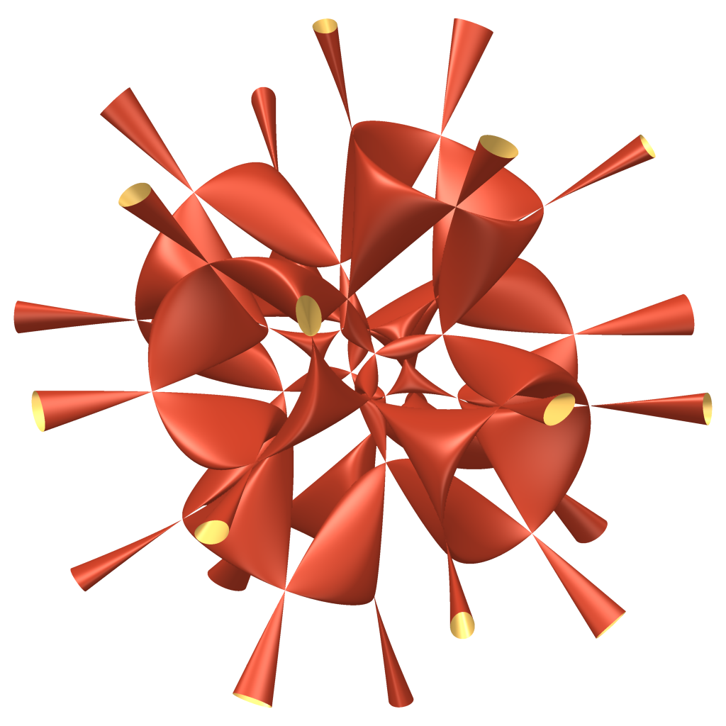
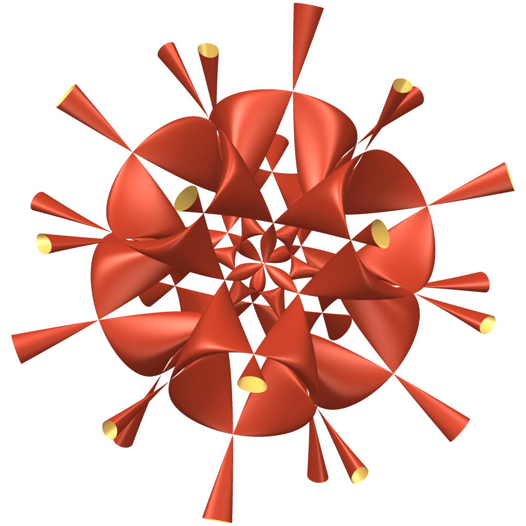
Figure I: Part of the real locus of ${\mathscr{Z}}(\varphi_{2})$ for $W=G_{28}={\mathrm{W}}(F_{4})$.

Examples 4.5 (The group ${\boldsymbol{G_{29}}}$).

Assume in this example, and only in this example, that $W=G_{29}$, in the version implemented by Jean Michel in the Chevie package of GAP3 [Mic]. Then it contains the symmetric group ${\mathfrak{S}}_{4}$ (viewed as the subgroup of ${\mathbf{G}}{\mathbf{L}}_{4}({\mathbb{C}})$ consisting of permutation matrices). We use the notation of Example 4.3 for elementary symmetric functions and evaluation at powers of the indeterminates.

(1) Recall that the Endraß octic [End] has degree $8$ and $168$ nodes and its automorphism group has order $16$. As shown in Table IV, ${\mathscr{Z}}(F_{u_{3}})$ is an irreducible surface in ${\mathbf{P}}^{3}({\mathbb{C}})$ with $160$ nodes and a group of automorphisms of order at least $1~{}\!920$, thus approaching Endraß’ record but with more symmetries. However, this surface has no real point. Up to a scalar, we have

$$F_{u_{3}}=\sigma_{1}[8]+3\sigma_{1}[2]^{2}\sigma_{2}[2]+2\sigma_{2}[4]-30\sigma_{1}[2]\sigma_{3}[2]+240\sigma_{4}[2].$$

It is still an open question to determine whether one can find a surface of degree $8$ in ${\mathbf{P}}^{3}({\mathbb{C}})$ with more than $168$ nodes (being aware that the maximal number of nodes cannot exceed $174$, see [Miy]).

(2) For the surface ${\mathscr{Z}}(F_{u_{2}})$, it can be shown with the software Singular that the singularities are all of type $T_{4,4,4}$ that is, are equivalent to the singularity $xyz+x^{4}+y^{4}+z^{4}$. Up to a scalar, we have

$$F_{u_{2}}=\sigma_{1}[2]^{4}-32\sigma_{1}[2]\sigma_{3}[2]+256\sigma_{4}[2].$$

Figure II shows part of the real locus of ${\mathscr{Z}}(F_{u_{2}})$.

(3) On the other hand, if we set

$$\varphi_{1}=\sigma_{1}[2]^{6}-\frac{3}{2}\sigma_{1}[2]^{4}\sigma_{2}[2]-78\sigma_{1}[2]^{2}\sigma_{2}[2]^{2}+\frac{585}{2}\sigma_{1}[2]^{3}\sigma_{3}[2]+208\sigma_{2}[2]^{3}$$

$$-990\sigma_{1}[2]\sigma_{2}[2]\sigma_{3}[2]+1710\sigma_{1}[2]^{2}\sigma_{4}+1350\sigma_{3}[2]^{2}-2880\sigma_{2}[2]\sigma_{4}[2],$$

we can check that $\varphi_{1}\in{\mathbb{C}}[V]^{W}$ and that:

• ${\mathscr{Z}}(\varphi_{1})$ has exactly $160$ singular points, which are all singularities of type $D_{4}$.

• ${\mathscr{Z}}_{\mathrm{sing}}(\varphi_{1})$ is a single $G_{29}$-orbit.

This shows that

$$\mu_{D_{4}}(12)\hskip 1.00006pt\mathop{\geqslant}\nolimits\hskip 1.00006pt160,$$ (4.6)

as announced in the introduction. This improves considerably known lower bounds (to the best of our knowledge, it was only known that $\mu_{D_{4}}(12)\hskip 1.00006pt\mathop{\geqslant}\nolimits\hskip 1.00006pt96$, see [Esc2]). Recall also that Miyaoka’s bound says that $\mu_{D_{4}}(12)\hskip 1.00006pt\mathop{\leqslant}\nolimits\hskip 1.00006pt198$. Figure III shows part of the real locus of ${\mathscr{Z}}(\varphi_{1})$.

(4) Let us keep going on with fundamental invariants of degree $12$. Let

$$\varphi_{2}=\sigma_{3}[2]\sigma_{1}[2]^{3}-4\sigma_{1}[2]\sigma_{2}[2]\sigma_{3}[2]+4\sigma_{1}[2]^{2}\sigma_{4}[2]+4\sigma_{3}[2]^{2}$$

(up to a scalar). Then $\varphi_{2}\in{\mathbb{C}}[V]^{W}$ is irreducible over ${\mathbb{C}}$ (this has been checked with Singular) and computations with Magma show that:

• ${\mathscr{Z}}_{\mathrm{sing}}(\varphi_{2})$ has pure dimension $1$ and is the union of $30$ lines.

• $G_{29}$ acts transitively on these $30$ lines.

• The set of points belonging to at least two of these $30$ lines has cardinality $60$, and splits into two $G_{29}$-orbits (one of cardinality $40$, the other of cardinality $20$).

Figure IV shows part of the real locus of ${\mathscr{Z}}(\varphi_{2})$. $\blacksquare$

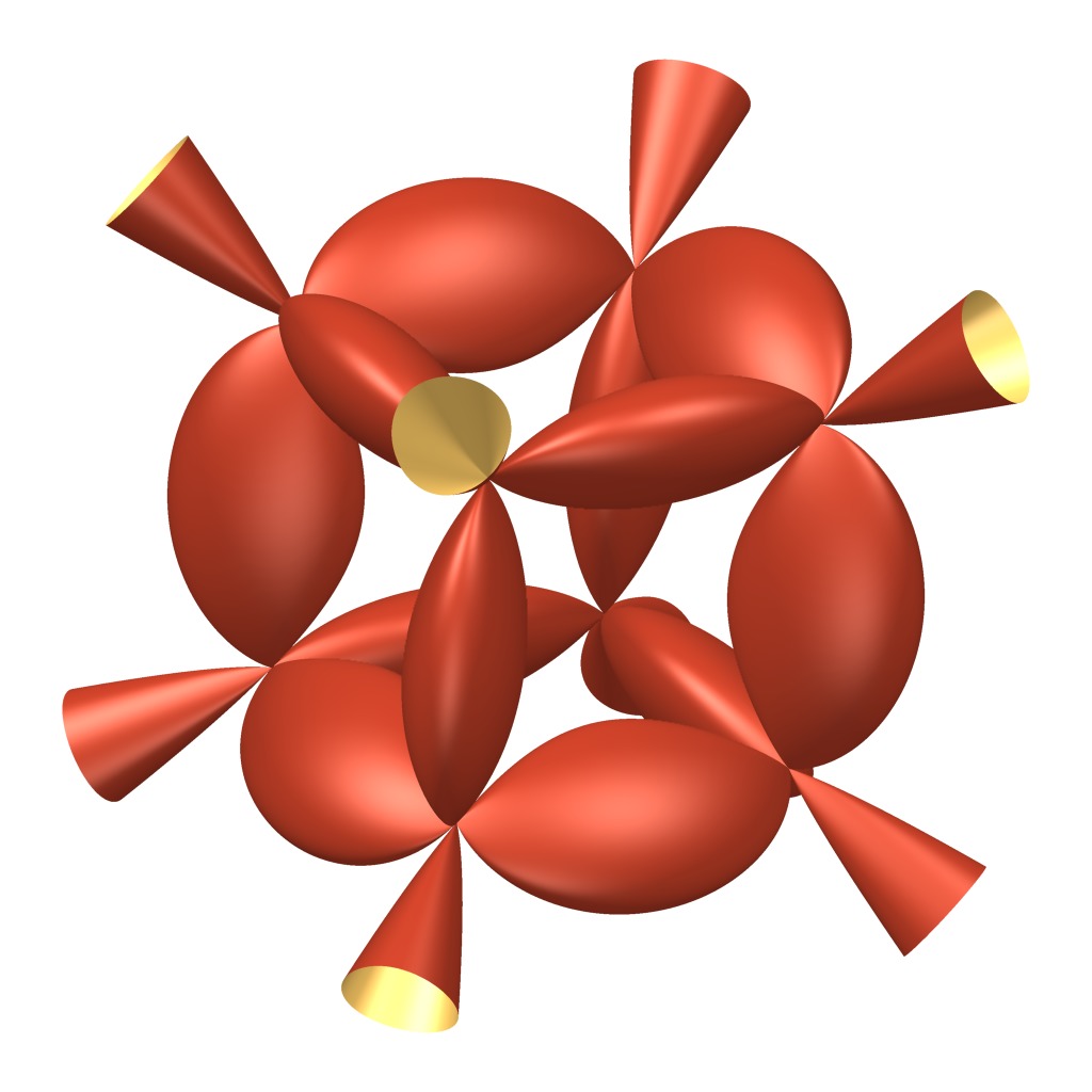
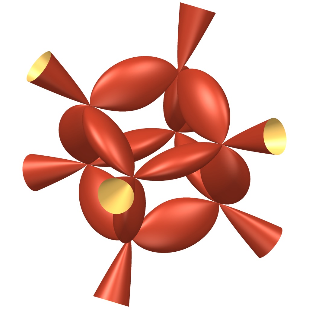
Figure II: Part of the real locus of ${\mathscr{Z}}(F_{u_{3}})$ for $W=G_{29}$.

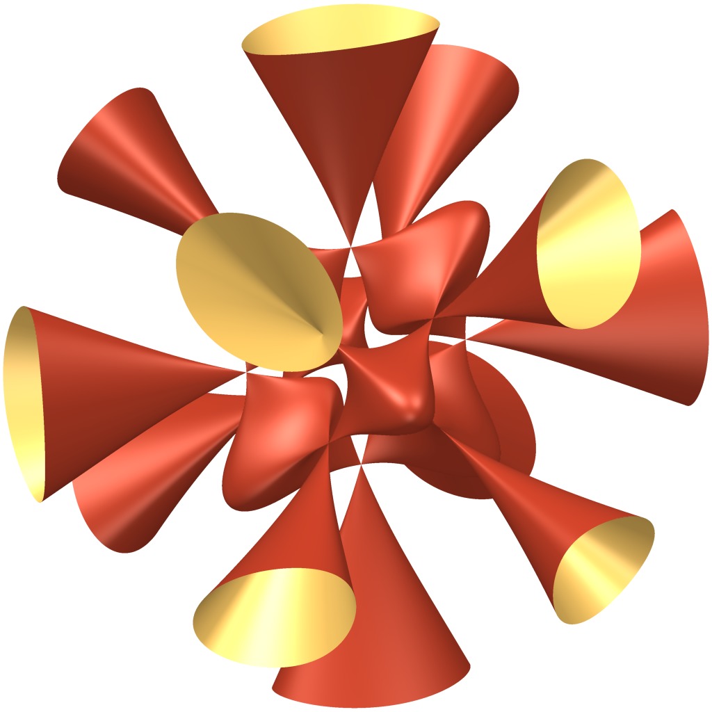
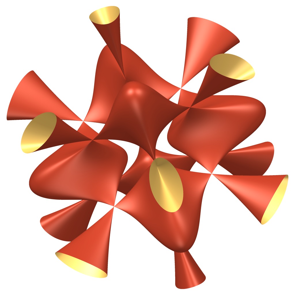
Figure III: Part of the real locus of ${\mathscr{Z}}(\varphi_{1})$ for $W=G_{29}$.

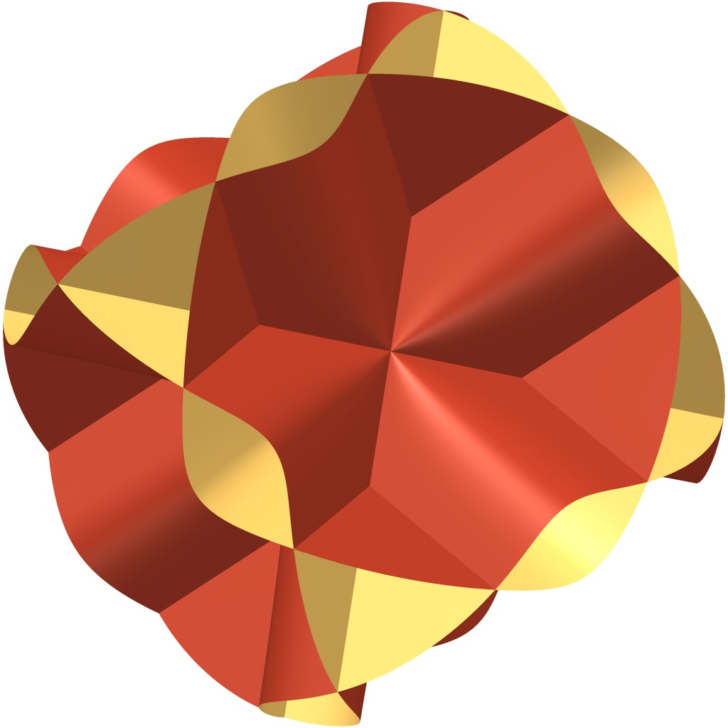
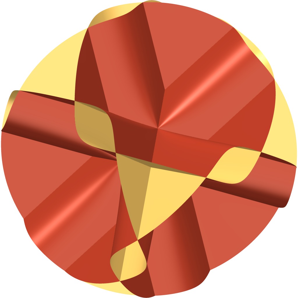
Figure IV: Part of the real locus of ${\mathscr{Z}}(\varphi_{2})$ for $W=G_{29}$.

Example 4.7 (The group ${\boldsymbol{G_{31}}}$).

Recall that the Chmutov surface [Chm] of degree $20$ has $2~{}\!926$ nodes and that an irreducible surface in ${\mathbf{P}}^{3}({\mathbb{C}})$ of degree $20$ cannot have more than $3~{}\!208$ nodes [Miy]. The third surface associated with $G_{31}$ in Table IV has “only” $1~{}\!920$ nodes and most of them are not real (contrary to the Chmutov surface). However, it has a big group of automorphisms (of order a least $11~{}\!520$). $\blacksquare$

5 Examples in higher dimension

Example 5.1 (The group ${\boldsymbol{G_{33}}}$).

Computations with Magma show that there are no fundamental invariant $f_{3}$ of degree $10$ of $G_{33}$ such that ${\mathscr{Z}}(f_{3})$ is singular [Bon2]. $\blacksquare$

Example 5.2 (Coxeter group of type ${\boldsymbol{E_{6}}}$).

Assume in this Example, and only in this Example, that $W=G_{35}$ is a Coxeter group of type $E_{6}$. Then $r=3$ and $(d_{1},d_{2},d_{3})=(2,5,6)$, so that any fundamental invariant of degree $6$ of $W$ is of the form $F_{u}=f_{3}+uf_{1}^{3}$ for some $u\in{\mathbb{C}}$. Computations with Magma show that [Bon2]:

• $U_{\mathrm{sing}}=U_{\mathrm{sing}}^{\mathrm{irr}}$ has cardinality $8$.

• For each $u\in U_{\mathrm{sing}}$, ${\mathscr{Z}}_{\mathrm{sing}}(F_{u})$ has dimension $0$, $W$ acts transitively on ${\mathscr{Z}}_{\mathrm{sing}}(F_{u})$, and all these singular points are nodes.

• The hypersurfaces ${\mathscr{Z}}(F_{u})$, $u\in U_{\mathrm{sing}}^{\mathrm{irr}}$, have respectively $27$, $36$, $135$, $216$, $360$, $432$, $1080$ and $1080$ singular points. $\blacksquare$

The other exceptional groups have been investigated but the computations are somewhat too long (note that $n\hskip 1.00006pt\mathop{\geqslant}\nolimits\hskip 1.00006pt5$).

6 The case of ${\boldsymbol{G_{32}}}$

   Hypothesis. We assume in this section, and only in this section, that $W$ is the primitive complex reflection group $G_{32}$.$A_{\displaystyle{A_{A}}}$

In Table IV, it is said that the surface ${\mathscr{Z}}(F_{u_{3}})$ attached to $G_{32}$ has $1~{}\!440$ singularities of type $D_{4}$. We give here a detailed account of this example, and show that it also produces surfaces of degree $8$ and $16$ with many singularities of type $D_{4}$. The Magma codes are contained in the arXiv version of this section [Bon1].

We need some more notation. If $f\in{\mathbb{C}}[x_{1},x_{2},x_{3},x_{4}]$ is homogeneous, we denote by $f[k]$ the homogeneous polynomial $f(x_{1}^{k},x_{2}^{k},x_{3}^{k},x_{4}^{k})$. Let $W_{1}$ be the subgroup of ${\mathbf{G}}{\mathbf{L}}_{4}({\mathbb{C}})$ generated by

$$s_{1}=\begin{pmatrix}0&1&0&0\\ 1&0&0&0\\ 0&0&1&0\\ 0&0&0&-1\\ \end{pmatrix},\quad s_{2}=\begin{pmatrix}1&0&0&0\\ 0&0&1&0\\ 0&1&0&0\\ 0&0&0&-1\\ \end{pmatrix}\quad\text{and}\quad s_{3}=\begin{pmatrix}-1&0&0&0\\ 0&1&0&0\\ 0&0&0&1\\ 0&0&1&0\\ \end{pmatrix}.$$

Let $\zeta_{3}$ (resp. $\zeta_{4}$) be a primitive third (resp. fourth) root of unity. Let $W_{2}$ be the subgroup of ${\mathbf{G}}{\mathbf{L}}_{4}({\mathbb{C}})$ generated by

$$s_{1}^{\prime}=\begin{pmatrix}0&1&0&0\\ 1&0&0&0\\ 0&0&1&0\\ 0&0&0&\zeta_{4}\\ \end{pmatrix},\quad s_{2}^{\prime}=\begin{pmatrix}1&0&0&0\\ 0&0&1&0\\ 0&1&0&0\\ 0&0&0&\zeta_{4}\\ \end{pmatrix}\quad\text{and}\quad s_{3}^{\prime}=\begin{pmatrix}-\zeta_{4}&0&0&0\\ 0&1&0&0\\ 0&0&0&1\\ 0&0&1&0\\ \end{pmatrix}.$$

Finally, let $W=W_{3}$ denote the subgroup of ${\mathbf{G}}{\mathbf{L}}_{4}({\mathbb{C}})$ generated by

$$s_{1}^{\prime\prime}=\begin{pmatrix}1&0&0&0\\ 0&1&0&0\\ 0&0&\zeta_{3}&0\\ 0&0&0&1\\ \end{pmatrix},\quad s_{2}^{\prime\prime}=\begin{pmatrix}\frac{\zeta_{3}+2}{3}&\frac{\zeta_{3}-1}{3}&\frac{\zeta_{3}-1}{3}&0\\ \frac{\zeta_{3}-1}{3}&\frac{\zeta_{3}+2}{3}&\frac{\zeta_{3}-1}{3}&0\\ \frac{\zeta_{3}-1}{3}&\frac{\zeta_{3}-1}{3}&\frac{\zeta_{3}+2}{3}&0\\ 0&0&0&1\\ \end{pmatrix},$$

$$s_{3}^{\prime\prime}=\begin{pmatrix}1&0&0&0\\ 0&\zeta_{3}&0&0\\ 0&0&1&0\\ 0&0&0&1\\ \end{pmatrix}\quad\text{and}\quad s_{4}^{\prime\prime}=\begin{pmatrix}\frac{\zeta_{3}+2}{3}&\frac{1-\zeta_{3}}{3}&0&\frac{1-\zeta_{3}}{3}\\ \frac{1-\zeta_{3}}{3}&\frac{\zeta_{3}+2}{3}&0&\frac{\zeta_{3}-1}{3}\\ 0&0&1&0\\ \frac{1-\zeta_{3}}{3}&\frac{\zeta_{3}-1}{3}&0&\frac{\zeta_{3}+2}{3}\\ \end{pmatrix}.$$

Commentaries. The following facts are checked using Magma, as explained in [Bon1]. Let ${\mathrm{Z}}(W_{i})$ denote the center of $W_{i}$. In all cases, it is isomorphic to a group of roots of unity acting by scalar multiplication. Then:

• The group $W_{1}$ has order $48$ and is isomorphic to the non-trivial double cover ${\mathbf{G}}{\mathbf{L}}_{2}({\mathbb{F}}_{\!3})$ of the symmetric group ${\mathfrak{S}}_{4}\simeq W_{1}/{\mathrm{Z}}(W_{1})$.

• The group $W_{2}$ has order $768$, contains a normal abelian subgroup $H$ of order $32$ and $W_{2}/H\simeq{\mathfrak{S}}_{4}$. The group $W_{2}/{\mathrm{Z}}(W_{2})$ has order $192$, but is not isomorphic to a Coxeter group of type $D_{4}$.

• The group $W_{3}$ is the complex reflection group denoted by $G_{32}$ in the Shephard–Todd classification [ShTo] (it has order $155~{}\!920$). Recall that the group $W_{3}/{\mathrm{Z}}(W_{3})$ is a simple group of order $25~{}\!920$ and is isomorphic to the derived subgroup of the Weyl group of type $E_{6}$ (i.e. to the derived subgroup of the special orthogonal group ${\mathbf{S}}{\mathbf{O}}_{5}({\mathbb{F}}_{\!3})$). It contains the group $W_{1}$ as a subgroup, as well as a subgroup of diagonal matrices isomorphic to $({\boldsymbol{\mu}}_{3})^{4}$, where ${\boldsymbol{\mu}}_{d}$ is the group of $d$-th roots of unity.

  Note that we have used the version of $G_{32}$ implemented by Michel in the Chevie package of GAP3 [Mic]. $\blacksquare$

If $\lambda=(\lambda_{1}\hskip 1.00006pt\mathop{\geqslant}\nolimits\hskip 1.00006pt\lambda_{2}\hskip 1.00006pt\mathop{\geqslant}\nolimits\hskip 1.00006pt\lambda_{3}\hskip 1.00006pt\mathop{\geqslant}\nolimits\hskip 1.00006pt\lambda_{4})$ is a partition of $8$ of length at most $4$, we denote by $\Omega_{\lambda}^{-}$ (resp. $\Omega_{\lambda}^{+}$) be the orbit of the monomial $x_{1}^{\lambda_{1}}x_{2}^{\lambda_{2}}x_{3}^{\lambda_{3}}x_{4}^{\lambda_{4}}$ under the action of $W_{1}$ (resp. the symmetric group ${\mathfrak{S}}_{4}$) and we set

$$m_{\lambda}^{\varepsilon}=\sum_{m\in\Omega_{\lambda}^{\varepsilon}}m$$

for $\varepsilon\in\{+,-\}$. Then $m_{\lambda}^{+}$ is the symmetric function traditionnally denoted by $m_{\lambda}$. If all the $\lambda_{i}$’s are even, then $m_{\lambda}^{-}=m_{\lambda}^{+}$ but note for instance that

$$m_{611}^{+}\neq m_{611}^{-} = x_{1}^{6}x_{2}x_{3}+x_{1}^{6}x_{2}x_{4}-x_{1}^{6}x_{3}x_{4}+x_{1}x_{2}^{6}x_{3}-x_{1}x_{2}^{6}x_{4}+x_{2}^{6}x_{3}x_{4}$$

$$+x_{1}x_{2}x_{3}^{6}+x_{1}x_{3}^{6}x_{4}-x_{2}x_{3}^{6}x_{4}-x_{1}x_{2}x_{4}^{6}-x_{1}x_{3}x_{4}^{6}-x_{2}x_{3}x_{4}^{6}.$$

Now, let

$$g\!\!\!\! = \!\!\!\!m_{8}^{-}-6m_{62}^{-}-60m_{611}^{-}+2~{}\!240m_{521}^{-}-14m_{44}^{-}+10~{}\!180m_{431}^{-}+40~{}\!412m_{422}^{-}$$

$$-23~{}\!440m_{4211}^{-}+111~{}\!980m_{332}^{-}+154~{}\!704m_{2222}^{-}.$$

By construction, $m_{\lambda}^{-}$ is invariant under the action of $W_{1}$ and so $g$ is invariant under the action of $W_{1}\simeq\tilde{{\mathfrak{S}}}_{4}$. One can check with Magma the following facts [Bon1, Proposition 1]:

Proposition 6.1.

If $1\hskip 1.00006pt\mathop{\leqslant}\nolimits\hskip 1.00006ptk\hskip 1.00006pt\mathop{\leqslant}\nolimits\hskip 1.00006pt3$, then the polynomial $g[k]$ is invariant under the action of $W_{k}$.

One can also check that $g[3]$ is the polynomial denoted by $F_{u_{3}}$ (suitably normalized) in Table IV (in the $G_{32}$ example).

Theorem 6.2.

The homogeneous polynomial $g$ satisfies the following statements:

• ${\mathscr{Z}}(g)$ is an irreducible surface of degree $8$ in ${\mathbf{P}}^{3}({\mathbb{C}})$ with exactly $44$ singular points which are all quotient singularities of type $D_{4}$.

• If $k\hskip 1.00006pt\mathop{\geqslant}\nolimits\hskip 1.00006pt1$, then ${\mathscr{Z}}(g[k])$ is an irreducible surface of degree $8k$, whose singular locus has dimension $0$ and contains at least $44k^{3}$ quotient singularities of type $D_{4}$.

• ${\mathscr{Z}}(g[2])$ is an irreducible surface of degree $16$ with exactly $472$ singular points: $24$ quotient singularities of type $A_{1}$, $96$ quotient singularities of type $A_{2}$ and $352$ quotient singularities of type $D_{4}$.

• ${\mathscr{Z}}(g[3])$ is an irreducible surface of degree $24$ in ${\mathbf{P}}^{3}({\mathbb{C}})$ with exactly $1~{}\!440$ singular points which are all quotient singularities of type $D_{4}$.

Remark 6.3.

Note that $g$ has coefficients in ${\mathbb{Q}}$ but the singular points of ${\mathscr{Z}}(g)$, ${\mathscr{Z}}(g[2])$ and ${\mathscr{Z}}(g[3])$ have coordinates in various field extensions of ${\mathbb{Q}}$, and most of the singular points are not real (at least in this model). $\blacksquare$

We now turn to the study of the singularities of the varieties ${\mathscr{Z}}(g[i])$ for $i\in\{1,2,3\}$. Note the following fact, checked using Magma [Bon1, Lemma 3], that will be used further:

Lemma 6.4.

If $1\hskip 1.00006pt\mathop{\leqslant}\nolimits\hskip 1.00006pti<j\hskip 1.00006pt\mathop{\leqslant}\nolimits\hskip 1.00006pt4$, then the closed subscheme of ${\mathbf{P}}^{3}({\mathbb{C}})$ defined by the homogeneous ideal $\langle g,\frac{\partial g}{\partial x_{i}},\frac{\partial g}{\partial x_{j}}\rangle$ has dimension $0$.

6.A Degree ${\boldsymbol{8}}$

The Magma computations leading to the proof of the statement (a) of Theorem 6.2 are detailed in [Bon1, §1]. Along these computations, the following facts are obtained (here, ${\mathscr{U}}$ denotes the open subset of ${\mathbf{P}}^{3}({\mathbb{C}})$ defined by $x_{1}x_{2}x_{3}x_{4}\neq 0$):

Proposition 6.5.

We have:

• $\dim{\mathscr{Z}}_{\mathrm{sing}}(g)=0$, so ${\mathscr{Z}}(g)$ is irreducible.

• ${\mathscr{Z}}_{\mathrm{sing}}(g)$ is contained in ${\mathscr{U}}$.

• The group $W_{1}$ has $3$ orbits in ${\mathscr{Z}}_{\mathrm{sing}}(g)$, of respective length $8$, $12$ and $24$.

Note that the points in the $W_{1}$-orbit of cardinality $8$ are the only real singular points of ${\mathscr{Z}}(g)$. Figure V shows part of the real locus of ${\mathscr{Z}}(g)$.

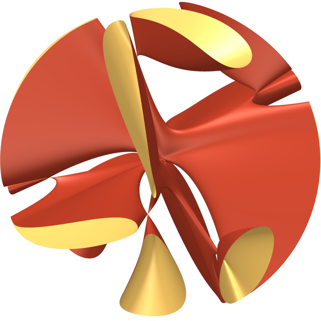
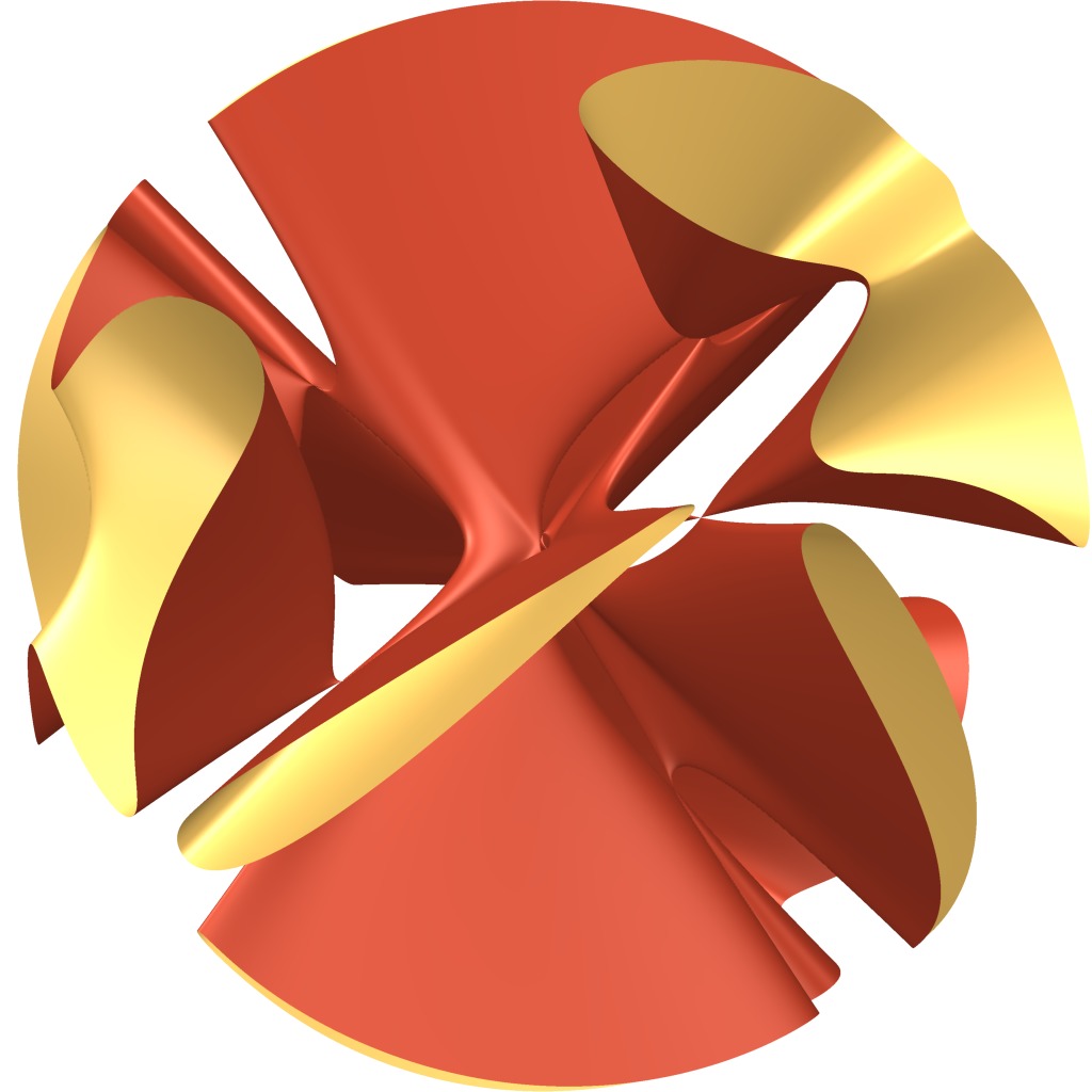
Figure V: Part of the real locus of ${\mathscr{Z}}(g)$

6.B Degree ${\boldsymbol{8k}}$

Let ${\mathscr{U}}$ denote the open subset of ${\mathbf{P}}^{3}({\mathbb{C}})$ defined by $x_{1}x_{2}x_{3}x_{4}\neq 0$ and let $\sigma_{\!k}:{\mathbf{P}}^{3}({\mathbb{C}})\rightarrow{\mathbf{P}}^{3}({\mathbb{C}})$, $[x_{1};x_{2};x_{3};x_{4}]\mapsto[x_{1}^{k};x_{2}^{k};x_{3}^{k};x_{4}^{k}]$. The restriction of $\sigma_{\!k}$ to a morphism ${\mathscr{U}}\rightarrow{\mathscr{U}}$ is an étale Galois covering, with group $({\boldsymbol{\mu}}_{k})^{4}/\Delta{\boldsymbol{\mu}}_{k}$ (here, $\Delta:{\boldsymbol{\mu}}_{k}\hookrightarrow({\boldsymbol{\mu}}_{k})^{4}$ is the diagonal embedding). We have ${\mathscr{Z}}(g[k])=\sigma_{\!k}^{-1}({\mathscr{Z}}(g))$.

Let us first prove that ${\mathscr{Z}}(g[k])$ is irreducible. We may assume that $k\hskip 1.00006pt\mathop{\geqslant}\nolimits\hskip 1.00006pt2$, as the result has been proved for $k=1$ in the previous section. Recall that

$$\frac{\partial g[k]}{\partial x_{i}}=kx_{i}^{k-1}(\frac{\partial g}{\partial x_{i}}\circ\sigma_{\!k}),$$

so the singular locus of ${\mathscr{Z}}(g[k])$ is contained in

$$\{p_{1},p_{2},p_{3},p_{4}\}\cup\Bigl{(}\bigcup_{i\neq j}\sigma_{\!k}^{-1}({\mathscr{Z}}_{i,j})\Bigr{)},$$

where $p_{i}=[\delta_{i1};\delta_{i2};\delta_{i3};\delta_{i4}]$ (and $\delta_{ij}$ is the Kronecker symbol) and ${\mathscr{Z}}_{i,j}$ is the subscheme of ${\mathbf{P}}^{3}({\mathbb{C}})$ defined by the ideal $\langle g,\frac{\partial g}{\partial x_{i}},\frac{\partial g}{\partial x_{j}}\rangle$ (and which has dimension $0$ by Lemma 6.4). Since $\sigma_{\!k}$ is finite, this implies that ${\mathscr{Z}}_{\mathrm{sing}}(g[k])$ has dimension $0$, so ${\mathscr{Z}}(g[k])$ is irreducible.

Now, $\sigma_{\!k}:{\mathscr{U}}\rightarrow{\mathscr{U}}$ is étale and the singular locus of ${\mathscr{Z}}(g)$ is contained in ${\mathscr{U}}$ (see Proposition 4(b)). Therefore, the $44$ singularities of ${\mathscr{Z}}(g)$ lift to $44k^{3}$ singularities in ${\mathscr{Z}}(g[k])\cap{\mathscr{U}}$ of the same type, i.e. quotient singularities of type $D_{4}$. This proves the statement (b) of Theorem 6.2.

Note that, for $k=2$, $3$ and $4$ (and maybe for bigger $k$) we will prove in the next sections that ${\mathscr{Z}}(g[k])$ contains singular points outside of ${\mathscr{U}}$.

6.C Degree ${\boldsymbol{16}}$

Using the morphism $\sigma_{\!2}$ defined in the previous section, we get that ${\mathscr{Z}}(g[2])\cap{\mathscr{U}}$ has exactly $352$ singular points, which are all quotient singularities of type $D_{4}$. The other singularities are determined thanks to Magma computations that are detailed in [Bon1, §3], and which confirm the statement (c) of Theorem 6.2. Note that we also need the software Singular [DGPS] for computing some Milnor numbers and identifying the singularity $A_{2}$. Note also that $W_{2}$ acts transitively on the $24$ quotient singularities of type $A_{1}$ and also acts transitively on the $96$ quotient singularities of type $A_{2}$. Figure VI shows part of the real locus of ${\mathscr{Z}}(g)$.

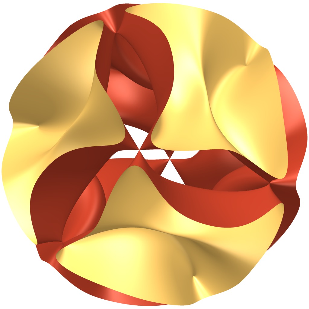
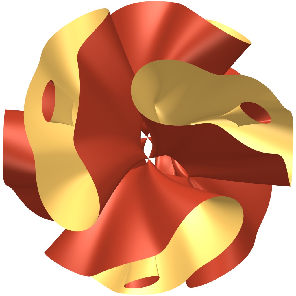
Figure VI: Part of the real locus of ${\mathscr{Z}}(g[2])$

6.D Degree ${\boldsymbol{24}}$

Using the morphism $\sigma_{\!3}$ defined in Section 6.B, we get that ${\mathscr{Z}}(g[3])\cap{\mathscr{U}}$ has exactly $44\times 3^{3}=1~{}\!188$ singular points, which are all quotient singularities of type $D_{4}$. The other singularities are determined thanks to Magma computations that are detailed in [Bon2] or [Bon1, §4], and which confirm the statement (d) of Theorem 6.2. Note also that, in the given model, the surface ${\mathscr{Z}}(g[3])$ has only $32$ real singular points: Figure VII gives partial views of its real locus.

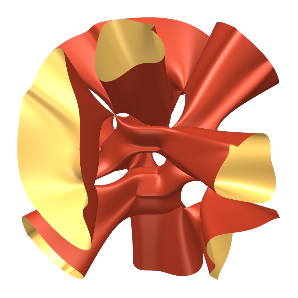
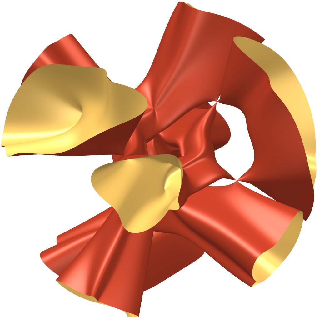
Figure VII: Part of the real locus of ${\mathscr{Z}}(g[3])$

6.E Complements

From Section 6.B, we deduce that ${\mathscr{Z}}_{\mathrm{sing}}(g[4])$ has $2~{}\!816$ quotient singularities of type $D_{4}$ lying in the open subset ${\mathscr{U}}$ and it can be checked that it has $432$ other singular points not lying in ${\mathscr{U}}$, for which we did not determine the type.

Acknowledgements. This paper is based upon work supported by the National Science Foundation under Grant No. DMS-1440140 while the author was in residence at the Mathematical Sciences Research Institute in Berkeley, California, during the Spring 2018 semester. The hidden computations which led to the discovery of the polynomial $g$ were done using the High Performance Computing facilities of the MSRI.

I wish to thank warmly Alessandra Sarti, Oliver Labs and Duco van Straten for useful comments and references and Gunter Malle for a careful reading of a first version of this paper. Figures were realized using the software SURFER [Sur].