Radio observations of planetary nebulae: no evidence for strong radial density gradients

Abstract

Radio continuum observations trace thermal emission of ionized plasma in planetary nebulae and bring useful information on nebular geometries. A model of homogeneous sphere or shell cannot fit the nebular spectra and brightness temperatures. Two alternative models have been proposed in the literature: the first one consists of two homogeneous components, while the other one is a model of a shell with a significant radial density gradient. On the other side, prolate ellipsoidal shell model can successfully fit the surface brightness distribution of selected objects. We verify the existing models using data collected in radio surveys covering wide range of frequencies. In about 50% cases, density gradient can be excluded, and none of the remaining objects could be confirmed. None of the observed planetary nebulae show the spectral index of 0.6 in the optically thick part of the spectrum, which is a value predicted for a shell containing strong radial density gradient. Radio spectra can be fitted with a model of prolate ellipsoidal shell, but also by a shell containing temperature variations in planetary nebulae. At least eight planetary nebulae show two component spectra, with one compact component showing much higher optical thickness than the other one. Unexpectedly, a group of planetary nebulae with lowest surface brightness show non-negligible optical thickness. Their emission comes from compact and dense structures, comprising only small part of total nebular mass.

1 Introduction

Low and intermediate mass stars ($1-8\,\textrm{M}_{\odot}$) play a vital role in the chemical evolution of the Galaxy (Marigo, 2001). Up to 90% of their initial mass returns to the interstellar medium, most of it during the asymptotic giant branch (AGB) phase of their evolution.

After a long phase of steady hydrogen burning on the main sequence, hydrogen is exhausted in the center of the star and nuclear burning proceeds in a shell around a helium core. The star ascends the red giant branch in the Hertzsprung-Russell diagram. Subsequently, helium ignites in the core. After helium is exhausted in the core, helium burning proceeds in a shell on the top of carbon-oxygen core. The star ascends the asymptotic giant branch.

The main site of nucleosynthesis at the end of the AGB phase is the helium burning shell, separated from the hydrogen burning shell by the intershell region. Helium burning activates during the thermal pulse (helium flash), when enough helium is accumulated in quiescent hydrogen burning. The material synthesized during a thermal pulse is subsequently dredged up to the surface by the convective envelope.

Thermal pulses trigger heavy mass loss. When the envelope mass is reduced to ${\sim}10^{-3}\,M_{\odot}$, the star begins to evolve very quickly to higher effective temperatures. Heavy mass loss terminates, and the slow and dense AGB wind is being compressed by a fast wind from the central star, which creates a central cavity. The density profile of the shell is further modified by the passage of the ionization front. A planetary nebula (PN, plural PNe) becomes visible as a result of ionization and wind interaction.

2 Radio emission of planetary nebulae

Planetary nebulae are detectable in a broad range of the electromagnetic spectrum, from UV or even X rays to radio frequencies. Continuum radio emission originates from thermal free-free emission of electrons (Pazderska et al., 2009; Chhetri et al., 2015). Radio observations trace all the ionized ejecta in the PN and give information on the nebular structure and physical parameters unaffected by extinction. This in turn can help to reveal the mass loss history of the star.

Spherically symmetric models cannot fit the observations. PNe show an excess of the 5 GHz/1.4 GHz flux ratio with respect to a model of a homogeneous spherical shell. Siódmiak & Tylenda (2001) introduced a model consisting of two components to fit the observations.

On the other hand, Phillips (2007) claimed that at least $10-20\%$ of PNe are associated with strong density gradients, which can explain the observed 5 GHz/1.4 GHz flux indices. For a shell with the density varying with radius $n_{e}(r)\propto r^{-2}$ the spectrum has a slope of ${\sim}0.6$ in the range of frequencies.

Gruenwald & Aleman (2007) were able to reproduce a range of spectral indices without introducing the initial density gradient, however, they analyzed the spectral indices limited to the frequency interval of 0.6 to 0.4 GHz.

The analysis using 5 GHz/1.4 GHz flux ratio by Siódmiak & Tylenda (2001) and Phillips (2007) did not lead to conclusive results. A prolate ellipsoidal shell was used by Masson (1990) and Aaquist & Kwok (1996) to fit radio images of PNe. The prolate ellipsoidal shell, viewed at different angles, can reproduce variety of observed nebular morphologies.

With the advent of many radio surveys, more data is available for different frequencies in addition to 5 GHz and 1.4 GHz fluxes, widely used in previous studies. We take advantage of recently published catalogs of radio fluxes covering low and high frequency region to further constrain the proposed models. New data helped us to constrain the slope of radio spectra at optically thick part, which can verify the existence of strong density gradients. We also attempted to fit prolate ellipsoidal shell model and models with electron temperature varying across the nebula to the observed spectral indices.

3 Data

Table 1: Radio continuum observations used for modeling of nebular spectra.

frequency [GHz]	sky coverage	sensitivity [mJy/beam]	beam size	reference
0.15	$\delta>-56^{\circ}$	25	$20^{\prime\prime}\textrm{or}\,25^{\prime\prime}\times 25^{\prime\prime}$	Intema et al. (2017)
0.2	$\delta<+30^{\circ}$ & $|b|>10^{\circ}$	6.7	see reference	Hurley-Walker et al. (2017)
0.325	$\delta>+28^{\circ}$	30	$54^{\prime\prime}\times 54^{\prime\prime}\mathrm{cosec}\,\delta$	Rengelink et al. (1997)
0.330	$+42<l<+92$, $|b|<1.6^{\circ}$	10	$1^{\prime}\times 1^{\prime}\mathrm{cosec}\,\delta$	Taylor et al. (1996)
0.352	$-26^{\circ}<\delta<-9^{\circ}$	18	$54^{\prime\prime}\times 54^{\prime\prime}\mathrm{cosec}\,\delta$	De Breuck et al. (2002)
0.365	$71.5^{\circ}>\delta>-35^{\circ}$	400	see reference	Douglas et al. (1996)
0.843	$\delta<-30^{\circ},|b|>10^{\circ}$	18 (8 for $\delta<-50$)	$45^{\prime\prime}\times 45^{\prime\prime}\mathrm{cosec}\,\delta$	Mauch et al. (2003)
0.843	$|b|<-10^{\circ},245^{\circ}<l<365^{\circ}$	10 (6 for $\delta<-50$)	$45^{\prime\prime}\times 45^{\prime\prime}\mathrm{cosec}\,\delta$	Murphy et al. (2007)
1.4	$\delta>-40^{\circ}$	2.5	$45^{\prime\prime}$	Condon et al. (1998)
1.4	dedicated survey	see reference	$3.8^{\prime\prime}\times 5.5^{\prime\prime}$	Isaacman (1984)
1.5	dedicated survey	see reference	see reference	Zijlstra et al. (1989)
4.85	$0^{\circ}<\delta<75^{\circ}$	25	$3.6^{\prime}\times 3.4^{\prime}$	Gregory et al. (1996)
4.85	$-87.5^{\circ}<\delta<10^{\circ}$	35	$4.2^{\prime}$	Griffith & Wright (1993)
4.85	dedicated survey	see reference	$2.8^{\prime\prime}\times 1.5^{\prime\prime}$	McConnell (2012)
5	dedicated survey	see reference	$4.9^{\prime\prime}\times 6.5^{\prime\prime}$	Isaacman (1984)
5	dedicated survey	see reference	see reference	Zijlstra et al. (1989)
5	dedicated survey	see reference	$0.5^{\prime\prime}$	Aaquist & Kwok (1990)
5	$\delta<27^{\circ}$	see reference	$4.5^{\prime\prime}$	Milne & Aller (1975)
5	$\delta<0^{\circ}$	40	see reference	Murphy et al. (2010)
8	$\delta<0^{\circ}$	40	see reference	Murphy et al. (2010)
8.6	dedicated survey	see reference	$1.3^{\prime\prime}\times 0.9^{\prime\prime}$	McConnell (2012)
14.7	$\delta<27^{\circ}$	see reference	$2.1^{\prime\prime}$	Milne & Aller (1982)
15	dedicated survey	see reference	see reference	Zijlstra et al. (1989)
15	dedicated survey	see reference	$0.1^{\prime\prime}$	Aaquist & Kwok (1996)
16	$|b|\leq 5,170^{\circ}>l>76^{\circ}$	16	$3^{\prime}$	Perrott et al. (2015)
20	$\delta<0^{\circ}$	40	see reference	Murphy et al. (2010)
30	$\delta>-15^{\circ}$	20	$1.2^{\prime}$	Pazderska et al. (2009)
30	all sky	427	$32^{\prime}$	Planck Collaboration (2016)
31	dedicated survey	20	$45.2^{\prime\prime}$	Casassus et al. (2007)
43	dedicated survey	50	$54^{\prime\prime}$	Umana et al. (2008)
44	all sky	692	$27^{\prime}$	Planck Collaboration (2016)
70	all sky	501	$13.2^{\prime}$	Planck Collaboration (2016)
100	all sky	269	$9.7^{\prime}$	Planck Collaboration (2016)
143	all sky	177	$7.2^{\prime}$	Planck Collaboration (2016)
217	all sky	152	$4.9^{\prime}$	Planck Collaboration (2016)
353	all sky	304	$4.9^{\prime}$	Planck Collaboration (2016)
353	dedicated survey	71	$14^{\prime\prime}$	Di Francesco et al. (2008)

We searched for archival radio observations of PNe having at least three observations at different frequencies in total, including at least one observation in low or high frequency surveys to ensure wide coverage in frequencies.

Low frequency surveys between 150 and 352 MHz were carried on the Westerbork Synthesis Radio Telescope (Rengelink et al., 1997; Taylor et al., 1996; De Breuck et al., 2002), Giant Metrewave Radio Telescope (TGSS survey, Intema et al., 2017), Murchison Widefield Array (GLEAM survey, Hurley-Walker et al., 2017), and the Texas interferometer (Douglas et al., 1996). High frequency surveys were carried by Pazderska et al. (2009), Casassus et al. (2007), Umana et al. (2008), and the Planck Collaboration (2016). For intermediate frequencies we used data from surveys which derived fluxes with accuracy ${\leq}10\%$. The data are summarized in Table 1. We used SIMBAD database (Wenger et al., 2000) to identify spurious background sources.

We used nebular diameters from Frew et al. (2016). Radio diameters available in the literature become unreliable for small nebulae are less certain than optical diameters (Siódmiak & Tylenda, 2001). Frew et al. (2016) measured diameters for the emission region at the 10% level of the surface brightness, which should represent the shell contributing most of the flux in radio. In the case of non-spherical PNe, we adopted the geometric mean of the two axes.

4 Modeling of radio spectra

For an isothermal nebula the radio flux $S_{\nu}$ is given by

$$S_{\nu}=\frac{2\nu{{}^{2}}kT_{e}}{c^{2}}(1-e^{-\tau_{\nu}})\Omega$$ (1)

and optical thickness of the nebula $\tau_{\nu}$

$$\tau_{\nu}=5.44\times 10^{-2}T_{e}^{-1.5}\nu^{-2}g_{ff}(\nu,T_{e})\int n(H^{+})n_{e}dS$$ (2)

where $T_{e}$ is electron temperature, $\Omega$ is the solid angle, $n(H^{+})$ and $n_{e}$ are proton and electron density, respectively. The Gaunt factor is given by $g_{ff}$. Emission measure $EM=\int n_{e}\,n(H^{+})\,dS$ is integrated along the line of sight. van Hoof et al. (2014) provided accurate values of the Gaunt factor $g_{ff}$.

We used five different models to fit observations: a homogeneous sphere, a cylindrical shell seen along its axis, a spherical shell with uniform density distribution, a spherical shell containing radial density gradient, and a prolate ellipsoidal shell. We also checked if $T_{e}$ variations in a PN could fit the observations.

4.1 Model A: homogeneous sphere

As a first approximation, we fitted a model of a homogeneous sphere. There are three free parameters in equations 1 and 2: $\Omega$, $T_{e}$, and $EM$. $EM$ primarily determines the turnover frequency $\nu$ of the PN spectrum for which $\tau_{\nu}{\sim}1$. The optically thin part of the spectrum has a spectral index of about $-0.1$. The absolute flux is proportional to $EM$. The optically thick part of the spectrum has a spectral index of 2. The absolute flux is proportional to $T_{e}$. Additionally, $\Omega$ scales the absolute flux in the whole range of the spectrum. $EM$ and $T_{e}$, can be measured unambiguously when the radio spectrum covers both optically thick and thin emission. This is the case for most of PNe studied by us, which show decline of the flux due to increasing optical thickness at lowest frequencies.

Model A in most cases gave electron temperatures significantly lower than ${\sim}10^{4}\,K$, expected for photo ionized nebula in equilibrium (Fig. 1). Such low temperatures contradict optical observations and physics of PNe. Higher $T_{e}$, however, would overestimate the flux in optically thick region in model A. Thus, model A is not relevant for most of PNe.

4.2 Model B: homogeneous shell

In order to derive more physically plausible models, we fixed $T_{e}$ to the value derived from optical spectra $T_{opt}$ (Cahn et al., 1992). We used a model of uniform sphere, but with a central cavity defined by the ratio of the inner to outer radius $\eta_{B}=R_{in}/R$. The fitted parameters in model B were $\eta_{B}$ and $EM$.

The shell model with ${\eta}_{B}{\approx}1$ shows strong limb brightening. The $EM$ reaches the highest value at the projected distance of $R_{in}$ from the center of the PN and is low elsewhere, which may reproduce the observations. Model B with ${\eta}_{B}{\approx}1$ would require a very high density and would produce ring shaped PNe. On the other side, model B with ${\eta}_{B}{\approx}0$ is similar to model A.

The fitted $EM$ reproduced well the flux density but was too low to reproduce the turnover frequency in many cases (Fig. 1). Higher $EM$ would fit the turnover frequency better, but also would overestimate the absolute flux in optically thin part of the spectrum. Thus, model B is not relevant for most of PNe.

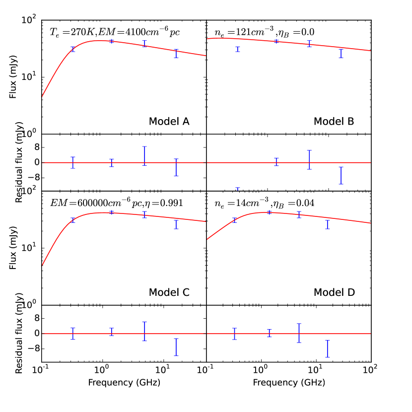
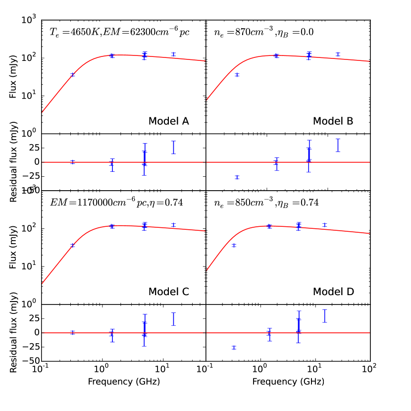
Figure 1: Four fits to the radio spectra of PN NGC 6842 (top) and IC 4634 (bottom) using models A, B, C, and D. The derived parameters for each model are shown. Lower panels show the residuals of the fits.

4.3 Model C: homogeneous cylindrical shell

We introduced the $(1-\eta^{2})$ factor in equation 1 so that we could increase $EM$ to achieve a good fit of the turnover region and simultaneously scale down the absolute flux:

$$S_{\nu}=\frac{2\nu{{}^{2}}kT_{e}}{c^{2}}(1-e^{-\tau_{\nu}})\Omega(1-\eta^{2})$$ (3)

where fitted parameters are $\eta$ and $EM$. The $\eta$ parameter is defined as the ratio of the projected inner to outer radius $R_{in}/R$.

Model C reproduced most of the spectra very well. It can be interpreted as a cylindrical shell seen along its axis, with the ratio of the internal to external radii defined by $\eta$. Model C can be relevant as a first approximation for some PNe, including the well known NGC 6720, which shows a disk seen pole on (O’Dell et al., 2013). Assuming random orientation of PNe in space, this model cannot account for most of PNe.

However, we find this model useful, as it is sensitive to the most optically thick part of the PN. The $\eta$ parameter gives information on surface brightness distribution of a PN. PNe with $\eta{\approx}0$ can be fit equally well using model A. Almost all PNe require $\eta>0$ (Fig. 6). Low surface brightness PNe need $\eta$ very close to 1. High value of $\eta$ indicates, that a small region with high $EM$ dominates in radio.

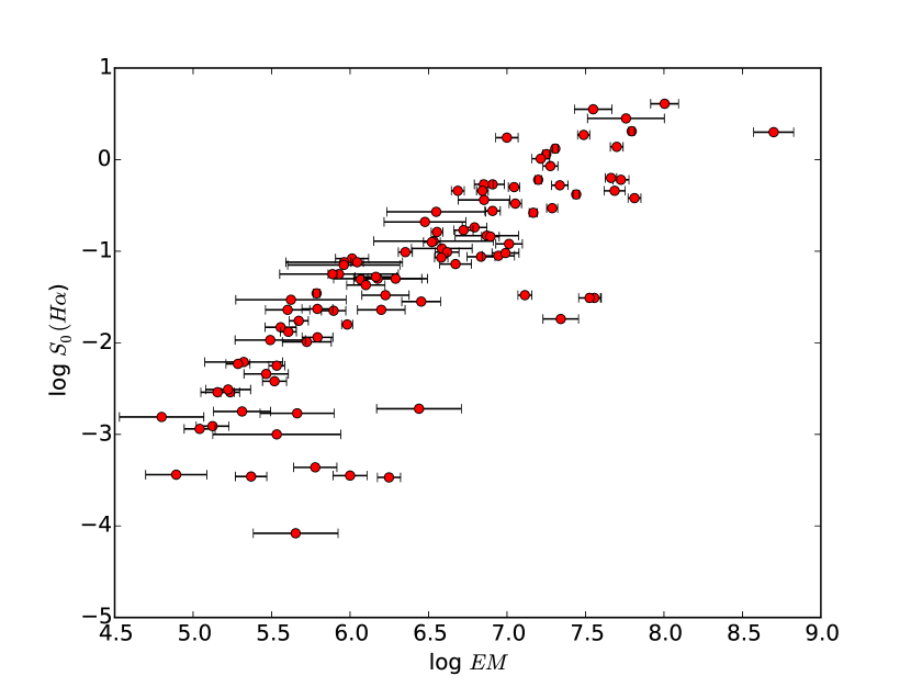
Figure 2: Emission measure vs $\textrm{H}{\alpha}$ surface brightness in observed PNe.

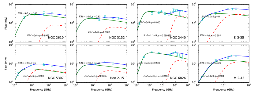
Figure 3: PNe showing two components in their spectra. Dashed red and green lines show separate components, blue line shows the sum of both components.

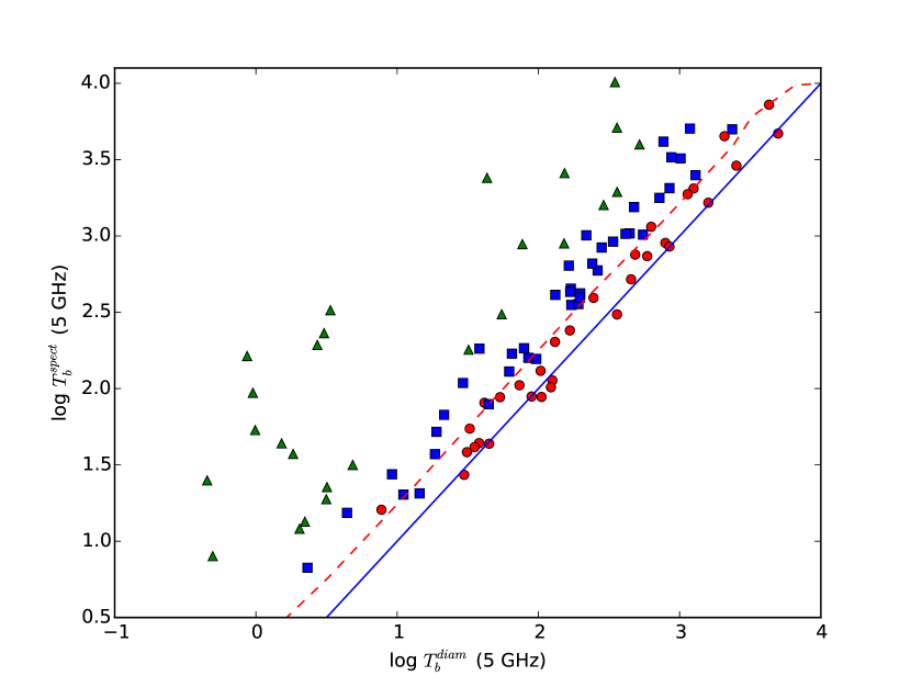
Figure 4: Brightness temperatures determined from measured diameter and flux and from radio spectra. PNe are split into three groups: $\eta<0.5$ (red circles), $0.5<\eta<0.9$ (blue squares), and $\eta>0.9$ (green triangles). Dashed red curve shows Model E for $a/b=3$, $t/b=0.1$, and $i=0^{\circ}$, and blue solid curve shows $T_{b}^{diam}=T_{b}^{spec}$ relation.

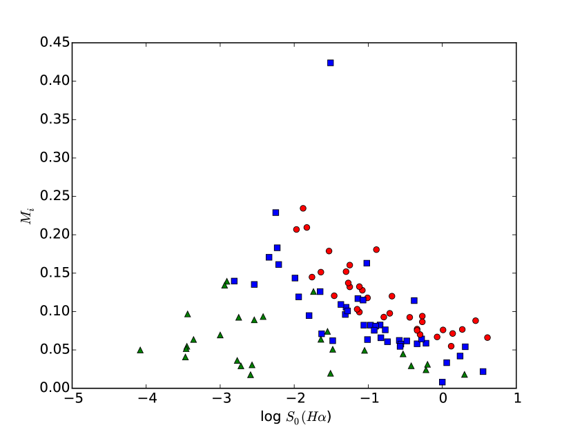
Figure 5: Ionized mass vs dereddened $H\alpha$ surface brightness.

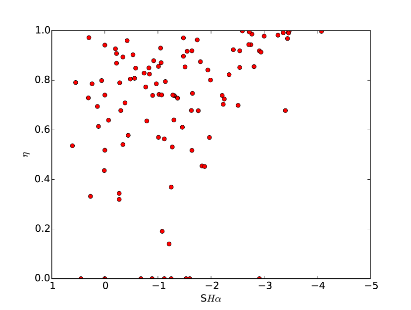
Figure 6: Diagram showing $\eta$ vs $\textrm{H}\alpha$ surface brightness.

Fig. 2 presents the relation between emission measure derived in model C and dereddened $\mathrm{H}{\alpha}$ surface brightness (Frew et al., 2016). As expected, $EM$ decreases with $S_{0}(\mathrm{H}\alpha)$, but unexpectedly this tendency is not held for PNe with the lowest surface brightnesses.

We also used a model consisting of two components, fitting two different values of $EM$ and $\eta$. In eight cases two components improves the fit significantly (Fig. 3). One of the components has much higher turnover frequency and a flux comparable to the second component. This indicates much higher $EM$ of the order of $10^{8}\,\mathrm{c}m^{-6}\,pc$, which could indicate a compact and dense (possibly cool) component in a PN.

In the appendix we list $EM$ and $\eta$ fitted to equation 3. In addition, we present optical depth at 5 GHz, brightness temperature at 5 GHz derived from fitting the spectrum $T_{b}^{spect}=T_{e}\times(1-e^{-{\tau}_{5GHz}})$, and from $T_{b}^{diam}=73.87\,F_{5GHz}/{\Theta}^{2}$, where $\Theta$ is the diameter of the PN measured in arcsec, and $F_{5GHz}$ is flux at 5 GHz measured in mJy.

$T_{b}^{spect}$ is systemically higher than $T_{b}^{diam}$ (Fig. 4). For uniform brightness distribution, corresponding to $\eta=0$, $T_{b}^{spect}=T_{B}^{diam}$. For non uniform brightness distribution, $T_{b}^{spect}>T_{B}^{diam}$. The ratio of $T_{b}^{spect}/T_{B}^{diam}$ in Model C simply depends on $\eta$: $T_{b}^{spect}/T_{B}^{diam}=1-\eta^{2}$.

We derived ionized masses using distances derived by Frew et al. (2016) and emission measures from radio spectra using model C. Ionized masses increase with decreasing surface brightness down to $\log(S_{o}(\mathrm{H}{\alpha}))=-2$ (Fig. 5) which reflects the progressing ionization in the nebulae (Frew et al., 2016). For lower surface brightness most of the observed PNe have $\eta>0.9$. Fig. 5 includes only PNe with reliable determination of $EM$, so low surface brightness PNe which are optically thin in radio are not included.

4.4 Model D: a shell with a density gradient $\beta=2$

We also used the modified model of power-law distribution by Olnon (1975) for $n_{e}=n_{o}(r/(\eta_{B}\times R))^{-\beta}$ for $\eta_{B}\times R>r>R$, $n=0$ for $r\leq\eta_{B}\times R$, and $\beta=2$. This density distribution can result from a steady-state wind lasting for a finite time interval. In this model we fitted $\eta$ and $n_{o}$.

Model D results in the flat spectrum in an optically thin part and in a spectral index of 0.6 in partially optically thick part, and an index of 2 in the optically thick part. The range of spectrum where spectral index is 0.6 depends on the value of $\eta_{B}$: the lower $\eta_{B}$, the larger range of frequencies where the spectral index of 0.6 is observed.

4.5 Model E: prolate ellipsoidal shell

Surface radio brightness distribution suggests that a model of a prolate ellipsoidal shell can be representative for most of PNe (Masson, 1990; Aaquist & Kwok, 1996). The inner and outer shell are defined as ellipsoids with minor and major axes of $(a,b)$ and $(a+t,b+t)$. Electron density depends on the incident flux, so that $n_{e}^{2}\times t$ is inversely proportional to the inner radius.

Due to large parameter space (inclinaton angle $i$, $a/b$ ratio, $t$, $n_{e}$), we did not use Model E to fit individual PNe, but to fit spectral indices and brightness temperatures.

4.6 Model F: temperature stratification

We also explored the influence of temperature stratification on the radio spectra of PNe. We assumed a spherical model with $T_{e}$ of 2500 K in the central region and 10000 K elsewhere, and a model with $T_{e}$ of 1000 K in the outer 20% radius and 10000 K inside. The temperature stratification is set arbitrarily. Again, we did not use this model for individual PNe, but rather to fit all PNe in the brightness temperature – spectral index diagrams.

5 Discussion

5.1 Spectral indices

A diagram of spectral indices vs $T_{b}$ reveal an excess of the observed flux ratios with respect to model A and B (Fig. 7, 8). The excess does not depend on the nebular diameter nor on the instrument used (Fig. 9), except for Milne & Aller (1975), where the fluxes appear to be correlated with nebular size. Data by Milne & Aller (1982) at higher frequencies show a similar problem. The data published by Perrott et al. (2015) appear to be underestimated. Apart from that the different instruments used does not seem to affect the observed indices.

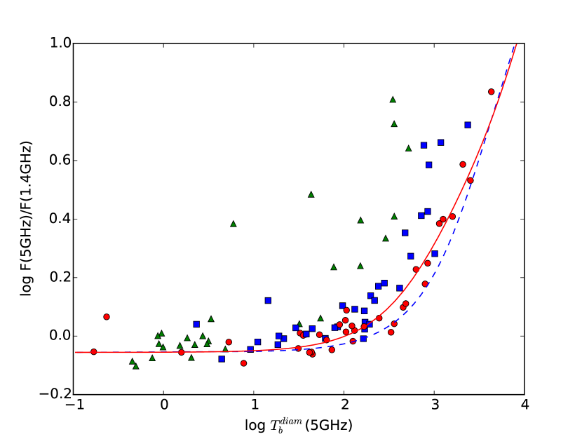
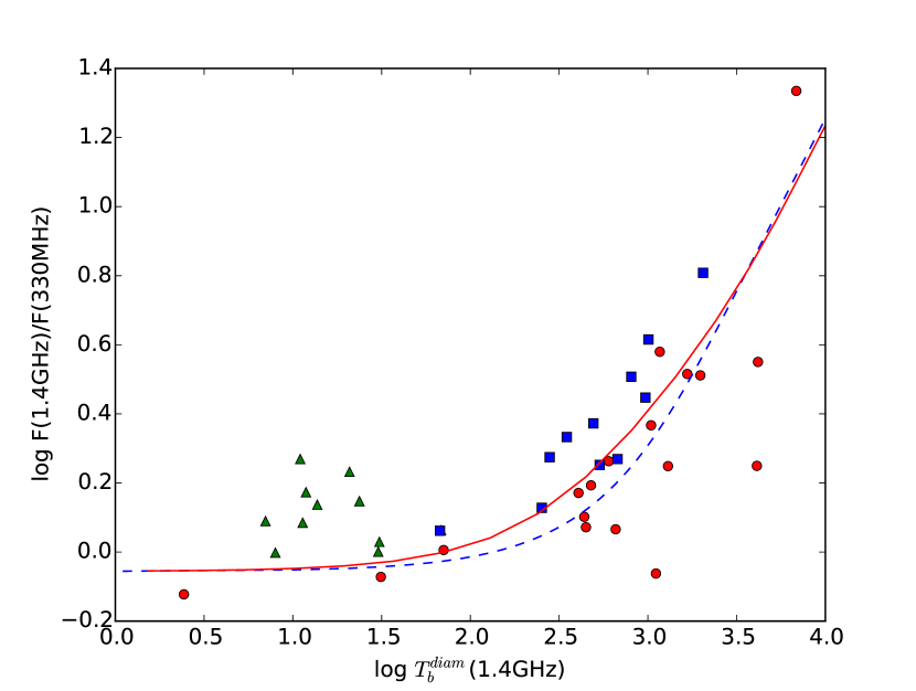
Figure 7: The observed spectral indices vs brightness temperature for PNe and model A for $T_{e}=10000\,K$ (blue line). Red curves show Model E for $a/b=3$, ${t/b}=0.1$, and $i=0^{\circ}$. PNe are marked with the symbols as in Fig. 4.

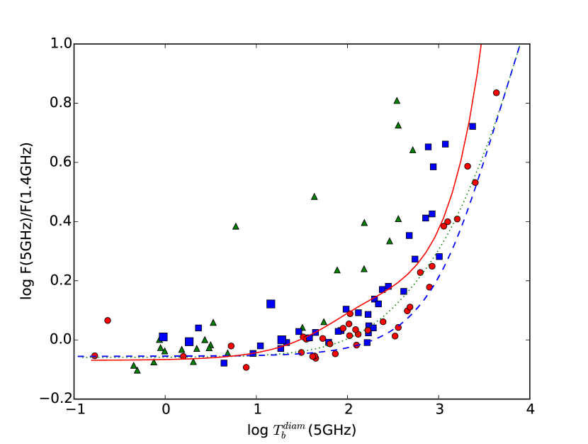
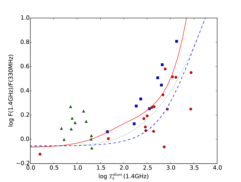
Figure 8: The observed spectral indices vs brightness temperature for PNe and model A for $T_{e}=10000\,\mathrm{K}$ (blue dashed line). Dotted curve shows model with inner region of lower temperature, while red solid curve shows model with outer region of lower temperature. PNe are marked with the symbols as in Fig. 4.

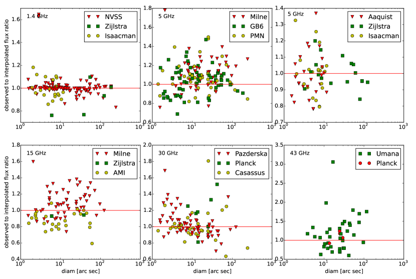
Figure 9: The ratio of the observed flux to the flux derived for model C vs PN diameter for different frequencies. For 5 GHz, single dish and interferometric surveys are shown separately.

In some cases, the excess is visible only at 5 GHz, e.g. in IC 3568, IC 5217, IC 289, or NGC 6072. Out of them, only IC 5217 shows a weak, confusing source within the primary beam of the survey of 3.5 arcmin (Gregory et al., 1996), which might be responsible for the excess of the 5 GHz/1.4 GHz ratio. However, the excess of the 5 GHz/1.4 GHz ratio does not depend on the PNe diameters, and thus cannot be affected by the presence of confusing sources in the single dish surveys. Also, 5 GHz excess was reported by Siódmiak & Tylenda (2001), who used only interferometric fluxes.

5.2 Flux evolution

One possible explanation for the 5 GHz excess could be the evolution of the radio fluxes due to nebular expansion and change of the ionizing flux from the central star. 5 GHz fluxes used in our paper are predominantly from the single dish surveys (Gregory et al., 1996; Griffith & Wright, 1993) carried out in the period $1986-1987$ and 1990. 1.4 GHz observations were taken predominately from the NRAO VLA Sky Survey (NVSS) between 1993 and 1996. Since 1.4 GHz flux should increase with respect to the 5 GHz thorough the PN evolution, the time gap between the 5 GHz surveys and NVSS should rather result in lowering the 5 GHz/1.4 GHz ratio.

Zijlstra et al. (1989) reported variability of radio flux of NGC 7027 due to expansion of the nebula (increase of $0.25\%\,yr^{-1}$) and decreasing number of ionizing photons (change of $-0.14\%\,yr^{-1}$). Such small changes would be difficult to detect with the precision of about 10% and relatively short time span between observations. However, flux evolution depends on the age of the nebula and pace of evolution of central star.

We checked the possible flux evolution using observations at the same frequency made for the same PN in different epochs, if available. We selected sources which showed more than $3\sigma$ deviation in measurements at the same frequency. In most cases, the flux measurements did not show significant changes. We rejected sources in which the possible reason for discrepancy was systemic flux error at one epoch, which did not show the expected flux changes at other frequencies and the overall flux spectrum did not show any signatures of variability, e.g. in Hu 1-2.

The variability of radio flux in IC 4997 has already been studied by Miranda & Torrelles (1998). They showed year-to-year changes of the morphology of PN IC 4997 in radio due to interaction of the collimated stellar wind with the outer shell. In the archival data, the flux at optically thin part dropped from 100 mJy around 1980 down to 50 mJy about 2000. More recent data at higher frequencies show possible increase from 80 to 110 mJy between $2001-2002$ (Casassus et al., 2007) and $2005-2007$ (Pazderska et al., 2009), respectively. However, the data are too sparse to fit the spectrum for each epoch separately.

Another case is M 2-2. This is a relatively compact PN with the diameter of only 6 arcsec. Zijlstra et al. (1989) observed higher values at 5 GHz and 15 GHz, and lower flux at 1.5 GHz than more recent observations. This would imply the lowering flux in continuum and increasing flux in optically thick part of the spectrum, in qualitative agreement with NGC 7027 (Zijlstra et al., 1989). Another possible variable is M 1-40, showing a decreasing trend over time. We would need more data to analyze the flux variability in more details. Most of PNe did not show any variability.

5.3 Radial density gradient

A spectral index of 0.6 is an indication of a strong radial density gradient ($\beta=2$). The spectral index of 0.6 should be relatively easy to confirm due to a relatively high flux at low frequencies. Phillips (2007) and Phillips (2007a) list candidates for strong density gradient. Eight of them are in common with our sample (Fig. 10). The objects were well fitted using model C except for Hu 1-2. However, the diameter of Hu 1-2 reported by Frew et al. (2016) apparently refers to the brightest, central region of the PN, while apparently much larger region of the nebula contributes to the observed radio flux (Fang et al., 2015). With larger diameter we received much better fit.

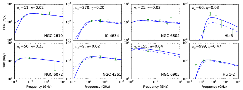
Figure 10: Spectra of PNe claimed to have strong density gradient. Solid line shows fit of model C with the parameters given in the appendix, and dashed line shows fit of model D with the parameters indicated.

Most of PNe could still be fitted with model D, but it yields worse or unrealistic fit compared to model C in about 50% of PNe. For a small value of $\eta_{B}$ model B gives artificially small densities $n_{o}$ or cannot fit the slope steeper than 0.6 in the optically thick part of the spectrum (e.g. Fig. 1, 10). Small ${\eta}_{B}$ would also result in the surface brightness quickly fading with the distance from the center of PN, and this is not confirmed in radio images (Aaquist & Kwok, 1996).

Alternatively, the observed PNe may only have thin shells. Then, the spectral index of 0.6 is observed only in a very limited range of frequencies and is difficult to confirm. However, Model D is almost equivalent to model B for large $\eta_{B}$, and cannot fit the observations of most of PNe for the same reason, described in Section 4.2.

5.4 Prolate ellipsoidal shell and temperature variations

Model E explains well the observed spectral indices of many PNe with a typical value of a/b of about 3. Alternatively, observed spectral indices could result from temperature variations. Lower temperature in the outer layer results also in lower spectral index with respect to a homogeneous model in the optically thick part of the spectrum. It would eventually produce a spectral index steeper than 2.

An upper limit from the TGSS survey indicates that some PNe show steeper spectral index than 2 in the optically thick part: NGC 6826, NGC 6543, and NGC 6818. Optically thick radio emission represents the emitting region at $\tau{\sim}2/3$, whereas optically thin emission depends on volume averaged electron temperature. Thus, at 5 GHz the excess can be interpreted as the temperature drop in the outermost regions of PN. The drop of temperature in the outer regions is not confirmed by spatially resolved spectroscopy of PNe (Sandin et al., 2008).

Model F with the temperature of 1000 K in the central region of the shell gives more flux in the optically thin region, as the emissivity of lower temperature region is higher. The optically thick spectrum is the same for the two models as radio emission originates from the outermost region of the shell. The region with lower temperature was indicated by Tsamis et al. (2004) and is one of the alternative explanations for the abundance discrepancy problem in PNe. García-Rojas et al. (2017) showed that emission originating from optical recombination lines is more centrally concentrated than emission from collisionally excited lines.

5.5 Low surface brightness PNe

Unexpectedly, a group of PNe with low $T_{b}^{diam}$ shows non-negligible optical thickness at lowest frequencies (Figs. 7,8). Model C gives $\eta>0.9$, which indicates that a small part of the projected area of the PN with high $EM$ contribute most of the radio flux. However, NVSS and other catalogs give the radii comparable to that seen in optical. This suggests that they form a cylindrical shell observed along its axis, which causes strong limb brightening, or contain a compact component, which contribution in flux is comparable to the rest of PN. Relatively low $M_{i}$ indicate that these structures comprise only part of the nebular ionized mass.

Figure 6 shows, that for low surface brightness PNe $S_{0}(\mathrm{H}\alpha)<-2$ only those with large $\eta$ parameter are observed. According to Aaquist & Kwok (1996), morphology of PNe does not change between low and high surface brightness PNe. This indicates, that low surface brightness PNe are detected only when they contain a small region with high column density.

This group contains bipolar or quadrupolar PNe NGC 650-51, NGC 4361, NGC 6302, or M 1-75. Also, three PNe classified as round, NGC 2610, Abell 53, and NGC 6842, belong to this group, indicating, that their spatial structure is more complex than spherical.

6 Summary

In conclusion, we confirm that homogeneous models cannot fit the observed radio spectra and brightness temperatures of most of PNe. We do not find an evidence for a strong radial density gradient in PNe. We found a sample of PNe showing two component spectra, but they cannot account for the observed 5 GHz to 1.4 GHz indices. A model of prolate ellipsoidal shell or temperature variations explain very well the observed spectral indices with except of low surface brightness PNe. Part of low surface brightness PNe are only observed in radio due to their specific morphology. Further observations at low frequencies having better sensitivity and resolution, e.g. Low Frequency Array (van Haarlem et al., 2013) will better constrain the spectral index in optically thick part of the spectra and geometry of PNe.

Appendix A Emission measures and $\eta$ values derived for Model C

Table 2: Modeled temperatures and emission measures.

Name	RA (J2000)	DEC (J2000)	$EM[cm^{-6}pc]$	error EM	$\eta$	error $\eta$	$\tau_{5GHz}$	$T_{b}^{spec}$	$T_{b}^{diam}$
NGC 40	00 13 01.010	+72 31 19.09	3.476E+5	6.943E+4	0.7283	0.0563	0.00338	37.158	18.260
Hu 1-1	00 28 15.435	+55 57 54.48	4.206E+5	3.375E+5	0.0000		0.00360	43.508	45.537
NGC 246	00 47 03.338	-11 52 18.94	2.174E+3	2.008E+5	0.0000		0.00001	0.205	0.214
NGC 650-51	01 42 19.69	+51 34 31.7	2.315E+5	5.031E+4	0.9907	0.0019	0.00234	24.995	0.485
IC 1747	01 57 35.734	+63 19 18.33	4.005E+5	1.284E+5	0.5174	0.2177	0.00437	44.054	33.766
IC 289	03 10 19.30	+61 19 01.0	8.199E+4	9.264E+4	0.6561	0.4832	0.00050	7.792	4.645
M 1-4	03 41 43.439	+52 16 59.85	3.046E+6	1.756E+6	0.0000		0.02419	305.881	320.152
IC 2003	03 56 22.027	+33 52 29.27	4.048E+5	1.118E+6	0.0000		0.00347	41.869	43.822
NGC 1501	04 06 59.39	+60 55 14.4	3.304E+5	5.757E+4	0.9234	0.0126	0.00210	31.671	4.885
NGC 1514	04 09 16.985	+30 46 33.47	7.418E+4	3.716E+4	0.9669	0.0163	0.00074	7.989	0.544
M 2-2	04 13 15.043	+56 56 58.12	8.573E+5	8.093E+5	0.0000		0.00726	88.263	92.380
NGC 1535	04 14 15.765	-12 44 21.90	1.927E+5	3.384E+4	0.7032	0.0604	0.00173	20.182	10.678
IC 418	05 27 28.203	-12 41 50.26	8.455E+6	1.807E+6	0.3525	0.2460	0.09743	900.472	825.399
NGC 2022	05 42 06.20	+09 05 10.3	1.671E+5	5.508E+4	0.6989	0.1180	0.00108	16.099	8.620
M 1-5	05 46 50.01	+24 22 02.8	7.838E+6	1.145E+6	0.3964	0.1215	0.09837	852.525	752.131
IC 2149	05 56 23.901	+46 06 17.19	1.041E+6	1.975E+5	0.1948	0.4433	0.01107	113.344	114.128
IC 2165	06 21 42.775	-12 59 13.96	4.652E+6	1.113E+6	0.7950	0.0501	0.03305	451.917	174.056
J 900	06 25 57.237	+17 47 27.53	1.973E+6	8.423E+5	0.6452	0.1800	0.01690	202.745	123.857
M 1-6	06 35 45.126	-00 05 37.36	1.108E+7	9.299E+5	0.6784	0.0240	0.11939	1147.872	648.450
NGC 2371	07 25 34.68	+29 29 26.4	1.374E+5	4.887E+4	0.9216	0.0285	0.00096	13.496	2.127
NGC 2392	07 29 10.765	+20 54 42.48	2.913E+5	1.030E+5	0.8226	0.0678	0.00174	27.486	9.301
NGC 2438	07 41 50.51	-14 44 07.7	1.667E+6	2.008E+6	0.9975	0.0028	0.01643	177.596	0.926
NGC 2440	07 41 54.91	-18 12 29.7	5.303E+5	2.003E+5	0.8018	0.0829	0.00373	52.150	19.491
Hen 2-9	08 28 27.924	-39 23 39.92	4.864E+6	4.600E+5	0.4135	0.0560	0.05240	520.713	451.809
NGC 2610	08 33 23.40	-16 08 57.5	1.042E+6	2.562E+5	0.9955	0.0010	0.00530	94.097	0.885
Hen 2-11	08 37 08.10	-39 25 07.0	1.720E+5	2.866E+4	0.9189	0.0135	0.00185	18.883	3.074
Hen 2-15	08 53 30.91	-40 03 42.3	2.074E+5	1.167E+5	0.7399	0.1666	0.00152	20.618	9.767
NGC 2867	09 21 25.38	-58 18 40.9	1.396E+6	2.150E+5	0.5991	0.0750	0.01265	145.869	97.873
IC 2501	09 38 47.146	-60 05 30.52	5.510E+6	6.918E+5	0.7746	0.0284	0.06262	594.869	249.031
NGC 3132	10 07 01.764	-40 26 11.12	2.046E+5	8.553E+4	0.9436	0.0232	0.00226	22.607	2.595
Hen 2-47	10 23 09.14	-60 32 42.3	6.968E+6	5.956E+5	0.5406	0.0459	0.07522	739.082	547.105
NGC 3242	10 24 46.107	-18 38 32.64	5.172E+5	5.306E+4	0.6945	0.0250	0.00486	54.735	29.656
IC 2621	11 00 19.99	-65 14 57.8	2.760E+7	1.244E+6	0.7107	0.0143	0.21028	2503.267	1296.595
NGC 3587	11 14 47.701	+55 01 08.72	1.550E+3	8.467E+4	0.0000		0.00002	0.166	0.174
NGC 3918	11 50 17.77	-57 10 56.4	3.916E+6	4.138E+5	0.7457	0.0292	0.03210	394.906	183.515
NGC 4361	12 24 30.76	-18 47 05.4	1.884E+6	4.679E+5	0.9974	0.0005	0.00835	163.881	0.876
IC 3568	12 33 06.871	+82 33 48.95	6.186E+5	1.398E+5	0.8415	0.0380	0.00649	67.305	20.559
NGC 5307	13 51 03.322	-51 12 20.77	3.122E+5	1.570E+5	0.5694	0.2821	0.00251	31.779	22.478
NGC 5315	13 53 57.00	-66 30 50.7	8.513E+6	7.811E+5	0.8083	0.0172	0.10529	919.434	333.545
Hen 2-113	14 59 53.476	-54 18 07.42	5.718E+7	2.292E+7	0.0000		0.61588	4690.332	4910.109
Hen 2-142	15 59 57.63	-55 55 33.0	9.975E+6	1.195E+6	0.7862	0.0258	0.10745	1039.136	415.443
IC 4593	16 11 44.544	+12 04 17.06	1.578E+6	5.534E+5	0.9192	0.0255	0.02040	179.739	29.183
NGC 6072	16 12 58.40	-36 13 47.0	6.337E+4	3.877E+4	0.8552	0.0945	0.00059	6.701	1.884
NGC 6153	16 31 30.626	-40 15 12.31	1.603E+6	3.786E+5	0.7782	0.0563	0.01541	169.767	70.093
NGC 6210	16 44 29.491	+23 47 59.68	9.176E+5	6.085E+5	0.0000		0.01057	102.019	106.778
IC 4634	17 01 33.57	-21 49 33.3	1.171E+6	1.229E+5	0.7378	0.0286	0.01331	129.607	61.816
NGC 6302	17 13 44.339	-37 06 10.95	9.779E+6	2.545E+6	0.9678	0.0073	0.05513	884.954	58.724
NGC 6309	17 14 04.299	-12 54 35.74	3.615E+5	8.531E+4	0.4552	0.1719	0.00339	38.289	31.772
H 1-13	17 28 27.503	-35 07 31.58	3.514E+6	1.464E+6	0.5394	0.2006	0.03785	378.898	281.174
NGC 6369	17 29 20.45	-23 45 34.8	2.369E+6	5.004E+5	0.5832	0.1157	0.01942	240.382	166.032
Hb 4	17 41 52.80	-24 42 08.7	3.319E+6	4.091E+5	0.7387	0.0346	0.01942	353.915	168.292
Hb 5	17 47 56.20	-29 59 39.6	2.668E+7	6.677E+6	0.9933	0.0007	0.03396	2404.431	33.666
NGC 6445	17 49 15.21	-20 00 34.5	1.858E+6	6.527E+5	0.9934	0.0022	0.01665	193.196	2.675
NGC 6543	17 58 33.423	+66 37 59.52	1.112E+6	7.615E+4	0.5645	0.0379	0.01630	130.998	93.416
NGC 6537	18 05 13.104	-19 50 34.88	1.126E+7	9.717E+5	0.8038	0.0164	0.06789	1030.472	381.725
M 1-40	18 08 25.989	-22 16 52.93	3.543E+6	2.567E+6	0.7090	0.2182	0.02936	358.767	186.746
M 1-41	18 09 30.10	-24 12 26.0	3.087E+6	2.685E+6	0.9940	0.0042	0.03042	326.550	4.080
NGC 6572	18 12 06.365	+06 51 13.01	1.532E+7	1.172E+6	0.8508	0.0111	0.16286	1547.986	447.504
SwSt 1	18 16 12.268	-30 52 08.01	6.488E+7	6.079E+6	0.9599	0.0029	0.69886	5129.055	422.482
NGC 6578	18 16 16.517	-20 27 02.67	9.625E+5	8.108E+5	0.5474	0.5162	0.01037	105.203	77.117
Cn 3-1	18 17 34.113	+10 09 03.46	7.673E+6	2.850E+6	0.8544	0.0512	0.03022	639.986	180.845
NGC 6629	18 25 42.458	-23 12 10.23	1.613E+6	7.764E+5	0.7826	0.1069	0.02117	184.324	74.756
M 2-43	18 26 40.05	-02 42 57.3	1.146E+8	1.381E+7	0.5506	0.0539	1.23460	7232.283	5277.104
M 1-51	18 33 29.05	-11 07 26.5	3.911E+6	1.599E+6	0.7893	0.0858	0.04212	420.741	166.031
M 1-59	18 43 20.20	-09 04 49.1	6.214E+6	1.119E+6	0.8287	0.0263	0.06693	660.372	216.476
M 1-61	18 45 55.12	-14 27 37.9	3.085E+7	2.752E+6	0.3319	0.0728	0.33230	2883.860	2686.219
Hu 2-1	18 49 47.567	+20 50 39.45	1.942E+7	1.565E+6	0.9028	0.0051	0.22686	1948.460	377.028
NGC 6720	18 53 35.079	+33 01 45.03	1.438E+5	4.327E+4	0.8529	0.0474	0.00138	15.336	4.375
K 3-17	18 56 18.164	+07 07 25.88	3.817E+6	9.507E+5	0.8458	0.0379	0.04111	410.849	122.363
M 1-66	18 58 26.24	-01 03 45.6	7.136E+6	2.707E+6	0.5779	0.1432	0.07687	754.659	526.094
NGC 6741	19 02 37.10	-00 26 56.7	1.034E+7	2.005E+6	0.8794	0.0179	0.08388	1013.822	240.583
Abell 53	19 06 45.910	+06 23 52.47	1.868E+7	3.379E+6	0.9986	0.0001	0.15997	1788.741	5.234
Hen 2-430	19 14 04.13	+17 31 33.1	1.581E+7	7.609E+5	0.9084	0.0024	0.17035	1597.668	292.355
NGC 6781	19 18 28.085	+06 32 19.29	1.358E+4	4.336E+5	0.0000		0.00015	1.502	1.572
NGC 6790	19 22 56.966	+01 30 46.46	6.330E+7	3.213E+6	0.8698	0.0055	0.50259	5056.511	1288.885
Vy 2-2	19 24 22.223	+09 53 56.29	6.476E+8	8.626E+7	0.9802	0.0021	6.97563	10190.46	419.323
K 3-35	19 27 44.02	+21 30 03.4	2.712E+7	4.541E+6	0.9629	0.0036	0.29215	2584.072	196.957
PB 10	19 28 14.487	+12 19 37.11	1.683E+6	5.816E+5	0.8975	0.0336	0.01812	183.209	37.305
NGC 6803	19 31 16.47	+10 03 21.7	7.843E+6	1.006E+6	0.8254	0.0170	0.09164	840.595	280.474
NGC 6804	19 31 35.14	+09 13 31.4	3.116E+6	2.165E+6	0.9954	0.0029	0.02929	325.928	3.138
BD+30 3639	19 34 45.233	+30 30 58.94	2.083E+7	1.113E+6	0.6156	0.0230	0.22435	2049.857	1332.475
M 1-71	19 36 26.92	+19 42 24.1	1.768E+7	6.701E+5	0.7992	0.0066	0.19561	1776.664	671.951
M 1-73	19 41 09.29	+14 56 58.8	5.391E+5	9.091E+5	0.1400		0.00581	59.059	60.604
NGC 6818	19 43 58.022	-14 09 13.44	4.079E+5	5.174E+4	0.4568	0.0841	0.00324	41.388	34.278
NGC 6826	19 44 48.150	+50 31 30.26	7.624E+5	2.299E+5	0.6526	0.1269	0.00724	80.840	48.581
Hen 2-447	19 45 22.16	+21 20 03.9	1.886E+7	2.082E+6	0.6390	0.0360	0.20315	1875.197	1161.339
NGC 6842	19 55 02.1	+29 17 22	5.860E+5	1.929E+5	0.9915	0.0026	0.00310	53.516	0.953
Hen 1-4	19 59 18.014	+31 54 39.14	9.712E+6	1.249E+7	0.9981	0.0012	0.10743	1018.633	4.074
K 3-52	20 03 11.44	+30 32 34.1	3.597E+7	3.695E+6	0.8536	0.0108	0.38751	3276.799	930.736
M 1-75	20 04 44.1	+31 27 28	3.408E+5	3.187E+4	0.9782	0.0019	0.00367	37.378	1.690
K 3-55	20 06 56.250	+32 16 36.80	1.463E+6	4.549E+5	0.7405	0.0862	0.01576	159.488	75.407
NGC 6884	20 10 23.66	+46 27 39.8	3.662E+6	5.046E+5	0.6440	0.0526	0.03893	393.269	240.900
NGC 6881	20 10 52.45	+37 24 42.4	8.812E+6	2.081E+6	0.9300	0.0130	0.08176	894.926	126.555
NGC 6886	20 12 42.83	+19 59 22.6	4.327E+6	1.933E+6	0.8147	0.0783	0.03364	430.087	151.363
K 3-57	20 12 47.725	+34 20 32.79	7.122E+5	1.228E+6	0.0000		0.00767	77.950	81.586
Hen 2-459	20 13 57.89	+29 33 55.9	4.854E+7	7.524E+6	0.8936	0.0120	0.52288	4153.345	876.039
NGC 6891	20 15 08.838	+12 42 15.63	2.839E+6	8.101E+5	0.9168	0.0213	0.03058	307.163	51.258
NGC 6894	20 16 23.965	+30 33 53.17	3.999E+5	2.284E+5	0.9844	0.0087	0.00431	43.846	1.423
IC 4997	20 20 08.742	+16 43 53.71	3.976E+7	9.787E+6	0.7952	0.0417	0.18786	3219.897	1238.914
M 3-35	20 21 03.77	+32 29 24.0	4.596E+7	3.791E+6	0.9272	0.0044	0.49506	3982.741	585.173
NGC 6905	20 22 22.991	+20 06 16.25	2.252E+6	1.514E+6	0.9933	0.0041	0.01928	231.096	3.226
NGC 7008	21 00 32.7	+54 32 39	1.096E+5	2.465E+4	0.9138	0.0195	0.00118	12.038	2.078
NGC 7009	21 04 10.877	-11 21 48.26	8.012E+5	5.440E+4	0.3776	0.0552	0.00911	88.827	79.713
NGC 7026	21 06 18.237	+47 51 07.15	9.590E+5	7.862E+4	0.8750	0.0075	0.01204	108.877	26.709
NGC 7027	21 07 01.8	+42 14 10	5.450E+7	9.574E+6	0.6965	0.0630	0.45157	4505.795	2428.366
NGC 7048	21 14 15.25	+46 17 16.1	1.885E+5	1.909E+5	0.9820	0.0174	0.00153	19.248	0.719
K 3-62	21 31 50.18	+52 33 51.6	9.779E+6	1.930E+6	0.7430	0.0418	0.10534	1019.792	478.198
IC 5117	21 32 30.97	+44 35 47.5	6.225E+7	2.563E+6	0.7291	0.0092	0.56422	5001.907	2452.423
Hu 1-2	21 33 08.328	+39 38 09.72	3.021E+6	3.404E+6	0.0000		0.03529	332.913	348.447
Bl 2-1	22 20 16.63	+58 14 16.6	1.637E+7	2.118E+6	0.4362	0.0782	0.17631	1648.746	1397.387
IC 5217	22 23 55.73	+50 58 00.5	1.504E+6	9.728E+5	0.7386	0.1812	0.01363	157.056	74.700
Me 2-2	22 31 43.683	+47 48 03.91	2.123E+7	1.951E+6	0.7895	0.0127	0.21177	2061.190	812.550
NGC 7354	22 40 19.83	+61 17 08.7	7.675E+5	1.342E+5	0.7503	0.0446	0.00650	79.049	36.155
NGC 7662	23 25 53.6	+42 32 06	8.681E+5	1.240E+5	0.6821	0.0508	0.00689	87.918	49.206

Appendix B Spectra of individual PNe

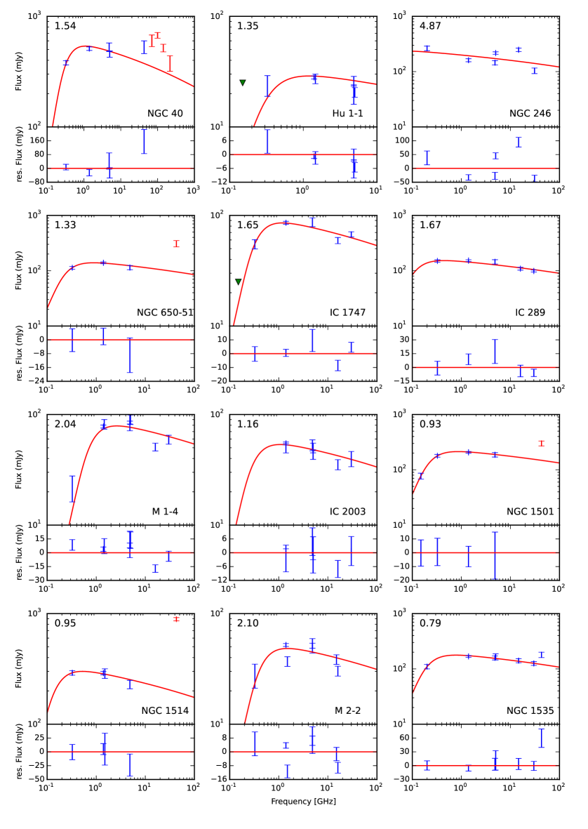
Figure 11: Radio spectra and best model fits for PNe radio spectra. Triangles set an upper limit for the TGSS survey, if it is lower than the next data point. Red errorbars mark data not used in the fit.

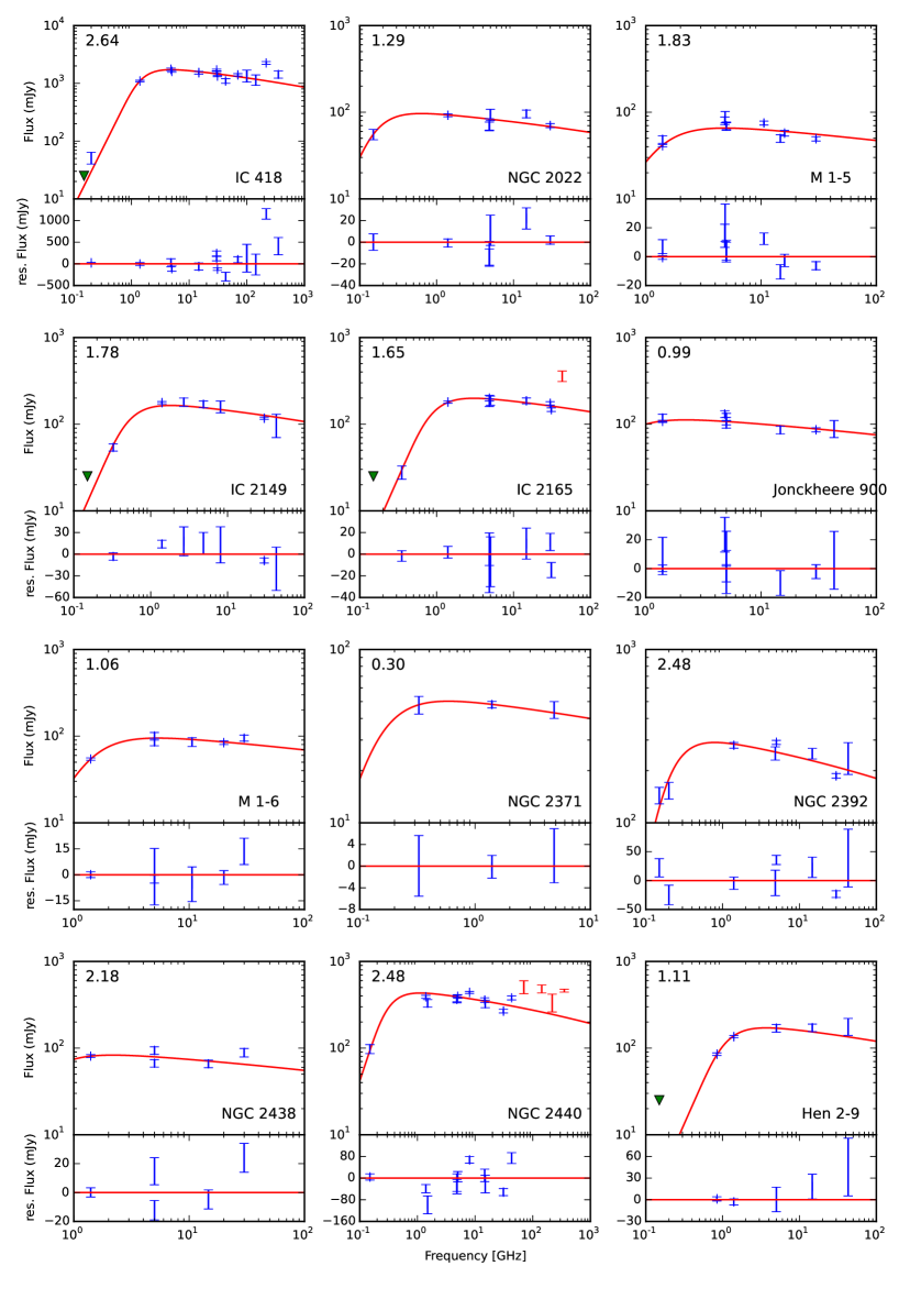
Figure 12: Radio spectra and best model fits for PNe radio spectra. Triangles set an upper limit for the TGSS survey, if it is lower than the next data point. Red errorbars mark data not used in the fit.

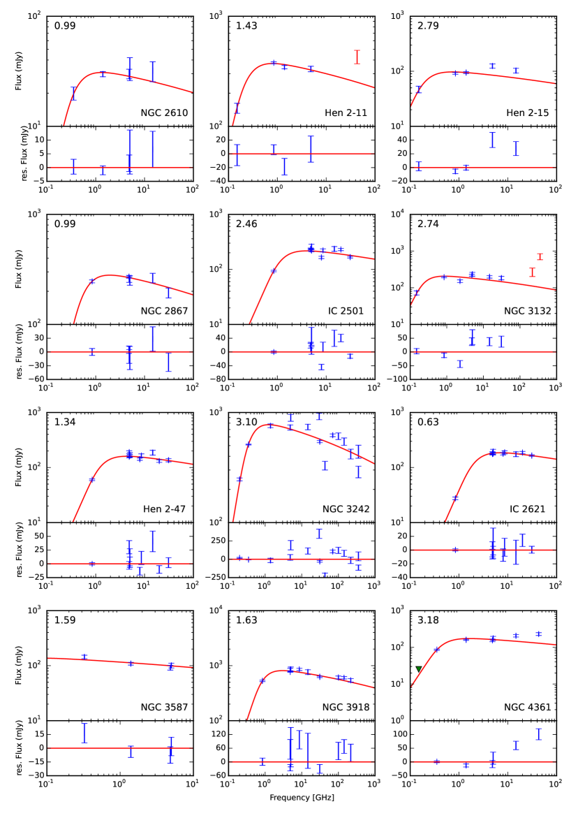
Figure 13: Radio spectra and best model fits for PNe radio spectra. Triangles set an upper limit for the TGSS survey, if it is lower than the next data point. Red errorbars mark data not used in the fit.

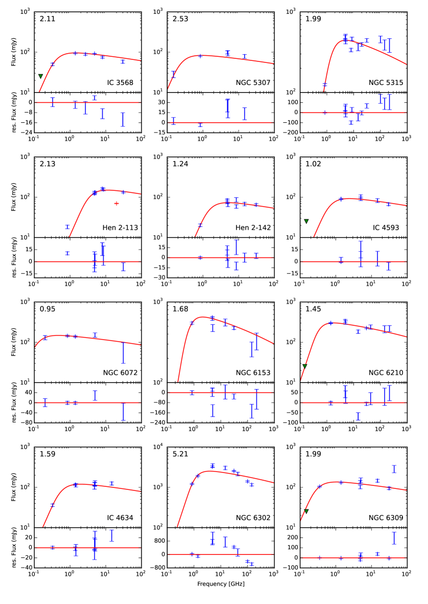
Figure 14: Radio spectra and best model fits for PNe radio spectra. Triangles set an upper limit for the TGSS survey, if it is lower than the next data point. Red errorbars mark data not used in the fit.

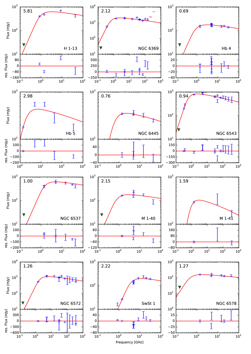
Figure 15: Radio spectra and best model fits for PNe radio spectra. Triangles set an upper limit for the TGSS survey, if it is lower than the next data point. Red errorbars mark data not used in the fit.

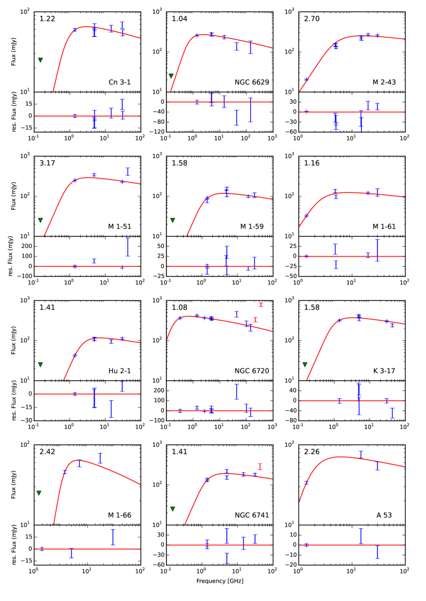
Figure 16: Radio spectra and best model fits for PNe radio spectra. Triangles set an upper limit for the TGSS survey, if it is lower than the next data point. Red errorbars mark data not used in the fit.

Figure 17: Radio spectra and best model fits for PNe radio spectra. Triangles set an upper limit for the TGSS survey, if it is lower than the next data point. Red errorbars mark data not used in the fit.

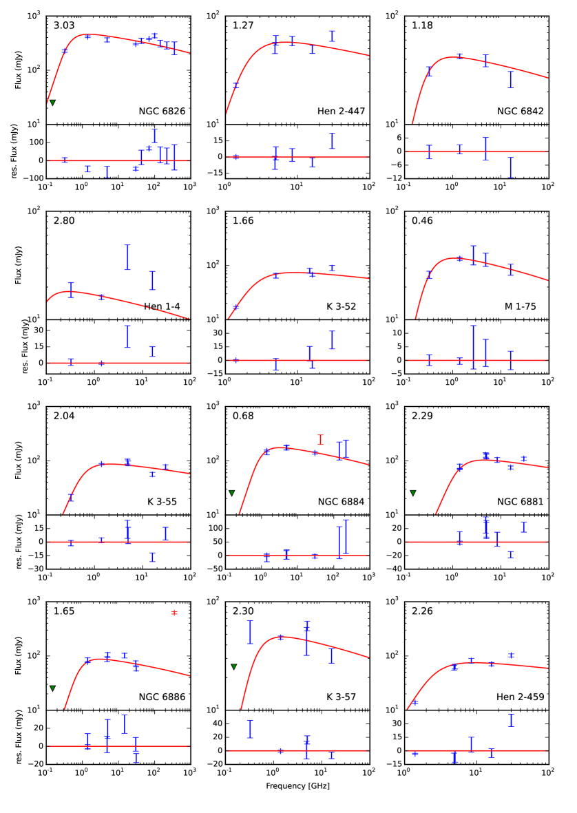
Figure 18: Radio spectra and best model fits for PNe radio spectra. Triangles set an upper limit for the TGSS survey, if it is lower than the next data point. Red errorbars mark data not used in the fit.

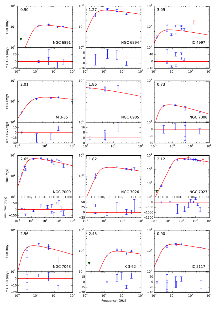
Figure 19: Radio spectra and best model fits for PNe radio spectra. Triangles set an upper limit for the TGSS survey, if it is lower than the next data point. Red errorbars mark data not used in the fit.

Figure 20: Radio spectra and best model fits for PNe radio spectra. Triangles set an upper limit for the TGSS survey, if it is lower than the next data point. Red errorbars mark data not used in the fit.

References

- Aaquist & Kwok (1990) Aaquist, O. B. & Kwok, S. 1990, A&AS, 84, 229
- Aaquist & Kwok (1996) Aaquist, O. B. & Kwok, S. 1996, ApJ, 462, 813
- Cahn et al. (1992) Cahn, J. H., Kaler, J. B. & Stanghellini, L. 1992, A&AS, 94, 399
- Casassus et al. (2007) Casassus, S., Nyman, L.-øA., Dickinson, C., Pearson, T. J. 2007, MNRAS, 382, 1607
- Chhetri et al. (2015) Chhetri, R., Ekers, R. D., Kimball, A., et al. 2007, MNRAS, 382, 1607
- Condon et al. (1998) Condon, J. J., Cotton, W. D., Greisen, E. W., et al. 1998, AJ, 115, 1693
- De Breuck et al. (2002) De Breuck, C., Tang, Y., de Bruyn, A. G. Röttgering, H. & van Breugel, W. 2002, A&A, 394, 59
- Di Francesco et al. (2008) Di Francesco, J., Johnstone, D., Kirk, H., MacKenzie, T. & Ledwosinska, E. 2008, ApJS, 175, 277
- Douglas et al. (1996) Douglas, J. N., Bash, F. N., Bozyan, F. A., Torrence, G. W. & Wolfe, C. 1996, AJ, 111, 1945
- Fang et al. (2015) Fang, X., Guerrero, M. A., Miranda, L. F., et al. 2015, MNRAS, 452, 2445
- Frew et al. (2016) Frew, D. J., Parker, Q. A., Bojičić, I. S. 2016, MNRAS, 455, 1459
- García-Rojas et al. (2017) García-Rojas, J., et al. 2017, IAUS, 323, 65
- Gregory et al. (1996) Gregory, P. C., Scott, W. K., Douglas, K. & Condon, J. J. 1996, ApJS, 103, 427
- Griffith & Wright (1993) Griffith, M. R., Wright, A. E. 1993, AJ, 105, 1666
- Gruenwald & Aleman (2007) Gruenwald, R., Aleman, A. 2007, A&A, 461, 1019
- Hurley-Walker et al. (2017) Hurley-Walker, N., Callingham, J. R., Hancock, P. J., et al. 2017, MNRAS, 464, 1146
- Intema et al. (2017) Intema, H. T., Jagannathan, P., Mooley, K. P. & Frail, D. A. 2017, A&A, 598A, 78
- Isaacman (1984) Isaacman, R. 1984, MNRAS, 208, 399
- Marigo (2001) Marigo, P. 2001, A&A, 370, 194
- Masson (1990) Masson, C. R. 1990, ApJ, 348, 580
- Mauch et al. (2003) Mauch, T., Murphy, T., Buttery, H. J., et al. 2003, MNRAS, 342, 1117
- McConnell (2012) McConnell, D., Sadler, E. M., Murphy, T., Ekers, R. D. 2012, MNRAS, 422, 1527
- Milne & Aller (1975) Milne, D. K. & Aller, L. H. 1975, A&A, 38, 183
- Milne & Aller (1982) Milne, D. K. & Aller, L. H. 1982, A&AS, 50, 209
- Miranda & Torrelles (1998) Miranda, L. F.; Torrelles, J. M. 1998, ApJ, 496, 274
- Murphy et al. (2007) Murphy, T., Mauch, T., Green, A. et al. 2007, MNRAS, 382, 382
- Murphy et al. (2010) Murphy, T., Sadler, E. M., Ekers, R. D. et al. 2010, MNRAS, 402, 2403
- O’Dell et al. (2013) O’Dell, C. R., Ferland, G. J., Henney, W. J., Peimbert, M. 2013, AJ, 145, 170O
- Olnon (1975) Olnon, F. M. 1975, A&A, 39, 217
- Pazderska et al. (2009) Pazderska, B. M., Gawroński, M. P., Feiler, R., et al. 2009, A&A, 498, 463
- Perrott et al. (2015) Perrott, Y. C., Scaife, A. M. M., Green, D. A., et al. 2015, MNRAS, 453, 1396
- Phillips (2007) Phillips, J. P. 2007, MNRAS, 378, 231
- Phillips (2007a) Phillips, J. P. 2007, RMxAA, 43, 303
- Planck Collaboration (2016) Planck Collaboration XXVI. 2016, A&A, 594, A26
- Rengelink et al. (1997) Rengelink, R. B., Tang, Y., de Bruyn, A. G., et al. 1997, A&AS, 124, 259
- Sahai et al. (2011) Sahai, R., Morris, M. R., Villar, G. G. 2011, AJ, 141, 134S
- Sandin et al. (2008) Sandin, R., et al. 2008, A&A, 486, 545
- Siódmiak & Tylenda (2001) Siódmiak, N., Tylenda, R. 2001, A&A, 373, 1032
- Taylor et al. (1996) Taylor, A. R., Goss, W. M., Coleman, P. H., van Leeuwen, J. & Wallace, B. J. 1996, ApJS, 107, 239
- Tsamis et al. (2004) Tsamis, Y. G., Barlow, M. J., Liu, X. W., Storey, P. J., Danziger, I. J. 2004, MNRAS, 353, 953
- Umana et al. (2008) Umana, G., Leto, P., Trigilio, C., et al. 2008, A&A, 482, 529
- van Haarlem et al. (2013) van Haarlem, M. P., Wise, M. W., Gunst, A. W., et al. 2013, A&A, 556A, 2
- van Hoof et al. (2014) van Hoof, P. A. M., Williams, R. J. R., Volk, K., et al. 2014, MNRAS, 444, 420
- Wenger et al. (2000) Wenger, M., Ochsenbein, F., Egret, D., et al. 2000, A&AS, 143, 9W
- Zijlstra et al. (1989) Zijlstra, A. A., Pottasch, S. R., Bignell, C., et al. 1989, A&AS, 79, 329
- Zijlstra et al. (1989) Zijlstra, A. A., van Hoof, P. A. M., Perley, R. A. 2008, ApJ, 681, 1296