Long-time oscillatory energy conservation of total energy-preserving methods for highly oscillatory
Hamiltonian systems

Abstract

For an integrator when applied to a highly oscillatory system, the near conservation of the oscillatory energy over long times is an important aspect. In this paper, we study the long-time near conservation of oscillatory energy for the adopted average vector field (AAVF) method when applied to highly oscillatory Hamiltonian systems. This AAVF method is an extension of the average vector field method and preserves the total energy of highly oscillatory Hamiltonian systems exactly. This paper is devoted to analysing another important property of AAVF method, i.e., the near conservation of its oscillatory energy in a long term. The long-time oscillatory energy conservation is obtained via constructing a modulated Fourier expansion of the AAVF method and deriving an almost invariant of the expansion. A similar result of the method in the multi-frequency case is also presented in this paper.

Keywords: highly oscillatory Hamiltonian systems, modulated Fourier expansion, AAVF method, energy-preserving methods, long-time oscillatory energy conservation.

MSC (2000): 65P10, 65L05

1 Introduction

This paper is concerned with the long-time oscillatory energy behaviour of energy-preserving methods for the highly oscillatory Hamiltonian system

$$\left\{\begin{aligned} &\dot{q}=\nabla_{p}H(q,p),\qquad\ \ q(0)=q_{0},\\ &\dot{p}=-\nabla_{q}H(q,p),\qquad p(0)=p_{0},\end{aligned}\right.$$ (1)

where the Hamiltonian function is given by

$$H(q,p)=\frac{1}{2}\big{(}\left\|p\right\|^{2}+\left\|\Omega q\right\|^{2}\big{)}+U(q).$$ (2)

Here $U(q)$ is a real-valued function. According to the partition of the square matrix

$$\Omega=\left(\begin{array}[]{cc}0_{d_{1}\times d_{1}}&0_{d_{2}\times d_{2}}\\ 0_{d_{1}\times d_{1}}&\omega I_{d_{2}\times d_{2}}\\ \end{array}\right)$$

with a large positive parameter $\omega$, the vectors $p=(p_{1},p_{2})\in\mathbb{R}^{d_{1}}\times\mathbb{R}^{d_{2}}$ and $q=(q_{1},q_{2})\in\mathbb{R}^{d_{1}}\times\mathbb{R}^{d_{2}}$ are partitioned accordingly. As is known, the oscillatory energy of the system (1) is

$$I(q,p)=\frac{1}{2}p_{2}^{\intercal}p_{2}+\frac{1}{2}\omega^{2}q_{2}^{\intercal}q_{2}$$ (3)

and it is nearly conserved over long times along the solution of (1) (see [16]). Our attention of this paper will particularly focus on the near conservation of the oscillatory energy (3) for energy-preserving methods over long-time intervals.

In order to preserve the total energy of Hamiltonian systems exactly by numerical methods, energy-preserving (EP) methods have been proposed and researched. In the recent decades, various kinds of EP methods have been derived, such as the average vector field (AVF) method [4, 5, 29], discrete gradient methods [24, 25], the energy-preserving collocation methods [7, 12], Hamiltonian Boundary Value Methods [2, 3], energy-preserving exponentially-fitted methods [27, 28], and time finite elements methods [1, 20, 35]. By taking advantage the frequency matrix of second-order highly oscillatory systems, a novel adopted AVF (AAVF) method has been formulated and studied in [34, 39] for the highly oscillatory Hamiltonian system (2). It has been proved in [34, 39] that this AAVF method exactly preserves the total energy (2) and it reduces to the AVF method when the frequency matrix vanishes. However, most existing publications dealing with EP methods focus on the formulation of the methods and the analysis of the EP property. It seems that the long-time behaviour of AAVF method concerning other structure-preserving aspects has never been studied in the literature, such as the long-time numerical conservation of oscillatory energies. As is well known that an important property of highly oscillatory systems is the near conservation of the oscillatory energy over long times.

On the other hand, in the recent two decades, modulated Fourier expansion has been presented and developed as an important mathematical tool in the study of the long-time behaviour for numerical methods/differential equations (see, e.g. [6, 10, 15]). It was firstly given in [14] and has been used in the long-time analysis for various numerical methods, such as for the Störmer–Verlet method in [13], for trigonometric integrators in [6, 16], for an implicit-explicit method in [26, 31], for heterogeneous multiscale methods in [30] and for splitting methods in [9, 11]. However, it is noted that, until now, the technique of modulated Fourier expansions has not been well applied to the long-term analysis for any energy-preserving method in the literature.

Based on the facts stated above, the main contribution of this paper is to analyse the long-time oscillatory energy conservation for the AAVF method. To this end, the technique of modulated Fourier expansions with some adaptations will be used in the analysis. To our knowledge, this paper is the first one that rigorously studies the remarkable long-time oscillatory energy conservation of EP methods on highly oscillatory Hamiltonian systems by using modulated Fourier expansions.

The rest of this paper is organised as follows. We first present the scheme of AAVF method and carry out an illustrative numerical experiment in Section 2. Section 3 derives the modulated Fourier expansion of the AAVF method and analyse the bounds of the modulated Fourier functions. In Section 4, we show an almost invariant of the modulation system and then the main result concerning the long-time oscillatory energy conservation of AAVF method is derived. Section 5 extends the analysis to multi-frequency case and studies the long-time conservation of AAVF method when applied to multi-frequency highly oscillatory Hamiltonian systems. The last section includes the concluding remarks of this paper.

2 The AAVF method and illustrative numerical experiments

The highly oscillatory Hamiltonian system (2) can be rewritten as a system of second-order differential equations

$$q^{\prime\prime}(t)+\Omega^{2}q(t)=f(q(t)),\qquad q(0)=q_{0},\ \ q^{\prime}(0)=p_{0},$$ (4)

where $f$ is the negative gradient of the real-valued function $U(q)$. For effectively integrating this second-order highly oscillatory system, a novel kind of EP methods was derived in [34, 39].

Definition 2.1

(See [34, 39]) The adapted AVF (AAVF) method for solving (4) is defined by

$$\left\{\begin{aligned} q_{n+1}&=\phi_{0}(V)q_{n}+h\phi_{1}(V)p_{n}+h^{2}\phi_{2}(V)\displaystyle\int_{0}^{1}f((1-\tau)q_{n}+\tau q_{n+1})d\tau,\\ p_{n+1}&=-h\Omega^{2}\phi_{1}(V)q_{n}+\phi_{0}(V)p_{n}+h\phi_{1}(V)\displaystyle\int_{0}^{1}f((1-\tau)q_{n}+\tau q_{n+1})d\tau,\end{aligned}\right.$$ (5)

where $h$ is the stepsize, and $\phi_{0},\phi_{1}$ and $\phi_{2}$ are matrix-valued functions of $V=h^{2}\Omega^{2}$ defined by

$$\phi_{l}(V):=\sum\limits_{k=0}^{\infty}\dfrac{(-1)^{k}V^{k}}{(2k+l)!},\ \ l=0,1,2.$$ (6)

It is noted that in terms of this definition, we have

$$\phi_{0}(V)=\cos(h\Omega),\qquad\phi_{1}(V)=\sin(h\Omega)(h\Omega)^{-1},\qquad\phi_{2}(V)=(I-\cos(h\Omega))(h\Omega)^{-2}.$$

It can be observed that this method (5) reduces to the AVF method when $\Omega=0$. It also has been shown in [34, 39] that this method is symmetric and exactly preserves the total energy (2). In this paper, we pay attention to its long-time numerical behaviour in oscillatory energy preservation and prove the result by modulated Fourier expansions.

As an illustrative numerical example, we apply this method to the the Fermi–Pasta–Ulam problem, which can be expressed by a Hamiltonian system with the Hamiltonian

$$\begin{array}[c]{ll}H(y,x)&=\dfrac{1}{2}\textstyle\sum\limits_{i=1}^{2m}y_{i}^{2}+\dfrac{\omega^{2}}{2}\textstyle\sum\limits_{i=1}^{m}x_{m+i}^{2}+\dfrac{1}{4}[(x_{1}-x_{m+1})^{4}\\ &+\textstyle\sum\limits_{i=1}^{m-1}(x_{i+1}-x_{m+i-1}-x_{i}-x_{m+i})^{4}+(x_{m}+x_{2m})^{4}].\end{array}$$

For the AAVF formula (5), we consider applying midpoint rule, Simpson’s rule and four-point Gauss-Legendre’s rule to the integral and denote the corresponding methods by AAVF1, AAVF2 and AAVF3, respectively. Following [16], we choose $m=3$ and

$$\ x_{1}(0)=1,\ y_{1}(0)=1,\ x_{4}(0)=\dfrac{1}{\omega},\ y_{4}(0)=1$$

with zero for the remaining initial values. The system is integrated in the interval $[0,1000]$ with $h=0.02,0.01$ and $\omega=200$. We remark that the values of $h\omega$ are $4$ and $2$. The errors of the oscillatory energy $I$ against $t$ for different methods are shown in Figs. 1-3. From the results, it can be observed a fact that these three methods approximately conserve the oscillatory energy $I$ very well over a long term. Moreover, it seems that no matter which quadrature is used, there is no difference in the oscillatory energy conservation. All the phenomena will be explained theoretically in the rest of this paper.

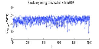
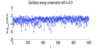
Figure 1: AAVF 1: the logarithm of the oscillatory energy errors against $t$.

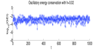
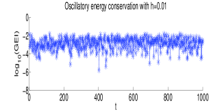
Figure 2: AAVF 2: the logarithm of the oscillatory energy errors against $t$.

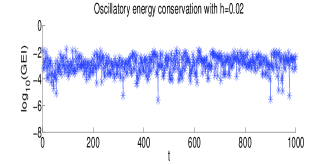
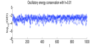
Figure 3: AAVF 3: the logarithm of the oscillatory energy errors against $t$.

3 Modulated Fourier expansion

In this section, we derive a modulated Fourier expansion of the AAVF method. The following assumptions are needed in our analysis.

Assumption 3.1

• The initial values of (1) are assumed to satisfy

  $$\frac{1}{2}\left\|p(0)\right\|^{2}+\frac{1}{2}\left\|\Omega q(0)\right\|^{2}\leq E$$ (7)

  with a constant $E$ independent of $\omega$.

• The numerical solution of the AAVF method is assumed to stay in a compact set.

• The stepsize is required to have a lower bound such that $h\omega\geq c_{0}>0.$

• We assume that the numerical non-resonance condition is true

  $$\left|\sin\big{(}\frac{1}{2}kh\omega\big{)}\right|\geq c\sqrt{h}\ \ \mathrm{for}\ \ k=1,2,\ldots,N\ \ \mathrm{with}\ \ N\geq 2.$$ (8)

These assumptions have been considered many times in the long-term analysis of other methods without EP property and we refer to [8, 14, 16] for example.

In this paper, we define five operators by

$$L_{1}(hD): =\mathrm{e}^{hD}-2\cos(h\Omega)+\mathrm{e}^{-hD},$$ (9)

$$L_{2}(hD): =\mathrm{e}^{\frac{1}{2}hD}+\mathrm{e}^{-\frac{1}{2}hD},$$

$$L_{3}(hD): =(\mathrm{e}^{hD}-1)(\mathrm{e}^{hD}+1)^{-1},$$

$$L_{4}(hD,\tau,k): =(1-\tau)\mathrm{e}^{-\mathrm{i}\frac{h}{2}k\omega}\mathrm{e}^{-\frac{h}{2}D}+\tau\mathrm{e}^{\mathrm{i}\frac{h}{2}k\omega}\mathrm{e}^{\frac{h}{2}D},$$

$$L(hD): =(L_{2}^{-1}L_{1})(hD),$$

where $D$ is the differential operator. The following properties of these operators will be used in our analysis.

Proposition 3.2

The Taylor expansions of $L(hD)$ are given by

$$L(hD)=\left(\begin{array}[]{cc}0&0\\ 0&1-\cos(h\omega)\\ \end{array}\right)-\frac{1}{8}\left(\begin{array}[]{cc}4&0\\ 0&3+\cos(h\omega)\\ \end{array}\right)(\textmd{i}hD)^{2}+\cdots,$$

$$L(hD+\mathrm{i}h\omega)=\left(\begin{array}[]{cc}-4\csc(h\omega)\sin^{3}(\frac{h\omega}{2})&0\\ 0&0\\ \end{array}\right)$$

$$+\left(\begin{array}[]{cc}\frac{3+\cos(h\omega)}{2}\sec(\frac{h\omega}{2})\tan(\frac{h\omega}{2})&0\\ 0&2\sin(\frac{h\omega}{2})\\ \end{array}\right)(\textmd{i}hD)+\cdots,$$

$$L(hD+\mathrm{i}kh\omega)=\left(\begin{array}[]{cc}-4\csc(kh\omega)\sin^{3}(\frac{kh\omega}{2})&0\\ 0&(\cos(kh\omega)-\cos(h\omega))\sec(\frac{kh\omega}{2})\\ \end{array}\right)$$

$$+\left(\begin{array}[]{cc}\frac{3+\cos(kh\omega)}{2}\sec(\frac{kh\omega}{2})\tan(\frac{kh\omega}{2})&0\\ 0&\frac{2+\cos(kh\omega)+\cos(h\omega)}{2}\sec(\frac{kh\omega}{2})\tan(\frac{kh\omega}{2})\\ \end{array}\right)(\textmd{i}hD)+\cdots$$

for $\left|k\right|>1$. The operator $L_{3}(hD)$ can be expressed in its Taylor expansions as follows:

$$L_{3}(hD)=\frac{1}{2}(hD)-\frac{1}{24}(hD)^{3}+\cdots,$$

$$L_{3}(hD+\mathrm{i}kh\omega)=\tan(\frac{kh\omega}{2})\textmd{i}+\frac{1}{1+\cos(kh\omega)}(hD)+\cdots$$

for $\left|k\right|>0$. Moreover, for the operator $L_{4}(hD,\tau,k)$ with $\left|k\right|>0$, the following result holds

$$L_{4}(hD,\frac{1}{2},k)=\cos(\frac{kh\omega}{2})+\frac{1}{2}\sin(\frac{kh\omega}{2})(\textmd{i}hD)+\cdots.$$

Theorem 3.3

Suppose that the conditions given in Assumption 3.1 are true. The numerical solution of the AAVF method (5) admits the following modulated Fourier expansion for $0\leq t=nh\leq T$:

$$q_{n}=\sum\limits_{|k|<N}\mathrm{e}^{\mathrm{i}k\omega t}\zeta_{h}^{k}(t)+R_{h,N}(t),\ \ p_{n}=\sum\limits_{|k|<N}\mathrm{e}^{\mathrm{i}k\omega t}\eta_{h}^{k}(t)+S_{h,N}(t),$$ (10)

where $N$ is a fixed integer determined by (8) and the remainder terms are bounded by

$$R_{h,N}(t)=\mathcal{O}(h^{N}),\ \ \ \ S_{h,N}(t)=\mathcal{O}(h^{N-1}).\\$$ (11)

The coefficient functions $\zeta_{h}^{k},\eta_{h}^{k}$ as well as all their derivatives are bounded by

$$\zeta^{0}_{h,1}=\mathcal{O}(1),\qquad\quad\eta^{0}_{h,1}=\mathcal{O}(1),\ \ \qquad\zeta^{0}_{h,2}=\mathcal{O}(h^{2}),\quad\ \ \ \ \ \eta^{0}_{h,2}=\mathcal{O}(h^{\frac{3}{2}}),$$ (12)

$$\zeta^{1}_{h,1}=\mathcal{O}(h^{2}),\ \ \ \ \ \ \ \eta^{1}_{h,1}=\mathcal{O}(h),\quad\ \ \ \ \ \zeta^{1}_{h,2}=\mathcal{O}(h),\quad\ \ \ \ \ \ \eta^{1}_{h,2}=\textmd{i}\omega\zeta^{1}_{h,2}+\mathcal{O}(h),$$

$$\zeta^{k}_{h,1}=\mathcal{O}(h^{k+1}),\quad\ \eta^{k}_{h,1}=\mathcal{O}(h^{k}),\quad\ \ \ \ \zeta^{k}_{h,2}=\mathcal{O}(h^{k+1}),\quad\ \ \eta^{k}_{h,2}=\mathcal{O}(h^{k})$$

for $k=2,\ldots,N-1$. Moreover, we have $\zeta^{-k}=\overline{\zeta^{k}}$ and $\eta^{-k}=\overline{\eta^{k}}$. The constants symbolised by the notation depend on the constants from Assumption 3.1 and the final time $T$, but are independent of $h$ and $\omega$.

Proof  In this proof, we will construct the functions

$$q_{h}(t)=\sum\limits_{|k|<N}\mathrm{e}^{\mathrm{i}k\omega t}\zeta_{h}^{k}(t),\quad\ p_{h}(t)=\sum\limits_{|k|<N}\mathrm{e}^{\mathrm{i}k\omega t}\eta_{h}^{k}(t)$$ (13)

with smooth coefficient functions $\zeta_{h}^{k}$ and $\eta_{h}^{k}$, such that there is only a small defect when (13) is inserted into the numerical scheme (5).

I. Construction of the coefficients functions.

It follows from the symmetry of the AAVF method that

$$q_{n+1}-2\cos(h\Omega)q_{n}+q_{n-1}$$ (14)

$$= h^{2}\phi_{2}(V)\big{[}\int_{0}^{1}f((1-\tau)q_{n}+\tau q_{n+1})d\tau+\int_{0}^{1}f((1-\tau)q_{n}+\tau q_{n-1})d\tau\big{]}$$

$$= h^{2}\phi_{2}(V)\big{[}\int_{0}^{1}f((1-\tau)q_{n}+\tau q_{n+1})d\tau+\int_{0}^{1}f((1-\tau)q_{n-1}+\tau q_{n})d\tau\big{]},$$

where we have used the following property

$$\int_{0}^{1}f((1-\tau)q_{n}+\tau q_{n-1})d\tau=\displaystyle\int_{0}^{1}f((1-\tau)q_{n-1}+\tau q_{n})d\tau.$$

For the term $(1-\tau)q_{n}+\tau q_{n+1}$, we look for a function of the form

$$\tilde{q}_{h}(t+\frac{h}{2},\tau)=\sum\limits_{|k|<N}\mathrm{e}^{\mathrm{i}k\omega(t+\frac{h}{2})}\xi_{h}^{k}(t+\frac{h}{2},\tau)$$

as its modulated Fourier expansion. Then one has

$$\tilde{q}_{h}(t+\frac{h}{2},\tau) =(1-\tau)\sum\limits_{|k|<N}\mathrm{e}^{\mathrm{i}k\omega t}\zeta_{h}^{k}(t)+\tau\sum\limits_{|k|<N}\mathrm{e}^{\mathrm{i}k\omega(t+h)}\zeta_{h}^{k}(t+h)$$

$$=\sum\limits_{|k|<N}\mathrm{e}^{\mathrm{i}k\omega(t+\frac{h}{2})}\Big{(}(1-\tau)\mathrm{e}^{-\mathrm{i}k\omega\frac{h}{2}}\mathrm{e}^{-\frac{h}{2}D}+\tau\mathrm{e}^{\mathrm{i}k\omega\frac{h}{2}}\mathrm{e}^{\frac{h}{2}D}\Big{)}\zeta_{h}^{k}(t+\frac{h}{2}),$$

which yields

$$\xi_{h}^{k}(t+\frac{h}{2},\tau)= \Big{(}(1-\tau)\mathrm{e}^{-\mathrm{i}k\omega\frac{h}{2}}\mathrm{e}^{-\frac{h}{2}D}+\tau\mathrm{e}^{\mathrm{i}k\omega\frac{h}{2}}\mathrm{e}^{\frac{h}{2}D}\Big{)}\zeta_{h}^{k}(t+\frac{h}{2})$$ (15)

$$= L_{4}(hD,\tau,k)\zeta_{h}^{k}(t+\frac{h}{2}).$$

Similarly, for $(1-\tau)q_{n-1}+\tau q_{n}$, we have the following modulated Fourier expansion

$$\tilde{q}_{h}(t-\frac{h}{2},\tau)=\sum\limits_{|k|<N}\mathrm{e}^{\mathrm{i}k\omega(t-\frac{h}{2})}\xi_{h}^{k}(t-\frac{h}{2},\tau)$$

with

$$\xi_{h}^{k}(t-\frac{h}{2},\tau)=\Big{(}(1-\tau)\mathrm{e}^{-\mathrm{i}k\omega\frac{h}{2}}\mathrm{e}^{-\frac{h}{2}D}+\tau\mathrm{e}^{\mathrm{i}k\omega\frac{h}{2}}\mathrm{e}^{\frac{h}{2}D}\Big{)}\zeta_{h}^{k}(t-\frac{h}{2})=L_{4}(hD,\tau,k)\zeta_{h}^{k}(t-\frac{h}{2}).$$ (16)

Inserting these modulated Fourier expansions into (14) implies

$$q_{h}(t+h)-2\cos(h\Omega)q_{h}(t)+q_{h}(t-h)$$

$$= h^{2}\phi_{2}(V)\big{[}\int_{0}^{1}f(\tilde{q}_{h}(t+\frac{h}{2},\tau))d\tau+\int_{0}^{1}f(\tilde{q}_{h}(t-\frac{h}{2},\tau))d\tau\big{]}.$$

According to the definitions given in (9), this result can be rewritten as

$$L_{1}(hD)q_{h}(t)=h^{2}\phi_{2}(V)L_{2}(hD)\int_{0}^{1}f(\tilde{q}_{h}(t,\tau))d\tau,$$

which means

$$L(hD)q_{h}(t)=h^{2}\phi_{2}(V)\int_{0}^{1}f(\tilde{q}_{h}(t,\tau))d\tau.$$

By expanding the nonlinear function $f$ at $\xi_{h}^{0}(t)$ into its Taylor series, and comparing the coefficients of $\mathrm{e}^{\mathrm{i}k\omega t}$, one arrives at

$$L(hD)\zeta_{h}^{0}(t)=h^{2}\phi_{2}(V)\int_{0}^{1}\Big{(}f(\xi_{h}^{0}(t,\tau))+\sum\limits_{s(\alpha)=0}\frac{1}{m!}f^{(m)}(\xi_{h}^{0}(t,\tau))(\xi_{h}(t,\tau))^{\alpha}\Big{)}d\tau,$$

$$L(hD+\mathrm{i}kh\omega)\zeta_{h}^{k}(t)=h^{2}\phi_{2}(V)\int_{0}^{1}\sum\limits_{s(\alpha)=k}\frac{1}{m!}f^{(m)}(\xi_{h}^{0}(t,\tau))(\xi_{h}(t,\tau))^{\alpha}d\tau,\qquad k\neq 0,$$

where the sum ranges over $m\geq 0$, $\alpha=(\alpha_{1},\ldots,\alpha_{m})$ with integer $\alpha_{i}$ satisfying $0<|\alpha_{i}|<N$, $s(\alpha)=\sum\limits_{j=1}^{m}\alpha_{j},$ and $(\xi_{h}(t,\tau))^{\alpha}$ is an abbreviation for $(\xi_{h}^{\alpha_{1}}(t,\tau),\ldots,\xi_{h}^{\alpha_{m}}(t,\tau))$. This formula as well as (15) and (16) gives the modulation system for the coefficients $\zeta_{h}^{k}(t)$ of the modulated Fourier expansion $q_{n}$. Considering the dominate terms in the relations motivates the following ansatz:

$$\begin{array}[c]{rll}&\ddot{\zeta}^{0}_{h,1}(t)=G^{0}_{\pm 10}(\cdot)+\cdots,&\zeta^{0}_{h,2}(t)=\frac{1}{\omega^{2}}\big{(}G^{0}_{\pm 20}(\cdot)+\cdots\big{)},\\ &\zeta^{1}_{h,1}(t)=\frac{-h^{2}\cos(\frac{h\omega}{2})}{4\sin^{2}(\frac{h\omega}{2})}\big{(}G^{1}_{\pm 10}(\cdot)+\cdots\big{)},&\dot{\zeta}^{1}_{h,2}(t)=\frac{-\textmd{i}}{2\omega}\mathrm{sinc}(\frac{h\omega}{2})\big{(}G^{1}_{\pm 20}(\cdot)+\cdots\big{)},\\ &\zeta^{k}_{h,1}(t)=\frac{-h^{2}\cos(\frac{kh\omega}{2})}{4\sin^{2}(\frac{kh\omega}{2})}\big{(}G^{k}_{\pm 10}(\cdot)+\cdots\big{)},&\zeta^{k}_{h,2}(t)=\frac{h^{2}\phi_{2}(h\omega)\cos(\frac{kh\omega}{2})}{-2\sin(\frac{k+1}{2}h\omega)\sin(\frac{k-1}{2}h\omega)}\big{(}G^{k}_{\pm 20}(\cdot)+\cdots\big{)},\end{array}$$ (17)

where the dots stand for power series in $\sqrt{h}$. Following [14, 15], we truncate the ansatz after the $\mathcal{O}(h^{N+1})$ terms.

Using the scheme of the AAVF method (5) again, it is obtained that

$$q_{n+1} =\phi_{0}(V)q_{n}+h\phi_{1}(V)p_{n}+h\phi_{2}(V)\phi_{1}^{-1}(V)(p_{n+1}+h\Omega^{2}\phi_{1}(V)q_{n}-\phi_{0}(V)p_{n}),$$

which can be simplified as

$$q_{n+1}-\big{(}\phi_{0}(V)+V\phi_{2}(V)\big{)}q_{n}=h\phi_{2}(V)\phi_{1}^{-1}(V)p_{n+1}+h\big{(}\phi_{1}(V)-\phi_{0}(V)\phi_{1}^{-1}(V)\phi_{2}(V)\big{)}p_{n}.$$

According to the definition of $\phi$-functions given by (6), it can be verified straightforwardly that

$$\phi_{0}(V)+V\phi_{2}(V)=I,$$

$$\phi_{2}(V)\phi_{1}^{-1}(V)=\phi_{1}(V)-\phi_{0}(V)\phi_{1}^{-1}(V)\phi_{2}(V)=\tan(\frac{1}{2}h\Omega)(h\Omega)^{-1}.$$

We then obtain

$$q_{n+1}-q_{n}=\Omega^{-1}\tan(\frac{1}{2}h\Omega)(p_{n+1}+p_{n}).$$ (18)

By the definition of $L_{3}$, this relation can be expressed as

$$L_{3}(hD)q_{h}(t)=\Omega^{-1}\tan(\frac{1}{2}h\Omega)p_{h}(t).$$

Therefore, we get the modulation system for the coefficients $\eta_{h}^{k}(t)$ of the modulated Fourier expansion $p_{n}$ as

$$\eta_{h}^{0}(t)=\Omega\tan^{-1}(\frac{1}{2}h\Omega)L_{3}(hD)\zeta_{h}^{0}(t),\ \ \eta_{h}^{k}(t)=\Omega\tan^{-1}(\frac{1}{2}h\Omega)L_{3}(hD+\mathrm{i}kh\omega)\zeta_{h}^{k}(t)$$ (19)

for $k\neq 0.$ In the light of the Taylor series of $L_{3}$, one has the following relationship between $\eta_{h}^{k}$ and $\zeta_{h}^{k}$:

$$\begin{array}[c]{rll}&\eta^{0}_{h,1}(t)=\dot{\zeta}^{0}_{h,1}(t)+\mathcal{O}(h^{2}),&\eta^{0}_{h,2}(t)=\frac{\cos(\frac{h\omega}{2})}{\mathrm{sinc}(\frac{h\omega}{2})}\dot{\zeta}^{0}_{h,2}(t)+\mathcal{O}(h),\\ &\eta^{1}_{h,1}(t)=\textmd{i}\omega\frac{\mathrm{sinc}(\frac{h\omega}{2})}{\cos(\frac{h\omega}{2})}\zeta^{1}_{h,1}(t)+\mathcal{O}(h),&\eta^{1}_{h,2}=\textmd{i}\omega\zeta^{1}_{h,2}+\mathcal{O}(h),\\ &\eta^{k}_{h,1}(t)=\textmd{i}k\omega\frac{\mathrm{sinc}(\frac{kh\omega}{2})}{\cos(\frac{kh\omega}{2})}\zeta^{k}_{h,1}(t)+\mathcal{O}(h),&\eta^{k}_{h,2}(t)=\textmd{i}\omega\frac{\tan(\frac{kh\omega}{2})}{\tan(\frac{h\omega}{2})}\zeta^{k}_{h,2}+\mathcal{O}(h),\end{array}$$ (20)

where $\left|k\right|>1.$ This presents the modulation equation of $\eta_{h}^{k}$.

II. Initial values. By the conditions that (10) is satisfied without the remainder term for $t=0$ and $t=h$, the initial values for the differential equations of $\zeta^{0}_{h,1}$ and $\zeta^{1}_{h,2}$ can be determined as follows.

Considering the conditions $p_{h}(0)=p_{0}$ and $q_{h}(0)=q_{0}$, we get

$$p_{0,1}=\eta_{h,1}^{0}(0)+\mathcal{O}(h)=\dot{\zeta}^{0}_{h,1}(0)+\mathcal{O}(h),$$

$$q_{0,1}=\zeta_{h,1}^{0}(0)+\mathcal{O}(h),\ \ q_{0,2}=2\mathrm{Re}(\zeta^{1}_{h,2}(0))+\mathcal{O}(h^{2}).$$

This gives the initial values $\zeta_{h,1}^{0}(0),\dot{\zeta}^{0}_{h,1}(0)$ and $\mathrm{Re}(\zeta^{1}_{h,2}(0))$. Moreover, it follows from (7) that $q_{0,2}=\mathcal{O}(\omega^{-1}),$ which implies that $\mathrm{Re}(\zeta^{1}_{h,2}(0))=\mathcal{O}(h)$. In what follows, we derive the value of $\mathrm{Im}(\zeta^{1}_{h,2}(0))$.

From $q_{h,1}(h)=q_{1,1},\ q_{h,2}(h)=q_{1,2}$ and the first formula of AAVF method, it follows that

$$q_{1,2}-\cos(h\omega)q_{0,2}=h\mathrm{sinc}(h\omega)p_{0,2}+\mathcal{O}(h^{2}).$$

We compute

$$q_{1,2}-\cos(h\omega)q_{0,2}=q_{h,2}(h)-\cos(h\omega)q_{h,2}(0)$$

$$= \sum\limits_{|k|<N}\mathrm{e}^{\mathrm{i}k\omega h}\zeta_{h,2}^{k}(h)-\cos(h\omega)\sum\limits_{|k|<N}\zeta_{h,2}^{k}(0)$$

$$= \zeta_{h,2}^{0}(h)+\mathrm{e}^{\mathrm{i}\omega h}\zeta_{h,2}^{1}(h)+\mathrm{e}^{-\mathrm{i}\omega h}\zeta_{h,2}^{-1}(h)-\cos(h\omega)\Big{(}\zeta_{h,2}^{0}(0)+\zeta_{h,2}^{1}(0)+\zeta_{h,2}^{-1}(0)\Big{)}+\mathcal{O}(h^{2}).$$

Expanding the functions $\zeta_{h,2}^{0}(h),\ \zeta_{h,2}^{1}(h),\ \zeta_{h,2}^{-1}(h)$ at $h=0$ yields

$$q_{1,2}-\cos(h\omega)q_{0,2}= (1-\cos(h\omega))\zeta_{h,2}^{0}(0)+\mathrm{i}\sin(h\omega)(\zeta_{h,2}^{1}(0)-\zeta_{h,2}^{-1}(0))+\mathcal{O}(h^{2}).$$

It is clear from $1-\cos(h\omega)=\frac{1}{2}h^{2}\omega^{2}\mathrm{sinc}^{2}(h\omega/2)$ that

$$(1-\cos(h\omega))\zeta_{h,2}^{0}(0)=\frac{1}{2}h^{2}\omega^{2}\mathrm{sinc}^{2}(h\omega/2)\zeta_{h,2}^{0}(0)=2\sin^{2}(h\omega/2)\zeta_{h,2}^{0}(0)=\mathcal{O}(h^{2}).$$

Thus it is confirmed that

$$\mathrm{i}\sin(h\omega)(\zeta_{h,2}^{1}(0)-\zeta_{h,2}^{-1}(0))= h\mathrm{sinc}(h\omega)p_{0,2}+\mathcal{O}(h^{2}),$$

which yields $2\mathrm{Im}(\zeta_{h,2}^{1}(0))=\omega^{-1}p_{0,2}+\mathcal{O}(h)=\mathcal{O}(h).$

III. Bounds of the coefficients functions. Based on Assumption 3.1, the ansatz given by (17) and (20), and the initial values presented in the above part, the bounds shown in (12) are easily derived.

IV. Remainder. For $t=nh$, let

$$\delta_{q}(t+h)= q_{h}(t+h)-\phi_{0}(V)q_{h}(t)-h\phi_{1}(V)p_{h}(t)$$

$$-h^{2}\phi_{2}(V)\int_{0}^{1}f((1-\tau)q_{h}(t)+\tau q_{h}(t+h))d\tau,$$

$$\delta_{p}(t+h)= p_{h}(t+h)+h\Omega^{2}\phi_{1}(V)q_{h}(t)-\phi_{0}(V)p_{h}(t)$$

$$-h\phi_{1}(V)\int_{0}^{1}f((1-\tau)q_{h}(t)+\tau q_{h}(t+h))d\tau.$$

It is clear from the two-step formulation that $\delta_{q}(t+h)+\delta_{q}(t-h)=\mathcal{O}(h^{N+2})$. According to the choice for the initial values, we obtain $\delta_{q}(0)=\mathcal{O}(h^{N+2}).$ Thus it is derived that $\delta_{q}(t)=\mathcal{O}(h^{N+2})+\mathcal{O}(th^{N+1}).$ Then according to (18), one gets $\delta_{p}=\mathcal{O}(h^{N}).$ By letting $R_{n}=q_{n}-q_{h}(t)$ and $S_{n}=p_{n}-p_{h}(t),$ we obtain the following error recursion

$$\left(\begin{array}[]{c}\Omega R_{n+1}\\ S_{n+1}\\ \end{array}\right)=\left(\begin{array}[]{cc}\cos(h\Omega)&\sin(h\Omega)\\ -\sin(h\Omega)&\cos(h\Omega)\\ \end{array}\right)\left(\begin{array}[]{c}\Omega R^{n}\\ S^{n}\\ \end{array}\right)$$

$$+ h\left(\begin{array}[]{c}h\Omega\phi_{2}(V)\displaystyle\int_{0}^{1}\big{(}f((1-\tau)q_{n}+\tau q_{n+1})-f((1-\tau)q_{h}(t)+\tau q_{h}(t+h))\big{)}d\tau\\ \phi_{1}(V)\displaystyle\int_{0}^{1}\big{(}f((1-\tau)q_{n}+\tau q_{n+1})-f((1-\tau)q_{h}(t)+\tau q_{h}(t+h))\big{)}d\tau\\ \end{array}\right)$$

$$+ \left(\begin{array}[]{c}\Omega\delta_{q}\\ \delta_{p}\\ \end{array}\right).$$

By using the Lipschitz continuous of the nonlinearity, one obtains

$$\left\|f((1-\tau)q_{n}+\tau q_{n+1})-f((1-\tau)q_{h}(t)+\tau q_{h}(t+h))\right\|\leq\left\|R_{n}\right\|+\left\|R_{n+1}\right\|.$$

Then the remainder (11) can be derived by solving the error recursion and the application of a discrete Gronwall inequality.

The proof of this theorem is complete.

4 Long-time oscillatory energy conservation

This section is devoted to showing the long-time oscillatory energy conservation of the AAVF method.

Denote $\zeta=\big{(}\zeta^{-N+1}_{h},\cdots,\zeta^{-1}_{h},\zeta^{0}_{h},\zeta^{1}_{h},\cdots,\zeta^{N-1}_{h}\big{)}.$ The modulation functions of the AAVF method have the following almost invariant.

Theorem 4.1

Suppose that the conditions of Theorem 3.3 hold. For the coefficient functions of the modulated Fourier expansion, there exists a function $\widehat{\mathcal{I}}[\zeta]$ such that

$$\widehat{\mathcal{I}}[\zeta](t)=\widehat{\mathcal{I}}[\zeta](0)+\mathcal{O}(th^{N}),$$

where $0\leq t\leq T.$ Moreover, this almost invariant can be expressed as

$$\widehat{\mathcal{I}}[\zeta]=2\omega^{2}\frac{\cos(\frac{1}{2}h\omega)}{\mathrm{sinc}(\frac{1}{2}h\omega)}\big{(}\zeta_{h,2}^{-1}\big{)}^{\intercal}\zeta_{h,2}^{1}+\mathcal{O}(h^{2}).$$

Proof  With the proof of Theorem 3.3 proposed in the previous section, one obtains

$$L(hD)q_{h}(t)=h^{2}\phi_{2}(V)\int_{0}^{1}f(\tilde{q}_{h}(t,\tau))d\tau+\mathcal{O}(h^{N+2}),$$

where we use the following denotations:

$$q_{h}(t)=\sum\limits_{|k|<N}q^{k}_{h}(t),\ \ \tilde{q}_{h}(t,\tau)=\sum\limits_{|k|<N}\tilde{q}^{k}_{h}(t,\tau).$$

Here $q^{k}_{h}$ and $\tilde{q}^{k}_{h}$ are defined as $q^{k}_{h}(t)=\mathrm{e}^{\mathrm{i}k\omega t}\zeta_{h}^{k}(t)$ and $\tilde{q}^{k}_{h}(t,\tau)=\mathrm{e}^{\mathrm{i}k\omega t}\xi_{h}^{k}(t,\tau),$ respectively. By considering the definitions of $\tilde{q}_{h},\ q_{h}$ and comparing the coefficients of $\mathrm{e}^{\mathrm{i}k\omega t}$, we obtain the equations in terms of $q_{h}^{k}:$

$$L(hD)q^{k}_{h}(t)=-h^{2}\phi_{2}(V)\displaystyle\nabla_{-k}\mathcal{U}(\tilde{q}(t,\tau))+\mathcal{O}(h^{N+2}),$$

where $\mathcal{U}(\tilde{q}(t,\tau))$ is defined as

$$\mathcal{U}(\tilde{q}(t,\tau))=\int_{0}^{1}U(\tilde{q}^{0}_{h}(t,\tau))d\tau+\sum\limits_{s(\alpha)=0}\frac{1}{m!}\int_{0}^{1}U^{(m)}(\tilde{q}^{0}_{h}(t,\tau))(\tilde{q}_{h}(t,\tau))^{\alpha}d\tau,$$ (21)

and $\tilde{q}(t,\tau)$ is given by

$$\tilde{q}(t,\tau)=\big{(}\tilde{q}^{-N+1}_{h}(t,\tau),\ldots,\tilde{q}^{0}_{h}(t,\tau),\ldots,\tilde{q}^{N-1}_{h}(t,\tau)\big{)}.$$

Define a vector function $\tilde{q}(\lambda,t,\tau)$ of $\lambda$ as below

$$\tilde{q}(\lambda,t,\tau)=\big{(}\mathrm{e}^{\mathrm{i}(-N+1)\lambda\omega}\tilde{q}^{-N+1}_{h}(t,\tau),\cdots,\tilde{q}^{0}_{h}(t,\tau),\cdots,\mathrm{e}^{\mathrm{i}(N-1)\lambda\omega}\tilde{q}^{N-1}_{h}(t,\tau)\big{)}.$$

It can be observed from the definition (21) that $\mathcal{U}(\tilde{q}(\lambda,t,\tau))$ is independent of $\lambda$ and $\tau$. Thus, considering its derivative with respect to $\lambda$ implies

$$0= \frac{\partial}{\partial\lambda}\mathcal{U}(\tilde{q}(\lambda,t,\tau))=\Big{(}\frac{\partial}{\partial\tilde{q}}\mathcal{U}(\tilde{q}(\lambda,t,\tau))\Big{)}^{\intercal}\frac{\partial}{\partial\lambda}\tilde{q}(\lambda,t,\tau)$$

$$= \sum\limits_{|k|<N}\mathrm{i}k\omega\mathrm{e}^{\mathrm{i}k\lambda\omega}(\tilde{q}^{k}_{h}(\lambda,t,\tau))^{\intercal}\nabla_{k}\mathcal{U}(\tilde{q}(\lambda,t,\tau)).$$

The choice of $\lambda=0$ and $\tau=\frac{1}{2}$ yields $\sum\limits_{|k|<N}\mathrm{i}k\omega(\tilde{q}^{k}_{h}(t,\frac{1}{2}))^{\intercal}\nabla_{k}\mathcal{U}(\tilde{q}(t,\frac{1}{2}))=0.$ Therefore, one gets

$$0= \sum\limits_{|k|<N}\mathrm{i}k\omega(\tilde{q}^{-k}_{h}(t,\frac{1}{2}))^{\intercal}\nabla_{-k}\mathcal{U}(\tilde{q}(t,\frac{1}{2}))$$ (22)

$$= \sum\limits_{|k|<N}\mathrm{i}k\omega(\tilde{q}^{-k}_{h}(t,\frac{1}{2}))^{\intercal}\frac{1}{-h^{2}}\phi^{-1}_{2}(V)L(hD)q^{k}_{h}(t)+\mathcal{O}(h^{N}).$$

Inserting the expressions of $q^{k}_{h}$ and $\tilde{q}^{k}_{h}$ into (22) gives

$$\mathcal{O}(h^{N}) =\sum\limits_{|k|<N}\mathrm{i}k\omega(\xi_{h}^{-k}(t,\frac{1}{2}))^{\intercal}\frac{1}{-h^{2}}\phi^{-1}_{2}(V)L(hD+\mathrm{i}k\omega h)\zeta^{k}_{h}(t)$$ (23)

$$=\sum\limits_{|k|<N}\mathrm{i}k\omega(L_{4}(hD,\frac{1}{2},-k)\zeta_{h}^{-k}(t))^{\intercal}\frac{1}{-h^{2}}\phi^{-1}_{2}(V)L(hD+\mathrm{i}k\omega h)\zeta^{k}_{h}(t).$$

By Proposition 3.2, we get

$$L_{4}(hD,\frac{1}{2},-k)\zeta_{h}^{-k}(t)=(\cdot)\bar{\zeta}^{k}_{h}+\textmd{i}h(\cdot)\dot{\bar{\zeta}}^{k}_{h}+h^{2}(\cdot)\ddot{\bar{\zeta}}^{k}_{h}+\cdots,$$

$$L(hD+\mathrm{i}k\omega h)\zeta^{k}_{h}=(\cdot)\zeta^{k}_{h}+\textmd{i}h(\cdot)\dot{\zeta}^{k}_{h}+h^{2}(\cdot)\ddot{\zeta}^{k}_{h}+\cdots.$$

Looking closer to the right-hand side of (23), using the above expressions of $L_{4}$ and $L$, and considering the formulae on p. 508 of [16], it can be verified that the right-hand side of (23) is a total derivative. Therefore, there exists a function $\widehat{\mathcal{I}}$ such that $\frac{d}{dt}\widehat{\mathcal{I}}[\zeta](t)=\mathcal{O}(h^{N})$. An integration of it immediately implies the first statement of the theorem.

By the previous analysis and the bounds of Theorem 3.3, the construction of $\widehat{\mathcal{I}}$ is obtained as follows:

$$\widehat{\mathcal{I}}[\zeta]= 2\frac{2h\omega\sin(\frac{1}{2}h\omega)\cos(\frac{1}{2}h\omega)}{h^{2}\phi_{2}(h\omega)}\frac{1}{2}\big{(}\zeta_{h,2}^{-1}\big{)}^{\intercal}\zeta_{h,2}^{1}+\mathcal{O}(h^{2})$$

$$= 2\omega^{2}\frac{\cos(\frac{1}{2}h\omega)}{\mathrm{sinc}(\frac{1}{2}h\omega)}\big{(}\zeta_{h,2}^{-1}\big{)}^{\intercal}\zeta_{h,2}^{1}+\mathcal{O}(h^{2}).$$

We complete the proof of this theorem.

We are now in a position to present the main result of this paper.

Theorem 4.2

Define $\mathcal{I}[\zeta]=\widehat{\mathcal{I}}[\zeta]/\sigma(h\omega),$ where $\sigma(h\omega)$ is given by $\sigma(h\omega)=\frac{\cos(\frac{1}{2}h\omega)}{\mathrm{sinc}(\frac{1}{2}h\omega)}.$ Under the conditions of Theorem 3.3 and that $\left|\cos(\frac{1}{2}h\omega)\right|\geq ch^{m}$ for some $m$, we have the following relation between $\mathcal{I}[\zeta]$ and $I(q_{n},p_{n})$:

$$\mathcal{I}[\zeta](nh)=I(q_{n},p_{n})+\mathcal{O}(h).$$

Moreover, it holds that

$$I(q_{n},p_{n})=I(q_{0},p_{0})+\mathcal{O}(h)$$

for $0\leq nh\leq h^{-N+1}.$ The constants symbolized by $\mathcal{O}$ are independent of $n,h,\omega$, but depend on $N,T$ and the constants in the assumptions.

Proof  According to the definition of $\mathcal{I}$ and under the conditions of this theorem, one obtains

$$\mathcal{I}[\zeta]=2\omega^{2}\big{(}\zeta_{h,2}^{-1}\big{)}^{\intercal}\zeta_{h,2}^{1}+\mathcal{O}(h^{2}).$$ (24)

On the other hand, it follows from (12) that $\eta_{h,2}^{\pm 1}(t)=\pm\mathrm{i}\omega\zeta_{h,2}^{\pm 1}(t)+\mathcal{O}(h).$ Thus using the bounds of Theorem 3.3, we have

$$\omega q_{n,2} =\omega\big{(}\mathrm{e}^{\mathrm{i}\omega t}\zeta_{h,2}^{1}(t)+\mathrm{e}^{-\mathrm{i}\omega t}\zeta_{h,2}^{-1}(t)\big{)}+\mathcal{O}(h),$$

$$p_{n,2} =\mathrm{i}\omega\big{(}\mathrm{e}^{\mathrm{i}\omega t}\zeta_{h,2}^{1}(t)-\mathrm{e}^{-\mathrm{i}\omega t}\zeta_{h,2}^{-1}(t)\big{)}+\mathcal{O}(h).$$

This implies

$$I(q_{n},p_{n}) =\frac{1}{2}p_{n,2}^{\intercal}p_{n,2}+\frac{1}{2}\omega^{2}q_{n,2}^{\intercal}q_{n,2}$$ (25)

$$=\frac{1}{2}\left\|\mathrm{i}\omega\big{(}\mathrm{e}^{\mathrm{i}\omega t}\zeta_{h,2}^{1}(t)-\mathrm{e}^{-\mathrm{i}\omega t}\zeta_{h,2}^{-1}(t)\big{)}\right\|^{2}+\frac{1}{2}\left\|\omega\big{(}\mathrm{e}^{\mathrm{i}\omega t}\zeta_{h,2}^{1}(t)+\mathrm{e}^{-\mathrm{i}\omega t}\zeta_{h,2}^{-1}(t)\big{)}\right\|^{2}$$

$$=2\omega^{2}\big{(}\zeta_{h,2}^{-1}\big{)}^{\intercal}\zeta_{h,2}^{1}+\mathcal{O}(h),$$

where we have used the fact that $\left\|v+\bar{v}\right\|^{2}+\left\|v-\bar{v}\right\|^{2}=4\left\|v\right\|^{2}$. A comparison between (24) and (25) gives the first stated relation of this theorem. Following the identical argument given in Section XIII of [16], the result of the long-time oscillatory energy preservation can be obtained by patching together many intervals of length $h$.

Remark 4.3

From the analysis stated above for oscillatory energy conservation, it follows that the result of Theorem 4.2 cannot be improved even high order quadratures are chosen for the AAVF method (5), which explains the numerical phenomenon shown in Section 2.

5 Generalization of multi-frequency case

In this section, we are devoted to extending the analysis to a muti-frequency highly oscillatory Hamiltonian system with the following Hamiltonian function

$$\begin{array}[c]{ll}H(q,p)&=\dfrac{1}{2}\textstyle\sum\limits_{j=0}^{l}\Big{(}\left\|p_{j}\right\|^{2}+\dfrac{\lambda_{j}^{2}}{\epsilon^{2}}\left\|q_{j}\right\|^{2}\Big{)}+U(q),\end{array}$$ (26)

where $q=(q_{0},q_{1},\ldots,q_{l}),\ p=(p_{0},p_{1},\ldots,p_{l})$ with $q_{j},\ p_{j}\in\mathbb{R}^{d_{j}}$, $\lambda_{0}=0$ and $\lambda_{j}\geq 1$ are distinct real numbers for $j\geq 1$, $\epsilon$ is a small positive parameter, and $U(q)$ is a smooth potential function. It is well known that this system has the oscillatory energy of the $j$th frequency as

$$I_{j}(q,p)=\dfrac{1}{2}\Big{(}\left\|p_{j}\right\|^{2}+\dfrac{\lambda_{j}^{2}}{\epsilon^{2}}\left\|q_{j}\right\|^{2}\Big{)},$$

and its total oscillatory energy is $I(q,p)=\sum\limits_{j=1}^{l}I_{j}(q,p).$

Muti-frequency highly oscillatory Hamiltonian system often arises in a wide range of applications, such as in physics and engineering, astronomy, molecular dynamics, and in problems of wave propagation in classical and quantum physics. There have been many efficient numerical methods for solving this system and we refer to [16, 17, 18, 32, 33, 37, 38, 40] as well as the references contained therein. This muti-frequency Hamiltonian system can also be rewritten as the highly oscillatory second-order system (4) with $\Omega=\textmd{diag}(\omega_{0}I_{d_{0}},\omega_{1}I_{d_{1}},\ldots,\omega_{l}I_{d_{l}})$, where $\omega_{j}=\lambda_{j}/\epsilon$. Thus the AAVF method (5) can be used to solve this system. In what follows, we briefly discuss the long-time oscillatory energies conservations of the AAVF method for this muti-frequency highly oscillatory Hamiltonian system. The technique used here is the muti-frequency modulated Fourier expansion of the AAVF method, which can be obtained by the generalization of Sections 3-4 of this paper and following the way used in [8]. For brevity, we just present the main results and omit the details of proof.

5.1 The main results for multi-frequency case

Let

$$\lambda=(\lambda_{1},\ldots,\lambda_{l}),\quad k=(k_{1},\ldots,k_{l}),\quad k\cdot\lambda=k_{1}\lambda_{1}+\cdots+k_{l}\lambda_{l},$$

and denote the resonance module by

$$\mathcal{M}=\{k\in\mathbb{Z}^{l}:\ k\cdot\lambda=0\}.$$ (27)

Following [8], we use the following notations

$$\omega=(\omega_{1},\ldots,\omega_{l}),\quad\langle j\rangle=(0,\ldots,1,\ldots,0),\quad|k|=|k_{1}|+\cdots+|k_{l}|.$$

For the resonance module (27), denote by $\mathcal{K}$ the set of representatives of the equivalence classes in $\mathbb{Z}^{l}\backslash\mathcal{M}$ which are chosen such that for each $k\in\mathcal{K}$ the sum $|k|$ is minimal in the equivalence class $[k]=k+\mathcal{M},$ and that with $k\in\mathcal{K}$, also $-k\in\mathcal{K}.$ For the positive integer $N$, we let

$$\mathcal{N}=\{k\in\mathcal{K}:\ |k|\leq N\},\ \ \ \ \ \mathcal{N}^{*}=\mathcal{N}\backslash\{(0,\ldots,0)\}.$$

The multi-frequency modulated Fourier expansion of the AAVF method is presented in the following theorem.

Theorem 5.1

The initial values are supposed to satisfy $H(q_{0},p_{0})\leq E$. Assume that $h/\epsilon\geq c_{0}>0$ and the following numerical non-resonance condition is true

$$|\sin(\frac{h}{2\epsilon}(k\cdot\lambda))|\geq c\sqrt{h}\ \ \mathrm{for}\ \ k\in\mathbb{Z}^{l}\backslash\mathcal{M}\ \ \mathrm{with}\ \ |k|\leq N$$

for some $N\geq 2$ and $c>0$. Then the AAVF method admits the following multi-frequency modulated Fourier expansion

$$q_{n}=\zeta(t)+\sum\limits_{k\in\mathcal{N}^{*}}\mathrm{e}^{\mathrm{i}(k\cdot\omega)t}\zeta^{k}(t)+\mathcal{O}(h^{N}),\ \ p_{n}=\eta(t)+\sum\limits_{k\in\mathcal{N}^{*}}\mathrm{e}^{\mathrm{i}(k\cdot\omega)t}\eta^{k}(t)+\mathcal{O}(h^{N-1}),$$

for $0\leq t=nh\leq T$. The coefficient functions as well as all their derivatives are bounded by

$$\begin{array}[c]{rll}&\zeta_{0}(t)=\mathcal{O}(1),&\eta_{0}(t)=\mathcal{O}(1),\\ &\zeta_{j}(t)=\mathcal{O}(h^{2}),&\eta_{j}(t))=\mathcal{O}(h),\\ &\zeta_{j}^{\pm\langle j\rangle}(t)=\mathcal{O}(h),&\eta_{j}^{\pm\langle j\rangle}(t)=\mathcal{O}(1),\\ &\zeta_{0}^{k}(t)=\mathcal{O}\big{(}h^{|k|+1}\big{)},&\eta_{0}^{k}(t)=\mathcal{O}\big{(}h^{|k|}\big{)},\ k\in\mathcal{N}^{*},\\ &\zeta_{j}^{k}(t)=\mathcal{O}\big{(}h^{|k|+1}\big{)},&\eta_{j}^{k}(t)=\mathcal{O}\big{(}h^{|k|}\big{)},\ \ k\neq\pm\langle j\rangle,\end{array}$$

for $j=1,\ldots,l$.

An almost-invariant is obtained for the functions of the multi-frequency modulated Fourier expansion.

Theorem 5.2

Under the conditions of Theorem 5.1, there exists a function $\widehat{\mathcal{I}}[\zeta]$ such that

$$\widehat{\mathcal{I}}_{\mu}[\zeta](t)=\widehat{\mathcal{I}}_{\mu}[\zeta](0)+\mathcal{O}(th^{N})+\mathcal{O}(t\epsilon^{M-1})$$

for all $\mu\in\mathbb{R}^{l}$ and $0\leq t\leq T.$ Here $M=\min\{|k|:0\neq k\in\mathcal{M}\}$. The almost-invariant satisfies

$$\widehat{\mathcal{I}}_{\mu}[\zeta](t)=\widehat{\mathcal{I}}_{\mu}[\zeta](0)+\mathcal{O}(th^{N})$$

for $\mu\perp\mathcal{M}_{N}:=\{k\in\mathcal{M}:\ |k|\leq N\}$ and $0\leq t\leq T.$ Moreover, $\widehat{\mathcal{I}}_{\mu}$ can be expressed in

$$\widehat{\mathcal{I}}_{\mu}[\zeta]= \sum\limits_{j=1}^{l}2\omega_{j}^{2}\frac{\mu_{j}}{\lambda_{j}}\frac{\cos(\frac{1}{2}h\omega_{j})}{\mathrm{sinc}(\frac{1}{2}h\omega_{j})}\big{(}\zeta_{j}^{-\langle j\rangle}\big{)}^{\intercal}\zeta_{j}^{\langle j\rangle}+\mathcal{O}(h).$$

Consider the following modified oscillatory energies

$$I_{\mu}^{*}(q,p)=\sum\limits_{j=1}^{l}\sigma(\xi_{j})\frac{\mu_{j}}{\lambda_{j}}I_{j}(q,p),$$

where $\sigma$ is defined as $\sigma(\xi_{j}):=\frac{\cos(\frac{1}{2}\xi_{j})}{\mathrm{sinc}(\frac{1}{2}\xi_{j})}.$ We then obtain the result about the long-time modified oscillatory energies conservations of the AAVF method for multi-frequency highly oscillatory systems.

Theorem 5.3

Under the conditions of Theorem 5.1, we have

$$\widehat{\mathcal{I}}_{\mu}[\vec{\zeta},\vec{\eta}](nh)=I_{\mu}^{*}(q_{n},p_{n})+\mathcal{O}(h).$$

Moreover, it holds that

$$I_{\mu}^{*}(q^{n},p^{n}) =I_{\mu}^{*}(q^{0},p^{0})+\mathcal{O}(h)$$

for $0\leq nh\leq h^{-N+1}$, $\mu\in\mathbb{R}^{l}$ and $\mu\perp\mathcal{M}_{N}$. The constants symbolised by $\mathcal{O}$ are independent of $n,h,\Omega$, but depend on $N,T$ and the constants in the assumptions.

5.2 Numerical experiments

In order to illustrate the numerical conservation of the modified oscillatory energies for the AAVF method, we consider a Hamiltonian (26) with $l=3$ and $\lambda=(1,\sqrt{2},2)$ (see [8]). It is shown in [8] that there is the $1:2$ resonance between $\lambda_{1}$ and $\lambda_{3}$: $\mathcal{M}=\{(-2k_{3},0,k_{3}):\ k_{3}\in\mathbb{Z}\}.$ For this problem, the dimension of $q_{1}=(q_{11},q_{12})$ is assumed to be 2 and all the other $q_{j}$ are assumed to be 1. We consider $\epsilon^{-1}=\omega=70$, the potential $U(q)=(0.001q_{0}+q_{11}+q_{22}+q_{2}+q_{3})^{4},$ and

$$q(0)=(1,0.3\epsilon,0.8\epsilon,-1.1\epsilon,0.7\epsilon),\ \ p(0)=(-0.75,0.6,0.7,-0.9,0.8)$$

as initial values. For $\lambda=(1,\sqrt{2},2),$ it is chosen that $\mu=(1,0,2)$ and $\mu=(0,\sqrt{2},0)$ for $I_{\mu}$ and the corresponding results are $I_{\mu}=I_{1}+I_{3}$ and $I_{\mu}=I_{2}.$ We integrate this problem on the interval $[0,10000]$ with $h=0.1,0,01$. The modified oscillatory energies conservations are shown in Figs. 4-6.

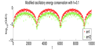
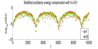
Figure 4: AAVF 1: the logarithm of the modified oscillatory energy errors against $t$.

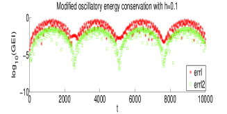
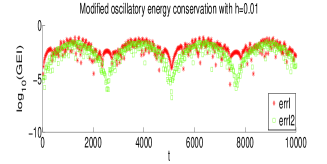
Figure 5: AAVF 2: the logarithm of the modified oscillatory energy errors against $t$.

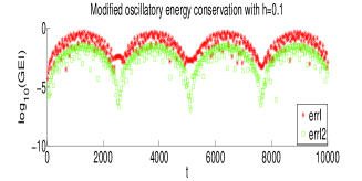
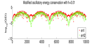
Figure 6: AAVF 3: the logarithm of the modified oscillatory energy errors against $t$.

6 Conclusions

In this paper, we presented a long-term analysis of the adapted average vector field (AAVF) method for highly oscillatory Hamiltonian systems. This AAVF method can exactly preserve the total energy of the underlying systems, but the main theme of this paper is to study its oscillatory energy and the corresponding numerical conservation. We analysed the long-term behaviour in the oscillatory energy conservation by developing modulated Fourier expansions for the method. A further extension of the analysis to multi-frequency case has also been discussed.

Last but not least, it is noted that some trigonometric energy-preserving methods have been well developed for solving wave equations and see [21, 22, 23, 36] for example. For Hamiltonian wave equations, the study of long-time conservation of momentum and actions along these EP methods is overarching importance, and this will be discussed in our another work.

References

• [1] P. Betsch, and P. Steinmann, Inherently energy conserving time finite elements for classical mechanics, J. Comput. Phys., 160 (2000), pp. 88-116.
• [2] L. Brugnano, F. Iavernaro, and D. Trigiante, Hamiltonan Boundary Value Methods (Energy Preserving Discrete Line Integral Methods), J. Numer. Anal. Ind. Appl. Math., 5 (2010), pp. 13-17.
• [3] L. Brugnano, F. Iavernaro, and D. Trigiante, Energy- and quadratic invariants-preserving integrators based upon Gauss-Collocation formulae, SIAM J. Numer. Anal., 50 (2012), pp. 2897-2916.
• [4] E. Celledoni, R. I. Mclachlan, B. Owren, and G. R. W. Quispel, Energy-preserving integrators and the structure of B-series, Found. Comput. Math., 10 (2010), pp. 673-693.
• [5] E. Celledoni, B. Owren, and Y. Sun, The minimal stage, energy preserving Runge–Kutta method for polynomial Hamiltonian systems is the averaged vector field method, Math. Comput., 83 (2014), pp. 1689-1700.
• [6] D. Cohen, L. Gauckler, E. Hairer, and C. Lubich, Long-term analysis of numerical integrators for oscillatory Hamiltonian systems under minimal non-resonance conditions, BIT, 55 (2015), pp. 705-732.
• [7] D. Cohen, and E. Hairer, Linear energy-preserving integrators for Poisson systems, BIT, 51 (2011), pp. 91-101.
• [8] D. Cohen, E. Hairer, and C. Lubich, Numerical energy conservation for multi-frequency oscillatory differential equations, BIT, 45 (2005), pp. 287-305.
• [9] L. Gauckler, Numerical long-time energy conservation for the nonlinear Schrödinger equation, IMA J. Numer. Anal., 37 (2017), pp. 2067-2090.
• [10] L. Gauckler, E. Hairer, and C. Lubich, Energy separation in oscillatory Hamiltonian systems without any non-resonance condition, Comm. Math. Phys., 321 (2013), pp. 803-815.
• [11] L. Gauckler, and C. Lubich, Splitting integrators for nonlinear Schrödinger equations over long times, Found. Comput. Math., 10 (2010), pp. 275-302.
• [12] E. Hairer, Energy-preserving variant of collocation methods, J. Numer. Anal. Ind. Appl. Math., 5 (2010), pp. 73-84.
• [13] E. Hairer, and C. Lubich, Energy conservation by Störmer-type numerical integrators, Numerical Analysis 1999 (D. F. Griffiths G. A. Watson, ed.), CRC Press LLC, (2000), pp. 169-190.
• [14] E. Hairer, and C. Lubich, Long-time energy conservation of numerical methods for oscillatory differential equations, SIAM J. Numer. Anal., 38 (2000), pp. 414-441.
• [15] E. Hairer, and C. Lubich, Long-term analysis of the Störmer-Verlet method for Hamiltonian systems with a solution-dependent high frequency, Numer. Math. ,134 (2016), pp. 119-138.
• [16] E. Hairer, C. Lubich, and G. Wanner, Geometric Numerical Integration: Structure-Preserving Algorithms for Ordinary Differential Equations, 2nd edn. Springer-Verlag, Berlin, Heidelberg, 2006.
• [17] M. Hochbruck, and A. Ostermann, Exponential integrators, Acta Numer., 19 (2010), pp. 209-286.
• [18] M. Hochbruck, and A. Ostermann, J. Schweitzer, Exponential rosenbrock-type methods, SIAM J. Numer. Anal., 47 (2009), pp. 786-803.
• [19] Y.W. Li, and X. Wu, Exponential integrators preserving first integrals or Lyapunov functions for conservative or dissipative systems, SIAM J. Sci. Comput., 38 (2016), pp. 1876-1895.
• [20] Y.W. Li, and X. Wu, Functionally fitted energy-preserving methods for solving oscillatory nonlinear Hamiltonian systems, SIAM J. Numer. Anal., 54 (2016), pp. 2036-2059.
• [21] C. Liu, and X. Wu, An energy-preserving and symmetric scheme for nonlinear Hamiltonian wave equations, J. Math. Anal. Appl., 440 (2016), pp. 167-182.
• [22] C. Liu, A. Iserles, and X. Wu, Symmetric and arbitrarily high-order Birkhoff–Hermite time integrators and their long-time behaviour for solving nonlinear Klein–Gordon equations, J. Comput. Phys., 356 (2018), pp. 1-30.
• [23] K. Liu, X. Wu, and W. Shi, A linearly-fitted conservative (dissipative) scheme for efficiently solving conservative (dissipative) nonlinear wave PDEs, J. Comput. Math., 35 (2017), pp. 780-800.
• [24] R. I. McLachlan, and G. R. W. Quispel, Discrete gradient methods have an energy conservation law, Disc. Contin. Dyn. Syst., 34 (2014), pp. 1099-1104.
• [25] R. I. McLachlan, G. R. W. Quispel, and N. Robidoux, Geometric integration using discrete gradient, Philos. Trans. R. Soc. Lond. A, 357 (1999), pp. 1021-1045.
• [26] R.I. McLachlan, and A. Stern, Modified trigonometric integrators, SIAM J. Numer. Anal., 52 (2014), pp. 1378-1397.
• [27] Y. Miyatake, An energy-preserving exponentially-fitted continuous stage Runge–Kutta method for Hamiltonian systems, BIT, 54 (2014), pp. 777-799.
• [28] Y. Miyatake, A derivation of energy-preserving exponentially-fitted integrators for Poisson systems, Comput. Phys. Comm., 187 (2015), pp. 156-161.
• [29] G. R. W. Quispel, and D. I. McLaren, A new class of energy-preserving numerical integration methods, J. Phys. A, 41 (045206) (2008), 7pp.
• [30] J.M. Sanz-Serna, Modulated Fourier expansions and heterogeneous multiscale methods, IMA J. Numer. Anal., 29 (2009), pp. 595-605.
• [31] A. Stern, and E. Grinspun, Implicit-explicit variational integration of highly oscillatory problems, Multi. Model. Simul., 7 (2009), pp. 1779-1794.
• [32] B. Wang, A. Iserles, and X. Wu, Arbitrary-order trigonometric Fourier collocation methods for multi-frequency oscillatory systems, Found. Comput. Math., 16 (2016), pp. 151-181.
• [33] B. Wang, F. Meng, and Y. Fang, Efficient implementation of RKN-type Fourier collocation methods for second-order differential equations, Appl. Numer. Math., 119 (2017), pp. 164-178.
• [34] B. Wang, and X. Wu, A new high precision energy preserving integrator for system of oscillatory second-order differential equations, Phys. Lett. A, 376 (2012), pp. 1185-1190.
• [35] B. Wang, and X. Wu, Functionally-fitted energy-preserving integrators forPoissonsystems, J. Comput. Phys., 364 (2018), pp. 137-152.
• [36] B. Wang, and X. Wu, The formulation and analysis of energy-preserving schemes for solving high-dimensional nonlinear Klein-Gordon equations, IMA. J. Numer. Anal., DOI: 10.1093/imanum/dry047.
• [37] B. Wang, H. Yang, and F. Meng, Sixth order symplectic and symmetric explicit ERKN schemes for solving multi-frequency oscillatory nonlinear Hamiltonian equations, Calcolo, 54 (2017), pp. 117-140.
• [38] X. Wu, and B. Wang, Recent Developments in Structure-Preserving Algorithms for Oscillatory Differential Equations, Springer Nature Singapore Pte Ltd, 2018.
• [39] X. Wu, B. Wang, and W. Shi, Efficient energy preserving integrators for oscillatory Hamiltonian systems, J. Comput Phys., 235 (2013), pp. 587-605.
• [40] X. Wu, X. You, and B. Wang, Structure-preserving algorithms for oscillatory differential equations, Springer-Verlag, Berlin, Heidelberg, 2013.