Eigenstate entanglement between quantum chaotic subsystems:
universal transitions and power laws in the entanglement spectrum

Abstract

We derive universal entanglement entropy and Schmidt eigenvalue behaviors for the eigenstates of two quantum chaotic systems coupled with a weak interaction. The progression from a lack of entanglement in the noninteracting limit to the entanglement expected of fully randomized states in the opposite limit is governed by the single scaling transition parameter, $\Lambda$. The behaviors apply equally well to few- and many-body systems, e.g. interacting particles in quantum dots, spin chains, coupled quantum maps, and Floquet systems as long as their subsystems are quantum chaotic, and not localized in some manner. To calculate the generalized moments of the Schmidt eigenvalues in the perturbative regime, a regularized theory is applied, whose leading order behaviors depend on $\sqrt{\Lambda}$. The marginal case of the $1/2$ moment, which is related to the distance to closest maximally entangled state, is an exception having a $\sqrt{\Lambda}\ln\Lambda$ leading order and a logarithmic dependence on subsystem size. A recursive embedding of the regularized perturbation theory gives a simple exponential behavior for the von Neumann entropy and the Havrda-Charvát-Tsallis entropies for increasing interaction strength, demonstrating a universal transition to nearly maximal entanglement. Moreover, the full probability densities of the Schmidt eigenvalues, i.e. the entanglement spectrum, show a transition from power laws and Lévy distribution in the weakly interacting regime to random matrix results for the strongly interacting regime. The predicted behaviors are tested on a pair of weakly interacting kicked rotors, which follow the universal behaviors extremely well.

I Introduction

The entanglement properties of eigenstates of weakly interacting, but strongly chaotic subsystems are of great interest in many different situations. They have been linked, for example, to emergent classical behavior Zur1991wnote ; Zur2003 , time rate of production of entanglement in initially separable states Alb1992 ; MilSar1999a ; FujMiyTan2003 ; BanLak2004 ; GamPat2007 ; TraMadDeu2008 or thermalization Deu1991 ; Sre1994 ; NeiEtAl2016 ; AleKafPolRig2016 . For isolated many-body systems, thermalization manifests itself by the redistribution of initial quantum correlations encoded in subsystems to the whole system in such a manner that it cannot be retrieved by any experiment. This process, called scrambling of information, is exponential or polynomial in time, depending on whether or not the system is chaotic. Quantitatively this is captured for example by out-of-time-order correlators, which measure the development of a non-commutativity of initially commuting operators under small perturbations LarOvc1969 ; HarMal2013 ; LasStaHasOsbHay2013 ; SheSta2014 ; MalSheSta2016 . This has been investigated theoretically and experimentally to understand the information propagation and growth of various entanglement measures for quantum integrable as well as quantum chaotic many-body systems LuiBar2017 ; LiFanWanYeZenZhaPenDu2017 .

All these topics are rather naturally cast into a quantum chaos framework with which a number of other phenomena have long been associated, such as spectral statistics BroFloFreMelPanWon1981 ; BohGiaSch1984 , e.g. level repulsion and spectral rigidity, universal conductance fluctuations LeeSto1985 ; Alt1985 , eigenstate morphology being similar to random waves Ber1977b , chaos-assisted tunneling BohTomUll1993 ; TomUll1994 , and quantum ergodicity Shn1974 ; CdV1985 ; Zel1987 ; ZelZwo1996 ; BaeSchSti1998 .

A bedrock of quantum chaotic phenomena is universality, which for our purposes means that, with the exception of a system’s fundamental symmetries Por1965 , essentially no information about the system is contained in appropriately scaled local quantum fluctuation properties. For example, after scaling out the mean level spacing, spectral fluctuation properties of a sufficiently chaotic system do not depend on the nature of the system in any way, e.g. they are universal, and in particular, independent of whether it is a one-body or a many-body system. The derivation of universal laws is quite often done with the aid of random matrix ensembles.

There are some well known exceptions to universality. Perhaps the most important example is localization in extended systems, whether it takes the form of Anderson localization And1958 or many-body localization in Fock space BasAleAlt2006 ; NanHus2015 ; AbaPap2017 . This leads to an additional motivation for understanding the universal behaviors as any deviation from universality indicates the presence of interesting physics, such as some form of localization or other non-ergodic phenomenon.

The concept of universality can be generalized further to incorporate the possibility of weakly broken symmetries, which provides a powerful analysis tool for a wide variety of problems. In the case of breaking time reversal invariance there is a universal transition from the statistics of invariant systems to those with completely broken symmetry if it is characterized as a function of the unitless transition parameter, $\Lambda$ PanMeh1983 . The applicability of $\Lambda$ to any symmetry, fundamental or dynamical, describing transitions in fluctuation properties was emphasized in Refs. FreKotPanTom1988 ; FreKotPanTom1988b . It is defined as the local mean square symmetry violating matrix element divided by the mean level spacing squared, and its relevance can be deduced from perturbation theory. The transition parameter $\Lambda$ falls within the interval $[0,\infty]$ with the limits being preserved symmetry and completely broken symmetry, respectively. The relationship of $\Lambda$ to the symmetry breaking interaction strength depends on the details of the system under consideration, such as the strength of interaction and the density of states, but once the transition in some fluctuation measure is expressed as a function of $\Lambda$, it is system independent.

Eigenstate entanglement of weakly interacting bipartite systems fits perfectly into the generalized universality class of a dynamical symmetry breaking nature. Consider two sufficiently chaotic subsystems with a tunable interaction strength. If the interaction strength vanishes for an autonomous Hamiltonian system there would be two constants of the motion, the energies of each subsystem, and the dynamics of each system would be completely independent. A non-zero interaction strength breaks that dynamical symmetry. Clearly, without interaction the eigenstates are product states of the eigenstates of the subsystems, and thus completely unentangled. In the other extreme of a strong interaction strength, the eigenstates behave like random states in the Hilbert space of the full system, which fluctuate about (nearly) maximal entanglement. The universal transition between the two extremes must be governed by $\Lambda$ and take on a unique universal functional form, independent of any other system properties.

The production of eigenstate entanglement between chaotic subsystems turns out to be extremely sensitive to the interaction strength, as with all weakly broken symmetries. With increasing system size or complexity, less and less interaction strength is necessary to produce eigenstates that are nearly maximally entangled. They are becoming statistically close to random states on the bipartite space. It is known that the entanglement in random states can be used in various protocols of quantum information, including cryptography and super dense coding HayLeuShoWin2004 ; HayLeuWin2006 . Thus, it may be preferable to have local resources producing non-integrability and local random states than to have local interactions that lead to near-integrable dynamics as the later would require relatively larger non-local interaction to produce nearly similar entanglement.

Some very useful entanglement measures are provided by the von Neumann and Havrda-Charvát-Tsallis entropies BenBerPopSch1996 ; HavCha1967 ; Tsa1988 ; BenZyc2006 , denoted below as $S_{\alpha}$. All these can be expressed as functions of the moments of the Schmidt eigenvalues $\{\lambda_{j}\}$ of the reduced density matrix, obtained after partially tracing one of the subsystems. These eigenvalues (or their negative logarithms) have been referred to as the “entanglement spectrum”, and it has been proposed that the few most significant of these has information about topological order in quantum Hall states LiHal2008 . Also fluctuation properties, such as their nearest neighbour spacing distribution, have been used to characterize complexity of states ChaHamMuc2014 . In this paper we investigate the moments and densities of the entanglement spectra across a complete transition, from unentangled through perturbative regimes to that of strong coupling. For purposes of clarity we will continue referring to the $\{\lambda_{i}\}$ simply as Schmidt eigenvalues.

In Ref. LakSriKetBaeTom2016 the universal behavior of the first and higher order moments ($\alpha^{\text{th}}$-order) of the Schmidt eigenvalues has been calculated, and hence all of these entropies, as a function of $\Lambda$ using a recursively embedded and regularized perturbation theory. The end result was valid for the entire range of $0\leq\Lambda\leq\infty$, not just the perturbation regime. The complete derivations are given in this paper, including new higher order contributions.

In addition, we study the limits to which the formalism can be extended, and in particular, deal with the $\alpha=1/2$ moment. This moment is of particular interest as it is monotonic with the distance of the bipartite pure state to the closest maximally entangled one, and it is at the boundary between moments that depend on subsystem size and those that do not. In the quantum information context, the “singlet fraction” HorHorHor1999 essentially measures the same quantity. The statistical properties of the Schmidt eigenvalues in the perturbative regime is also extensively studied below and reveals the existence of power-laws and stable distributions.

Interestingly the probability that the second largest Schmidt eigenvalue is close to the maximum possible value of $1/2$ is non-vanishing, which implies a large number of cases where there are two significant eigenvalues of the reduced density matrix even in the perturbative coupling regime. A curious result is that there is a universal function of the second largest Schmidt eigenvalue in terms of $\Lambda$, which is suggested naturally from perturbation theory, and has power-law tails falling as an inverse cubic. However, the same function, but now of the difference of the largest Schmidt eigenvalue from unity, displays the stable Lévy distribution, having its origin in a generalized central limit theorem, being a sum over many heavy–tailed random variables. The stable Lévy distribution is also seen to occur in the distribution of the linear entropy measure of entanglement.

Numerical results show how this heavy–tailed density as well as the stable Lévy distributions are modified as the perturbation increases. In the regime of large $\Lambda$ the largest Schmidt eigenvalue comes from a Tracy-Widom distribution. Similar transitions are observed in the density of eigenvalues of the reduced density matrix as it approaches the Marčenko-Pastur distribution for large coupling strengths.

II Entanglement in bipartite systems

II.1 Bipartite systems

Consider a bipartite system defined on an $N_{A}N_{B}$–dimensional tensor product space, ${\cal H}^{A}\otimes{\cal H}^{B}$, where each subsystem is defined on $N_{A}$ and $N_{B}$–dimensional Hilbert spaces ${\cal H}^{A}$ and ${\cal H}^{B}$, respectively. Assume that the space is symmetry reduced, thus there are no systematic degeneracies, and $N_{A}\leq N_{B}$. A generic situation is described by a Hamiltonian of the form

$$H(\epsilon)=H_{A}\otimes\mathds{1}_{B}+\mathds{1}_{A}\otimes H_{B}+\epsilon V_{AB},$$ (1)

where $\mathds{1}_{A}$ and $\mathds{1}_{B}$ are identity operators on ${\cal H}^{A}$ and ${\cal H}^{B}$, respectively. Alternatively, one may consider unitary operators of the form

$${\cal U}(\epsilon)=(U_{A}\otimes U_{B})\,U_{AB}(\epsilon),$$ (2)

where $U_{AB}(\epsilon)\rightarrow\mathds{1}$ as $\epsilon\rightarrow 0$. It is assumed that for $\epsilon\neq 0$ both $V_{AB}$ and $U_{AB}(\epsilon)$ break the dynamical symmetry, (see ZanZalFao2000 ; PalLak2018:p for a discussion of operator entanglement) and hence provide a genuine interaction between the two subystems. If $\epsilon=0$, the eigenstates of $H(0)$ (or ${\cal U}(0)$) are product states, which are unentangled by definition. When increasing $\epsilon>0$ the subsystems become coupled and the eigenstates become entangled. This transition is governed by a universal transition parameter $\Lambda$. The first goal is to derive the $\Lambda$-dependence of bipartite entanglement measures for the eigenstates of $H(\epsilon)$ or ${\cal U}(\epsilon)$, and obtain the relationship between $\Lambda$ and $\epsilon$ within random matrix theory.

II.2 Moments and Entropies

To make this paper self-contained and to fix notation, some standard definitions of the central quantities used in the following are given, see e.g. NieChu2010 ; Per1995 for further background and details. Let $|\Phi\rangle$ be any bipartite pure state of the tensor product space ${\cal H}^{A}\otimes{\cal H}^{B}$. It can be represented as

$$|\Phi\rangle=\sum_{i=1}^{N_{A}}\sum_{j=1}^{N_{B}}c_{ij}|ij\rangle,$$ (3)

where $\{|i\rangle\},\{|j\rangle\}$ are mutually orthonormal in their respective subspaces ${\cal H}^{A}$ and ${\cal H}^{B}$.

The reduced density matrices

$$\rho^{A}=\text{tr}_{B}\left(|\Phi\rangle\langle\Phi|\right),\;\qquad\rho^{B}=\text{tr}_{A}\left(|\Phi\rangle\langle\Phi|\right),$$ (4)

obtained after partially tracing the other subsystem is the state accessible to either $A$ or $B$ respectively. They can be written in terms of the matrix $C$ whose elements are the coefficients $c_{ij}$ of the state as $\rho_{A}=CC^{\dagger}$ and $\rho_{B}=(C^{\dagger}C)^{T}$ (where $A^{T}$ is the transpose of $A$). These are evidently positive semi-definite matrices, and let their eigenvalue equations be $\rho^{A}|\phi^{A}_{j}\rangle=\lambda_{j}|\phi^{A}_{j}\rangle$ and $\rho^{B}|\phi^{B}_{j}\rangle=\lambda_{j}|\phi^{B}_{j}\rangle$, with non-vanishing eigenvalues indexed by $1\leq j\leq N_{A}$. The (Schmidt) eigenvalues $\{\lambda_{j}\}$ of $\rho^{A}$ and $\rho^{B}$ are identical, except the larger subsystem ($B$) is additionally padded with $N_{B}-N_{A}$ zero eigenvalues. Additionally, assume that the $\{\lambda_{j}\}$ are ordered such that $\lambda_{1}\geq\cdots\geq\lambda_{N_{A}}$.

The Schmidt decomposition

$$|\Phi\rangle=\sum_{j=1}^{N_{A}}\sqrt{\lambda_{j}}\,|\phi^{A}_{j}\rangle|\phi^{B}_{j}\rangle,$$ (5)

is the most compact form of writing the bipartite state $|\Phi\rangle$ in a product basis from orthonormal sets $\{|\phi^{A}_{j}\rangle\}$ and $\{|\phi^{B}_{j}\rangle\}$, and uses the eigenvalues $\lambda_{j}$ and corresponding eigenvectors. By normalization of the state $|\Phi\rangle$ one has $\sum_{j=1}^{N_{A}}\lambda_{j}=1$. The Schmidt decomposition follows from the singular value decomposition of a matrix whose entries are the coefficients of the state $|\Phi\rangle$ in any product basis. The state is unentangled if and only if $\lambda_{1}=1$ (and hence all other eigenvalues are $0$), and the Schmidt decomposition gives the states of the individual subsystems. Otherwise $\lambda_{2}>0$ and the Schmidt decomposition consists of at least two terms. For maximally entangled states, $\lambda_{j}=1/N_{A}$ for all $j$.

Additionally the closest product state to $|\Phi\rangle$ (in any metric equivalent to the Euclidean) is $|\phi^{A}_{1}\rangle|\phi^{B}_{1}\rangle$. Hence the largest eigenvalue of the reduced density matrices $\lambda_{1}$ is the maximum possible overlap of the bipartite state with a product state. This provides a geometric meaning to the Schmidt decomposition. A complementary question is the one of identifying the closest maximally entangled state and the distance to it. Indeed the Schmidt decomposition is also the crucial ingredient in answering this. To the best of our knowledge this is not discussed in introductions to entanglement, and hence will be addressed in more detail in Sect. II.3.

The entanglement entropy in the state $|\Phi\rangle$ is the von Neumann entropy of the reduced density matrices,

$$\begin{split}S_{1}&=-\text{tr}\left(\rho^{A}\ln\rho^{A}\right)=-\text{tr}\left(\rho^{B}\ln\rho^{B}\right)\\ &=-\sum_{i=1}^{N_{A}}\lambda_{i}\ln\lambda_{i}.\end{split}$$ (6)

Thus if $S_{1}=0$, then the state is unentangled, whereas a maximally entangled state has $S_{1}=\ln N_{A}$. More generally, to characterize entanglement one considers the moments

$$\mu_{\alpha}=\sum_{i=1}^{N_{A}}\lambda_{i}^{\alpha},\;\;\alpha>0.$$ (7)

Normalization of the state $|\Phi\rangle$, implies normalization of the reduced density matrices: $\mu_{1}=\text{tr}(\rho^{A})=\text{tr}(\rho^{B})=\sum_{i=1}^{N_{A}}\lambda_{i}=1$. The second moment $\mu_{2}$ is the purity of the reduced density matrices $\rho^{A}$ or $\rho^{B}$. We will also be especially interested in the moment $\mu_{1/2}$ due to its connection with the distance to the closest maximally entangled state, as discussed ahead in Sect. II.3.

As the set of Schmidt eigenvalues $\{\lambda_{i},\,1\leq i\leq N_{A}\}$ defines a classical probability measure, entropies can be defined based on the many measures studied in this context. The so-called Havrda-Charvát-Tsallis (HCT) entropies HavCha1967 ; Tsa1988 ; BenZyc2006 are:

$$S_{\alpha}=\dfrac{1-\mu_{\alpha}}{\alpha-1},$$ (8)

while the Rényi entropies Ren1961wcrossref are defined by

$$R_{\alpha}=\dfrac{\ln\mu_{\alpha}}{1-\alpha}.$$

The Rényi entropies are evidently additive, that is the entropy of independent processes are sums of entropies of the individual processes, whereas the HCT entropies are not. We will use the HCT entropies as the ensemble averages are more easily done with $\mu_{\alpha}$ rather than with $\ln\mu_{\alpha}$. Both types of entropies limit to the von Neumann entropy $S_{1}$ as $\alpha\rightarrow 1$. Moreover, the purity $\mu_{2}$ is directly related the so-called linear entropy $S_{2}=1-\mu_{2}$, and is often used as a simpler measure of entanglement than the von Neumann entropy. The state $|\Phi\rangle$ is unentangled if and only if the reduced density matrices are pure, in which case all $\mu_{\alpha}=1$, or equivalently $S_{\alpha}=0$, for $\alpha>0$.

Let $|\Psi\rangle$ be a random state, i.e. it is chosen at random uniformly with respect to the Haar measure from the Hilbert space ${\cal H}^{A}\otimes{\cal H}^{B}$, this induces a probability density on the eigenvalues $\{\lambda_{i}\}$. For our purposes it suffices to state that the asymptotic (large $N_{A}$ and $N_{B}$ with fixed ratio $Q=N_{B}/N_{A}\geq 1$) limit of the density of the scaled eigenvalues, $\tilde{\lambda}_{i}=\lambda_{i}\,N_{A}$ is given by the Marčenko-Pastur distribution MarPas1967 as shown in SomZyc2004

$$\rho_{\text{MP}}^{Q}(x)=\frac{Q}{2\pi}\frac{\sqrt{(x_{+}-x)(x-x_{-})}}{x},\;x_{-}\leq x\leq x_{+},$$ (9)

and $0$ otherwise. The distribution is in the finite support $[x_{-},x_{+}]$ where

$$x_{\pm}=1+\frac{1}{Q}\pm\frac{2}{\sqrt{Q}}.$$ (10)

For quantum chaotic eigenfunctions the eigenvalues of the reduced density matrix have been verified to follow $\rho_{\text{MP}}^{Q}(x)$ BanLak2002 . Detailed analysis, including exact results for finite $N_{A}$ are given in KubAdaTod2008 ; KubAdaTod2013 . Using Eq. (9), the Haar averaged entanglement entropy is

$$\begin{split}\overline{S_{1}}&=-\sum_{i=1}^{N_{A}}\overline{\frac{\tilde{\lambda}_{i}}{N_{A}}\ln\frac{\tilde{\lambda}_{i}}{N_{A}}}=\ln N_{A}-\frac{1}{N_{A}}\sum_{i=1}^{N_{A}}\overline{\tilde{\lambda}_{i}\ln\tilde{\lambda}_{i}}\\ &=\ln N_{A}-\int_{x_{-}}^{x_{+}}x\ln x\ \rho_{\text{MP}}^{Q}(x)\,dx\\ &=\ln N_{A}-\frac{1}{2Q}.\end{split}$$ (11)

While this is the large $N_{A}$ result, exact finite $N_{A}$ results are remarkably enough known Pag1993 ; Sen1996 . Equation (11) seems to indicate that typical random states are almost as entangled as the maximum possible $S_{1}=\ln N_{A}$. Similarly, using Eq. (9) one gets

$$\begin{split}\overline{S_{2}}&=1-\sum_{i=1}^{N_{A}}\overline{\frac{\tilde{\lambda}_{i}^{2}}{N_{A}^{2}}}=1-\frac{1}{N_{A}}\int_{0}^{4}x^{2}\,\rho_{\text{MP}}^{Q}(x)dx\\ &=1-\frac{Q+1}{N_{A}\,Q}.\end{split}$$ (12)

and the exact finite–$N_{A}$ result is Lub1978

$$\overline{S_{2}}=1-\frac{N_{A}+N_{B}}{1+N_{A}N_{B}}.$$ (13)

For the most part our numerical results will be for the symmetric case $N_{A}=N_{B}$, corresponding to $Q=1$.

II.3 Distance to the closest maximally entangled state

Any state of ${\cal H}^{A}\otimes{\cal H}^{B}$ having the form

$$\frac{1}{\sqrt{N_{A}}}\sum_{i=1}^{N_{A}}\sum_{j=1}^{N_{B}}u_{ij}|ij\rangle,$$ (14)

where $U=\{u_{ij}\}$ is a (generally) rectangular array such that

$$UU^{\dagger}=\mathds{1}_{N_{A}}$$ (15)

is maximally entangled. This follows as the reduced density matrix $\rho_{A}$ is then the most mixed state $\mathds{1}_{N_{A}}/N_{A}$, corresponding to $\lambda_{i}=1/\sqrt{N_{A}}$. Therefore, finding the closest maximally entangled state to a state $|\Phi\rangle$ as given in Eq. (3) requires finding the closest such array to the matrix $C^{\prime}=\sqrt{N_{A}}C$, where $C$ is the array of coefficients $c_{ij}$ as in Eq. (3). In the symmetric case this reduces to finding the closest unitary matrix to a given one, a problem dealt with in Ref. Kel1975 . We provide an alternate proof and generalize to the case of a rectangular array.

Let $C^{\prime}$ be an arbitrary $N_{A}\times N_{B}$ matrix. The task is to find another matrix $U$ of the same shape satisfying Eq. (15) and which minimises $\|C^{\prime}-U\|^{2}$. This minimization is equivalent to maximization of $\text{Re}\,\text{tr}(C^{\prime}\,U^{\dagger})$ over $U$ as the first and third terms in the expansion $\|C^{\prime}-U\|^{2}=\text{tr}(C^{\prime}C^{\prime\dagger})-2\,\text{Re}\,\text{tr}(C^{\prime}\,U^{\dagger})+N$ are constant. Let the singular value decomposition of $C^{\prime}$ be $V_{1}\sqrt{S}V_{2}^{T}$, where $V_{1}$ and $V_{2}$ are $N_{A}$ and $N_{B}$ dimensional unitary matrices respectively, and $\sqrt{S}$ is a $N_{A}\times N_{B}$ dimensional “diagonal” matrix with entries $\sqrt{s_{i}}\geq 0$ only when the row and column indices are the same ($=i$) and are zero elsewhere.

The following holds:

$$\begin{split}\text{Re}\,\text{tr}(C^{\prime}U^{\dagger})&=\text{Re}\,\text{tr}(V_{1}\sqrt{S}V_{2}^{T}U^{\dagger})\\ &=\text{Re}\,\text{tr}(\sqrt{S}V_{2}^{T}U^{\dagger}V_{1}).\end{split}$$ (16)

Note that $\tilde{U}=V_{2}^{T}U^{\dagger}V_{1}$ is an $N_{B}\times N_{A}$ array such that $\tilde{U}^{\dagger}\tilde{U}=\mathds{1}_{A}$, and $\text{Re}\,\text{tr}(\sqrt{S}\tilde{U})=\sum_{i=1}^{N_{A}}\sqrt{s_{i}}\,\text{Re}\,\tilde{U}_{ii}$. Now as $\sqrt{s_{i}}\geq 0$, $\text{Re}\,\text{tr}(\sqrt{S}\tilde{U})$ will be the maximum for any $\tilde{U}$ having $\text{Re}\,\tilde{U}_{ii}=1$ for all $i\leq N_{A}$, where it is defined. As $\tilde{U}$ elements are such that $\sum_{i=1}^{N_{B}}|\tilde{U}_{ij}|^{2}=1$ for all $j\leq N_{A}$, hence the only array with $\text{Re}\,\tilde{U}_{ii}=1$ for all $i$ is the rectangular “identity” matrix, that is $\tilde{U}_{ij}=\delta_{ij}$ for $1\leq i\leq N_{A}$. Therefore the closest required array $U$, such that $UU^{\dagger}=\mathds{1}_{N_{A}}$, to the matrix $C^{\prime}$ is $U_{*}=V_{1}\tilde{U}^{\dagger}V_{2}^{T}$, which is essentially the product of the two unitary matrices in the singular value decomposition of $A$. Thus the closest maximally entangled state to $|\Phi\rangle$ is

$$\begin{split}|\Phi_{*}\rangle&=\frac{1}{\sqrt{N_{A}}}\sum_{i=1}^{N_{A}}\sum_{i=1}^{N_{B}}\sum_{k}(V_{1})_{ik}(V_{2}^{T})_{kj}|ij\rangle\\ &=\frac{1}{\sqrt{N_{A}}}\sum_{k=1}^{N_{B}}\sum_{i=1}^{N_{A}}(V_{1})_{ik}|i\rangle\sum_{j=1}^{N_{B}}(V_{2})_{jk}|j\rangle\\ &=\frac{1}{\sqrt{N_{A}}}\sum_{k=1}^{N_{A}}|\phi_{k}^{A}\rangle|\phi_{k}^{B}\rangle.\end{split}$$ (17)

Here $|\phi_{j}^{A}\rangle$ ($|\phi_{j}^{B}\rangle$) are the eigenvectors of $\rho^{A}$ ($\rho^{B}$), i.e. Schmidt eigenvectors, with the pair having common index $j$ being chosen to have the same eigenvalue $\lambda_{j}$.

The norm chosen to measure the distance $d_{*}$ is not important, as long as it is a unitarily invariant one. A good choice is given by,

$$d_{*}^{2}=\||\Phi\rangle-|\Phi_{*}\rangle\|^{2}=2\left(1-\frac{1}{\sqrt{N_{A}}}\sum_{j=1}^{N_{A}}\sqrt{\lambda_{j}}\right),$$ (18)

where $\||\phi\rangle\|=\sqrt{\langle\phi|\phi\rangle}$ is the Euclidean norm. For an unentangled (product) state $\lambda_{j}=\delta_{1j}$, and the distance $d_{*}$ is the largest possible,

$$d_{*}^{\text{product}}=\sqrt{2(1-1/\sqrt{N_{A}})},$$ (19)

which for $N_{A}\to\infty$ converges to $\sqrt{2}$. For a random state in the $N_{A}\times N_{B}$ space the mean squared distance $\overline{d_{*}^{2}}$ can be calculated in the limit of large dimensionalities as

$$\overline{d_{*}^{2}}_{\text{RMT}}(Q)=2\left(1-\int_{x_{-}}^{x_{+}}\sqrt{x}\,\rho_{\text{MP}}^{Q}(x)\,dx\right)=$$ (20)

$$2-\frac{4}{3\pi}\left(1+\frac{1}{\sqrt{Q}}\right)\left[\left(Q+1\right)E(\kappa)-\left(\sqrt{Q}-1\right)^{2}K(\kappa)\right],$$

where $\kappa=2/(Q^{1/4}+Q^{-1/4})$ and $E(\kappa)$ and $K(\kappa)$ are complete Elliptic integrals of the second and first kind respectively GraRyz2014 .

For the symmetric case, $Q=1$, the above simplifies to

$$\overline{d_{*}^{2}}_{\text{RMT}}=2\left(1-\frac{8}{3\pi}\right)\approx 0.302,$$ (21)

where we drop the explicit specification of $Q$. Thus for a typical random state in a symmetric setting $\sqrt{\overline{d_{*}^{2}}_{\text{RMT}}}/d_{*}^{\text{product}}\approx\sqrt{1-8/(3\pi)}\approx 0.388$. This indicates that whereas for typical random states the entanglement entropy, Eq. (11) is nearly maximal, the states themselves are quite far from being maximally entangled. Detailed results about typicality of these distances, and their relationship to the negativity measure of entanglement can be found in BuSinZhaWu2016:p . Perturbation theory and numerical results for this quantity are presented in Sect. IV.3; see Fig. 6.

In the asymmetric cases, $\overline{d_{*}^{2}}_{\text{RMT}}(Q)$ decreases monotonically as $Q$ increases from $1$ to $\infty$ and vanishes for large $Q$ as

$$\overline{d_{*}^{2}}_{\text{RMT}}(Q)\sim\frac{1}{4Q}.$$ (22)

Thus as the “environment” (the larger subsystem) grows relatively in size, typical states are not only highly entangled, but are also metrically close to maximally entangled states. Thus if dynamics drives states close to these typical states one may say that they would thermalize and reach the “infinite temperature” ensemble of Floquet nonintegrable systems LazDasMoess2014pre ; LucaRigol2014 .

III Universal entanglement transition

The derivation of the transition in the eigenstate entanglement from unentangled to that typical of random states begins with the introduction of a random matrix model and application of standard Rayleigh-Schrödinger perturbation theory. From these expressions, the transition parameter can be identified. Then as soon as one attempts to apply ensemble averaging to the resultant expressions, it becomes necessary to regularize appropriately the perturbation theory to account properly for small energy denominators. Finally, it turns out to be possible in this case to go beyond the perturbative regime for the entanglement entropies by a recursive embedding of the regularized perturbation theory that leads to a simple differential equation which is straightforward to solve.

III.1 Random matrix transition ensemble

Random matrix models for breaking fundamental or dynamical symmetries have been introduced for a variety of cases since the work of PanMeh1983 for breaking time reversal invariance. Examples include ensembles to describe parity violation TomJohHayBow2000 , parametric statistical correlations GolSmiBerSchWunZel1991 , modeling transport barriers BohTomUll1993 ; TomUll1994 ; MicBaeKetStoTom2012 , and the fidelity CerTom2003 . The structure imposed by the particular symmetry is incorporated into the unperturbed ensemble (zero^th-order piece) and a tunable-strength ensemble is added that violates that structure. Each symmetry is different, and for the case of non-interacting, strongly chaotic subsystems, the direct product structure must be imposed on the zero^th-order part of the ensemble, which is violated by an interaction part not respecting that structure. To model the statistical behavior of bipartite systems, such as those given by Eq. (1) or Eq. (2), a random matrix transition ensemble has been introduced recently in Ref. SriTomLakKetBae2016 ,

$${\cal U}_{\text{RMT}}(\epsilon)=\left(U_{A}^{\text{CUE}}\otimes U_{B}^{\text{CUE}}\right)\,U_{AB}(\epsilon),$$ (23)

where the tensor product is taken of two independently chosen members of the circular unitary ensemble (CUE) of dimension $N_{A},N_{B}$, respectively, and $U_{AB}(\epsilon)$ is a diagonal unitary matrix in the resulting $N_{A}N_{B}$–dimensional space representing the coupling. Its diagonal elements are taken as $\exp(2\pi i\epsilon\,\xi_{j})$ where $\xi_{j}$ are independent random variables that are uniform on the interval $(-1/2,1/2]$. Preparing for the perturbation theory introduced ahead, it is helpful to define a Hermitian matrix $V_{AB}$ such that

$$U_{AB}(\epsilon)=\exp(i\epsilon V_{AB})\quad{\rm where}\ \ (V_{AB})_{jk}=2\pi\xi_{j}\delta_{jk}.$$ (24)

The strength of the coupling $\epsilon$ is a real number, and $1\leq j,k\leq N_{A}N_{B}$ label the basis states of the subsystem. A limiting case of this ensemble has been studied previously LakPucZyc2014 , wherein the entangling power of ${\cal U}_{\text{RMT}}(\epsilon=1)$ was found analytically. If $\epsilon=0$ there is no coupling between the spaces and there is no eigenstate entanglement, and the consecutive neighbor spacing statistics is Poissonian TkoSmaKusZeiZyc2012 ; SriTomLakKetBae2016 . As $\epsilon$ is increased, it leads to a rapid transition in the spacing statistics to the Gaussian or circular unitary ensemble, and the entanglement also reaches values that are valid for random states in the entire $N_{A}N_{B}$–dimensional Hilbert space SriTomLakKetBae2016 ; LakSriKetBaeTom2016 .

III.2 Applying Rayleigh-Schrödinger perturbation theory

Perturbation theory for random matrix ensembles has previously been applied to describe symmetry breaking FreKotPanTom1988 ; Tom1986 ; TomUll1994 ; TomJohHayBow2000 , and continues to be of interest due to various applications ranging from quantum mechanics to quantitative finance LeySel1990 ; AllBou2012 ; BenEnrMic2017 . Mostly this has been done in a Hamiltonian framework whereas the ensemble of Eq. (23) is unitary for which the spectrum lies on the unit circle in the complex plane. The first and second order corrections are given in App. A for the eigenvalues and eigenvectors of $\mathcal{U}(\epsilon)$ of Eq. (2). In the limit of $N_{A}\rightarrow\infty$, the local part of the spectrum of relevance to perturbation theory occupies a differentially small fraction of the unit circle and it is straightforward to expand the perturbation theory for the unitary ensemble in order to make it look just like the standard perturbation expressions for Hamiltonian systems with the use of Eq. (24); locally the correlations built into the unitary matrix elements can be ignored. Thus, corrections of $\mathcal{O}(N_{A}^{-1})$ are to be ignored from the outset in the derivation presented in this subsection.

For each single member of the ensemble ${\cal U}_{\text{RMT}}(\epsilon)$, the basis chosen with which to apply perturbation theory is given by the eigenstates of a single realization of $U_{A}^{\text{CUE}}\otimes U_{B}^{\text{CUE}}$. Denote the set by $|j^{A}\rangle|k^{B}\rangle$, where $|j^{A}\rangle$ and $|j^{B}\rangle$ are eigenstates of individual members $U_{A}$ and $U_{B}$, respectively. In the following the labels $A,B$ are dropped from this basis as the ordering implies the particular subsystem, i.e. $|j^{A}\rangle|k^{B}\rangle\equiv|jk\rangle$. The labels AB are also dropped from $U_{AB}(\epsilon)$ and $V_{AB}$ as well for convenience. The eigenstates of the ensemble of ${\cal U}_{\text{RMT}}(\epsilon=0)$ are unentangled, and uniformly random with respect to the direct product Haar measures of the subspaces.

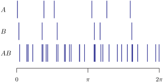
Figure 1: Example spectrum of the direct product of two uncoupled subsystems, Eq. (25), for $N_{A}=N_{B}=6$. The spectra are ordered vertically for subspaces $A$, $B$, and the combined spectrum, respectively. This schematically illustrates two key features, the emergence of Poissonian spacing fluctuations and the great increase in eigenangle density for the combined spectrum.

The associated eigenangles are given by

$$\theta_{jk}=\theta_{j}+\theta_{k}\quad{\rm mod}(2\pi),$$ (25)

see Fig. 1. Note that the mean spacing of eigenangles for $\theta_{j}$ ($\theta_{k}$) is $2\pi/N_{A}$ ($2\pi/N_{B}$), and for $\theta_{jk}$ is $2\pi/N_{A}N_{B}$, showing that the combined spectrum is denser by a factor of either $N_{A}$ or $N_{B}$ than the individual subspace spectra. Choose a particular eigenstate of an ensemble member ($\epsilon\neq 0$), denoted $|\Phi_{jk}\rangle$, as the one which is continuously connected to $|jk\rangle$ as $\epsilon$ vanishes. Its Schmidt decomposition can be written as

$$|\Phi_{jk}\rangle=\sum_{j=1}^{N_{A}}\sqrt{\lambda_{j}}|\phi^{A}_{j}\rangle|\phi^{B}_{j}\rangle,$$ (26)

where $\lambda_{1}\geq\lambda_{2}\geq\cdots\geq\lambda_{N_{A}}$ are the (Schmidt) eigenvalues of the reduced density matrix $\rho^{A}$, and the states $\{|\phi^{A}_{j}\rangle,\;|\phi^{B}_{j}\rangle\}$ are the orthonormal eigenvectors of $\rho^{A}$ and $\rho^{B}$ respectively. The perturbation expression to first order of the eigenstate is (${\cal U}(\epsilon)$ is the member of the ensemble ${\cal U}_{\text{RMT}}(\epsilon)$ under consideration with corresponding $V$)

$$|\Phi_{jk}\rangle\approx|jk\rangle+\epsilon\sum_{j^{\prime}k^{\prime}\neq jk}\dfrac{\langle j^{\prime}k^{\prime}|V|jk\rangle}{\theta_{jk}-\theta_{j^{\prime}k^{\prime}}}\,|j^{\prime}k^{\prime}\rangle\ .$$ (27)

where here and throughout $j^{\prime}k^{\prime}\neq jk$ means to exclude the single term in which both $j^{\prime}=j$ and $k^{\prime}=k$. Note that the eigenbasis $|jk\rangle$ of one member of $U_{A}^{\text{CUE}}\otimes U_{B}^{\text{CUE}}$ is not the one in which the operator $V$ is diagonal, and a transformation to the appropriate eigenbasis must be performed in order to evaluate the matrix elements above. Due to the statistical properties of the ensemble, the transformation between bases is statistically equivalent to choosing a direct product random unitary transformation independently uniform with respect to the Haar measure in each subspace. Thus, there is a central limit theorem for the behavior of the matrix elements. Furthermore, there is a complete absence of correlations between the unperturbed spectra and the unperturbed eigenstates. Like the classical random matrix ensembles, there is an ergodicity Pan1979 for this ensemble as well in that spectral averages taken over an individual member of the ensemble in the large dimensional limit has fluctuation properties that are nearly equal those expected of the ensemble.

An interesting circumstance appears when calculating the density matrix from the perturbation expression, only one row and column have matrix elements of $\mathcal{O}(\epsilon)$,

$$\rho^{A} = |j\rangle\langle j|+\epsilon\sum_{j^{\prime}\neq j}\frac{\langle j^{\prime}k|V|jk\rangle}{\theta_{j}-\theta_{j^{\prime}}}|j^{\prime}\rangle\langle j|+h.c.$$

$$+\epsilon^{2}\sum_{j^{\prime}k^{\prime},j^{\prime\prime}k^{\prime}\neq jk}\dfrac{\langle jk|V|j^{\prime\prime}k^{\prime}\rangle\langle j^{\prime}k^{\prime}|V|jk\rangle}{\left(\theta_{jk}-\theta_{j^{\prime}k^{\prime}}\right)\left(\theta_{jk}-\theta_{j^{\prime\prime}k^{\prime}}\right)}\,|j^{\prime}\rangle\langle j^{\prime\prime}|.$$

However, given the comments above about the statistical nature of the ensemble members, matrix elements vary as zero centered Gaussian random variables without correlation to the energy denominators. In fact, the dominant terms are nearly always those with the smallest energy denominators. The important point is that the eigenangle denominators of the $\mathcal{O}(\epsilon)$ terms involve only the spectrum of subsystem $A$, whose differences are generally a factor $N_{B}$ greater ($N_{B}\geq N_{A}\rightarrow\infty$) than energy denominators involving the full spectrum; recall Fig. 1. So these terms represent an $\mathcal{O}(N_{B}^{-1})$ correction and can be dropped.

Thus, it is necessary to self-consistently track down all the $\mathcal{O}(\epsilon^{2})$ perturbations contributing to the reduced density matrix. It turns out that all the second order terms not shown in Eq. (27) contributing to the summation over the $|jk\rangle$ states contribute at order $\mathcal{O}(\epsilon^{3})$ or greater and can be dropped. The only second order correction that must be accounted for in Eq. (27) is the second order normalization of the $|jk\rangle$ term. Thus, the normalized state with all the terms needed to this order is SakTua1994

$$\begin{split}|\Phi_{jk}\rangle=&\left(1-\frac{\epsilon^{2}}{2}\sum_{j^{\prime}k^{\prime}\neq jk}\dfrac{|\langle jk|V|j^{\prime}k^{\prime}\rangle|^{2}}{(\theta_{jk}-\theta_{j^{\prime}k^{\prime}})^{2}}\right)|jk\rangle\\ &+\epsilon\sum_{j^{\prime}k^{\prime}\neq jk}\dfrac{\langle j^{\prime}k^{\prime}|V|jk\rangle}{\theta_{jk}-\theta_{j^{\prime}k^{\prime}}}|j^{\prime}k^{\prime}\rangle.\end{split}$$ (29)

The expression for the density matrix is finally,

$$\rho^{A} = \left(1-\epsilon^{2}\sum_{j^{\prime}k^{\prime}\neq jk}\dfrac{|\langle jk|V|j^{\prime}k^{\prime}\rangle|^{2}}{(\theta_{jk}-\theta_{j^{\prime}k^{\prime}})^{2}}\right)|j\rangle\langle j|$$

$$+\epsilon^{2}\sum_{j^{\prime}k^{\prime},j^{\prime\prime}k^{\prime}\neq jk}\dfrac{\langle jk|V|j^{\prime\prime}k^{\prime}\rangle\langle j^{\prime}k^{\prime}|V|jk\rangle}{\left(\theta_{jk}-\theta_{j^{\prime}k^{\prime}}\right)\left(\theta_{jk}-\theta_{j^{\prime\prime}k^{\prime}}\right)}\,|j^{\prime}\rangle\langle j^{\prime\prime}|.$$

III.3 Schmidt decomposition

Given the eigenstate expressions for the ensemble, the next step towards evaluating the entanglement entropies is to deduce the Schmidt eigenvalues. A priori, the perturbed state in Eq. (29) is not in the Schmidt decomposed form of Eq. (26) or alternatively, the density matrix expression in Eq. (III.2) has not yet been diagonalized. Therefore it is not yet clear what the reduced density matrix eigenvalues are from the expressions. However, the ensemble of Eq. (23) has some very nice statistical properties, as mentioned in the previous subsection, that greatly simplify the process.

The key argument is that, given the random, featureless interaction (all matrix elements fluctuate about the same scale, independent of the pair of states involved), the dominant terms in perturbation theory come from the nearest neighbors in the spectrum. This has the consequence of inhibiting any changes to the Schmidt eigenvectors. Consider the difference of $\theta_{j+1}-\theta_{j}$, which would result if the value of $k$ is unchanged. It is likely to be much farther away than the nearest neighbors. Much more likely is that an appropriate change in $k$ can help cancel a large part of this difference. For example, $|j+1,k\rangle$ and $|j,k+1\rangle$ has a far greater chance of being nearby as $\theta_{j+1}+\theta_{k}-\theta_{j}-\theta_{k+1}$ has a far greater chance of generating a small difference. In fact, for $N_{A}\rightarrow\infty$ in a local neighborhood of the spectrum, for any given value of $j$, there is only one value of $k$ that has a chance of being close. Similarly, for a given value of $k$, only one value of $j$ has a chance of being close. Thus, the only terms that are appreciable in Eq. (29) lead to mutually orthonormal sets of $\{j,k\}$ locally in the spectrum. The same argument implies that Eq. (III.2) is diagonal as well. Since $j,j^{\prime}$ are matched to the same values of $k$, and a unique value of $j$ gives a near neighbor, one of the diagonal terms will nearly always dominate the $j\neq j^{\prime}$ terms. Thus as a consequence, under these conditions, we have with high probability that the perturbed state in Eq. (29) remains in the Schmidt form to an excellent approximation that gets better with increasing dimensionality. It turns out that corrections to this picture produce higher order corrections after ensemble averaging. Thus, the eigenvalues of the reduced density matrix can be taken directly from the diagonal elements of Eq. (III.2).

III.4 Eigenvalues of the reduced density matrix and ensemble averaging

Following from Eq. (III.2) the expression for the largest eigenvalue $\lambda_{1}$ of the reduced density matrix $\rho^{A}$ is approximately

$$\lambda_{1}\approx 1-\epsilon^{2}\sum_{j^{\prime}k^{\prime}\neq jk}\dfrac{|\langle jk|V|j^{\prime}k^{\prime}\rangle|^{2}}{(\theta_{jk}-\theta_{j^{\prime}k^{\prime}})^{2}}$$ (31)

and the second largest is nearly always

$$\lambda_{2}\approx\epsilon^{2}\dfrac{|\langle jk|V|j_{1}k_{1}\rangle|^{2}}{\left(\theta_{jk}-\theta_{j_{1}k_{1}}\right)^{2}},$$ (32)

where $\theta_{j_{1}k_{1}}$ is the closest eigenangle to $\theta_{jk}$. The dependence of these eigenvalues on the “central state” indices $jk$ is suppressed. To this level of approximation, the largest eigenvalue is simply the squared overlap of the state with its perturbation. Such a situation has been analyzed in the context of parametric eigenstate correlators and the fidelity with a broad variety of physical applications BruLewMuc1996 ; AlhAtt1995 ; AttAlh1995 ; KusMit1996 ; CerTom2003 .

The unperturbed Schmidt vector corresponding to the largest eigenvalue $|j\rangle$ is unchanged in this approximation. This is a statistical approximation that simply reads off the eigenvalues of the reduced density matrix assuming that the significant terms in the perturbation expansion in Eq. (29) are determined by eigenangle denominators and relies on the $|j^{\prime}\rangle$ vectors all being locally orthonormal, and likewise the $|k^{\prime}\rangle$ vectors. A more detailed analysis is possible Lakshminarayan19 that entails constructing the reduced density matrix and making a further perturbation approximation to diagonalize it. This leads to some changes in the formal structure of these expressions. For example, the sum in the largest eigenvalue $\lambda_{1}$ (Eq. (31)) is changed to a more restricted sum such that $j^{\prime}\neq j$ and $k^{\prime}\neq k$. However, these changes only lead to higher order corrections after ensemble averaging and do not affect any of the results presented here.

In order to prepare these expressions for ensemble averaging ahead, it is quite useful to extract certain scales and introduce spectral two-point functions, which can be used to express the summations in integral form FreKotPanTom1988 . First, the statistical properties of the transition matrix elements and the energy differences each involve a single scale. The admixing matrix elements $\epsilon^{2}|\langle jk|V|j^{\prime}k^{\prime}\rangle|^{2}$ in the unperturbed basis behave as the absolute square of a complex Gaussian random variable. Denoting the mean as $v^{2}$, the term $\epsilon^{2}|\langle jk|V|j^{\prime}k^{\prime}\rangle|^{2}$ is replaced by $v^{2}w_{j^{\prime}k^{\prime}}$, where the set of $\{w_{j^{\prime}k^{\prime}}\}$ behave according to the statistical probability density

$$\rho(w)=e^{-w},\;\;w\geq 0,$$ (33)

with unit mean across the ensemble. This is a property of the ensemble, Eq. (23). Note that for a bipartite chaotic dynamical system with the structure of Eq. (2), for which the perturbation is not random, the distribution of $w$ shows deviations from the exponential as illustrated in App. C. Still the predictions of the random matrix ensemble apply very well to the coupled kicked rotors, as will be seen below.

Secondly, the energy denominator has the single scale of a mean spacing, $D=2\pi/(N_{A}N_{B})$, built in. Let $\theta_{jk}-\theta_{j^{\prime}k^{\prime}}=Ds_{j^{\prime}k^{\prime}}$, upon substitution,

$$\lambda_{1}\approx 1-\frac{\epsilon^{2}v^{2}}{D^{2}}\sum_{j^{\prime}k^{\prime}\neq jk}\dfrac{w_{j^{\prime}k^{\prime}}}{s_{j^{\prime}k^{\prime}}^{2}}=1-\Lambda\sum_{j^{\prime}k^{\prime}\neq jk}\dfrac{w_{j^{\prime}k^{\prime}}}{s_{j^{\prime}k^{\prime}}^{2}},$$ (34)

where the second form uses the definition of the transition parameter PanMeh1983 ; FreKotPanTom1988 ,

$$\Lambda=\frac{\epsilon^{2}v^{2}}{D^{2}}.$$ (35)

This illustrates its natural appearance in the perturbation expressions.

Let’s define the function

$$R(s,w)=\sum_{j^{\prime}k^{\prime}\neq jk}\delta\left(w-w_{j^{\prime}k^{\prime}}\right)\delta\left(s-s_{j^{\prime}k^{\prime}}\right).$$ (36)

where $R(s,w)$ is the probability density of finding a level at a rescaled distance $s$ from $\theta_{jk}$, and the corresponding matrix element variable $w$ takes the value $w_{j^{\prime}k^{\prime}}$. In general there could be correlations between matrix elements and spacings, however for the current scenario they are completely independent across the ensemble. Equation (31) can be expressed in an exact integral form using $R(s,w)$ as,

$$\lambda_{1}\approx 1-\Lambda\int^{\infty}_{-\infty}{\rm d}s\int_{0}^{\infty}{\rm d}w\frac{w}{s^{2}}R(s,w).$$ (37)

This expression clarifies a number of issues. First, $\Lambda$ controls the entanglement behavior as asserted in the introduction, and the perturbative regime is for $\Lambda\ll 1$; see Sect. III.5. Another great simplicity is that ensemble averaging of $\lambda_{1}$ is reduced entirely to replacing $R(s,w)$ with its ensemble average, $\overline{R(s,w)}$. For the ensemble of Eq. (23), all correlations between matrix elements and spacing vanish. In fact,

$$\overline{R(s,w)}=\rho(w)R_{2}(s)=\exp(-w),$$ (38)

where the last form follows for the ensemble because $R_{2}(s)=1\ (-\infty\leq s\leq\infty)$ for a Poissonian sequence of unit mean and in general defined as,

$$R_{2}(s)=\overline{\sum_{j^{\prime}k^{\prime}\neq jk}\delta\left(s-s_{j^{\prime}k^{\prime}}\right)}.$$ (39)

The eigenangles are pairwise sums of those with CUE fluctuations. These lose correlations and are Poisson distributed. For a recent rigorous mathematical proof in the context of product unitary operators see TkoSmaKusZeiZyc2012 . Another issue is that of calculating moments of the Schmidt eigenvalues, which is treated in Sect. IV. We only mention here that the moments involve more complicated expressions than are given in Eq. (38). Finally, the spacing integral in Eq. (37) using Eq. (38) for ensemble averaging leads to a divergence which requires a regularization as there are too many small spacings. The regularization is given in Sect. III.6.

A curious feature arises for the ensemble averaging of the expression for $\lambda_{2}$. The expression for the nearest neighbor spacing density of a Poissonian sequence arises from the consideration of consecutive spacings between eigenvalues. However, $|j_{1}k_{1}\rangle$ is selected to be the closest nearest neighbor. In effect, $\theta_{jk}$ has a nearest neighbor to the left and one to the right in the spectrum, and $|j_{1}k_{1}\rangle$ is determined by the smaller spacing of the two. The standard result $\rho_{\text{NN}}(s)=\exp(-s)$ is not the appropriate density. Rather, the closer neighbor density, $\rho_{\text{CN}}(s)$, is given by

$$\rho_{\text{CN}}(s)=2\exp(-2s)\ \ (0\leq s\leq\infty)$$ (40)

for a Poissonian spectrum of unit mean spacing LakSriKetBaeTom2016 ; OurRNNS .

Collecting results gives

$$\overline{\lambda_{1}} \approx 1-\Lambda\int^{\infty}_{-\infty}{\rm d}s\int_{0}^{\infty}{\rm d}w\frac{w}{s^{2}}e^{-w}$$ (41a)

$$\overline{\lambda_{2}} \approx 2\Lambda\int_{0}^{\infty}\frac{w}{s^{2}}e^{-w-2s}\,dw\,ds.$$ (41b)

As mentioned earlier for $\lambda_{1}$, both equations (41) diverge as $s\rightarrow 0$. The divergence indicates that the correct order of $\overline{\lambda_{1}}$ or $\overline{\lambda_{2}}$ is not, in fact, $1-\mathcal{O}(\Lambda)$ or $\mathcal{O}(\Lambda)$, respectively. Instead, they turn out to be of the form $\overline{\lambda_{1}}=1-\mathcal{O}(\sqrt{\Lambda})$ and $\overline{\lambda_{2}}=\mathcal{O}(\sqrt{\Lambda})$, and indeed the average of the general moments in Eq. (7) for $\alpha>1/2$ differ from $1$ by terms of the $\mathcal{O}(\sqrt{\Lambda})$, as shown in Sect. IV. Thus the eigenvalues and moments are much more “volatile” than suggested by naive perturbation theory. This will be further related in Sect. V to the emergence of power laws in the probability density of reduced density matrix eigenvalues in this regime.

III.5 The transition parameter $\Lambda$

Once the universal transition curve is derived for the random matrix ensemble (23), it is of interest to explore how well the universal results apply to chaotic dynamical systems. For that reason, instead of deriving the expression for $\Lambda$ exclusively for the ensemble of Eq. (23), a slightly more general expression is derived. The subsystem unitary operators are taken from the CUE (imitated well by the chaotic dynamical subsystems), but the interaction is left unspecified allowing for greater flexibility and generality of applicability. It turns out that the transition parameter expression under such circumstances is given by (see App. B for a detailed derivation)

$$\begin{split}&\Lambda=\dfrac{N_{A}^{3}N_{B}^{3}}{4\pi^{2}(N_{A}^{2}-1)(N_{B}^{2}-1)}\times\\ &\left(1+\left|\frac{\text{tr}U_{AB}}{N_{A}N_{B}}\right|^{2}-\frac{1}{N_{A}}\,\left\|\frac{U^{(A)}}{N_{B}}\right\|^{2}-\frac{1}{N_{B}}\,\left\|\frac{U^{(B)}}{N_{A}}\right\|^{2}\right).\end{split}$$ (42)

Here $U^{(A)}_{ii}=\sum_{k}(U(\epsilon))_{ik}$, $U^{(B)}_{kk}=\sum_{i}(U(\epsilon))_{ik}$ are partially traced (still diagonal) interaction operators, which are in general not unitary, and $\|X\|^{2}=\text{Tr}(XX^{\dagger})$ is the Hilbert-Schmidt norm. It can be checked that this $\Lambda$ correctly vanishes if $V$ is a function of either coordinate alone, and thereby not entangling. However, it does not vanish for general separable potentials, and hence the assumption that the interaction is entangling is necessary. Equation (42) is the generalization of the corresponding result stated in Ref. SriTomLakKetBae2016 for the case $N_{A}=N_{B}=N$.

Performing an additional ensemble average over the diagonal random phases for the $U(\epsilon)$ of Eq. (23) gives

$$\begin{split}\Lambda_{\text{RMT}}&=\dfrac{N_{A}^{2}N_{B}^{2}}{4\pi^{2}(N_{A}+1)(N_{B}+1)}\left[1-\dfrac{\sin^{2}(\pi\epsilon)}{\pi^{2}\epsilon^{2}}\right]\\ &\approx\dfrac{N_{A}N_{B}\epsilon^{2}}{12},\end{split}$$ (43)

where for the last expression the limits $N_{A},N_{B}\gg 1$ and $\epsilon\ll 1$ have been used. Equation (43) clearly demonstrates the sensitivity of a large system to even extraordinarily weak coupling. Only if $N_{A},N_{B}$, and $\epsilon$ are scaled such that $\Lambda_{\text{RMT}}$ is kept fixed, universal statistical behavior of the bipartite system is to be expected. In contrast, without fixing the scaling of $\Lambda$, as $N_{A}\rightarrow\infty$, the transition to effectively random eigenstates would be discontinuously rapid if $\epsilon>0$.

The evaluation of $\Lambda$ generally is much more complicated in many-body systems; see FreKotPanTom1988b where it was analyzed for the compound nucleus in the context of time reversal symmetry breaking. One extremely important factor complicating the analysis in most cases is that no matter how many particles are involved in the system, their interactions are dominated or limited to one- and two-body operators. In the standard random matrix ensembles, if they are being used to model a system of $m$-particles, the ensemble implicitly is dominated by $m$-body interactions. If not, there would have to be a large number of matrix elements put to zero in an appropriate basis of Slater determinant states. This fact has led to the study of the more complicated and difficult to work with so-called embedded ensembles Kot2014 . In fact, as the number of particles increases, Hamiltonian matrix elements would become increasingly sparse. The selection rules arising through the restriction of the body rank of the interactions thus create a great deal of matrix element correlations and large scale structure imposed on local fluctuations. For the nuclear time reversal breaking analysis, it was possible to cast the theory as a means to calculate an effective dimensionality, which is necessarily much smaller than the dimensionality of the full space.

III.6 Regularization of perturbation theory

The main approach to regularize the divergences that arise in the perturbation theory of symmetry breaking random matrix ensembles was introduced in the earliest works on the subject FreKotPanTom1988 ; Tom1986 . There sometimes arises fluctuation measure specific or symmetry specific aspects, but the basic approach is common to all cases. Typically, the leading order is determined by the regularization required for a pair of levels (eigenphases) to become nearly degenerate. The probability of three or more levels is sufficiently lower as to generate only higher order corrections.

Consider one realization with a pair of levels that are nearly degenerate and sufficiently isolated. There is a subset, yet still infinite, series of terms in the perturbation theory that contains the near vanishing denominators responsible for the divergence. Isolating just that series of terms, they have to be equivalent to the series arising from a two-level system. Thus, regularization to lowest order proceeds by using the two level exact solution to represent the resummation of this infinite series of diverging terms. The effective and scaled Hamiltonian, ignoring an irrelevant phase, is

$$\left(\begin{array}[]{cc}s/2&\sqrt{\Lambda w}\\ \sqrt{\Lambda w}&-s/2\end{array}\right),$$ (44)

where the $jk$ subscript is suppressed on $s$ and $w$. The unperturbed state $(1,0)^{T}$ gets rotated by the interaction $\Lambda>0$ to $(1,a)^{T}/\sqrt{1+|a|^{2}}$, where

$$|a|^{2}=\dfrac{\left(s-\sqrt{s^{2}+4\Lambda w}\right)^{2}}{4\Lambda w}=\dfrac{4\Lambda w}{(s+\sqrt{s^{2}+4\Lambda w})^{2}}.$$ (45)

The weight $\Lambda w/s^{2}$ of the mixing as obtained by perturbation theory, is replaced by $|a|^{2}/(1+|a|^{2})$, i.e. with a bit of algebra the regularization is seen to involve the replacement

$$\dfrac{\Lambda w}{s^{2}}\mapsto\dfrac{1}{2}\left(1-\dfrac{|s|}{\sqrt{s^{2}+4\Lambda w}}\right).$$ (46)

This correctly accounts for near degenerate cases when $s\rightarrow 0$ and the states are nearly equally superposed. For larger $s$, in the perturbative regime that we are interested in, $\Lambda\ll 1$, the mapping is effectively accounting for a part of the higher order corrections. It does no harm to use the regularized expression beyond where it is needed as it only effects higher order corrections. Such a regularization is better substantiated and more accurate than providing simply a lower cut-off to divergent integrals in the spacing $s$.

Making this substitution in Eq. (41) gives the expectation values of the first two Schmidt eigenvalues as

$$\overline{\lambda_{1}} \approx 1-\int^{\infty}_{0}{\rm d}s\int_{0}^{\infty}{\rm d}w\left(1-\dfrac{s}{\sqrt{s^{2}+4\Lambda w}}\right)e^{-w}$$ (47)

$$= 1-\sqrt{\pi\Lambda}$$

$$\overline{\lambda_{2}} \approx \int^{\infty}_{0}{\rm d}s\int_{0}^{\infty}{\rm d}w\left(1-\dfrac{s}{\sqrt{s^{2}+4\Lambda w}}\right)e^{-w-2s}$$ (48)

$$= \sqrt{\pi\Lambda}+2e^{-4\Lambda}\Lambda\left(\text{Ei}(4\Lambda)-\pi\text{erfi}\left(2\sqrt{\Lambda}\right)\right)$$

$$= \sqrt{\pi\Lambda}+2\Lambda[\gamma+\ln(4\Lambda)]-8\sqrt{\pi}\Lambda^{3/2}+...\ ,$$ (49)

where the imaginary error function is $\text{erfi}(x)=-\text{i}\text{erf}(\text{i}x)$, $\text{Ei}(x)$ is the exponential integral (DLMF, , Eq. 6.2.5), and $\gamma=0.57721...$ is Euler’s constant. The last line gives the functional expansion for the small $\Lambda$ regime, a bit beyond the $\Lambda$-order to which it is valid.

As mentioned previously, the lowest order behavior is augmented from $\Lambda$ to $\sqrt{\Lambda}$ once the divergence is regularized properly. It also turns out that $\overline{\lambda_{1}}+\overline{\lambda_{2}}=1+\mathcal{O}(\Lambda\ln\Lambda)$. The third and smaller Schmidt eigenvalues must contribute in higher orders of the transition parameter. This fact is crucial for the development of the recursively embedded perturbation theory in Sect. VI.

III.7 A Floquet system: coupled kicked rotors

It is instructive to have a simple, bipartite, deterministic, chaotic dynamical system to compare against the universal transition results emerging from random matrix theory for the rest of the paper. Simple in this context means that it is possible both to calculate the value of $\Lambda$ as a function of interaction strength analytically, and to carry out calculations for reasonably large values of $N_{A},N_{B}$. A system of two coupled kicked rotors quantized on the unit torus is ideal. Here we will restrict the numerical computations to the case $N_{A}=N_{B}=N$.

A rather general class of interacting bipartite systems can be described by the unitary Floquet operator of the form given in Eq. (2), including many-body systems. A specific example, leading to the kicked rotors, for which the quantum time-evolution operator has this form begins with the Hamiltonian

$$\begin{split}H=&\frac{1}{2}(p_{A}^{2}+p_{B}^{2})\\ &+\bigl{[}V_{A}(q_{A})+V_{B}(q_{B})+b\,V_{AB}(q_{A},q_{B})\bigr{]}\,\delta_{t}\end{split}$$ (50)

where $\delta_{t}=\sum_{n=-\infty}^{\infty}\delta(t-n)$ is a periodic sequence of kicks with unit time as the kicking period. The subsystem one-kick unitary propagators connecting states are given by

$$U_{A}=\exp[-\text{i}p_{A}^{2}/(2\hbar)]\exp(-\text{i}V_{A}/\hbar)$$ (51)

and likewise for $B$. The interaction or entangling operator is

$$U_{AB}(b)=\exp(-ibV_{AB}/\hbar).$$ (52)

The classical system is well defined and given by a $4$-dimensional symplectic map with the interaction strength tuned by the parameter $b$. A particularly important and well studied example are the coupled kicked rotors Fro1971 ; Fro1972 , which have been realized in experiments on cold atoms GadReeKriSch2013 . The most elementary case is for two interacting rotors with the single particle potentials

$$V_{A}=K_{A}\cos(2\pi q_{A})/4\pi^{2}$$ (53)

similarly for $B$, and the coupling interaction

$$V_{AB}=\frac{1}{4\pi^{2}}\,\cos[2\pi(q_{A}+q_{B})].$$ (54)

The unit periodicity in the angle variables $q_{j}$ is extended here to the momenta $p_{j}$ so that the phase space is a 4-dimensional torus.

If the kicking strengths $K_{A}$ and $K_{B}$ of the individual maps are each chosen sufficiently large, the maps in $(q_{A},p_{A})$ and $(q_{B},p_{B})$ are strongly chaotic with a Lyapunov exponent of approximately $\ln(K/2)$ Chi1979 . There are some special ranges of $K$ to avoid corresponding to small scale islands formed by the so-called accelerator modes Chi1979 . This is supported by recent rigorous results showing that the stochastic sea of the standard map has full Hausdorff dimension for sufficiently large generic parameters Gor2012 . In this article $K_{A}=10$ and $K_{B}=9$ are used everywhere in which case the dynamics of the uncoupled maps numerically is sufficiently chaotic, i.e. no regular islands exist on a scale large enough to matter.

The quantum mechanics on a torus phase space of a single rotor leads to a finite Hilbert space of dimension $N$, see e.g. Refs. BerBalTabVor1979 ; HanBer1980 ; ChaShi1986 ; KeaMezRob1999 ; DegGra2003bwcrossref . The effective Planck constant is $h=1/N$. Thus $U_{A}$ and $U_{B}$ are $N$–dimensional unitary operators on their respective spaces. Explicitly, the unitary matrix $U_{A}$ reads

$$U_{A}(n^{\prime},n)\,=\,\frac{1}{N}\,\exp\left(-iN\frac{K_{A}}{2\pi}\cos\left(\frac{2\pi}{N}(n+\theta_{p})\right)\right)$$

$$\times\,\sum_{m=0}^{N-1}\exp\left(-\frac{\pi i}{N}(m+\theta_{q})^{2}\right)\,\exp\left(\frac{2\pi i}{N}(m+\theta_{q})(n-n^{\prime})\right).$$ (55)

where $n,n^{\prime}\in\{0,1,...,N-1\}$. The parameters $\theta_{q},\theta_{p}\in[0,1[$ allow for shifting the position grid by which any present symmetries, in particular parity and time-reversal, can be broken.

If $U_{AB}(b)$ is only a function of position, such as in Eq. (50), this can be represented in position space by a diagonal matrix. Thus, the resulting $N^{2}\times N^{2}$–dimensional unitary matrix for the coupled kicked rotors is given by

$$\langle n_{1}^{\prime}n_{2}^{\prime}|{\cal U}_{\text{KR}}|n_{1}n_{2}\rangle\,=\,U_{A}(n_{1}^{\prime},n_{1})\,U_{B}(n_{2}^{\prime},n_{2})\,$$

$$\times\exp\left(-iN\frac{b}{2\pi}\cos(\frac{2\pi}{N}(n_{1}+n_{2}+2\theta_{p}))\right).$$ (56)

The choice $N=100$ is taken as sufficiently large to give asymptotic results and the phases $\theta_{q}=0.34$ and $\theta_{p}=0.24$ are chosen to break time-reversal and parity symmetry, respectively. Such coupled quantum maps have been studied in different contexts Lak2001 ; RicLanBaeKet2014 where more details can be found. Note that coupled kicked rotors with a different interaction term have also been studied on the cylinder She1994 .

Applying Eq. (42) to the coupled kicked rotors gives

$$\Lambda_{\text{KR}}=\frac{N^{2}}{4\pi^{2}}\left(1-J_{0}^{2}(Nb/2\pi)\right)\approx\frac{N^{4}b^{2}}{32\pi^{4}},$$ (57)

where the approximation holds for $Nb\ll 1$. Using the approximations in Eqs. (43) and (57) relates the kicked rotor interaction strength $b$ to the parameter $\varepsilon$ of the random matrix model explicitly, i.e.

$$\epsilon=\sqrt{\frac{3}{8\pi^{4}}}\,Nb,$$ (58)

for small values of $\epsilon$ and $Nb$, and $N\gg 1$. In practice this approximation is good for the entire transition even if $N$ is only moderately large.

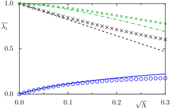
Figure 2: Average Schmidt eigenvalues $\overline{\lambda_{1}}$ (black crosses) and $\overline{\lambda_{2}}$ (blue circles) and their sum (green squares) for the coupled kicked rotors versus $\sqrt{\Lambda}$. Comparison with the corresponding predictions (47), dashed black line, (48), full blue curve, and their sum, dashed-dotted green curve.

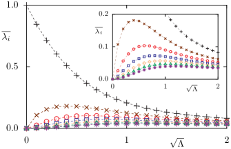
Figure 3: Average Schmidt eigenvalues $\overline{\lambda_{i}}$, $i=1,2,...,7$, (symbols with lines as guide to the eye, from top to bottom) for the coupled kicked rotors versus $\sqrt{\Lambda}$.

Let us first compare the first two mean Schmidt eigenvalues of the coupled kicked rotors to the random matrix ensemble predictions, see Fig. 2. The averaging is a spectral average over all $N^{2}$ eigenstates for the coupled kicked rotors. The perturbative nature of the expression Eq. (47) for $\overline{\lambda_{1}}$ is evident showing that the derivation only provides the initial dependence at $\Lambda=0$ as it is designed to do. For $\overline{\lambda_{2}}$ the validity of the result (48) extends beyond the initial dependence as given by Eq. (49).

IV Eigenvalue moments of the reduced density matrix

For a global view of the spectrum of the reduced density matrix as the coupling is increased, Fig. 3 shows the behavior of various $\overline{\lambda_{i}}$ versus $\sqrt{\Lambda}$. Here, and in the following we restrict to $N_{A}=N_{B}=N$ with $N=100$ chosen for the numerical computations. It is seen from the figure that whereas $\overline{\lambda_{1}}$ monotonically decreases towards its random matrix average of $\approx 4/N$, other principal eigenvalues, such as the second or third largest, display a non-monotonic approach to their respective averages. The smallest eigenvalue, $\overline{\lambda_{N}}$ grows to about $1/N^{3}$, which is the random matrix average Zni2007 ; MajBohLak2008 . For $\Lambda\gg 1$, the probability density of the set of $\lambda_{i}$ follows the Marčenko-Pastur distribution given in Eq. (9). The largest alone is distributed according to the Tracy-Widom density (after appropriate scaling and shift) TraWid1996 , whereas the smallest is known to be exponential MajBohLak2008 . Numerical results for the transition towards these results are presented in Sect. V. Also see the recent paper KumSamAna2017 for additional random matrix results concerning the smallest eigenvalue and applications to coupled kicked tops.

IV.1 General moments

To characterize the entanglement in bipartite systems the general moments $\mu_{\alpha}$ of Eq. (7) and thus the sum of the averages $\overline{\lambda_{j}^{\alpha}}$ are needed. The relationship of the entropies to the general moments is given in Eq. (8). In the perturbative regime, the largest eigenvalue $\lambda_{1}$ decreases from 1, see Fig. 2, and thus has a different behavior compared to all other eigenvalues. This is clear from the content of Eqs. (31) and (32) where each eigenvalue $\lambda_{j}$ with $j>1$ has its own expression, while the largest follows from normalization, $\lambda_{1}=1-\sum_{j>1}\lambda_{j}$. Therefore it is necessary to treat the general moments of $\lambda_{1}$ separately from the others as it requires some additional analysis.

IV.1.1 Moments $\sum_{j>1}\lambda_{j}^{\alpha}$

The moment expressions for the $\sum_{j>1}\lambda_{j}^{\alpha}$ can be written down immediately from the results of Sects. III.4, III.6. There is no need to invoke the closer next neighbor statistics as there is a sum over all the eigenvalues $j>1$ of the unperturbed Hamiltonian and hence $R_{2}(s)=1$. This gives for the $\alpha$ ($>1/2$) moment

$$\sum_{j>1}\overline{\lambda_{j}^{\alpha}}=$$ (59)

$$\int^{\infty}_{-\infty}{\rm d}s\int_{0}^{\infty}\frac{{\rm d}w}{2^{\alpha}}\left(1-\dfrac{|s|}{\sqrt{s^{2}+4\Lambda w}}\right)^{\alpha}\overline{R(s,w)}$$

$$= \int^{\infty}_{-\infty}{\rm d}s\int_{0}^{\infty}\frac{{\rm d}w}{2^{\alpha}}\left(1-\dfrac{|s|}{\sqrt{s^{2}+4\Lambda w}}\right)^{\alpha}e^{-w}$$

$$= C_{2}(\alpha)\sqrt{\Lambda}$$

where

$$\begin{split}C_{2}(\alpha)&=2\sqrt{\pi}\int_{0}^{\pi/2}\dfrac{1}{\sin^{2}\theta}\sin^{2\alpha}\frac{\theta}{2}\,d\theta\\ &=\dfrac{\sqrt{\pi}}{2}\int_{0}^{1/2}\dfrac{t^{\alpha}}{t^{3/2}(1-t)^{3/2}}dt\\ &=\dfrac{\sqrt{\pi}}{2}\text{B}_{1/2}\left(\alpha-\frac{1}{2},-\frac{1}{2}\right),\;\;\alpha>1/2.\end{split}$$ (60)

Here $B_{z}(a,b)$ is the incomplete Beta function (DLMF, , Eq. 8.17.1) defined as

$$\begin{split}B_{z}(a,b)&=\int_{0}^{z}t^{a-1}(1-t)^{b-1}\,dt\\ &=\frac{z^{a}}{a}\;_{2}F_{1}\left(a,1-b;a+1;x\right).\end{split}$$ (61)

Note that the evaluation of the integral is exact and that all moments ($\alpha>1/2$) are proportional to $\sqrt{\Lambda}$, i.e. there are no higher order terms coming from these expressions. If $\alpha=1/2$ there is a divergence ($C_{2}(1/2)=\infty$) and this is a special value as far as the moments are concerned. This is due to the contributions of the very small eigenvalues. It turns out that for $\alpha=1/2$ the order is no longer $\sqrt{\Lambda}$. This will be dealt with later in Sect. IV.3.

The result for $\alpha=1$, which follows from $C_{2}(1)=\sqrt{\pi}$, is identical to the leading order of the average second largest eigenvalue in Eq. (49). The reason for this is that the other eigenvalues do not contribute to this order. This really justifies the use of only two reduced density matrix eigenvalues in the perturbative regime. Another special case corresponding to $\alpha=2$ gives

$$\sum_{j>1}\overline{\lambda_{j}^{2}}=\sqrt{\pi\Lambda}\,(1-\pi/4).$$ (62)

IV.1.2 Moments of $\lambda_{1}$

Turning to the largest eigenvalue, it is given by

$$\overline{\lambda_{1}^{\alpha}}=\overline{\left(1-\sum_{j>1}\lambda_{j}\right)^{\alpha}}$$

$$=\overline{\left(1-\int^{\infty}_{-\infty}{\rm d}s\int_{0}^{\infty}\frac{{\rm d}w}{2}\left(1-\dfrac{|s|}{\sqrt{s^{2}+4\Lambda w}}\right)R_{2}(s,w)\right)^{\alpha}}.$$

The extra ingredient not present for the moments of the other eigenvalues is the ensemble averaging of the powers of the density, $R(s,w)$, are also involved. To see how this changes the moment calculations, consider the simplest case, the quadratic terms in the binomial expansions of the moments. There is a quadruple integral for which one needs the ensemble average of $R(s_{1},w_{1})R(s_{2},w_{2})$. It has two contributions, those coming from off-diagonal terms in the products of $\delta$-functions from Eq. (36) and the diagonal terms. Thus,

$$\overline{R(s,w)R(s^{\prime},w^{\prime})}$$ (64)

$$= \rho(w)\rho(w^{\prime})R_{3}(s,s^{\prime})+\delta\left(w-w^{\prime}\right)\rho(w)\delta\left(s-s^{\prime}\right)R_{2}(s)$$

$$= e^{-w-w^{\prime}}+\delta\left(s-s^{\prime}\right)\delta\left(w-w^{\prime}\right)e^{-w}.$$

The second line follows due to the independence of the matrix elements from each other and the spectrum, and the fact that it is the three-point correlation function of the spectrum that enters. Fortunately, for Poisson sequences, for all $k$, $R_{k}=1$, and that gives the last line.

The second moment therefore is given by

$$\overline{\lambda_{1}^{2}} = 1-2\int^{\infty}_{-\infty}{\rm d}s\int_{0}^{\infty}\frac{{\rm d}w}{2}\left(1-\dfrac{|s|}{\sqrt{s^{2}+4\Lambda w}}\right)e^{-w}+$$ (65)

$$\int^{\infty}_{-\infty}{\rm d}s\int_{0}^{\infty}\frac{{\rm d}w}{4}\left(1-\dfrac{|s|}{\sqrt{s^{2}+4\Lambda w}}\right)^{2}e^{-w}+$$

$$\left[\int^{\infty}_{-\infty}{\rm d}s\int_{0}^{\infty}\frac{{\rm d}w}{2}\left(1-\dfrac{|s|}{\sqrt{s^{2}+4\Lambda w}}\right)e^{-w}\right]^{2}$$

$$= 1-2C_{2}(1)\sqrt{\Lambda}+C_{2}(2)\sqrt{\Lambda}+C_{2}^{2}(1)\Lambda$$

$$= 1-\left(1+\frac{\pi}{4}\right)\sqrt{\pi\Lambda}+\pi\Lambda.$$

It is immediately apparent that the leading order terms proportional to $\sqrt{\Lambda}$ come from the diagonal terms for which all the energy and matrix element variables are reduced to the mimimum set. Note that there is only one way for all the variables to be maximally correlated; i.e. the sets of integration variables $\{w_{j}\},\{s_{j}\}$ reduce to $(w,s)$. There are corrections, depending on the moment $\alpha$ considered, polynomial in $\sqrt{\Lambda}$. The next to leading order, $\mathcal{O}(\Lambda)$, come from terms whose integrals can be reduced to $(w_{1},w_{2},s_{1},s_{2})$. In the second moment example shown above, there is only one term that is of this form. However, for arbitrary moments, there are a variety of combinations of possibilities that form a sub-binomial expansion given ahead.

IV.1.3 The leading order of $\lambda_{1}$ moments

Beginning with the binomial expansion of the moments, the leading order comes from the terms remaining after reducing the power of summations to a single summation

$$\overline{\lambda_{1}^{\alpha}} = \overline{\left(1-\sum_{j>1}\lambda_{j}\right)^{\alpha}}$$ (66)

$$= \overline{\left(\sum_{k=0}^{\infty}-1^{k}\left(\alpha\atop k\right)\left[\sum_{j>1}\lambda_{j}\right]^{k}\right)}$$

$$\mapsto \overline{\left(\sum_{k=0}^{\infty}-1^{k}\left(\alpha\atop k\right)\sum_{j>1}\lambda_{j}^{k}\right)}.$$

By inverting the order of the remaining summations, the series can be resummed to give a compact expression for arbitrary moments. The zero^th order terms have to be handled separately. This gives,

$$\overline{\lambda_{1}^{\alpha}} = \overline{1+\sum_{j>1}\sum_{k=1}^{\infty}-1^{k}\left(\alpha\atop k\right)\lambda_{j}^{k}}$$ (67)

$$= \overline{1+\sum_{j>1}\left[\left(1-\lambda_{j}\right)^{\alpha}-1\right]}$$

$$= 1-C_{1}(\alpha)\sqrt{\Lambda},$$

where

$$\begin{split}C_{1}(\alpha)&=2\sqrt{\pi}\int_{0}^{\pi/2}\frac{1}{\sin^{2}\theta}\left(1-\cos^{2\alpha}\frac{\theta}{2}\right)\,d\theta\\ &=\frac{\sqrt{\pi}}{2}\int_{0}^{1/2}\frac{1-(1-t)^{\alpha}}{t^{3/2}(1-t)^{3/2}}dt\\ &=\sqrt{2\pi}\;_{2}F_{1}\left(-\frac{1}{2},\frac{3}{2}-\alpha;\frac{1}{2};\frac{1}{2}\right).\end{split}$$ (68)

Here ${}_{2}F_{1}(\cdot)$ is the Gauss hypergeometric function (DLMF, , Eq. 15.2.1) defined as

$${}_{2}F_{1}\left(a,b;c;z\right)=1+\frac{a\,b}{1!\,c}z+\frac{a(a+1)\,b(b+1)}{2!\,c(c+1)}z^{2}+\cdots.$$

With the analytic results for $C_{1}(\alpha)$ and $C_{2}(\alpha)$, the results of Eq. (49) have been generalized to complete general moments. $C_{1}(1)=\sqrt{\pi}$ is consistent with the expression given there, and $C_{1}(2)=1+\tfrac{\pi}{4}$ is consistent with Eq. (65). A moment of special interest ahead is

$$\overline{\sqrt{\lambda_{1}}}=1-\sqrt{\pi\Lambda}\,[\sqrt{2}-\ln(1+\sqrt{2})],$$ (69)

due to its relationship to the nearest maximally entangled state.

IV.1.4 The $\mathcal{O}(\Lambda)$ correction of the $\lambda_{1}$ moments

In order to calculate the $\mathcal{O}(\Lambda)$ correction of the $\lambda_{1}$ moments, the key question is the combinatoric one of separating the eigenvalues in each term of $\left[\sum_{j>1}\lambda_{j}\right]^{k}$ into two groups; of course, $k\geq 2$. The results is

$$\left[\sum_{j>1}\lambda_{j}\right]^{k} \mapsto \frac{1}{2}\sum_{l=1}^{k-1}\left(k\atop l\right)\sum_{j>1}\sum_{j^{\prime}>1\neq j}\lambda_{j}^{l}\lambda_{j^{\prime}}^{k-l}$$

$$= \frac{1}{2}\sum_{j>1}\sum_{j^{\prime}>1\neq j}\sum_{l=1}^{k-1}\left(k\atop l\right)\lambda_{j}^{l}\lambda_{j^{\prime}}^{k-l}$$

$$= \frac{1}{2}\sum_{j>1}\sum_{j^{\prime}>1\neq j}\left[\left(\lambda_{j}+\lambda_{j^{\prime}}\right)^{k}-\lambda_{j}^{k}-\lambda_{j^{\prime}}^{k}\right].$$

Therefore, the $\mathcal{O}(\Lambda)$ correction $C_{3}(\alpha)\Lambda$ is given by

$$C_{3}(\alpha)\Lambda=$$

$$\frac{1}{2}\sum_{j>1}\sum_{j^{\prime}>1\neq j}\overline{\left(\sum_{k=2}^{\infty}-1^{k}\left(\alpha\atop k\right)\left[\left(\lambda_{j}+\lambda_{j^{\prime}}\right)^{k}-\lambda_{j}^{k}-\lambda_{j^{\prime}}^{k}\right]\right)}$$

$$=\frac{1}{2}\sum_{j>1}\sum_{{j^{\prime}>1}\atop\neq j}\overline{1+\left(1-\lambda_{j}-\lambda_{j^{\prime}}\right)^{\alpha}-\left(1-\lambda_{j}\right)^{\alpha}-\left(1-\lambda_{j^{\prime}}\right)^{\alpha}},$$

which after using the same manipulations as for the earlier integrals leads to

$$C_{3}(\alpha)=\frac{\pi}{8}\int_{0}^{1/2}{\rm d}t_{1}\int_{0}^{1/2}{\rm d}t_{2}\times$$

$$\frac{\left[1+(1-t_{1}-t_{2})^{\alpha}-(1-t_{1})^{\alpha}-(1-t_{2})^{\alpha}\right]}{t_{1}^{3/2}(1-t_{1})^{3/2}t_{2}^{3/2}(1-t_{2})^{3/2}}.$$ (72)

Note that $C_{3}(2)=\pi$, which is consistent with Eq. (65). For some other values of $\alpha$ relevant in the following, the integral evaluates to $C_{3}(3)=\frac{3\pi^{2}}{4}$ and $C_{3}(4)=2\pi+\frac{3\pi^{3}}{16}$. The computations of $\overline{\lambda_{1}^{2}}$, $\overline{\lambda_{1}^{1/2}}$, and $\sum_{j>1}\overline{\lambda_{j}^{2}}$ for the coupled kicked rotors are shown in Fig. 4 and compared to the analytic results of Eqs. (65) and (69), and Eq. (62), respectively. The agreement in the perturbative regime is quite good.

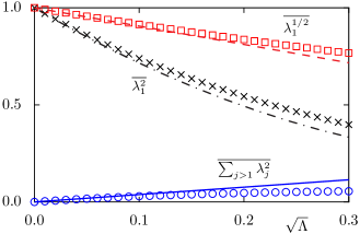
Figure 4: Average moments $\overline{\lambda_{1}^{2}}$ (black crosses), $\overline{\lambda_{1}^{1/2}}$ (red squares), and $\sum_{j>1}\overline{\lambda_{j}^{2}}$ (blue circles) for the coupled kicked rotors versus $\sqrt{\Lambda}$. These are compared to their corresponding perturbative results, Eq. (65), dashed-dotted line, Eq. (69), dashed red line, and Eq. (62), full blue line, respectively.

IV.2 Entropies

With these results for the average eigenvalue moments of the reduced density matrix, everything needed for the entropies defined in Eq. (7) has been evaluated. Combining Eq. (62) with Eq. (65) results in

$$\overline{\mu_{2}}=\sum_{j=1}^{N}\overline{\lambda_{j}^{2}}=\overline{\text{tr}({\rho^{A}}^{2})}=1-\frac{\pi^{3/2}}{2}\sqrt{\Lambda}+\pi\Lambda,$$ (73)

where the neglected terms are presumably of $\mathcal{O}(\Lambda^{3/2})$. This is the random matrix prediction for the purity of the density matrix of generic eigenstates of chaotic subsystems that are perturbatively entangled due to the coupling. As decoherence, i.e. coupling of a system to the environment is usually the cause of loss of purity, this shows the universal manner in which “decoherence” due to coupling with a chaotic subsystem results in the degradation of the purity of eigenstates.

The generalized moments for $\alpha>1/2$ are

$$\overline{\mu_{\alpha}}=\sum_{j=1}^{N}\overline{\lambda_{j}^{\alpha}}=1-C(\alpha)\sqrt{\Lambda}+C_{3}(\alpha)\Lambda+...$$ (74)

where

$$\begin{split}C(\alpha)&=C_{1}(\alpha)-C_{2}(\alpha)=\frac{\sqrt{\pi}}{4}\int_{0}^{1}\dfrac{1-t^{\alpha}-(1-t)^{\alpha}}{t^{3/2}(1-t)^{3/2}}dt\\ &=\pi\frac{\Gamma(\alpha-\nicefrac{{1}}{{2}})}{\Gamma(\alpha-1)}.\end{split}$$ (75)

The incomplete Beta functions of $C_{1}(\alpha)$ and $C_{2}(\alpha)$ combine to produce complete Beta functions. This perturbative moment evaluation is one of the central results of this work. Note that $C(1)=C_{3}(0)=0$, correctly reproducing the unit trace of the density matrix, and that $C(\alpha)<0$ for $\alpha<1$. In the regime when $\alpha<1$ the smaller eigenvalues start to become more important as well. The critical value $\alpha=1$ corresponds to the von Neumann entropy and is of central interest in quantum information.

Thus it follows that the average HCT entropies, defined in Eq. (8), for small $\Lambda$ are

$$\overline{S_{\alpha}}=\pi\frac{\Gamma(\alpha-1/2)}{\Gamma(\alpha)}\sqrt{\Lambda}-\frac{C_{3}(\alpha)}{\alpha-1}\Lambda.$$ (76)

and the $\lim_{\alpha\rightarrow 1}C_{3}(\alpha)/(\alpha-1)=C_{3\text{L}}(1)$ is the integral

$$C_{3\text{L}}(1) =\frac{\pi}{8}\int_{0}^{1/2}\int_{0}^{1/2}\frac{{\rm d}t_{1}{\rm d}t_{2}}{t_{1}^{3/2}(1-t_{1})^{3/2}t_{2}^{3/2}(1-t_{2})^{3/2}}\times$$ (77)

$$\qquad\left[(1-t_{1}-t_{2})\ln(1-t_{1}-t_{2})\right.$$

$$\qquad\left.-(1-t_{1})\ln(1-t_{1})-(1-t_{2})\ln(1-t_{2})\right]$$

$$=\frac{\pi^{2}}{4}(4-\pi).$$

Hence the von Neumann entropy, the measure of entanglement in bipartite pure states, is perturbatively

$$\overline{S_{1}}=\pi^{3/2}\sqrt{\Lambda}-C_{3\text{L}}(1)\Lambda.$$ (78)

Figure 5 shows the average entropies computed for the coupled kicked rotors in comparison with Eq. (76). Again it is clear that the numerics for the coupled kicked rotors supports these perturbative results, but that for larger $\Lambda$ there are deviations that grow with the coupling. Also, the von Neumann entropy grows at a faster rate perturbatively ($\Lambda\ll 1$) than the other entropies, in particular the linear entropy. On the other hand, later it is seen that the von Neumann entropy approaches its asymptotic ($\Lambda\gg 1$) random matrix value, the slowest among the shown entropies, including the linear.

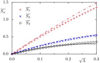
Figure 5: Average entropies $\overline{S_{\alpha}}$ for $\alpha=1,2,3$ for the coupled kicked rotors (symbols) in comparison with the perturbative results, Eq. (76), full line for $\overline{S_{3}}$ and dashed line for $\overline{S_{2}}$, and Eq. (78) for $\overline{S_{1}}$, dashed-dotted line.

IV.3 Moment at $\alpha=1/2$ and distance to the closest maximally entangled state.

The averaged moment for $\alpha=1/2$ indicates the distance of the eigenfunction to the closest maximally entangled state. In the quantum information context the “singlet fraction” HorHorHor1999 essentially measures the same quantity. It is the highest $\alpha$ value for which the moment depends on subsystem size; note the trivial case of $\alpha=0$ for which the moment is simply the subsystem dimension $N$. The case $\alpha=1/2$ is marginal and the moment is shown to grow as a logarithm of system dimensionality, whereas for $\alpha>1/2$ the moments are independent (except through the definition of $\Lambda$). This signals a breakdown of the description with a single universal dimensionless parameter, and the smaller Schmidt eigenvalues all contribute significantly to the average value of the moments.

As in the case of regularization, the divergence in Eq. (76) for $\alpha=1/2$ is indicative of a change in the functional $\Lambda$ dependency. However the largest eigenvalue moment $\overline{\lambda_{1}^{1/2}}$ given in Eq. (69), even with the $C_{3}(1/2)\Lambda$ correction is still valid. The critical quantity is the integral in Eq. (59). As the value of $\alpha$ decreases, the importance of distant levels increases. Although, the number of Schmidt eigenvalues is equal to $N$, for $\alpha>1/2$ the decay of the integrand is fast enough that in the $N\rightarrow\infty$ limit there is no difference whether the upper integration bound is finite or not. For $\alpha=1/2$ this is not true and the fact that $N$, no matter how large, has a finite value must be accounted for. A good approximation is to change the limits of integration over $s$ from $-\infty\leq s\leq\infty$ to $-(N-1)/2\leq s\leq(N-1)/2$. With the substitution $\sqrt{4\Lambda w}=s\,\tan\theta$ and using the fact that $4\sqrt{\Lambda w}/(N-1)\ll 1$, the integral in Eq. (59) leads the following modification of Eq. (68),

$$C_{2}(1/2)=2\sqrt{\pi}\int_{4\frac{\sqrt{\Lambda w}}{N-1}}^{\pi/2}\dfrac{1}{\sin^{2}\theta}\sin\frac{\theta}{2}\,d\theta.$$ (79)

The $\theta$ integral can be done exactly, and again using the fact that $N$ is large and $\Lambda$ small, the following approximation can be derived

$$\begin{split}\sum_{j>1}\overline{\sqrt{\lambda_{j}}}=\sqrt{\pi\Lambda}\,\biggl{[}&\ln\left(\frac{2(N-1)}{\sqrt{\Lambda}}\right)+\frac{\gamma}{2}+\sqrt{2}\\ &-2-\ln(1+\sqrt{2})\biggr{]}.\end{split}$$ (80)

Combining this with the result for the $\alpha=1/2$ moment of the largest eigenvalue in Eq. (69) gives the leading order term

$$\overline{\mu_{1/2}}=1+\sqrt{\pi\Lambda}\left[\ln\left(\frac{2(N-1)}{\sqrt{\Lambda}}\right)+\frac{\gamma}{2}-2\right].$$ (81)

Thus the diverging $C_{2}(\alpha)$ as $\alpha\rightarrow 1/2$ gives rise to the term proportional to $\ln(N/\sqrt{\Lambda})$. As a consequence we obtain a dependence on $N$ and as well as a different leading order $\Lambda$ dependency proportional to $-\sqrt{\Lambda}\ln(\Lambda)$, rather than $\sqrt{\Lambda}$ which is valid for moments $\alpha>1/2$.

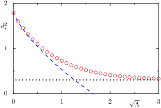
Figure 6: Square of the distance to the closest maximally entangled state $d_{*}^{2}$ (circles) as defined in Eq. (18) for the coupled kicked rotors as function of $\sqrt{\Lambda}$. The dashed line is the perturbative prediction for $\overline{d_{*}^{2}}$ using Eq. (82) and $(d_{*}^{\text{product}})^{2}=1.8$, see Eq. (19). For larger $\sqrt{\Lambda}$ an approach towards $\overline{d_{*}^{2}}_{\text{RMT}}=2(1-8/3\pi)$, see Eq. (21), (dotted line) for a typical random state takes place.

Not only is the moment $\alpha=1/2$ therefore an interesting limiting moment, but it is also of importance due to its relationship via Eq. (18) to the distance from the closest maximally entangled state. It follows from Eq. (18) and Eq. (81) that

$$\overline{d_{*}^{2}}=(d_{*}^{\text{product}})^{2}-2\sqrt{\frac{\pi\Lambda}{N}}\,\left[\ln\left(\frac{2(N-1)}{\sqrt{\Lambda}}\right)+\frac{\gamma}{2}-2\right].$$ (82)

Note that for $\Lambda=0$, the distance is that of a product state as given in Eq. (19). Figure 6 shows the transition of $\overline{d_{*}^{2}}$ going from the situation of product states at $\Lambda=0$ to typical random states at $\sqrt{\Lambda}=3$ for the coupled kicked rotors. Eq. (82) describes the initial behavior up to approximately $\sqrt{\Lambda}=0.5$ very well.

V Probability densities of Schmidt eigenvalues and entropies

Having completed the perturbation theory of the eigenvalue moments and entanglement entropies, consider the probability densities of the eigenvalues of the reduced density matrices. For $\Lambda\gg 1$, the Marčenko-Pastur law, Eq. (9), holds for the eigenvalue density of states. For $\Lambda=0$, the density is a unit $\delta$ function at unity and an $N-1$ weighted $\delta$ function at the origin. For very weak interactions, the density breaks away from the $\delta$ function form limit and is dominated by the largest and second largest eigenvalues. Note that the probability density of $\lambda_{1}$ in the strongly coupled regime is the extreme value statistics of Tracy-Widom, as it follows the same universality class of fixed trace Wishart ensembles Nec2007 .

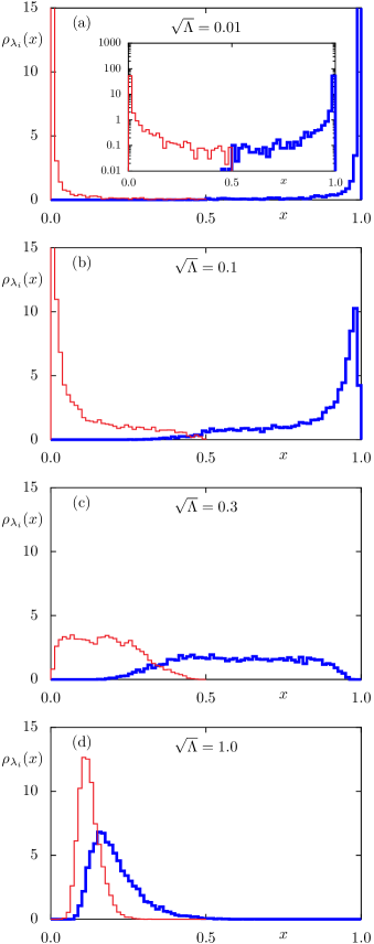
Figure 7: Probability densities $\rho_{\lambda_{1}}(x)$, thick blue histogram, and $\rho_{\lambda_{2}}(x)$, thin red histogram, for the coupled kicked rotors for $\sqrt{\Lambda}=0.01$, $0.1$, $0.3$, and $1.0$.

Figure 7 shows the probability densities $\rho_{\lambda_{1}}(x)$ and $\rho_{\lambda_{2}}(x)$. For $\Lambda\ll 1$, the density of the largest eigenvalue $\lambda_{1}$ is sharply peaked around its unperturbed value of $1$, while $\lambda_{2}$ is similarly peaked around $0$. The two densities appear almost mirror symmetric about $1/2$, and both have prominent tails extending to $1/2$, indicating instances when both of the them have large excursions away from their unperturbed values due to near degeneracies. A more detailed view of these tails is shortly developed, where power laws and stable densities exist, and the mirror symmetry is seen to be an illusion. For moderately larger couplings this picture gets modified. The probability of the largest eigenvalue develops a tail that crosses $1/2$ and the densities have an overlapping range. A curious feature that appears for $\sqrt{\Lambda}\sim 0.3$ is that the largest eigenvalue density is characterized by an almost uniform density over a wide interval. For even larger coupling the densities tend to significantly overlap and approach their random matrix extreme value statistical laws. Further results in this strong coupling regime are postponed for discussion in Sect. VI after the perturbative regime is considered in detail.

V.1 Perturbative regime

Recall that perturbatively the two largest eigenvalues $\lambda_{1}$ and $\lambda_{2}$ are fluctuating variables which from Eqs. (31) and (32), after regularization are given by

$$\begin{split}\lambda_{1}&=1-\frac{1}{2}\sum_{j}\left(1-\frac{1}{\sqrt{1+4\Lambda w_{j}/s_{j}^{2}}}\right),\,\\ \lambda_{2}&=\frac{1}{2}\left(1-\frac{1}{\sqrt{1+4\Lambda w/s^{2}}}\right).\end{split}$$ (83)

where the transition strength $w_{j}$ and $w$ is distributed according to $\rho_{w}(x)=\exp(-x)$. The spacings $s_{j}$ refer to transtions from a fixed state to all others; we will take it as independent and uniform in $[-M/2,M/2]$, where $M\gg 1$ is the number of terms in the sum for $\lambda_{1}$. This leads to a Poisson process for the ordered spacings. The spacing $s$ in $\lambda_{2}$ is the closer neighbor used in Eq. (41) and is distributed according $\rho_{\text{CN}}(s)=2\exp(-2s)$.

V.1.1 Probability density of the second largest eigenvalue

Treating $\lambda_{2}$ first, the second part of Eq. (83) and the subsequent considerations imply that its probability density is given by

$$\begin{split}&\rho_{\lambda_{2}}(x)=\\ &\int_{0}^{\infty}2e^{-2s}ds\int_{0}^{\infty}e^{-w}dw\ \delta\left[x-\frac{1}{2}\left(1-\frac{1}{\sqrt{1+4\Lambda w/s^{2}}}\right)\right]\\ &=\int_{0}^{\infty}\frac{y^{2}}{4\Lambda(1-2x)^{3}}\exp\left(-\frac{1}{4}g_{\Lambda}(x)\,y^{2}-y\right)\,dy,\end{split}$$ (84)

where the $w$ integral is performed first, $y=2s$, and

$$g_{\Lambda}(x)=\frac{x(1-x)}{\Lambda(1-2x)^{2}}.$$

The function $g_{\Lambda}(x)$, suggested by perturbation theory, is symmetric about $x=1/2$, i.e. $g_{\Lambda}(x)=g_{\Lambda}(1-x)$. It includes a scaling by $\Lambda$, which magnifies the eigenvalue $\lambda_{2}$, and the value becomes arbitrarily large whenever the second largest eigenvalue gets close to $1/2$.

This implies the remarkable result that for the variable $u_{2}=g_{\Lambda}(\lambda_{2})$ there is a universal density independent of $\Lambda$,

$$\begin{split}\rho_{u_{2}}(u)&=\frac{1}{4}\int_{0}^{\infty}e^{-t}e^{-t^{2}u/4}t^{2}dt\\ &=-\frac{1}{u^{2}}+\frac{\sqrt{\pi}}{2u^{5/2}}\left((2+u)\exp\left(1\over u\right)\text{erfc}\left(1\over\sqrt{u}\right)\right).\end{split}$$ (85)

Recall that the complementary error function is $\text{erfc}(x)=1-(2/\sqrt{\pi})\int_{0}^{x}e^{-t^{2}}dt\approx 1-2x/\sqrt{\pi}$, the approximation being valid for $x\approx 0$. Thus for $u\gg 1$, the density of $\rho_{u_{2}}(u)$ has a power-law tail $\sim\sqrt{\pi}/(2u^{3/2})$.

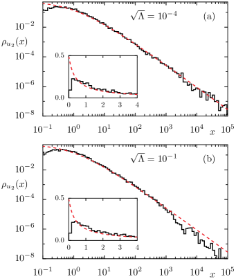
Figure 8: Probability density $\rho_{u_{2}}(x)$ for $u_{2}=g_{\Lambda}(\lambda_{2})$ in a double-logarithmic representation for the coupled kicked rotors. The dashed curves (red) shows the analytical result (85). The insets show the same densities in a linear representation.

Figure 8 illustrates the validity of the power-law tail over several orders of magnitude of $\sqrt{\Lambda}$. Although the power-law tail remains quite intact even for larger coupling strengths, such as $\sqrt{\Lambda}=0.1$, deviations are visible around $u\sim 1$ even for the smallest $\Lambda$ used. This is in the regime when $\lambda_{2}\sim\Lambda$, whereas the average $\lambda_{2}$ is much higher, being $\sim\sqrt{\Lambda}$, see Eq. (49). Thus, it appears that the current approximations used for the second eigenvalue are not good enough to capture these very small values accurately. Indeed, the average is also calculated to within $\mathcal{O}(\Lambda)$. The deviations then reflect the need for higher order perturbation theory. Note also that $\overline{u_{2}}=\infty$ due to its density having a power-law tail $u^{-3/2}$, and reflects the fact that the average of $\lambda_{2}$ is not of order $\Lambda$.

V.1.2 Density of the largest eigenvalue

The largest eigenvalue $\lambda_{1}$ is related to a sum over many terms each arising from such heavy–tailed densities and is hence naturally related to Lévy stable distributions, through the generalized central limit theorem. The first equation in Eq. (83) implies

$$1-\lambda_{1}=\sum_{j=1}^{M}x_{j},$$ (86)

where each $x_{j}$ is distributed according to the density

$$\begin{split}&\rho_{x_{j}}(x)=\\ &\frac{1}{M}\int_{-M/2}^{M/2}ds\int_{0}^{\infty}e^{-w}dw\;\delta\left[x-\frac{1}{2}\left(1-\frac{1}{\sqrt{1+4\Lambda w/s^{2}}}\right)\right]\\ &=\frac{1}{M}\int_{-M/2}^{M/2}e^{-s^{2}g_{\Lambda}(x)}\frac{s^{2}}{\Lambda(1-2x)^{3}}\,ds.\end{split}$$ (87)

Note that $s$ is uniformly distributed on $[-M/2,M/2)$ as opposed to being an exponential as in the case of the second largest eigenvalue, see Eq. (LABEL:eq:distlamb2-1).

Observe that

$$g_{\Lambda}(1-\lambda_{1})=g_{\Lambda}(\lambda_{1})\approx\sum_{j=1}^{M}y_{j},\;\;y_{j}=g(x_{j}),$$ (88)

where the approximation $g_{\Lambda}(\sum_{j}x_{j})\approx\sum_{j}g_{\Lambda}(x_{j})$ is used and justified as there is no constant term in the Taylor expansion of $g_{\Lambda}$ and the fact that to leading order $(\sum_{j>1}x_{j})^{k}\approx\sum_{j>1}x_{j}^{k}$, where the cross-terms involving independent random variables have been neglected. This is similar to the arguments that lead to the approximation in Eq. (67).

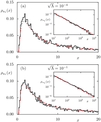
Figure 9: Probability density $\rho_{u_{1}}(x)$ of $u_{1}=g_{\Lambda}(\lambda_{1})$ for the coupled kicked rotors in comparison with the Lévy distribution (91), dashed red line. The insets show the density in a double-logarithmic representation highlighting the excellent agreement in the tails, especially for $\sqrt{\Lambda}=10^{-4}$.

The density of each $y_{j}$ is given by

$$\rho_{y_{j}}(y)=\frac{2}{M}\int_{0}^{M/2}e^{-s^{2}y}\,s^{2}\,ds\rightarrow\frac{\sqrt{\pi}}{2M}\frac{1}{y^{3/2}}.$$ (89)

If we scale $y_{j}$ to $\tilde{y}_{j}=M^{2}y_{j}/\pi$, then the density of $\tilde{y}_{j}$ has a tail that is independent of the number of terms summed and goes as $(1/2)\tilde{y}^{-3/2}$ and $g_{\Lambda}(\lambda_{1})$ is distributed as the sum

$$\frac{1}{M^{2}}\sum_{j=1}^{M}\tilde{y}_{j}.$$ (90)

Then according to a generalized central limit theorem BouGeo1990 ; UchZol1999 , the sum limits to the Lévy distribution with index $\alpha=1/2$ and scaling constant $\pi/2$. Thus if $u_{1}\equiv g_{\Lambda}(\lambda_{1})$, then it is distributed with the Lévy probability density

$$\rho_{u_{1}}(u)=\frac{\sqrt{\pi}}{2u^{3/2}}\exp\left(-\frac{\pi^{2}}{4u}\right).$$ (91)

Shown in Fig. 9 is a comparison of this density with results for the coupled kicked rotors. The power-law tail is again well reproduced and indicates the large probability with which excursions occur for the largest eigenvalue away from its unperturbed value. Therefore, if two chaotic systems are weakly coupled there is an extended regime in which the system responds very sensitively with Schmidt eigenvalues being heavy–tailed. This is reflected in the averages of the eigenvalues deviating greater from their unperturbed values than expected from a naive perturbation expansion.

V.1.3 Density of the purity

The density of the purity $\mu_{2}$ is a closely related quantity as

$$\mu_{2}=\left(1-\sum_{i>1}\lambda_{i}\right)^{2}+\sum_{i>1}\lambda_{i}^{2}\approx 1-2\sum_{i>1}\lambda_{i}(1-\lambda_{i}),$$ (92)

where cross-terms (eigenvalue correlations) have been neglected as before as they are of lower order. Using Eq. (83) we get

$$\frac{1}{2}(1-\mu_{2})=\sum_{j=1}^{N}\left(4+\dfrac{s_{j}^{2}}{\Lambda w_{j}}\right)^{-1}\equiv\sum_{j=1}^{N}x_{j},$$ (93)

with the $x_{j}$ being distributed according to

$$\rho_{x_{j}}(x)=\frac{2}{N}\int_{0}^{N/2}\exp\left(\frac{-s^{2}x}{\Lambda(1-4x)}\right)\frac{s^{2}}{\Lambda(1-4x)^{2}}ds.$$ (94)

This is therefore similar to the scenario in Eqs. (86) and (87) except that $g_{\Lambda}(x)$ is now replaced with

$$f_{\Lambda}(x)=\frac{x}{\Lambda(1-4x)}.$$ (95)

Following the same procedure as for the largest eigenvalue case gives

$$\frac{1-\mu_{2}}{2\Lambda(2\mu_{2}-1)}=\frac{S_{2}}{2\Lambda(1-2S_{2})}$$ (96)

and is Lévy distributed as in Eq. (91). The purity is written in terms of the linear entropy $S_{2}$ above which implies that the entanglement probability density, suitably scaled in the perturbative regime, is the stable Lévy distribution.

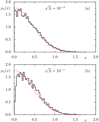
Figure 10: Probability density $\rho_{u}(x)$ of $u$ as defined in Eq. (98) based on the purity $\mu_{2}$ for the coupled kicked rotors in dependence on $\sqrt{\Lambda}$ in comparison with the half-normal density (97), red dashed line.

If $y$ is a random variable that is Lévy distributed as in Eq. (91), it is easy to see that $u=1/\sqrt{y}$ is distributed according to the “half-normal” density given by

$$\rho_{u}(x)=\sqrt{\pi}\exp(-\pi^{2}x^{2}/4)\qquad\text{with $x\geq 0$}.$$ (97)

Thus displayed in Fig. 10 for comparison with coupled kicked rotors is the probability density of the related quantity

$$u=\sqrt{\frac{2\Lambda(2\mu_{2}-1)}{1-\mu_{2}}}=\sqrt{\frac{2\Lambda(1-2S_{2})}{S_{2}}},$$ (98)

which should be distributed according to Eq. (97). Note that these expressions are expected to be valid for $\Lambda\ll 1$, where $P_{2}>1/2$. Again one observes that the agreement is very good up to $\sqrt{\Lambda}=0.01$, while for $\sqrt{\Lambda}=0.1$ clear deviations, in particular at small $u$, are visible.

V.2 Non-perturbative regime

V.2.1 Density of the purity

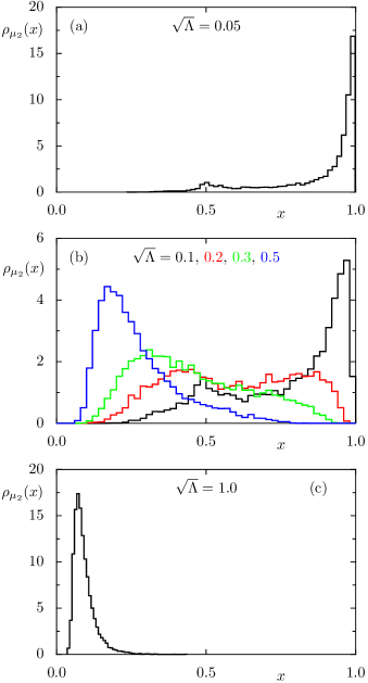
Figure 11: Probability densities $\rho_{\mu_{2}}(x)$ of the purity $\mu_{2}$ for the coupled kicked rotors for $\sqrt{\Lambda}=0.05,0.1,0.2,0.3,0.5,1.0$.

Shown in Fig. 11 is the density $\rho_{\mu_{2}}(x)$ of the purity itself, across a wide range of the transition parameter $\Lambda$. It is seen that at around $\sqrt{\Lambda}=0.1$ a prominent secondary peak appears around purity $x=1/2$. This corresponds well with the value of the interaction for which the density of the largest eigenvalue starts to overlap with that of the second largest in a significant manner as seen earlier in Fig. 7. For larger values of $\Lambda$, the other eigenvalues also compete as is illustrated in Fig. 3 and decreases the secondary peak’s purity further. The densities become unimodal once again and proceed towards to the random matrix densities with a mean value around $2/N$. Although the entire transition remains to be captured, the next section shows how the mean value and similar mean values for other entropies can be motivated to evolve in an essentially simple manner.

V.2.2 Transition of the density of Schmidt eigenvalues

For the case of strong interaction, i.e. large $\Lambda$, one expects that the statistics of any quantity of interest follows the corresponding random matrix results. The approach to this limit can be, as illustrated here, quite distinct. First, consider the density of

$$\tilde{\lambda_{i}}=N\lambda_{i},$$ (99)

which for $\Lambda$ large enough must follow the Marčenko-Pastur distribution, Eq. (9). Toward this end, consider the density of the rescaled eigenvalues. Figure 12 shows the combined density obtained from $N$ Schmidt eigenvalues for each of the $N^{2}$ eigenstates for the coupled kicked rotors. For $\sqrt{\Lambda}=3$, deviations are still clearly visible in the tail of the density visible in the inset. For $\sqrt{\Lambda}=10$ the agreement with the Marčenko-Pastur distribution is quite good apart for a small deviation in the tail, whereas for $\sqrt{\Lambda}=15$ (not shown) the agreement is excellent.

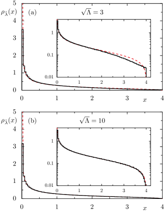
Figure 12: Density $\rho_{\tilde{\lambda}}(x)$ of all Schmidt eigenvalues, rescaled according to Eq. (99), for the coupled kicked rotors (black histogram) in comparison with the Marčenko-Pastur distribution (9) for $Q=1$, red dashed line. The inset shows the same data in the semi-logarithmic representation.

Of particular importance is the probability density of the largest eigenvalue $\lambda_{1}$, which has already been considered in the perturbative regime, see Fig. 7. In the random matrix theory limit the behavior in the tail of the Marčenko-Pastur distribution is governed by $\lambda_{1}$. In this limit a Tracy-Widom distribution $F_{2}$ is expected for the unitary case TraWid1996 ; EdeRao2005 , if one considers the appropriately rescaled variable

$$\lambda_{\text{max}}=\frac{\lambda_{1}-4/N}{2^{4/3}N^{-5/3}},$$ (100)

see e.g. (Nec2007, , Eq. (55)). Of interest is how the Tracy-Widom distribution is approached as the interaction is increased $\sqrt{\Lambda}$. Figure 13 shows that the approach is much slower than for any other statistical quantity considered in this paper: only for about $\sqrt{\Lambda}=14$ good agreement with the Tracy-Widom distribution is observed when $N=100$. Interestingly, we find that for $N=50$ already for $\sqrt{\Lambda}=6$ quite good agreement with the Tracy-Widom distribution is obtained (not shown). This gives a hint that for this statistics the transition parameter does not provide the right scaling; understanding this in detail is left for future investigation.

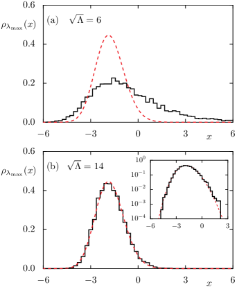
Figure 13: Density $\rho_{\lambda_{\text{max}}}(x)$ of the largest Schmidt eigenvalue $\lambda_{1}$, rescaled according to Eq. (100), for the coupled kicked rotors for different $\sqrt{\Lambda}$. For comparison the Tracy-Widom distribution, expected in the random matrix theory limit, is shown (dashed red line).

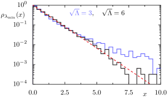
Figure 14: Density $\rho_{\lambda_{\text{min}}}(x)$ of the smallest Schmidt eigenvalue $\lambda_{N}$, rescaled according to Eq. (101), for the coupled kicked rotors for $\sqrt{\Lambda}=3$ (blue) and $\sqrt{\Lambda}=6$ (black). For comparison the exponential density, expected in the random matrix limit, is shown (dashed red line).

For random matrix theory, the density of the smallest Schmidt eigenvalue $\lambda_{N}$ is proven to be exponential MajBohLak2008 using the rescaling

$$\lambda_{\text{min}}\equiv N(N^{2}-1)\lambda_{N}.$$ (101)

Figure 14 shows that for $\sqrt{\Lambda}=3$ the tail of the density is clearly not following the exponential behavior, but $\sqrt{\Lambda}=6$ shows good agreement.

VI Recursively embedded perturbation theory

The analytical expressions obtained thus far are perturbative, i.e. $\Lambda\ll 1$, but random matrix theory is expected to reproduce the entire transition for chaotic systems. The opposite limit, $\Lambda\rightarrow\infty$, is also likely to allow for analytic calculations. As the main object of interest has been the spectra of the reduced density matrices, the relevant random matrix ensemble is the fixed-trace Wishart ensemble ZycSom2001 for which a variety of results are already known ZycSom2001 ; SomZyc2004 ; KumSamAna2017 ; MajBohLak2008 ; MajVer2009 ; NadMajVer2011 . Thus it would be interesting to connect the perturbative regimes with various power laws to this random matrix regime. Here, we restrict to the average of moments rather than their probability densities.

Increasing $\Lambda$ gradually from $0$, the eigenvalues of the reduced density matrix of an eigenstate of the full system get added one at a time, see Fig. 3 for an illustration in terms of the averages $\overline{\lambda_{i}}$. Therefore this defines successive regimes in which one Schmidt eigenvalue after another starts to increase significantly away from 0. In the first regime there are roughly $\sim\sqrt{\Lambda}N^{2}$ eigenstates whose reduced density matrix has two prominent eigenvalues. Thus for $\sqrt{\Lambda}\ll 1/N^{2}$ the largest eigenvalue is still nearly unity for all eigenstates. For $\sqrt{\Lambda}\sim 1/N^{2}$ due to near degeneracies in the system’s spectrum, certain eigenstate pairs suddenly appear in uncorrelated, widely separated parts of the spectrum that have two dominant eigenvalues $\lambda_{1}$ and $\lambda_{2}$. They are responsible for the averages that deviate by an order $\sqrt{\Lambda}$ (as opposed to $\mathcal{O}(\Lambda)$) from their values in the absence of interactions. As $\Lambda$ is continuously increased, clusters of three levels, whose eigenstates have three significant eigenvalues appear, the third one being of the order of $\Lambda\ln\Lambda$ in the previous regime of pairs only. In this regime, the third Schmidt eigenvalue starts to develop significance and there is a regime where the fourth is also important and so on.

This scenario suggests an analysis that can capture the essence of the successive regimes in the transition. Consider the first regime and let the pair of unperturbed states $|kl\rangle$ and $|k_{1}l_{1}\rangle$ be one such doublet creating a pair of eigenstates, one of whom’s Schmidt decomposition is very nearly

$$\sqrt{\nu_{1}}\,|kl\rangle+\sqrt{\nu_{1}^{\prime}}\,|k_{1}l_{1}\rangle,$$ (102)

where $\nu_{1}+\nu_{1}^{\prime}=1$. For the other member of the pair, $\nu_{1},\,\nu_{1}^{\prime}$ are interchanged, so assume that $\nu_{1}^{\prime}\leq\nu_{1}$. Further increase in the interaction starts to mix in say $|k_{2}l_{2}\rangle$, such that the Schmidt decomposition is now approximately

$$\sqrt{\nu_{2}}\left(\sqrt{\nu_{1}}\,|kl\rangle+\sqrt{\nu_{1}^{\prime}}\,|k_{1}l_{1}\rangle\right)+\sqrt{\nu_{2}^{\prime}}|k_{2}l_{2}\rangle,$$ (103)

again with $\nu_{2}+\nu_{2}^{\prime}=1$ and $\nu_{2}^{\prime}\leq\nu_{2}$. At this stage there are three prominent Schmidt eigenvalues and the corresponding probabilities: $\nu_{2}\nu_{1},\nu_{2}\nu_{1}^{\prime},\nu_{2}^{\prime}$. The process is now iterated, thus schematically corresponds to a fragmentation process of the interval $[0,1]$ into smaller pieces that add to $1$:

$$\begin{split}\{\nu_{1},\nu_{1}^{\prime}\}&\rightarrow\{\nu_{2}\nu_{1},\nu_{2}\nu_{1}^{\prime},\nu_{2}^{\prime}\}\\ &\rightarrow\{\nu_{3}\nu_{2}\nu_{1},\nu_{3}\nu_{2}\nu_{1}^{\prime},\nu_{3}\nu_{2}^{\prime},\nu_{3}^{\prime}\}\rightarrow\cdots,\end{split}$$ (104)

where $\nu_{j}^{\prime}+\nu_{j}=1$ at all stages, but $\nu_{j}$ is a random variable. At a particular generation let the fractions be $\{\lambda_{1},\cdots,\lambda_{K-1}\}$ and the associated moment be $\mu_{\alpha}=\sum_{j=1}^{K-1}\lambda_{j}^{\alpha}$. Then after the next level

$$\mu^{\prime}_{\alpha}=\nu_{K}^{\alpha}\mu_{\alpha}+(\nu_{K}^{\prime})^{\alpha}.$$ (105)

Thus

$$\mu^{\prime}_{\alpha}-\mu_{\alpha}=-(1-\nu_{K}^{\alpha}-(\nu_{K}^{\prime})^{\alpha})\,\mu_{\alpha}+(\nu_{K}^{\prime})^{\alpha}(1-\mu_{\alpha}).$$ (106)

Now consider only the leading order of $\overline{\mu_{\alpha}}$ in Eq. (74) and assume that $\nu_{K}$ and $\nu_{K}^{\prime}$ have the same properties as $\lambda_{1}$ and $\lambda_{2}$, in particular that their moments satisfy Eq. (59) and Eq. (67). Note that Eq. (59) is also the moment of $\lambda_{2}$ as the other eigenvalues contribute at a smaller order of $\sqrt{\Lambda}$. Putting these together we get an equation for the averages,

$$\overline{\mu_{\alpha}^{\prime}}-\overline{\mu_{\alpha}}=-C(\alpha)\sqrt{\Lambda}\ \overline{\mu_{\alpha}}+{\mathcal{O}}(\Lambda),$$ (107)

which suggests that the fragmentation process occurs at a rate proportional to $\sqrt{\Lambda}$. Taking into account the known behavior of $\overline{\mu_{\alpha}}$ around $\sqrt{\Lambda}=0$ leads to the differential equation

$$\frac{\partial\overline{\mu_{\alpha}}}{\partial\sqrt{\Lambda}}=-C(\alpha)\overline{\mu_{\alpha}}.$$ (108)

This recursively embedded perturbative argument suggests a simple exponential extension of the perturbation expansions. That is the differential equation solution

$$\overline{\mu_{\alpha}}\approx\exp\left(-C(\alpha)\sqrt{\Lambda}\right),$$ (109)

is expected to be valid for larger $\Lambda$ than does the linear perturbative result in Eq. (74). This supports an exponential decay of moments, in particular the purity ($\alpha=2$), as the interaction is increased.

In the $\Lambda\rightarrow\infty$ limit, the known random matrix asymptotic (large $N$) result is

$$\overline{\mu_{\alpha}^{\infty}}=\mathcal{C}_{\alpha}/N^{\alpha-1},$$ (110)

where the $\mathcal{C}_{\alpha}$ are Catalan numbers (DLMF, , §26.5.), defined usually for integer value of $\alpha$. The $\overline{\mu_{\alpha}^{\infty}}$, being the moments of the Marčenko-Pastur distribution (9) are well-defined for all $\alpha\geq 0$ and hence $\mathcal{C}_{\alpha}$ are well-defined as well.

A simple interpolation between the exponential decay of the moments and their random matrix value is given by

$$\overline{\mu_{\alpha}}\approx\exp\left(-\frac{C(\alpha)}{1-\overline{\mu^{\infty}_{\alpha}}}\sqrt{\Lambda}\right)\left(1-\overline{\mu^{\infty}_{\alpha}}\right)+\overline{\mu^{\infty}_{\alpha}}.$$ (111)

The arguments of the exponentials in Eq. (109) get modified by the asymptotic values so that the small $\Lambda$ perturbative result is unchanged, yet the asymptotic value is reached. Using (8) this gives the for the entropies

$$\overline{S_{\alpha}(\Lambda)}\approx\left[1-\exp\left(-\frac{C(\alpha)}{(\alpha-1)\overline{S_{\alpha}^{\infty}}}\sqrt{\Lambda}\right)\right]\overline{S^{\infty}_{\alpha}},$$ (112)

where

$$\overline{S_{\alpha}^{\infty}}=\frac{1-\mathcal{C}_{\alpha}N^{1-\alpha}}{\alpha-1}.$$ (113)

The asymptotic entropies $\overline{S_{\alpha}^{\infty}}$ are reached at the end of the transition, and although Eq. (113) is valid for $\alpha>1$, it is known that $\overline{S_{1}^{\infty}}=\ln N-\frac{1}{2}$. For $\alpha=1$ one has the important case of the von Neumann entropy, which, however, has to be treated separately. Its increase is governed by the limit of $C(\alpha)/(\alpha-1)$ as $\alpha\rightarrow 1$ which is equal to $\pi^{3/2}$, consistent with Eq. (78). Explicitly the von Neumann entropy is

$$\overline{S_{1}(\Lambda)}\approx\left[1-\exp\left(-\frac{\pi^{3/2}}{\overline{S_{1}^{\infty}}}\sqrt{\Lambda}\right)\right]\overline{S^{\infty}_{1}}.$$ (114)

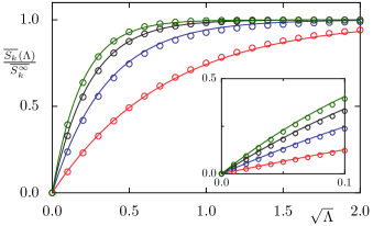
Figure 15: The average eigenstate entropies $\overline{S_{\alpha}}$ for von Neumann ($S_{1}$), and $\alpha=2,3,4$ as a function of $\sqrt{\Lambda}$. The lowest curve is for von Neumann, and the approach to asymptotic values is faster for larger $\alpha$ values. The circles are for the coupled kicked rotors. The lines correspond to Eq. (112). The inset is a magnification of the small-$\Lambda$ region.

Figure 15 shows the von Neumann entropy and $S_{2},S_{3},S_{4}$ for the coupled kicked rotors. The agreement is surprisingly good with Eqs. (112) and (114). The inset may be compared with Fig. 5, where deviations are visible from the perturbation theory at values of $\sqrt{\Lambda}$ that is one order of magnitude smaller. Overall the exponential continuation along with the random matrix value seems to give the full transition from uncoupled, unentangled states to generic states with nearly maximal entanglement entropy.

VII Summary and outlook

The results obtained in this paper apply to a rather general class of weakly interacting bipartite systems. The basic assumption is that each of the subsystems can be considered quantum chaotic in the sense that it can be described by random matrix statistics for the eigenvalues and eigenvectors. The random matrix ensemble, Eq. (23), describes the universal transition from the statistics of non-interacting systems to those of a fully interacting case, as long as it is characterized as a function of the unitless transition parameter $\Lambda$, Eq. (35). This transition is described by a generalized universality class of a dynamical symmetry breaking nature. While the subsystems are assumed to follow random matrix statistics, the interaction between the subsystems is kept general. Thus, this approach, numerically illustrated for the example of the coupled kicked rotors, applies equally well to few- and many-body systems, e.g. interacting particles in quantum dots, spin chains, coupled quantum maps, and Floquet systems. Many dynamical symmetry breaking scenarios may be imagined for many-body systems, e.g., spin-spin interactions or weak environmental coupling.

A random matrix transition ensemble is used to derive the entanglement properties of two interacting subsystems. Based on a perturbative treatment, the single universal transition parameter $\Lambda$ is determined in terms of the interaction. Starting from the non-interacting case, $\Lambda=0$, the entanglement between the subsystems increases to being nearly maximal, i.e. to that of random states in the full Hilbert space. Quantitatively the entanglement may be characterized by the purity, HCT entropies, and the von Neumann entropy. All these can be computed using the Schmidt eigenvalues $\lambda_{i}$ of the reduced density matrix. Based on perturbation theory explicit expressions for the largest and second largest eigenvalue of the reduced matrix are obtained. Using an appropriate regularization, predictions for the averages $\overline{\lambda_{1}}$ and $\overline{\lambda_{2}}$ are derived, which are valid for small values of $\sqrt{\Lambda}$. In this regime good agreement with numerical results for the coupled kicked rotors is found. Furthermore, the average moments $\sum_{j>1}\overline{\lambda_{j}^{\alpha}}$ and $\overline{\lambda_{1}^{\alpha}}$ are obtained perturbatively up to order $\mathcal{O}(\Lambda)$. Based on these moments, a perturbative prediction for the entanglement entropies, Eq. (7), is obtained. A comparison with numerical results for the coupled kicked rotors shows that the perturbative results provide a good approximation up to about $\sqrt{\Lambda}=0.3$. This indicates that the theoretical results are robust, in the sense that deviations from ideal behavior, such as discussed in App. C do not harm the agreement. A particularly interesting moment is $\overline{\mu_{1/2}}$ as this indicates the distance of the eigenfunction to the closest maximally entangled state. Here the perturbative result gives good agreement with numerics up to $\sqrt{\Lambda}=0.6$.

Going beyond the average behavior of the eigenvalue moments and entanglement entropies the probability densities of the eigenvalues of the reduced density matrices are studied. The probability densities of $\lambda_{1}$ and $\lambda_{2}$, in dependence on the transition parameter $\Lambda$, show substantial tails. In the perturbative regime, a suitable rescaling of $\lambda_{2}$ has a universal density which is independent of $\Lambda$, and shows a power-law tail, found over several orders of magnitude. For the density of a rescaled $\lambda_{1}$, which is a sum of heavy-tailed densities, a generalized central limit theorem implies the Lévy distribution, which also shows a power-law tail. Closely related is the density of the linear entropy $S_{2}$, which also follows the Lévy distribution. In turn the purity $\mu_{2}=1-S_{2}$, again rescaled, shows a half normal density, which is also well seen in the numerical results for the coupled kicked rotors with good agreement at small $\sqrt{\Lambda}$ and deviations showing up for $\sqrt{\Lambda}=10^{-1}$.

In the non-perturbative regime the density of the purity shows a transition from a small amount of entanglement, $\mu_{2}$ near 1, to large entanglement, $\mu_{2}$ around $2/N$. The density of rescaled Schmidt eigenvalues approaches the Marčenko-Pastur distribution. Of particular interest is the density of the largest eigenvalue $\lambda_{1}$, which in the limit of large interaction follows the Tracy-Widom distribution. Interestingly, the approach to this limit is much slower than for any of the other statistical quantities considered in this paper, with good agreement with numerics only found for $\sqrt{\Lambda}=14$. In contrast, the approach of the density of the smallest Schmidt eigenvalue to the exponential density of the random matrix theory limit appears to be faster.

To obtain a description of the behavior of the entanglement entropies for the whole transition, a recursively embedded perturbation theory is invoked. This leads to a remarkably simple expression, Eq. (111), which actually captures the essence of the entire transition. It is found to be in very good agreement with the numerical results for the coupled kicked rotors, see Fig. 15.

Moreover, eigenstate localization as measured by the inverse participation ratio is connected to the linear entropy after subsystem averaging, as was shown in LakSriKetBaeTom2016 . Thus using a spectral averaging, this can be used as sensitive detector of non-ergodic behaviors. An interesting future direction concerns the relation between entropies and eigenvector moments.

It is interesting, that the rate of growth of entropy $S_{\alpha}$ as a function of the transition parameter, has precisely the same form as the $\alpha^{\text{th}}$ multifractal exponent of eigenstates of critical random matrix ensembles describing the physics of Anderson transitions MirEve2000 ; EveMir2008 . For example compare the leading order term in Eq. (76) with Eq. (3.20) of EveMir2008 . This is no coincidence as both are derived as a consequence of a degenerate perturbation theory that starts from Poissonian spectra. However, beyond this similarity, although there are power-laws in the systems we are investigating, if there is criticality in some sense remains to be seen. The kinds of random matrix ensembles used in this context thus far are single-particle ones  EveMir2008 ; BogGir2011a ; BogGir2011 and it is interesting to see if criticality can arise as a consequence of coupling chaotic systems.

An important future application of the results for the random matrix transition ensemble is that this provides a means to detect non-universal behaviors in terms of deviations from the obtained universal results. For example for the situation in which one or both of the subsystems shows a mixed phase space or some kind of localization of eigenstates, the results given here represent an important limit to compare with. It is reasonable to expect that at any given interaction strength the entropies derived herein are an upper bound in typical systems such as in the coupled kicked rotors.

The application of the results in the context of weakly interacting many-body system, such as spin-chains, will be of particular interest. This work raises the question how to determine the transition parameter $\Lambda$ in such situations and then investigate the universality of statistics in dependence on $\Lambda$. Besides investigating the properties of spectra and eigenfunctions, also the time-evolution of wave-packets is expected to follow a universal behavior in dependence on the transition parameter. This should also pave the way for experimental studies, e.g. using cold-atom experiments. Such results will be of importance for dynamical systems, quantum information, and condensed matter theory.

Appendix A Perturbation theory with unitary matrices

Here we derive the perturbation theory results for eigenvalues and eigenfunctions of unitary matrices. The eigenvalue results of this appendix can be found in the book by Peres Per2002 . Consider a unitary operator of the form

$$\begin{split}{\cal U}(\epsilon)&=(U_{A}\otimes U_{B})\,U_{AB}(\epsilon)\\ U_{AB}(\epsilon)&=\exp(i\epsilon V),\end{split}$$ (115)

where ${\cal H}_{A},{\cal H}_{B}$ (dimensions $N_{A}\leq N_{B}$, respectively) are assumed to be symmetry reduced subspaces, and hence there are no systematic degeneracies. It has unperturbed eigenstates separately for the individual subspaces of the direct product space given by,

$$U_{A}|j^{A}\rangle=e^{i\theta^{A}_{j}}|j^{A}\rangle\qquad U_{B}|k^{B}\rangle=e^{i\theta^{B}_{k}}|k^{B}\rangle$$ (116)

and therefore

$$(U_{A}\otimes U_{B})|j^{A}\rangle|k^{B}\rangle=e^{i\theta_{jk}}|j^{A}\rangle|k^{B}\rangle\qquad\theta_{jk}=\theta^{A}_{j}+\theta^{B}_{k}$$ (117)

The eigenstates of the full system can be denoted by a double index label $jk$. Then

$$(U_{A}\otimes U_{B})\,U_{AB}(\epsilon)|\Phi_{jk}\rangle=e^{i\varphi_{jk}}|\Phi_{jk}\rangle$$ (118)

where in the $\epsilon\rightarrow 0$ limit, $|\Phi_{jk}\rangle\rightarrow|j^{A}\rangle|k^{B}\rangle\ (=|jk\rangle)$ and $\varphi_{jk}\rightarrow\theta_{jk}$. The standard perturbation approach is to insist that $\langle jk|\Phi_{jk}\rangle=1$, thereby implying that $\langle\Phi_{jk}|\Phi_{jk}\rangle>1$, and it is necessary to renormalize the eigenvectors in a second step. The ansatzes for the unnormalized eigenvector and eigenangle are

$$\begin{split}|\Phi_{jk}\rangle&=|jk\rangle+\sum_{n=1}^{\infty}\epsilon^{n}|\Phi_{jk}^{(n)}\rangle\\ \varphi_{jk}&=\sum_{n=0}^{\infty}\epsilon^{n}\varphi_{jk}^{(n)},\end{split}$$ (119)

where it remains to calculate the $n^{th}$-order corrections $|\Phi_{jk}^{(n)}\rangle$, and the eigenangle, $\varphi_{jk}^{(n)}$. The equations to all orders can be generated by projecting a complete set of states using the unperturbed basis onto Eq. (118),

$$\begin{split}&\sum_{j^{\prime}k^{\prime}=1}^{N_{A}N_{B}}|j^{\prime}k^{\prime}\rangle\langle j^{\prime}k^{\prime}|(U_{A}\otimes U_{B})\,U_{AB}(\epsilon)|\Phi_{jk}\rangle=\\ &e^{i\varphi_{jk}}\sum_{j^{\prime}k^{\prime}=1}^{N_{A}N_{B}}|j^{\prime}k^{\prime}\rangle\langle j^{\prime}k^{\prime}|\Phi_{jk}\rangle=\\ &e^{i\theta_{j^{\prime}k^{\prime}}}\sum_{j^{\prime}k^{\prime}=1}^{N_{A}N_{B}}|j^{\prime}k^{\prime}\rangle\langle j^{\prime}k^{\prime}|U_{AB}(\epsilon)|\Phi_{jk}\rangle\ ,\end{split}$$ (120)

then substituting the anzatses of Eq. (119), the exponential form of the interaction in Eq. (115), and creating a hierarchy of equations by collecting terms of equal order in $\epsilon$. Each equation must hold individually for any particular term in the summation $jk^{\prime}$ above. The first equation is,

$$\begin{split}&e^{i\theta_{jk}}\left[i\delta_{jk,j^{\prime}k^{\prime}}\varphi^{(1)}_{jk}+\left(1-\delta_{jk,j^{\prime}k^{\prime}}\right)\langle j^{\prime}k^{\prime}|\Phi_{jk}^{(1)}\rangle\right]\\ &=e^{i\theta_{{j^{\prime}k}^{\prime}}}\left[\left(1-\delta_{jk,j^{\prime}k^{\prime}}\right)\langle j^{\prime}k^{\prime}|\Phi_{jk}^{(1)}\rangle+i\langle j^{\prime}k^{\prime}|V|jk\rangle\right]\end{split}$$ (121)

The $jk=j^{\prime}k^{\prime}$ term gives the expected relation

$$\varphi^{1}_{jk}=\langle jk|V|jk\rangle$$ (122)

and the $jk\neq j^{\prime}k^{\prime}$ terms give

$$\langle j^{\prime}k^{\prime}|\Phi_{jk}^{(1)}\rangle=\frac{i\langle j^{\prime}k^{\prime}|V|jk\rangle}{e^{i\left(\theta_{jk}-\theta_{j^{\prime}k^{\prime}}\right)}-1}.$$ (123)

In the limit of $N_{A}\rightarrow\infty$, only differentially small angle differences are perturbative and this equation reduces to the familiar form arising with perturbation theory of Hamiltonian systems,

$$\langle j^{\prime}k^{\prime}|\Phi_{jk}^{(1)}\rangle=\frac{\langle j^{\prime}k^{\prime}|V|jk\rangle}{\theta_{jk}-\theta_{j^{\prime}k^{\prime}}},$$ (124)

where the eigenangles appear instead of the eigenenergies.

The equation for the second order corrections is longer and it is simpler to isolate the $\delta_{jk,j^{\prime}k^{\prime}}$ terms from those with $1-\delta_{jk,j^{\prime}k^{\prime}}$. First, the $\delta_{jk,j^{\prime}k^{\prime}}$ terms lead to

$$i\varphi_{jk}^{(2)}-\frac{(\varphi_{jk}^{(1)})^{2}}{2}=i\langle jk|V|\Phi_{jk}^{(1)}\rangle-\frac{1}{2}\langle jk|V^{2}|jk\rangle.$$ (125)

Substituting in the solutions from the first order equations gives

$$\varphi_{jk}^{(2)}=\sum_{j^{\prime}k^{\prime}\neq jk}^{N_{A}N_{B}}\left[\frac{i}{e^{i\left(\theta_{jk}-\theta_{j^{\prime}k^{\prime}}\right)}-1}+\frac{i}{2}\right]\left|\langle j^{\prime}k^{\prime}|V|jk\rangle\right|^{2}.$$ (126)

Perhaps it is less than immediately obvious that the second order eigenangle correction is real, but consider that

$$\begin{split}\frac{i}{e^{i\left(\theta_{jk}-\theta_{j^{\prime}k^{\prime}}\right)}-1}+\frac{i}{2}&=\frac{\sin\left(\theta_{jk}-\theta_{j^{\prime}k^{\prime}}\right)}{4\sin^{2}\left(\frac{\theta_{jk}-\theta_{j^{\prime}k^{\prime}}}{2}\right)}\\ &=\frac{1}{2}\cot\left(\frac{\theta_{jk}-\theta_{j^{\prime}k^{\prime}}}{2}\right)\end{split}$$ (127)

and also in the $N_{A}\rightarrow\infty$ limit, the usual form of the second order eigenvalue correction is recovered

$$\varphi_{jk}^{(2)}=\sum_{j^{\prime}k^{\prime}\neq jk}^{N_{A}N_{B}}\frac{\left|\langle j^{\prime}k^{\prime}|V|jk\rangle\right|^{2}}{\theta_{jk}-\theta_{j^{\prime}k^{\prime}}}.$$ (128)

That leaves the equation resulting from the second order terms without the $j^{\prime}k^{\prime}=jk$ terms. After a bit of algebra and grouping terms, this gives

$$\begin{split}&\langle j^{\prime}k^{\prime}|\Phi_{jk}^{(2)}\rangle=\frac{i}{e^{i\left(\theta_{jk}-\theta_{j^{\prime}k^{\prime}}\right)}-1}\times\\ &\left[\sum_{j^{\prime\prime}k^{\prime\prime}\neq jk}^{N_{A}N_{B}}\frac{\langle j^{\prime}k^{\prime}|V|j^{\prime\prime}k^{\prime\prime}\rangle\langle j^{\prime\prime}k^{\prime\prime}|V|jk\rangle\sin\left(\theta_{jk}-\theta_{j^{\prime\prime}k^{\prime\prime}}\right)}{4\sin^{2}\left(\frac{\theta_{jk}-\theta_{j^{\prime\prime}k^{\prime\prime}}}{2}\right)}+\right.\\ &\qquad\qquad\left.\frac{\langle j^{\prime}k^{\prime}|V|jk\rangle\langle jk|V|jk\rangle\sin\left(\theta_{jk}-\theta_{j^{\prime}k^{\prime}}\right)}{4\sin^{2}\left(\frac{\theta_{jk}-\theta_{j^{\prime}k^{\prime}}}{2}\right)}\right],\end{split}$$ (129)

which also reduces to the expected expressions in the $N_{A}\rightarrow\infty$ limit. Renormalizing the eigenfunction alters the unit coefficient in front of $|jk\rangle$ in the expansion to

$$|\Phi_{jk}\rangle=\left[1-\frac{\epsilon^{2}}{8}\sum_{j^{\prime}k^{\prime}\neq jk}^{N_{A}N_{B}}\frac{\left|\langle j^{\prime}k^{\prime}|V|jk\rangle\right|^{2}}{\sin^{2}\left(\frac{\theta_{jk}-\theta_{j^{\prime}k^{\prime}}}{2}\right)}\right]|jk\rangle+...$$ (130)

also with the expected $N_{A}\rightarrow\infty$ limit.

Appendix B Transition parameter

In this appendix we derive expression (42) for the transition parameter $\Lambda$. Consider the bipartite unitary operator in Eq. (2) for which we want to calculate $v^{2}$, the mean square off-diagonal matrix element of $U_{AB}(\epsilon)$ in the basis in which $U_{A}$ and $U_{B}$ are diagonal. To simplify notation we omit the dependence on $\epsilon$. Moreover, for convenience we assume that $U_{A,B}$ are sampled independently from the CUE (of $N_{A}\times N_{A}$, and $N_{B}\times N_{B}$ unitary matrices respectively) and averaging is also performed over this ensemble.

In the unperturbed basis, denote the off-diagonal matrix element

$$z_{kl;k^{\prime}l^{\prime}}=\sum_{m=1}^{N_{A}}\sum_{n=1}^{N_{B}}u_{km}u_{k^{\prime}m}^{*}w_{ln}w_{l^{\prime}n}^{*}(U_{AB})_{mn},$$

where $(k,l)\neq(k^{\prime},l^{\prime})$, and $(U_{AB})_{mn}=\langle mn|U_{AB}|mn\rangle$ is a diagonal matrix element due to the interaction and $u,w$ are two independent $N_{A},N_{B}$–dimensional unitary matrices, respectively, which diagonalize the unperturbed part. The averaging is done over the Haar measure on unitary matrices. Using the independence of $u$ and $w$, and the relation

$$\overline{u_{km}u_{k^{\prime}m^{\prime}}u^{*}_{k^{\prime}m}u^{*}_{km^{\prime}}}=\frac{\delta_{mm^{\prime}-1/N_{a}}}{N_{A}^{2}-1},$$

gives

$$\begin{split}~{}&v^{2}=\overline{|z_{kl;k^{\prime}l^{\prime}}|^{2}}\\ ~{}&=\frac{\sum_{m,m^{\prime}}^{N_{A}}\sum_{n,n^{\prime}}^{N_{B}}\left[\delta_{mm^{\prime}}\delta_{nn^{\prime}}-\frac{\delta_{nn^{\prime}}}{N_{A}}-\frac{\delta_{mm^{\prime}}}{N_{B}}+\frac{1}{N_{A}N_{B}}\right]}{(N_{A}^{2}-1)(N_{B}^{2}-1)}\\ &~{}\quad\times(U_{AB})_{mn}(U_{AB})^{*}_{m^{\prime}n^{\prime}}.\end{split}$$ (131)

This series can be rewritten as

$$\begin{split}&v^{2}=\dfrac{N_{A}^{2}N_{B}^{2}}{(N_{A}^{2}-1)(N_{B}^{2}-1)}\times\\ &\left(1+\left|\frac{\text{tr}U_{AB}}{N_{A}N_{B}}\right|^{2}-\frac{1}{N_{A}}\,\left\|\frac{U^{(A)}}{N_{B}}\right\|^{2}-\frac{1}{N_{B}}\,\left\|\frac{U^{(B)}}{N_{A}}\right\|^{2}\right),\end{split}$$ (132)

where $U^{(A)}=\text{tr}_{B}U_{AB}$, $U^{(B)}=\text{tr}_{A}U_{AB}$, and $\|X\|=\text{tr}(XX^{\dagger})$ is Hilbert-Schmidt norm.

The transition parameter $\Lambda=v^{2}/D^{2}$, where $D=\frac{2\pi}{N_{A}N_{B}}$ is the mean level spacing, then takes the form

$$\begin{split}&\Lambda=\dfrac{N_{A}^{3}N_{B}^{3}}{4\pi^{2}(N_{A}^{2}-1)(N_{B}^{2}-1)}\times\\ &\left(1+\left|\frac{\text{tr}U_{AB}}{N_{A}N_{B}}\right|^{2}-\frac{1}{N_{A}}\,\left\|\frac{U^{(A)}}{N_{B}}\right\|^{2}-\frac{1}{N_{B}}\,\left\|\frac{U^{(B)}}{N_{A}}\right\|^{2}\right).\end{split}$$ (133)

Next we evaluate $\Lambda$ explicitly for the model in Eq. (2) by performing the averaging over $\xi_{j}$. For this we treat every term in the sum in Eq. (133) separately,

$$\overline{\left|\frac{\text{tr}U_{AB}}{N_{A}N_{B}}\right|^{2}} =\frac{1}{N_{A}^{2}N_{B}^{2}}\overline{\sum_{j,j^{\prime}=1}^{N_{A}N_{B}}e^{2\pi i\epsilon\xi_{j}}e^{-2\pi i\epsilon\xi_{j^{\prime}}}}$$

$$=\frac{1}{N_{A}^{2}N_{B}^{2}}\left[\sum_{j=1}^{N_{A}N_{B}}1+\sum_{j\neq j}\overline{e^{2\pi i\epsilon(\xi_{j}-\xi_{j^{\prime}})}}\right].$$

As the $\xi_{j}$’s are independent uniform random variables in $[-1/2,1/2)$, their difference $z=\xi_{j}-\xi_{j^{\prime}}$ has the probability density function,

$$\rho_{z}(x)=\begin{cases}1+x&\text{ for }-1<x<0\\ 1-x&\text{ for }0\leq x<1\\ 0&\text{ otherwise}.\end{cases}$$ (134)

Using $\int_{-1}^{1}e^{2\pi i\epsilon x}\rho_{z}(x)dx=\frac{\sin^{2}(\pi\epsilon)}{\pi^{2}\epsilon^{2}}$ gives

$$\overline{\left|\frac{\text{tr}U_{AB}}{N_{A}N_{B}}\right|^{2}}=\frac{1}{N_{A}N_{B}}+\left(1-\frac{1}{N_{A}N_{B}}\right)\frac{\sin^{2}(\pi\epsilon)}{\pi^{2}\epsilon^{2}}.$$

Similarly,

$$\overline{\frac{1}{N_{A}}\,\left\|\frac{U^{(A)}}{N_{B}}\right\|^{2}} =\frac{1}{N_{B}}+\left(1-\frac{1}{N_{B}}\right)\frac{\sin^{2}(\pi\epsilon)}{\pi^{2}\epsilon^{2}}$$ (135)

$$\overline{\frac{1}{N_{B}}\,\left\|\frac{U^{(B)}}{N_{A}}\right\|^{2}} =\frac{1}{N_{A}}+\left(1-\frac{1}{N_{A}}\right)\frac{\sin^{2}(\pi\epsilon)}{\pi^{2}\epsilon^{2}}.$$

Inserting these results in Eq. (133) finally gives the result

$$\Lambda=\dfrac{N_{A}^{2}N_{B}^{2}}{4\pi^{2}(N_{A}+1)(N_{B}+1)}\left[1-\dfrac{\sin^{2}(\pi\epsilon)}{\pi^{2}\epsilon^{2}}\right],$$ (136)

as stated in Eq. (43).

Appendix C Probability density of matrix elements

Consider the density of the off-diagonal matrix elements $|\langle jk|V|j^{\prime}k^{\prime}\rangle|^{2}$ for the random matrix ensembles and for the coupled kicked rotors. The set of vectors $\{|jk\rangle\}$ is the eigenbasis of the two uncoupled systems and $V$ the symmetry breaking interactions in Eqs. (24),(54), respectively. It is taken for granted that for the ensemble, Eq. (23), after rescaling by the mean absolute square, $v^{2}$, there is a unit mean random variable $w=|\langle jk|V|j^{\prime}k^{\prime}\rangle|^{2}/v^{2}$, which follows an exponential probability density, Eq. (33). The quality of this assertion is demonstrated in Fig. 16, which shows that it is very good.

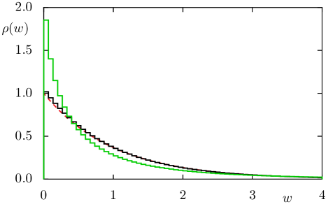
Figure 16: Probability density $\rho(w)$ of the (normalized) off-diagonal matrix elements for the random matrix transition ensemble and coupled kicked rotors for $N=100$. For the random matrix ensemble the (black) histogram matches the exponential quite well, Eq. (33) (red dashed line), as expected. The density for the coupled kicked rotors (green histogram) deviates quite a bit.

The situation is more complicated for the coupled kicked rotors ($N=100$), which after all is an actual dynamical system. The histogram for the kicked rotors deviates quite a bit from the expected exponential behavior. This could be a reflection of a correlation between the matrix elements and eigenvectors, imperfect ergodicity of the system, or the lack of true randomness of the interaction, all of which would generally happen, at least to some extent for a real dynamical system, as opposed to a member of a random matrix ensemble. Nevertheless, for all the derived universal results throughout the paper, the coupled kicked rotors followed the theory quite well. It has long been known within random matrix theory that many results are robust in the sense that deformed ensembles or ones with non-Gaussian matrix elements, or many other kinds of alterations still lead to the same fluctuation properties. It appears that even though the coupled kicked rotors do not approximate a member of the ensemble perfectly, they lead to the same results for the quantities studied in this paper, and thus lie within the range of robustness of the theory.

References

- (1) W. H. Zurek, Decoherence and the transition from quantum to classical, Phys. Today 44, 36 (1991), also see arXiv:quant-ph/0306072.
- (2) W. H. Zurek, Decoherence, einselection, and the quantum origins of the classical, Rev. Mod. Phys. 75, 715 (2003).
- (3) A. Albrecht, Investigating decoherence in a simple system, Phys. Rev. D 46, 5504 (1992).
- (4) P. A. Miller and S. Sarkar, Signatures of chaos in the entanglement of two coupled quantum kicked tops, Phys. Rev. E 60, 1542 (1999).
- (5) H. Fujisaki, T. Miyadera, and A. Tanaka, Dynamical aspects of quantum entanglement for weakly coupled kicked tops, Phys. Rev. E 67, 066201 (2003).
- (6) J. N. Bandyopadhyay and A. Lakshminarayan, Entanglement production in coupled chaotic systems: Case of the kicked tops, Phys. Rev. E 69, 016201 (2004).
- (7) A. Gammal and A. K. Pattanayak, Quantum entropy dynamics for chaotic systems beyond the classical limit, Phys. Rev. E 75, 036221 (2007).
- (8) C. M. Trail, V. Madhok, and I. H. Deutsch, Entanglement and the generation of random states in the quantum chaotic dynamics of kicked coupled tops, Phys. Rev. E 78, 046211 (2008).
- (9) J. M. Deutsch, Quantum statistical mechanics in a closed system, Phys. Rev. A 43, 2046 (1991).
- (10) M. Srednicki, Chaos and quantum thermalization, Phys. Rev. E 50, 888 (1994).
- (11) C. Neill, P. Roushan, M. Fang, Y. Chen, M. Kolodrubetz, Z. Chen, A. Megrant, R. Barends, B. Campbell, B. Chiaro, A. Dunsworth, E. Jeffrey, J. Kelly, J. Mutus, P. J. J. O’Malley, C. Quintana, D. Sank, A. Vainsencher, J. Wenner, T. C. White, A. Polkovnikov, and J. M. Martinis, Ergodic dynamics and thermalization in an isolated quantum system, Nature Physics 12, 1037 (2016).
- (12) L. D’Alessio, Y. Kafri, A. Polkovnikov, and M. Rigol, From quantum chaos and eigenstate thermalization to statistical mechanics and thermodynamics, Adv. Phys. 65, 239 (2016).
- (13) A. I. Larkin and Yu. N. Ovchinnikov, Quasiclassical method in the theory of superconductivity, Sov. Phys. JETP 28, 1200 (1969).
- (14) T. Hartman and J. Maldacena, Time evolution of entanglement entropy from black hole interiors, J. High Energy Phys. 05, 014 (2013).
- (15) N. Lashkari, D. Stanford, M. Hastings, T. Osborne, and P. Hayden, Towards the fast scrambling conjecture, J. High Energy Phys. 04, 022 (2013).
- (16) S. H. Shenker and D. Stanford, Black holes and the butterfly effect, J. High Energy Phys. 03, 067 (2014).
- (17) J. Maldacena, S. H. Shenker, and D. Stanford, A bound on chaos, J. High Energy Phys. 08, 106 (2016).
- (18) D. J. Luitz and Y. Bar Lev, Information propagation in isolated quantum systems, Phys. Rev. B 96, 020406 (2017).
- (19) J. Li, R. Fan, H. Wang, B. Ye, B. Zeng, H. Zhai, X. Peng, and J. Du, Measuring out-of-time-order correlators on a nuclear magnetic resonance quantum simulator, Phys. Rev. X 7, 031011 (2017).
- (20) T. A. Brody, J. Flores, J. B. French, P. A. Mello, A. Pandey, and S. S. M. Wong, Random-matrix physics: spectrum and strength fluctuations, Rev. Mod. Phys. 53, 385 (1981).
- (21) O. Bohigas, M. J. Giannoni, and C. Schmit, Characterization of chaotic quantum spectra and universality of level fluctuation laws, Phys. Rev. Lett. 52, 1 (1984).
- (22) P. A. Lee and A. D. Stone, Universal conductance fluctuations in metals, Phys. Rev. Lett. 55, 1622 (1985).
- (23) B. L. Al’tshuler, Fluctuations in the extrinsic conductivity of disordered conductors, JETP Lett. 41, 648 (1985).
- (24) M. V. Berry, Regular and irregular semiclassical wavefunctions, J. Phys. A 10, 2083 (1977).
- (25) O. Bohigas, S. Tomsovic, and D. Ullmo, Manifestations of classical phase space structures in quantum mechanics, Phys. Rep. 223, 43 (1993).
- (26) S. Tomsovic and D. Ullmo, Chaos-assisted tunneling, Phys. Rev. E 50, 145 (1994).
- (27) A. I. Shnirelman, Ergodic properties of eigenfunctions (in Russian), Usp. Math. Nauk 29, 181 (1974).
- (28) Y. Colin de Verdière, Ergodicité et fonctions propres du laplacien (in French), Commun. Math. Phys. 102, 497 (1985).
- (29) S. Zelditch, Uniform distribution of eigenfunctions on compact hyperbolic surfaces, Duke. Math. J. 55, 919 (1987).
- (30) S. Zelditch and M. Zworski, Ergodicity of eigenfunctions for ergodic billiards, Commun. Math. Phys. 175, 673 (1996).
- (31) A. Bäcker, R. Schubert, and P. Stifter, Rate of quantum ergodicity in euclidean billiards, Phys. Rev. E 57, 5425 (1998), ; erratum ibid. 58 (1998) 5192.
- (32) C. E. Porter (ed.), Statistical Theories of Spectra: Fluctuations, Academic Press, New York (1965).
- (33) P. W. Anderson, Absence of diffusion in certain random lattices, Phys. Rev. 109, 1492 (1958).
- (34) D. M. Basko, I. L. Aleiner, and B. L. Altshuler, Metal–insulator transition in a weakly interacting many-electron system with localized single-particle states, Ann. Phys. (N.Y.) 321, 1126 (2006).
- (35) R. Nandkishore and D. A. Huse, Many-body localization and thermalization in quantum statistical mechanics, Annu. Rev. Condens. Matter Phys. 6, 15 (2015).
- (36) D. A. Abanin and Z. Papić, Recent progress in many-body localization, Ann. Phys. (Berlin) 529, 1700169 (2017).
- (37) A. Pandey and M. L. Mehta, Gaussian ensembles of random Hermitian matrices intermediate between orthogonal and unitary ones, Commun. Math. Phys. 87, 449 (1983).
- (38) J. B. French, V. K. B. Kota, A. Pandey, and S. Tomsovic, Statistical properties of many-particle spectra V. Fluctuations and symmetries, Ann. Phys. (N.Y.) 181, 198 (1988).
- (39) J. B. French, V. K. B. Kota, A. Pandey, and S. Tomsovic, Statistical properties of many-particle spectra VI. Fluctuation bounds on – -noninvariance, Ann. Phys. (N.Y.) 181, 235 (1988).
- (40) P. Hayden, D. Leung, P. W. Shor, and A. Winter, Randomizing quantum states: Constructions and applications, Commun. Math. Phys. 250, 371 (2004).
- (41) P. Hayden, D. W. Leung, and A. Winter, Aspects of generic entanglement, Commun. Math. Phys. 265, 95 (2006).
- (42) C. H. Bennett, H. J. Bernstein, S. Popescu, and B. Schumacher, Concentrating partial entanglement by local operations, Phys. Rev. A 53, 2046 (1996).
- (43) J. Havrda and F. Charvát, Quantification method of classification processes. Concept of structural -entropy, Kybernetika 3, 30 (1967).
- (44) C. Tsallis, Possible generalization of Boltzmann-Gibbs statistics, J. Stat. Phys. 52, 479 (1988).
- (45) I. Bengtsson and K. Życzkowski, Geometry of Quantum States: An Introduction to Quantum Entanglement, Cambridge University Press, Cambridge, England, 1st edition (2006).
- (46) H. Li and F. D. M. Haldane, Entanglement spectrum as a generalization of entanglement entropy: Identification of topological order in non-abelian fractional quantum Hall effect states, Phys. Rev. Lett. 101, 010504 (2008).
- (47) C. Chamon, A. Hamma, and E. R. Mucciolo, Emergent irreversibility and entanglement spectrum statistics, Phys. Rev. Lett. 112, 240501 (2014).
- (48) A. Lakshminarayan, S. C. L. Srivastava, R. Ketzmerick, A. Bäcker, and S. Tomsovic, Entanglement and localization transitions in eigenstates of interacting chaotic systems, Phys. Rev. E 94, 010205(R) (2016).
- (49) M. Horodecki, P. Horodecki, and R. Horodecki, General teleportation channel, singlet fraction, and quasidistillation, Phys. Rev. A 60, 1888 (1999).
- (50) P. Zanardi, C. Zalka, and L. Faoro, Entangling power of quantum evolutions, Phys. Rev. A 62, 030301(R) (2000).
- (51) R. Pal and A. Lakshminarayan, Entangling power of time-evolution operators in integrable and nonintegrable many-body systems, arXiv:1805.11632 [quant-ph] (2018).
- (52) M. A. Nielsen and I. L. Chuang, Quantum Computation and Quantum Information, Cambridge University Press, Cambridge (2010).
- (53) A. Peres, Quantum Theory: Concepts and Methods, Springer Science & Business Media (1995).
- (54) A. Rényi, On measures of entropy and information, in J. Neyman (editor) “Proceedings of the Fourth Berkeley Symposium on Mathematical Statistics and Probability, Volume 1: Contributions to the Theory of Statistics”, 547, Univ. of Calif. Press, Berkeley, Calif. (1961), pp. 547.
- (55) V. A. Marčenko and L. A. Pastur, Distribution of eigenvalues for some sets of random matrices, Math. USSR Sbornik 1, 457 (1967).
- (56) H.-J. Sommers and K. Życzkowski, Statistical properties of random density matrices, J. Phys. A 37, 8457 (2004).
- (57) J. N. Bandyopadhyay and A. Lakshminarayan, Testing statistical bounds on entanglement using quantum chaos, Phys. Rev. Lett. 89, 060402 (2002).
- (58) H. Kubotani, S. Adachi, and M. Toda, Exact formula of the distribution of Schmidt eigenvalues for dynamical formation of entanglement in quantum chaos, Phys. Rev. Lett. 100, 240501 (2008).
- (59) H. Kubotani, S. Adachi, and M. Toda, Measuring dynamical randomness of quantum chaos by statistics of Schmidt eigenvalues, Phys. Rev. E 87, 062921 (2013).
- (60) D. N. Page, Average entropy of a subsystem, Phys. Rev. Lett. 71, 1291 (1993).
- (61) S. Sen, Average entropy of a quantum subsystem, Phys. Rev. Lett. 77, 1 (1996).
- (62) E. Lubkin, Entropy of an -system from its correlation with a -reservoir, J. Math. Phys. 19, 1028 (1978).
- (63) J. B. Keller, Closest unitary, orthogonal and hermitian operators to a given operator, Mathematics Magazine 48, 192 (1975).
- (64) I. S. Gradshteyn, I. M. Ryzhik, D. Zwillinger (ed.), and V. Moll (ed.), Table of Integrals, Series, and Products, Academic Press, Boston, 8th edition (2015).
- (65) K. Bu, U. Singh, L. Zhang, and J. Wu, Average distance of random pure states from maximally entangled and coherent states, arXiv:1603.06715 [quant-ph] (2016).
- (66) A. Lazarides, A. Das, and R. Moessner, Equilibrium states of generic quantum systems subject to periodic driving, Phys. Rev. E 90, 012110 (2014).
- (67) L. D’Alessio and M. Rigol, Long-time behavior of isolated periodically driven interacting lattice systems, Phys. Rev. X 4, 041048 (2014).
- (68) S. Tomsovic, M. B. Johnson, A. C. Hayes, and J. D. Bowman, Statistical theory of parity nonconservation in compound nuclei, Phys. Rev. C 62, 054607 (2000).
- (69) J. Goldberg, U. Smilansky, M. V. Berry, W. Schweizer, G. Wunner, and G. Zeller, The parametric number variance, Nonlinearity 4, 1 (1991).
- (70) M. Michler, A. Bäcker, R. Ketzmerick, H.-J. Stöckmann, and S. Tomsovic, Universal quantum localizing transition of a partial barrier in a chaotic sea, Phys. Rev. Lett. 109, 234101 (2012).
- (71) N. R. Cerruti and S. Tomsovic, A uniform approximation for the fidelity in chaotic systems, J. Phys. A 36, 3451 (2003).
- (72) S. C. L. Srivastava, S. Tomsovic, A. Lakshminarayan, R. Ketzmerick, and A. Bäcker, Universal scaling of spectral fluctuation transitions for interacting chaotic systems, Phys. Rev. Lett. 116, 054101 (2016).
- (73) A. Lakshminarayan, Z. Puchała, and K. Życzkowski, Diagonal unitary entangling gates and contradiagonal quantum states, Phys. Rev. A 90, 032303 (2014).
- (74) T. Tkocz, M. Smaczyński, M. Kuś, O. Zeitouni, and K. Życzkowski, Tensor products of random unitary matrices, Random Matrices: Theory Appl. 1, 1250009 (2012).
- (75) S. Tomsovic, Bounds on the Time-Reversal Noninvariant Nucleon-Nucleon Interaction Derived from Transition Strength Fluctuations, Ph.D. thesis, University of Rochester (1986), [UR Report No. 974, 1987].
- (76) F. Leyvraz and T. H. Seligman, Self-consistent perturbation theory for random matrix ensembles, J. Phys. A 23, 1555 (1990).
- (77) R. Allez and J.-P. Bouchaud, Eigenvector dynamics: General theory and some applications, Phys. Rev. E 86, 046202 (2012).
- (78) F. Benaych-Georges, N. Enriquez, and A. Michaïl, Empirical spectral distribution of a matrix under perturbation, J. Theor. Prob. 1 (2017).
- (79) A. Pandey, Statistical properties of many-particle spectra: III. Ergodic behavior in random-matrix ensembles, Ann. Phys. (N.Y.) 119, 170 (1979).
- (80) J. J. Sakurai and S. F. Tuan, Modern Quantum Mechanics, Addison-Wesley Pub. Co. (1994).
- (81) H. Bruus, C. H. Lewenkopf, and E. R. Mucciolo, Parametric conductance correlation for irregularly shaped quantum dots, Phys. Rev. B 53, 9968 (1996).
- (82) Y. Alhassid and H. Attias, Universal parametric correlations of eigenfunctions in chaotic and disordered systems, Phys. Rev. Lett. 74, 4635 (1995).
- (83) H. Attias and Y. Alhassid, Gaussian random-matrix process and universal parametric correlations in complex systems, Phys. Rev. E 52, 4776 (1995).
- (84) D. Kusnezov and D. Mitchell, Universal predictions for statistical nuclear correlations, Phys. Rev. C 54, 147 (1996).
- (85) A. Lakshminarayan and S. Tomsovic, A degenerate quantum perturbation theory for individual bipartite systems and their statistical properties, in preparation.
- (86) S. C. L. Srivastava, A. Lakshminarayan, S. Tomsovic, and A. Bäcker, Ordered spacing distributions, in preparation.
- (87) V. K. B. Kota, Embedded Random Matrix Ensembles in Quantum Physics, number 884 in Lecture Notes in Physics, Springer International Publishing (2014).
- (88) NIST Digital library of mathematical functions, http://dlmf.nist.gov/, Release 1.0.14 of 2016-12-21, F. W. J. Olver, A. B. Olde Daalhuis, D. W. Lozier, B. I. Schneider, R. F. Boisvert, C. W. Clark, B. R. Miller and B. V. Saunders, (eds.).
- (89) C. Froeschle, On the number of isolating integrals in systems with three degrees of freedom, Astrophys. Space Sci. 14, 110 (1971).
- (90) C. Froeschlé, Numerical study of a four-dimensional mapping, Astron. & Astrophys. 16, 172 (1972).
- (91) B. Gadway, J. Reeves, L. Krinner, and D. Schneble, Evidence for a quantum-to-classical transition in a pair of coupled quantum rotors, Phys. Rev. Lett. 110, 190401 (2013).
- (92) B. V. Chirikov, A universal instability of many-dimensional oscillator systems, Phys. Rep. 52, 263 (1979).
- (93) A. Gorodetski, On stochastic sea of the standard map, Commun. Math. Phys. 309, 155 (2012).
- (94) M. V. Berry, N. L. Balazs, M. Tabor, and A. Voros, Quantum maps, Ann. Phys. (N.Y.) 122, 26 (1979).
- (95) J. H. Hannay and M. V. Berry, Quantization of linear maps on a torus — Fresnel diffraction by a periodic grating, Physica D 1, 267 (1980).
- (96) S.-J. Chang and K.-J. Shi, Evolution and exact eigenstates of a resonant quantum system, Phys. Rev. A 34, 7 (1986).
- (97) J. P. Keating, F. Mezzadri, and J. M. Robbins, Quantum boundary conditions for torus maps, Nonlinearity 12, 579 (1999).
- (98) M. Degli Esposti and S. Graffi, Mathematical aspects of quantum maps, in “The Mathematical Aspects of Quantum Maps”, volume 618 of Lect. Notes Phys., 49, Springer-Verlag, Berlin (2003), pp. 49.
- (99) A. Lakshminarayan, Entangling power of quantized chaotic systems, Phys. Rev. E 64, 036207 (2001).
- (100) M. Richter, S. Lange, A. Bäcker, and R. Ketzmerick, Visualization and comparison of classical structures and quantum states of four-dimensional maps, Phys. Rev. E 89, 022902 (2014).
- (101) D. L. Shepelyansky, Coherent propagation of two interacting particles in a random potential, Phys. Rev. Lett. 73, 2607 (1994).
- (102) M. Žnidarič, Entanglement of random vectors, J. Phys. A 40, F105 (2007).
- (103) S. N. Majumdar, O. Bohigas, and A. Lakshminarayan, Exact minimum eigenvalue distribution of an entangled random pure state, J. Stat. Phys. 131, 33 (2008).
- (104) C. A. Tracy and H. Widom, On orthogonal and symplectic matrix ensembles, Commun. Math. Phys. 177, 727 (1996).
- (105) S. Kumar, B. Sambasivam, and S. Anand, Smallest eigenvalue density for regular or fixed-trace complex Wishart–Laguerre ensemble and entanglement in coupled kicked tops, J. Phys. A 50, 345201 (2017).
- (106) I. Nechita, Asymptotics of random density matrices, Ann. Henri Poincaré 8, 1521 (2007).
- (107) J.-P. Bouchaud and A. Georges, Anomalous diffusion in disordered media: Statistical mechanisms, models and physical applications, Phys. Rep. 195, 127 (1990).
- (108) V. V. Uchaikin and V. M. Zolotarev, Chance and Stability. Stable Distributions and Their Applications, De Gruyter, Berlin, Boston (1999).
- (109) A. Edelman and N. R. Rao, Random matrix theory, Acta Numerica 14, 233 (2005).
- (110) K. Życzkowski and H.-J. Sommers, Induced measures in the space of mixed quantum states, J. Phys. A 34, 7111 (2001).
- (111) S. N. Majumdar and M. Vergassola, Large deviations of the maximum eigenvalue for Wishart and gaussian random matrices, Phys. Rev. Lett. 102, 060601 (2009).
- (112) C. Nadal, S. N. Majumdar, and M. Vergassola, Statistical distribution of quantum entanglement for a random bipartite state, J. Stat. Phys. 142, 403 (2011).
- (113) A. D. Mirlin and F. Evers, Multifractality and critical fluctuations at the Anderson transition, Phys. Rev. B 62, 7920 (2000).
- (114) F. Evers and A. D. Mirlin, Anderson transitions, Rev. Mod. Phys. 80, 1355 (2008).
- (115) E. Bogomolny and O. Giraud, Eigenfunction entropy and spectral compressibility for critical random matrix ensembles, Phys. Rev. Lett. 106, 044101 (2011).
- (116) E. Bogomolny and O. Giraud, Perturbation approach to multifractal dimensions for certain critical random-matrix ensembles, Phys. Rev. E 84, 036212 (2011).
- (117) A. Peres, Quantum Theory: Concepts and Methods, Kluwer Academic Publishers, New York (2002).