Weak lensing power spectrum reconstruction by counting galaxies.– II: Improving the ABS method with the shift parameter

Abstract

In paper I of this series (Yang et al. 2017, ApJ), we proposed an analytical method of blind separation (ABS) to extract the cosmic magnification signal in galaxy number distribution and reconstruct the weak lensing power spectrum. Here we report a new version of the ABS method, with significantly improved performance. This version is characterized by a shift parameter $\mathcal{S}$, with the special case of $\mathcal{S}=0$ corresponding to the original ABS method. We have tested this new version, compared to the previous one, and confirmed its supreme performance in all investigated situations. Therefore it supersedes the previous version. The proof of concept studies presented in this paper demonstrate that it may enable surveys such as LSST and SKA to reconstruct the lensing power spectrum at $z\simeq 1$ with $1\%$ accuracy. We will test with more realistic simulations to verify its applicability in real data.

1. introduction

Gravitational lensing not only distorts galaxy images and induces the cosmic shear effect, but also changes the spatial distribution of galaxies and induces the cosmic magnification effect (Bartelmann, 1995; Bartelmann & Schneider, 2001). This cosmic magnification effect provides a way of lensing measurement alternative to the cosmic shear. However, despite many appealing advantages, its extraction from the overwhelming intrinsic fluctuations of galaxy spatial distribution is highly challenging. Zhang & Pen (2005) pointed out that the two are in principle separable in the flux space, due to their different dependences on galaxy flux. Yang & Zhang (2011); Yang et al. (2015) developed algorithms of implementing this idea at map and power spectrum level, respectively. Both works identified the galaxy stochasticity as the major challenge in this exercise. In principle we can fit the galaxy clustering and the lensing power spectrum simultaneously. However, this induces a model dependence on the galaxy clustering, in particular on its stochastic part. Furthermore, to achieve percent level accuracy, many parameters (such as the scale and flux dependence of deterministic and stochastic bias) should be involved in the fitting. It can be computationally challenging and numerically unstable.

These problems can be overcome by the ABS method developed by two of the authors (Zhang et al., 2016) in the context of CMB foreground removal. Yang et al. (2017) applied the ABS method and demonstrated its applicability. The ABS method does not rely on assumptions of galaxy intrinsic clustering, providing a blind separation of cosmic magnification from galaxy intrinsic clustering. It is computationally fast, since only a few linear algebra operations are needed. The ABS method is exact, when measurement errors (shot noise) in the galaxy clustering measurement is negligible. However, when shot noise exceeds certain level, it may become biased and numerically instable. Similar problem exists in the case of CMB. Recently we have constructed a new version of the ABS method (Zhang et al. (2016), version 2), with a newly introduced shift parameter $\mathcal{S}$. It is also based on exact solutions as the original version, which corresponds to the limit of $\mathcal{S}=0$. The new version solves the problem in CMB foreground removal. A natural step is to apply this new version to cosmic magnification. As will be shown in this paper, the improvement is significant. The ABS reconstructed lensing power spectrum remains unbiased and numerically stable even for cases of large noise. Furthermore, despite of being two independent systems, the same $\mathcal{S}$ works for both CMB and cosmic magnification and therefore no fine tuning is required. We conclude that it should supercede the previous one, and report this new version in the paper II of this series.

2. The new version of ABS with the shift parameter $\mathcal{S}$

Here we briefly summarize the equation that ABS solves in the context of cosmic magnification. For detailes, please refer to paper I. The ABS method solves the following equation,

$$C^{\rm obs}_{ij}=C^{L}_{ij}+\delta C_{ij}^{\rm shot}\ .$$ (1)

$C^{\rm obs}_{ij}$ is the cross power spectrum between the galaxy distribution of the $i$-th and $j$-th flux bins. In this expression, the ensemble average of shot noise power spectrum has been subtracted from the diagonal elements ($i=j$). What left is the residual due to statistical fluctuation, $\delta C_{ij}^{\rm shot}$ ($\langle\delta C_{ij}^{\rm shot}\rangle$). Without loss of generality, we choose flux bins such that different bins have identical error ($\sigma^{2}_{\rm shot}\equiv\langle(\delta C_{ii}^{\rm shot})^{2}\rangle$). $C^{L}_{ij}(\ell)$ is the cross power spectrum between galaxies in the $i$-th and $j$-th flux bins, in the limit of negligible shot noise. This astrophysical signal has three contributions, the intrinsic galaxy auto power spectrum $C_{ij}^{g}$, the cosmic magnification auto power spectrum, and the cross power spectrum between the galaxy intrinsic clustering and cosmic magnification (paper I). As shown in paper I, it can be formulated into the following form,

$$C^{L}_{ij}(\ell)=g_{i}g_{j}\tilde{C}_{\kappa}+\tilde{C}^{g}_{ij}\ .$$ (2)

Here

$$\tilde{C}_{\kappa} \equiv C_{\kappa}(1-r^{2}_{m\kappa})\ .$$ (3)

$C_{\kappa}$ is the lensing power spectrum. $r_{m\kappa}$ is the cross correlation coefficient between lensing and the matter distribution over the redshift range of source galaxies. The prefactor $g(F)$ is determined by $n(F)$, the average number of galaxies per flux interval. For a narrow flux bin, $g=2(\alpha-1)$ where $\alpha\equiv-d\ln n/d\ln F-1$. $\tilde{C}^{g}_{ij}$ is basically the galaxy intrinsic clustering whose exact definition is given in paper I.

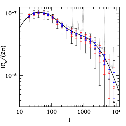
Figure 1.— The improved ABS method with the shift parameter $\mathcal{S}=20\sigma_{\rm shot}$. Errorbars are estimated using $1000$ realizations of shot noise. The 3 sets of data points with errorbars correspond to survey specifications S1, S2 and S3 respectively. Triangle data (black) points with largest errorbars correspond to S1 with smallest galaxy number. Square data (blue) points with smallest errorbars correspond to S3 with highest galaxy number. Open circle data points correspond to S2. For comparison, we overplot the results (dot lines) of the original ABS method ($\mathcal{S}=0$). The previous method breaks when shot noise exceeds certain threshold. In contrast, the new method remains unbiased and numerically stable.

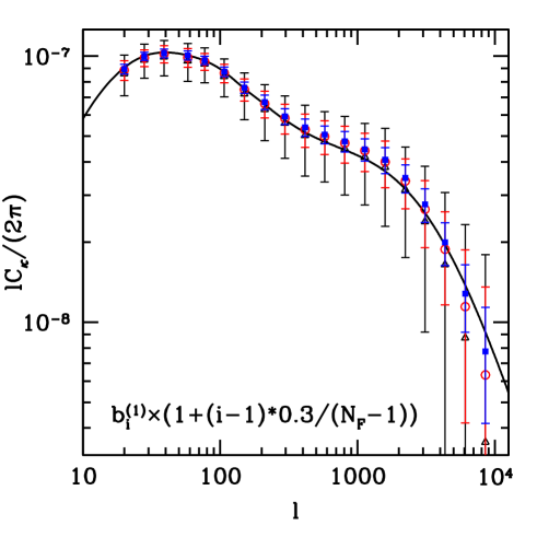
Figure 2.— Similar to Fig. 1, but for case B where the shape of ${\bf b}^{(1)}$ is changed by $30\%$.

The ABS method solves Eq. 1 for $\tilde{C}_{\kappa}$, based on the fact that $g(F)$ is an observable, and its flux dependence differs from that of the galaxy intrinsic clustering. When the number of flux bins is larger than the number of eigenmodes of $C^{g}_{ij}$, the solution to $\tilde{C}_{\kappa}$ is unique and unbiased. Hereafter we will work under this condition. Following the new version of the ABS method (Zhang et al. (2016), version 2), the estimator of $\tilde{C}_{\kappa}$ is

$$\hat{\tilde{C}}_{\kappa}=\left(\sum_{\lambda_{\mu}>\lambda_{\rm cut}\sigma_{\rm shot}}G_{\mu}^{2}\lambda_{\mu}^{-1}\right)^{-1}_{C^{\rm obs}_{ij}+g_{i}g_{j}\mathcal{S}}-\mathcal{S}\ .$$ (4)

Here, $\mathcal{S}$ is the shift parameter of any value. $\lambda_{\mu}$ is the $\mu$-th eigenvalue of the matrix $C^{\rm obs}_{ij}+g_{i}g_{j}\mathcal{S}$. The corresponding eigenvector is ${\bf E}^{(\mu)}$ and $G_{\mu}\equiv{\bf E}^{(\mu)}\cdot{\bf g}$. With the presence of noise, some eigenmodes may be heavily polluted or even completely unphysical. We have to exclude them. Therefore we add a cut and only use eigenmodes with eigenvalue above the threshold $\lambda_{\rm cut}\sigma_{\rm shot}$.

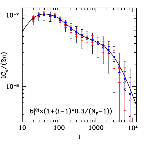
Figure 3.— Similar to Fig. 1, but for case C where the shape of ${\bf b}^{(2)}$ is changed by $30\%$.

Eq. 4 is exact when $\delta C^{\rm shot}_{ij}=0$. In this ideal case, the choice of $\mathcal{S}$ is irrelevant. However, with the presence of measurement error, its choice indeed makes difference. Therefore, $\mathcal{S}$, despite its dimension the same as $\tilde{C}_{\kappa}$, is essentially a regularization parameter associated with the matrix operation. The original ABS method used in paper I is the special case of $\mathcal{S}=0$. However, with the presence of residual shot noise, such version can not pass the null test. In this case, the true signal is zero, while the value returned by the ABS method is always postive. Appropriate choice of $\mathcal{S}$ can solve this problem. Since the first term at the right hand side of Eq. 4 is always positive, $\mathcal{S}$ must be positive in order to pass the null test. Furthermore, it has to satisfy $\mathcal{S}\gg\sigma_{\rm shot}$. Meanwhile, a positive $\mathcal{S}$ improves the numerical stability. When $\mathcal{S}\gg\sigma_{\rm shot}$, it also passes the convergence test. In the context of CMB B-mode foreground removal, we find that $\mathcal{S}=20\sigma^{\rm inst}_{\mathcal{D}}$ is a good choice (Zhang et al. (2016), version 2). It is self-determined within the data through the convergence test and the same choice of $\mathcal{S}$ automatically passes the null test. In this paper, we will adopt the same shift parameter $\mathcal{S}=20\sigma_{\rm shot}$, along with the same cut $\lambda_{\rm cut}=1/2$. These values may not be the optimal choice for lensing reconstruction. However, to avoid fine tunings and uncertainties associated with them, we will fix $\mathcal{S}/\sigma_{\rm shot}=20$ and $\lambda_{\rm cut}=1/2$. Later we will find that the performance of the ABS method with these fixed values is already excellent. Therefore fine tuning in $\mathcal{S}$ and $\lambda_{\rm cut}$ is not required.

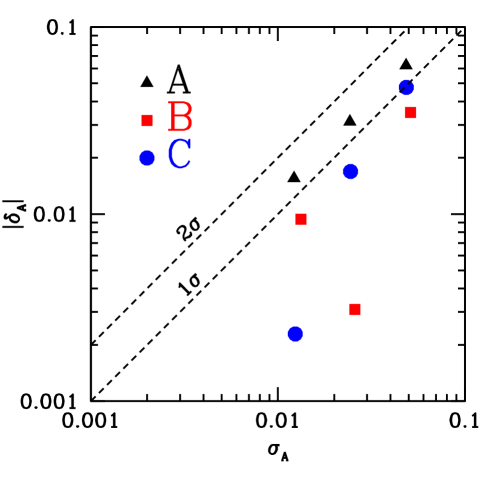
Figure 4.— The systematic error $\delta_{A}$ and statistical error $\sigma_{A}$ in the overall amplitude of the reconstructed lensing power spectrum. Smaller $\sigma_{A}$ corresponds to smaller galaxy number density. Data points of triangle, square and circle are for case A, B & C of galaxy intrinsic clustering, respectively. No systematic error above $1.5\sigma$ confidence level is detected.

3. Test results

We follow the same set up of paper I to test the new ABS method. We adopt 5 flux bins for galaxies in $0.8<z<1.2$. We include both the deterministic and quadratic bias of galaxies. Along with the survey specifications detailed in paper I, this fixes $C^{L}_{ij}$. For each fixed $C^{L}_{ij}$, we generate $1000$ realizations of $\delta C^{\rm shot}_{ij}$, assuming a Gaussian distribution with zero mean and r.m.s. $\sigma_{\rm shot}$. $\sigma_{\rm shot}$ is evaluated adopting the sky coverage $10^{4}$ deg² and the total number of galaxies $N_{\rm tot}$. We adopt the same survey specifications (S1, S2 & S3) as paper I. S1, with $N_{\rm tot}=10^{9}$, resembles a stage IV dark energy survey such as LSST or SKA. S2 has $N_{\rm tot}=5\times 10^{8}$ and S3 has $N_{\rm tot}=2.5\times 10^{8}$. Paper I showed that the performance of ABS depends on both the survey specifications and properties of the galaxy intrinsic clustering. We test different cases of galaxy intrinsic clustering. Case A is the fiducial one, with the linear bias ${\bf b}^{(1)}$ and quadratic bias ${\bf b}^{(2)}$ specified in Fig. 2 of paper I. Case B changes the shape of ${\bf b}^{(1)}$ from faint end to positive end by $30\%$. Case C changes the shape of ${\bf b}^{(2)}$ from faint end to positive end by $30\%$. For case B and C, the previous ABS method shows visible systematic error for some $\ell$ (Fig. 9 & 10, paper I). Therefore we choose to test the new ABS method using them.

Fig. 1 shows the test result for galaxy intrinsic clustering case A. Errorbars are estimated using $1000$ realizations of shot noise ($\delta^{\rm shot}_{ij}$). For the survey specification of lowest galaxy number density (S1), the previous ABS method breaks at $\ell\sim 400$, where significant systematic error and numerical instability develop. Increasing the galaxy number density pushes the scale of failure to higher $\ell$, but the problem remains. In contrast, the new ABS method solves this problem. It remains numerically stable even for large shot noise. It remains unbiased at all scales of interest.

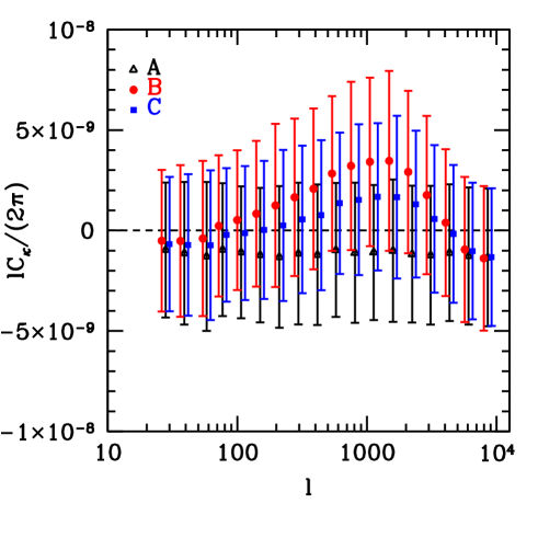
Figure 5.— The null test. We set the input lensing signal as zero and check if the output is consistent with zero. All $3\times 3$ cases investigated pass the null test. For clarity, we only show the results for the survey specification ${\bf S}$1, and shift the data points of set A,B and C horizontally.

Tests on case B (Fig. 2) and C (Fig. 3) show similar improvement on systematic bias and numerical stability. These tests imply that the improvement on systematic bias and numerical stability is general, not limiting to special cases of galaxy intrinsic clustering.

We compress the above results into the statistical error $\sigma_{A}$ and systematic error $\delta_{A}$ in the overall amplitude of the lensing power spectrum. Fig. 4 shows the results for three cases of galaxy number density and three cases of galaxy intrinsic clustering. It shows that the lensing reconstruction by the new ABS method is statistically unbiased at $\sim 1\sigma$ level.

This conclusion is further consolidated by the null test. We set the lensing signal as zero and check whether the ABS output is consistent with zero. For all $3\times 3$ cases above (3 cases of bias by 3 cases of shot noise), the ABS method passes the null test (Fig. 5).

Nevertheless, there are many issues for further investigation when applying the method to real data. We need to deal with survey complexities such as masks, photometric errors and photo-z errors. (1) For masks, we may need to measure the angular correlation functions first. By adopting estimators such as the Landy-Szalay estimator (Landy & Szalay, 1993), the measured correlation functions can be free of masks. We can then Fourier transform them to obtain the power spectra and apply the ABS method to reconstruct the lensing power spectrum. Alternatively, we can directly apply the ABS method to the measured correlation functions and reconstruct the lensing correlation function. (2) We have discussed the photometry calibration error in paper I. The ABS method is applicable with the existence of photometry calibration error, but the r.m.s. must be known. (3) Photo-z errors lead to inaccurate determination of $g$ and therefore impact the reconstruction. However, since the photo-z error for future surveys such as LSST is smaller than the adopted photo-z bin size $\Delta z^{P}=0.4$, this effect is expected to be sub-dominant. We also need more realistic input of galaxy intrinsic clustering, whose stochasticities can go beyond the adopted model of quadratic bias. We are using N-body simulations to generate galaxy mocks with these complexities included, and test the ABS method in a more robust and more realistic way.

4. Conclusions

We report a new version of the ABS method in lensing reconstruction by counting galaxies. With a shift parameter $\mathcal{S}$ about 20 times the measurement noise, the new ABS method significantly improves the systematic bias and numerical stability. For all cases investigated, the new ABS method remains statistically unbiased and numerically stable. Therefore it supersedes the previous version (Yang et al., 2017). When applying to future surveys such as LSST and SKA, it is promising to reconstruct the $z\sim 1$ lensing power spectrum with $1\%$ accuracy. In future works, we will apply this new version of ABS to simulated data and eventually to real data. Both in paper I and the current paper we work on the power spectrum measurement. The ABS method also applies to the correlation functions. We just need to replace the matrix of power spectra in Eq. 4 with the corresponding matrix of cross correlation functions.

References

- Bartelmann (1995) Bartelmann, M. 1995, A&A, 298, 661
- Bartelmann & Schneider (2001) Bartelmann, M., & Schneider, P. 2001, Phys. Rep., 340, 291
- Landy & Szalay (1993) Landy, S. D., & Szalay, A. S. 1993, ApJ, 412, 64
- Yang et al. (2017) Yang, X., Zhang, J., Yu, Y., & Zhang, P. 2017, ApJ, 845, 174
- Yang & Zhang (2011) Yang, X., & Zhang, P. 2011, MNRAS, 415, 3485
- Yang et al. (2015) Yang, X., Zhang, P., Zhang, J., & Yu, Y. 2015, MNRAS, 447, 345
- Zhang & Pen (2005) Zhang, P., & Pen, U.-L. 2005, Physical Review Letters, 95, 241302
- Zhang et al. (2016) Zhang, P., Zhang, J., & Zhang, L. 2016, ArXiv e-prints, arXiv:1608.03707