Policy Optimization With Penalized Point Probability Distance: An Alternative To Proximal Policy Optimization

Abstract

As the most successful variant and improvement for Trust Region Policy Optimization (TRPO), proximal policy optimization (PPO) has been widely applied across various domains with several advantages: efficient data utilization, easy implementation, and good parallelism. In this paper, a first-order gradient reinforcement learning algorithm called Policy Optimization with Penalized Point Probability Distance (POP3D), which is a lower bound to the square of total variance divergence is proposed as another powerful variant. Firstly, we talk about the shortcomings of several commonly used algorithms, by which our method is partly motivated. Secondly, we address to overcome these shortcomings by applying POP3D. Thirdly, we dive into its mechanism from the perspective of solution manifold. Finally, we make quantitative comparisons among several state-of-the-art algorithms based on common benchmarks. Simulation results show that POP3D is highly competitive compared with PPO. Besides, our code is released in https://github.com/paperwithcode/pop3d.

1 Introduction

With the development of deep reinforcement learning, lots of impressive results have been produced in a wide range of fields such as playing Atari game Mnih et al. (2015); Hessel et al. (2017), controlling robotics Lillicrap et al. (2015), Go Silver et al. (2017), neural architecture search Tan et al. (2018); Pham et al. (2018).

The basis of a reinforcement learning algorithm is generalized policy iteration Sutton and Barto (2018), which states two essential iterative steps: policy evaluation and improvement. Among various algorithms, policy gradient is an active branch of reinforcement learning whose foundations are $Policy$ $Gradient$ $Theorem$ and the most classical algorithm REINFORCEMENT Sutton and Barto (2018). Since then, handfuls of policy gradient variants have been proposed, such as Deep Deterministic Policy Gradient (DDPG) Lillicrap et al. (2015), Asynchronous Advantage Actor Critic (A3C) Mnih et al. (2016), Actor Critic using Kronecker-factored Trust Region (ACKTR) Wu et al. (2017), Proximal Policy Optimization (PPO) Schulman et al. (2017).

Improving the strategy monotonically had been nontrivial before the trust region policy optimization(TRPO) was proposed Schulman et al. (2015a). Hessian-free strategy: Fisher vector product is utilized to cut down the computing burden. Specifically, Kullback–Leibler divergence(KLD) acts as a hard constraint in place of objective, because its corresponding coefficient is difficult to set for different problems. However, TRPO still has several drawbacks: too complicated, inefficient data usage. Quite a lot of efforts have been devoted to improving TRPO since then and the most distinguished one is PPO.

PPO can be regarded as a first-order variant of TRPO and have obvious improvements in several facets. In particular, a pessimistic clipped surrogate objective is proposed where TRPO’s hard constraint is replaced by the clipped action probability ratio. In such a way, it constructs an unconstrained optimization problem so that any first-order stochastic gradient optimizer can be directly applied. Besides, it’s easier to be implemented, more robust against various problems and achieves an impressive result on Atari gamesBrockman et al. (2016).

Unfortunately, no further analysis of PPO’s success is provided in that paper. In fact, the pessimistic surrogate objective which is the most critical component of PPO still has some limitations.

As another potential improvement for TRPO and alternative to PPO, this paper focuses on a policy optimization algorithm, where its contributions are:

1. It proposes a simple variant of TRPO called POP3D along with a new surrogate objective containing a point probability penalty item, which is symmetric lower bound to the square of the total variance divergence for two policy distributions. Specifically, it helps to stabilize the learning process and encourage exploration. Furthermore, it escapes from penalty item setting headache along with penalized version TRPO, where is arduous to select one fixed value for various environments.

2. It achieves state-of-the-art results with a clear margin on 49 Atari games within 40 million frame steps based on two shared metrics. Moreover, it also achieves competitive results compared with PPO in the continuous domain.

3. It dives into the mechanism of PPO’s improvement over TRPO by the perspective of solution manifold, which also plays an important role in our method.

4. It enjoys almost all PPO’s advantages such as easy implementation, fast learning ability.

2 Background and Related Works

2.1 Policy Gradient

Agents interact with the environment and receive rewards which are used to adjust their policy in turn. At state ${s_{t}}$, one agent takes strategy $\pi$ and transfers to a new state ${s_{t+1}}$, rewarded ${r_{t}}$ by the environment. Maximizing discounted return (accumulated rewards) $R_{t}$ is its objective. In particular, given a policy $\pi$, $R_{t}$ is defined as

$$R_{t}=\sum_{n=0}^{\infty}(r_{t}+\gamma{r_{t+1}}+\gamma^{2}{r_{t+2}}+...+\gamma^{n}{r_{t+n}}).$$ (1)

$\gamma$ is the discounted coefficient to control future rewards, which lies in the range (0, 1). Regarding a neural network with parameter $\theta$, the policy $\pi_{\theta}(a|s)$ can be learned by maximizing Equation 1 using the back-propagation algorithm. Particularly, given $Q{(s,a)}$ which represents the agent’s return in state $s$ after taking action $a$, the objective function can be written as

$$\max_{\theta}\quad E_{s,a}\log\pi_{\theta}(a|s)Q(s,a).$$ (2)

Equation 2 lays the foundation for handfuls of policy gradient based algorithms, Another variant can be deduced by using

$$A(s,a)=Q(s,a)-V(s)$$ (3)

to replace $Q(s,a)$ in Equation 2 equivalently, $V(s)$ can be any function so long as $V$ depends on $s$ but not $a$. In most cases, state value function is used for $V$, which not only helps to reduce variations but has clear physical meaning. Formally, it can be written as

$$\max_{\theta}\quad E_{s,a}\log\pi_{\theta}(a|s)A(s,a).$$ (4)

2.2 Advantage Estimate

One commonly used method for advantage calculation is one step estimation, which estimates

$$\begin{split}A(s_{t},a)&=Q(s_{t},a)-V(s_{t})\\ &=r_{t}+\gamma V(s_{t+1})-V(s_{t}).\end{split}$$ (5)

A better estimate for advantage called generalized advantage estimation is proposed in Schulman et al. (2015b), where one, two, three, up to $\infty$ time step estimate are combined and summarized using $\lambda$ based weights, which helps to estimate more accurately. The generalized advantage estimator is defined as

$$\begin{split}\hat{A}_{t}^{GAE(\gamma,\lambda)}&=\sum_{l=0}^{\infty}(\gamma\lambda)^{l}\delta_{t+l}^{V}\\ \delta_{t+l}^{V}&=r_{t+l}+\gamma V(s_{t+l+1})-V(s_{t+l}).\end{split}$$ (6)

The parameter $\lambda$ meets $0\leq\lambda\leq 1$, which controls the trade-off between bias and variance.

2.3 Trust Region Policy Optimization

Schulman et al. propose TRPO to update the policy monotonically. In particular, its mathematical form is

$$\begin{split}\max_{\theta}\quad&E_{t}[\frac{\pi_{\theta}(a_{t}|s_{t})}{\pi_{\theta_{old}}(a_{t}|s_{t})}\hat{A_{t}}]\\ -&CE_{t}[KL[\pi_{\theta_{old}}(\cdot|s_{t}),\pi_{\theta}(\cdot|s_{t})]]\\ C&=\frac{2\epsilon\gamma}{(1-\gamma)^{2}}\\ \epsilon&=\max_{s}E_{a\sim\pi_{\theta}(a|s)}[A_{\pi_{\theta_{old}}}(s,a)]),\end{split}$$ (7)

where $C$ is the penalty coefficient.

In practice, the policy update steps would be too small if $C$ is valued as Equation 7. In fact, it’s intractable to calculate $C$ beforehand since it requires traversing all states to reach the maximum. Moreover, inevitable bias and variance will be introduced by estimating the advantages of old policy while training. Instead, a surrogate objective is maximized based on the KLD constraint between the old and new policy, which can be written as below,

$$\begin{split}\max_{\theta}\quad&E_{t}[\frac{\pi_{\theta}(a_{t}|s_{t})}{\pi_{\theta_{old}}(a_{t}|s_{t})}\hat{A_{t}}]\\ s.t.\quad&E_{t}[KL[\pi_{\theta_{old}}(\cdot|s_{t}),\pi_{\theta}(\cdot|s_{t})]]\leq\delta\end{split}$$ (8)

where $\delta$ is the KLD upper limitation. In addition, the conjugate gradient algorithm is applied to solve Equation 8 more efficiently. Two major problems have yet to be addressed: one is its complexity even using the conjugate gradient approach, another is compatibility with architectures that involve noise or parameter sharing tricks Schulman et al. (2017).

2.4 Proximal Policy Optimization

To overcome the shortcomings of TRPO, PPO replaces the original constrained problem with a pessimistic clipped surrogate objective where KL constraint is implicitly imposed. The loss function can be written as

$$\begin{split}L^{CLIP}(\theta)&=E_{t}[\min(r_{t}(\theta)\hat{A_{t}},\\ &clip(r_{t}(\theta),1-\epsilon,1+\epsilon)\hat{A_{t}})]\\ &r_{t}(\theta)=\frac{\pi_{\theta}(a_{t}|s_{t})}{\pi_{\theta_{old}}(a_{t}|s_{t})}_{,}\end{split}$$ (9)

where $\epsilon$ is a hyper-parameter to control the clipping ratio. Except for the clipped PPO version, KL penalty versions including fixed and adaptive KLD. Besides, their simulation results convince that clipped PPO performs best with an obvious margin across various domains.

3 Policy Optimization with Penalized Point Probability Distance

Before diving into the details of POP3D, we review some drawbacks of several methods, which partly motivate us.

3.1 Disadvantages of Kullback-Leibler Divergence

According to Theorem 1 in TRPO paper, the following inequality holds.

$$\begin{split}\eta(\pi_{\theta})&\leq L_{\pi_{\theta_{old}}}(\pi_{\theta})+\frac{2\epsilon\gamma}{(1-\gamma)^{2}}\alpha^{2}\\ \alpha&=D_{TV}^{\max}(\pi_{\theta_{old}},\pi_{\theta})\\ D_{TV}^{\max}(\pi_{\theta_{old}},\pi_{\theta})&=\max_{s}D_{TV}(\pi_{\theta_{old}}||\pi_{\theta})\end{split}$$ (10)

TRPO replaces the square of total variation divergence $D_{TV}^{max}(\pi_{\theta_{old}},\pi_{\theta})$ by $D_{KL}^{\max}(\pi_{\theta_{old}},\pi_{\theta})=\max_{s}D_{KL}(\pi_{\theta_{old}}||\pi_{\theta})$. Given a discrete distribution $p$ and $q$, their total variation divergence $D_{TV}(p||q)$ is defined by $\frac{1}{2}\sum_{i}|p_{i}-q_{i}|$. Obviously, $D_{TV}$ is symmetric by definition, while KLD is asymmetric.

Formally, given state $s$, KLD of $\pi_{\theta_{old}}(\cdot|s)$ for $\pi_{\theta}(\cdot|s)$ can be written as

$$\begin{split}D_{KL}(\pi_{\theta_{old}}(\cdot|s)||\pi_{\theta}(\cdot|s))&=\sum_{a}{}\pi_{\theta_{old}}(a|s)\\ &\ln\frac{\pi_{\theta_{old}}(a|s)}{\pi_{\theta}(a|s)}.\end{split}$$ (11)

Similarly, KLD in the continuous domain can be defined simply by replacing summation with integration.

The consequence of KLD’s asymmetry leads to a non-negligible difference of whether choose $D_{KL}(\pi_{\theta_{old}}||\pi_{\theta})$ or $D_{KL}(\pi_{\theta}||\pi_{\theta_{old}})$. Sometimes, those two choices result in quite different solutions. Robert compared the forward and reverse KL on a distribution, one solution matches only one of the modes, and another covers both modes Robert (2014). Therefore, KLD is not an ideal bound or approximation for the expected discounted cost.

3.2 Discussion about Pessimistic Proximal Policy

In fact, PPO is called pessimistic proximal policy optimization in the meaning of its objective construction style.

Without loss of generality, supposing ${A_{t}}>0$ for given state $s_{t}$ and action $a_{t}$, and the optimal choice is $a_{t}^{\star}$. When $a_{t}=a_{t}^{\star}$, a good update policy is to increase the probability of action to a relatively high value $a_{t}^{\star}$ by adjusting $\theta$. However, the clipped item $clip(r_{t}(\theta),1-\epsilon,1+\epsilon)\hat{A_{t}}$ will fully contribute to the loss function by the minimum operation, which ignores further reward by zero gradients even though it’s the optimal action. Other situation with ${A_{t}}<0$ can be analyzed in the same manner.

However, if the pessimistic limitation is removed, PPO’s performance decreases dramatically Schulman et al. (2017), which is again confirmed by our preliminary experiments. In a word, the pessimistic mechanism plays a very critical role for PPO by a relatively weak preference for good action decision for a given state, which in turn affects learning efficiency.

3.3 Restricted Solution Manifold

To be simple, we don’t take the model identifiability issues along with deep neural network into account here because they don’t affect the following discussion much Goodfellow et al. (2016). Suppose $\pi_{\theta\star}$ is the optimal solution for a given environment, in most cases, more than one parameter set for $\theta$ can generate the ideal policy, especially when $\pi_{\theta\star}$ is learned by a deep neural network. In other words, the relationship between $\theta$ and $\pi_{\theta\star}$ is many to one. On the other hand, when agents interact with the environment using policy represented by neural networks, the action is taken approximately strongly corrected with the highest probability value. Although some strategies of enhancing exploration are applied, they don’t affect the policy much in the meaning of expectation.

Taking the Atari-Pong game for example, when an agent sees a Pong ball is coming nearly, its optimal policy is moving the racket to the right position. The probability of this action is a relatively high value such as 0.95 and it’s near to impossible that this value is 1.0 since it’s produced by a softmax operation on the several discrete actions. In fact, we hardly obtained the optimal solution accurately, instead, our goal is a good enough answer. Namely, $\theta_{1}$ outputting a probability 0.95 and $\theta_{2}$ with 0.9 for the right action are both good answers. During the training process, these similar events occur frequently.

Using a penalty such as KLD cannot handle it effectively, because it involves all of the actions’ probabilities. Moreover, it doesn’t stop penalizing unless two distributions become exactly indifferent or the advantage item is large enough to compensate for the KLD cost. Therefore, even if $\theta$ outputs $\theta_{old}$ the same high probability for the right action, it’s still penalized owing to probabilities mismatch for other uncritical actions. Indeed, when a person is asked to make the choice, corresponding action will be taken only if the probability is above a threshold. From the perspective of the manifold, if the optimal parameters constitute a solution manifold. The KLD penalty will act until $\theta$ exactly locates in the solution if possible. However, if the agent concentrates only on critical actions like a human, it’s much easier to approach the manifold, which in fact, expands the solution manifold at least one dimension such as curves to surfaces and surfaces to spheres at best.

Besides, since mini-batch is a commonly used trick for training neural networks, removing this unexpected penalty helps to decrease penalty noises, which are reflected by the corresponding gradient.

3.4 Exploration

One shared highlight in reinforcement learning is the balance between exploitation and exploration. For a policy-gradient algorithm, entropy is added in the total loss to encourage exploration in most case. When included in loss function, KLD penalizes the old and new policy probability mismatch for all possible actions as Equation 11. This strict punishment for every action’s probability mismatch, which discourages exploration.

3.5 Point Probability Distance

To overcome the above-mentioned shortcomings, we propose a surrogate objective with the point probability distance penalty, which is symmetric and more optimistic than PPO. In the discrete domain, when the agent takes action $a$, the point probability distance between $\pi_{\theta_{old}}(\cdot|s)$ and $\pi_{\theta}(\cdot|s)$ is defined by

$$\begin{split}D_{pp}(\pi_{\theta_{old}}(\cdot|s),\pi_{\theta}(\cdot|s))&=({\pi_{\theta_{old}}(a|s)}\\ &-{\pi_{\theta}(a|s)})^{2}.\end{split}$$ (12)

Attention should be paid to the penalty definition item, the distance is measured by the point probability, which emphasizes its mismatch for the sampled actions for a state. Undoubtedly, $D_{pp}$ is symmetry by definition. Furthermore, it can be proved that $D_{pp}$ is indeed a lower bound for the total variance divergence $D_{TV}$. As a special case, it can be easily proved that for binary distribution, $D_{TV}^{2}(p||q)=D_{pp}(p||q)$.

Theorem 1

For two discrete probability distributions p and q with $K$ values, then $D_{TV}^{2}(p||q)\geq D_{pp}(p||q)$ holds.

Proof 1

Let $a=p_{l},b=q_{l}$ for any $l$, and suppose $a\geq b$ without loss of generalization. So,

$$D_{TV}^{2}(p||q) = (\frac{1}{2}\sum_{i=1}^{K}|p_{i}-q_{i}|)^{2}$$

$$= (\frac{1}{2}\sum_{i=1,i\neq l}^{K}|p_{i}-q_{i}|+\frac{1}{2}|p_{l}-q_{l}|)^{2}$$

$$\geq (\frac{1}{2}|\sum_{i=1,i\neq l}^{K}p_{i}-q_{i}|+\frac{1}{2}(a-b))^{2}$$

$$= (\frac{1}{2}|1-a-(1-b)|+\frac{1}{2}(a-b))^{2}$$

$$= (\frac{1}{2}(a-b)+\frac{1}{2}(a-b))^{2}$$

$$= D_{pp}(p||q)$$

Q.E.D.

Since $0\leq{\pi_{\theta}(a|s)}\leq 1$ holds for discrete action space, $D_{pp}$ has a lower and upper boundary: $0\leq D_{pp}\leq 1$. Moreover, $D_{pp}$ is less sensitive to action space dimension than KLD, which has a similar effect as PPO’s clipped ratio to increase robustness and enhance stability.

Equation 12 stays unchanged for the continuous domain, and the only difference is $\pi_{\theta}(a|s)$ represents point probability density instead of probability.

3.6 POP3D

After we have defined the point probability distance, we use a new surrogate objective for POP3D, which can be written as

$$\begin{split}\max_{\theta}\quad&E_{t}[\frac{\pi_{\theta}(a_{t}|s_{t})}{\pi_{\theta_{old}}(a_{t}|s_{t})}\hat{A_{t}}-\\ \quad&\beta D_{pp}(\pi_{\theta_{old}}(\cdot|s),\pi_{\theta}(\cdot|s))],\end{split}$$ (13)

where $\beta$ is the penalized coefficient. These combined advantages lead to considerable performance improvement, which escapes from the dilemma of choosing preferable penalty coefficient. Besides, we use generalized advantage estimates to calculate $\hat{A_{t}}$. Algorithm 1 shows the complete iteration process of POP3D. Moreover, it possesses the same computing cost and data efficiency as PPO.

Algorithm 1 POP3D

1:  Input: max iterations $L$ , actors $N$, epochs $K$

2:  for $iteration=1$ to $L$ do

3:     for $actor=1$ to $N$ do

4:        Run policy $\pi_{\theta_{old}}$ for $T$ time steps

5:        Compute advantage estimations $\hat{A}_{1},...,\hat{A}_{T}$

6:     end for

7:     for $epoch=1$ to $K$ do

8:        Optimized loss objective wrt $\theta$ with mini-batch size $M\leq NT$, then update $\theta_{old}\leftarrow\theta$.

9:     end for

10:  end for

3.7 Relationship With PPO

To conclude this section, we take some time to see why PPO works by taking the above viewpoints into account.

When we pour more attention to Equation 9, the ratio $r_{t}(\theta)$ only involves the probability for given action $a$, which is chosen by policy $\pi$. In other words, all other actions’ probabilities except $a$ are not activated, which no longer contribute to back-propagation and allow probability mismatch. Obviously, this procedure behaves similarly as POP3D, which expands the restricted solution manifold.

Above all, POP3D is designed to conform with the regulations for overcoming above mentioned problems, and in the next section experiments from commonly used benchmarks will evaluate its performance.

4 Experiments

4.1 Controlled Experiments Setup

OpenAI Gym is a well-known simulation environment to test and evaluate various reinforcement algorithms, which is composed of both discrete (Atari) and continuous (Mujoco) domains Brockman et al. (2016). Most of recent deep reinforcement learning methods such as DQN variants Van Hasselt et al. (2016); Wang et al. (2015); Schaul et al. (2015); Bellemare et al. (2017); Hessel et al. (2017), A3C, ACKTR, PPO are evaluated using only one set of hyper-parameters. Therefore, we evaluate POP3D’s performance on 49 Atari games(v4, discrete action space ) and 7 Mujoco(v2, continuous space).

Since PPO is a distinguished RL algorithm which defeats various methods such as A3C, A2C ACKTR, we focus on a detailed quantitative comparison with fine-tuned PPO. And we don’t consider large scale distributed algorithms Apex-DQN Horgan et al. (2018) and IMPALA Espeholt et al. (2018), because we concentrate on comparable and fair evaluation, while the latter is designed to apply with large scale parallelism. Nevertheless, some orthogonal improvements from those methods have the potentials to improve our method further. Furthermore, we include TRPO to acts as a baseline method. In addition, quantitative comparisons between KLD and point probability penalty helps to convince the critical role of the latter, where the former strategy is named fixed KLD in Schulman et al. (2017) and can act as another good baseline in this context, named by BASELINE below.

In particular, we retrained one agent for each game with fine-tuned hyper-parameters. To avoid the problems of reproduction about reinforcement algorithms mentioned in Henderson et al. (2017), we take the following measures:

• Use the same training steps and make use of the same amount of game frames(40M for Atari game and 10M for Mujoco).

• Use the same neural network structures, which is CNN model with one action head and one value head for Atari game, and fully-connected model with one value head and one action head which produces the mean and standard deviation of diagonal Gaussian distribution as PPO.

• Initialize parameters using the same strategy as PPO.

• Keep Gym wrappers from Deepmind such as reward clipping and frame stacking unchanged for Atari domain, and enable 30 no-ops at the beginning of each episode.

• Use Adam optimizer Kingma and Ba (2014) and decrease $\alpha$ linearly from 1 to 0 for Atari domain as PPO.

To facilitate further comparisons with other approaches, we release the seeds and detailed results(across the entire training process for different trials). In addition, we randomly select three seeds from {0, 10, 100, 1000, 10000} for two domains, {10,100,1000} for Atari and {0,10,100} for Mujoco in order to decrease unfavorable subjective bias stated in Henderson et al. (2017).

4.2 Evaluation Metrics

PPO utilizes two score metrics for evaluating agents performance using various RL algorithms. One is the mean score of last 100 episodes $Score_{100}$, which measures how high a strategy can hit eventually. Another is the average score across all episodes $Score_{all}$, which evaluates how fast an agent learns. In this paper, we conform to this routine and calculate individual metric by averaging three seeds in the same way.

4.3 Discrete Domain Comparisons

4.3.1 Hyper-parameters

We search hyper-parameter four times for the penalty coefficient $\beta$ based on four Atari games while keeping other hyper-parameters unchanged as PPO and fix $\beta=5.0$ to train all Atari games. For BASELINE, we also search hyper-parameter four times on penalty coefficient $\beta$ and choose $\beta=10.0$. To save space, detailed hyper-parameter setting can be found in Table  4, 5 and 6.

This process is not beneficial for POP3D owing to missing optimization for all hyper-parameters. There are two reasons to make this choice. On the one hand, it’s the simplest way to make a relatively fair comparison group such as keeping the same iterations and epochs within one loop to our knowledge. On the other hand, this process imposes low search requirements for time and resource. That’s to say, we can draw a conclusion that our method is at least competitive to PPO if it performs better on benchmarks.

4.3.2 Comparison Results

The final score of each game is averaged by three different seeds and the highest is in bold. As Table 1 shows, POP3D outperforms 32 across 49 Atari games in view of the final score, followed by PPO with 11, BASELINE with 5 and TRPO with 1. Interestingly, for games that POP3D score highest, BASELINE score worse than PPO more often than the other way round, which means that POP3D is not just an approximate version of BASELINE.

For another metric, POP3D wins 20 out of 49 Atari games which matches PPO with 18, followed by BASELINE with 6, and last ranked by TRPO with 5.

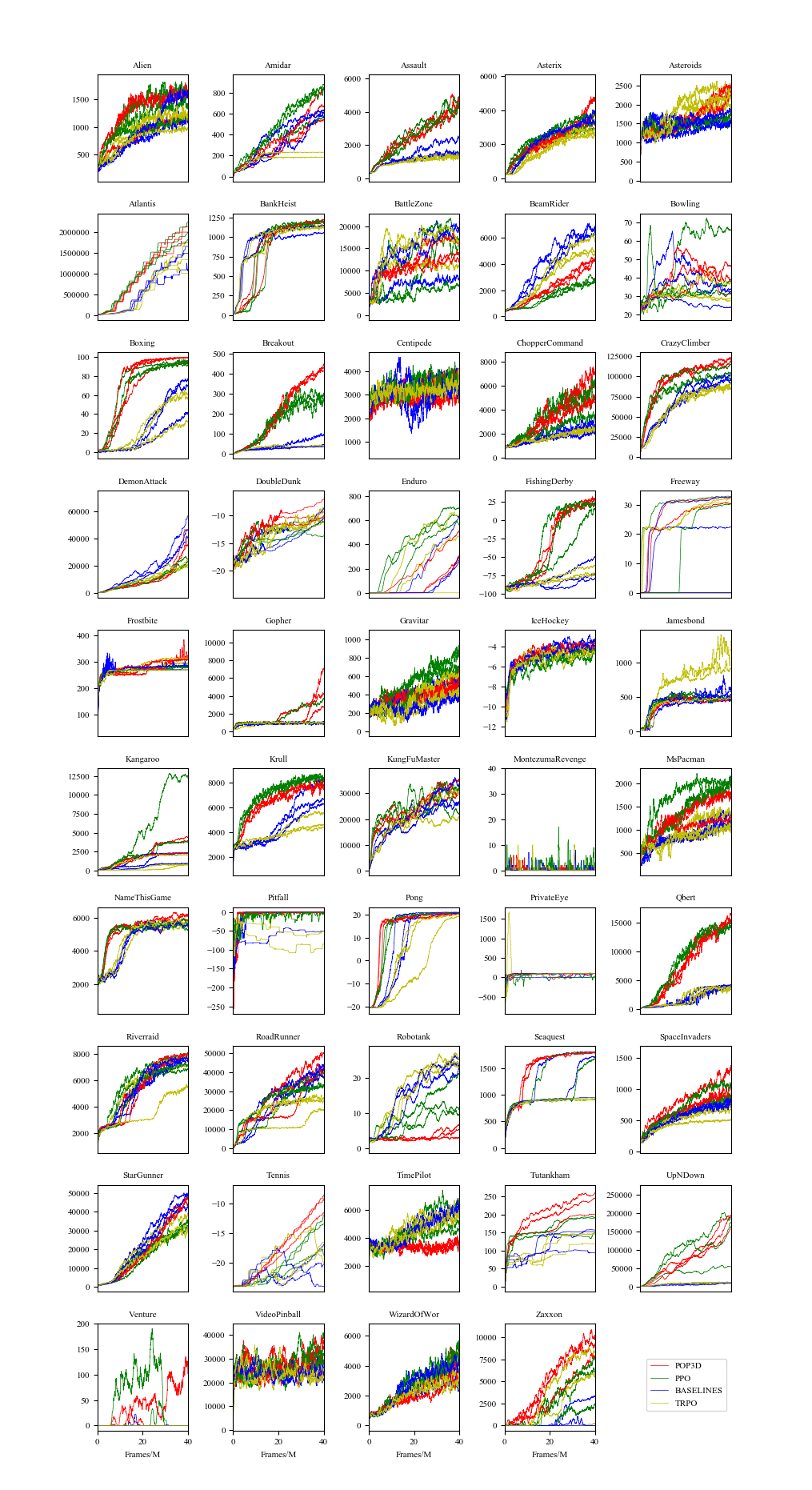
Figure 1: Score curves of three methods on 49 Atari games within 40 million frame steps.

Detailed performance during the whole training process can be found in Figure 1. If we measure the stability of an algorithm by the score variance of different trials, POP3D scores high with good stability across various seeds. And PPO behaves worse in Game Kangaroo and UpNDown. Interestingly, BASELINE shows a large variance for different seeds for several games such as BattleZone, Freeway, Pitfall and Seaquest.

In sum, POP3D reveals its better capacity to score high and similar fast learning ability in this domain. The detailed metric for each game is listed in Table 3 and  9.

Metric	PPO	POP3D	BASELINE	TRPO
$Score_{100}$	11	32	5	1
$Score_{all}$	18	20	6	5

Table 1: The number of games ”won” by each algorithm for Atari game, where the score metric is averaged on three seeds.

4.4 Continuous Domain Comparisons

In this section, we focus on comparisons between POP3D and PPO in Mujoco domain.

4.4.1 Hyper-parameters

For PPO, we use the same hyper-parameter configuration as Schulman et al. (2017). Regarding POP3D, we search on two games three times and select 5.0 as the penalty coefficient. More details about hyper-parameters for PPO and POP3D are listed in Table 7 and  8 of Section  A.2. Unlike the Atari domain, we we utilize the constant learning rate strategy as Schulman et al. (2017) in the continuous domain instead of the linear decrease strategy.

4.4.2 Comparison Results

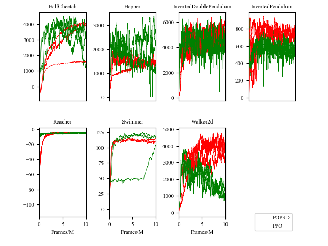
Figure 2: Score curves of three methods on 7 Mujoco games within 10 million frame steps.

The scores are also averaged on three trials and summarized in Table 2. POP3D occupies 5 out of 7 games on $Score_{100}$, and 3 on $Score_{all}$. Evaluation metrics of both across different games are illustrated in Table 10 and 11. Each algorithm’s score performance with iteration steps is shown in Figure 2.

Metric	PPO	POP3D
$Score_{100}$	2	5
$Score_{all}$	4	3

Table 2: The number of games won by each algorithm for Mujoco game, where the score metric is averaged on three seeds.

game	POP3D	PPO	BASELINE	TPRO
Alien	1510.80	1431.17	1311.23	1110.40
Amidar	729.15	790.75	655.10	200.56
Assault	5400.13	4438.82	1846.75	1363.46
Asterix	4310.67	3483.17	3657.67	2651.33
Asteroids	2488.10	1605.33	1615.37	2205.70
Atlantis	2193605.67	2140536.33	1515993.33	1419104.67
BankHeist	1212.23	1206.67	1124.43	1125.17
BattleZone	15466.67	14766.67	14690.00	15123.33
BeamRider	4549.00	2624.19	6898.09	5073.75
Bowling	38.99	47.27	30.48	31.24
Boxing	97.23	93.70	65.33	50.07
Breakout	458.41	281.93	67.70	40.65
Centipede	3315.44	3565.18	3393.93	3353.14
Chopper-
Command	6308.33	4872.67	2676.00	2286.67
CrazyClimber	120247.33	105940.00	98219.67	87522.33
DemonAttack	61147.33	26740.57	57476.65	21525.08
DoubleDunk	-7.89	-11.22	-8.61	-10.04
Enduro	459.85	698.46	518.41	365.95
FishingDerby	28.99	17.72	-64.27	-69.64
Freeway	21.21	21.11	18.37	20.89
Frostbite	316.87	280.30	280.30	291.77
Gopher	6207.00	1791.00	940.87	938.27
Gravitar	557.17	753.50	449.00	495.17
IceHockey	-4.12	-4.83	-3.61	-4.61
Jamesbond	527.17	488.17	685.17	901.67
Kangaroo	3891.67	6845.00	1850.00	1214.67
Krull	7715.68	8329.08	7204.95	4881.65
KungFuMaster	33728.00	29958.67	29843.67	26808.00
Montezuma-
Revenge	0.00	10.67	0.67	0.00
MsPacman	1683.87	1981.50	1170.70	1133.57
NameThisGame	6065.63	5397.47	5672.60	5604.10
Pitfall	0.00	-2.32	-17.26	-43.60
Pong	20.50	20.80	20.79	19.63
PrivateEye	79.67	36.50	99.67	99.33
Qbert	15396.67	14556.83	4114.00	3781.58
Riverraid	8052.23	7360.40	7722.00	6773.67
RoadRunner	44679.67	36289.33	43626.33	24061.33
Robotank	4.60	14.15	24.60	24.18
Seaquest	1807.47	1470.60	1501.47	926.40
SpaceInvaders	1216.15	944.63	814.53	634.07
StarGunner	48984.00	33862.00	47738.00	33442.67
Tennis	-8.32	-13.74	-19.13	-18.40
TimePilot	3770.33	5321.33	6278.33	5701.00
Tutankham	241.21	177.58	135.80	136.21
UpNDown	242701.51	153160.66	11815.87	10949.53
Venture	36.33	0.00	4.00	0.00
VideoPinball	37780.70	31577.24	21438.64	25095.20
WizardOfWor	4704.00	4886.67	3533.67	3103.00
Zaxxon	9472.00	5728.67	1179.67	4796.67

Table 3: Mean final scores (last 100 episodes) of PPO, POP3D, BASELINE and TRPO on Atari games after 40M frames. The results are averaged on three trials.

In summary, both metrics indicates that POP3D is competitive to PPO in the continuous domain.

5 Conclusion

In this paper, we introduce a new reinforcement learning algorithm called POP3D (Policy Optimization with Penalized Point Probability Distance), which acts as a TRPO variant like PPO. Compared with KLD that is an upper bound for the square of total variance divergence between two distributions, the penalized point probability distance is a symmetric lower bound. Besides, it equivalently expands the optimal solution manifold effectively while encouraging exploration, which is a similar mechanism implicitly possessed by PPO. The proposed method not only possesses several critical improvements from PPO but outperforms with a clear margin on 49 Atari games from the respective of final scores and meets PPO’s match as for fast learning ability.

More interestingly, it not only suffers less from the penalty item setting headache along with TRPO, where is arduous to select one fixed value for various environments, but outperforms fixed KLD baseline from PPO. In summary, POP3D is highly competitive and an alternative to PPO.

Appendix A Hyper-parameters

A.1 Atari

PPO’s and POP3D’s hyper-parameters for Mujoco game are respectively listed in Table 4 and 5.

Hyper-parameter	Value
Horizon (T)	128
Adam step-size	2.5 $\times 10^{-4}\times\alpha$
Num epochs	3
Mini-batch size	32$\times 8$
Discount $(\gamma)$	0.99
GAE parameter $(\lambda)$	0.95
Number of actors	8
Clipping parameter	0.1$\times\alpha$
VF coeff.	1
Entropy coeff.	0.01

Table 4: PPO’s hyper-parameters for Atari game.

Hyper-parameter	Value
Horizon (T)	128
Adam step-size	2.5 $\times 10^{-4}\times\alpha$
Num epochs	3
Mini-batch size	32$\times 8$
Discount $(\gamma)$	0.99
GAE parameter $(\lambda)$	0.95
Number of actors	8
VF coeff.	1
Entropy coeff.	0.01
KL penalty coeff.	5.0

Table 5: POP3D’s hyper-parameters for Atari game.

Hyper-parameter	Value
Horizon (T)	128
Adam step-size	2.5 $\times 10^{-4}\times\alpha$
Num epochs	3
Mini-batch size	32$\times 8$
Discount $(\gamma)$	0.99
GAE parameter $(\lambda)$	0.95
Number of actors	8
VF coeff.	1
Entropy coeff.	0.01
KL penalty coeff.	10.0

Table 6: BASELINE’s hyper-parameters for Atari game.

A.2 Mujoco

PPO’s and POP3D’s hyper-parameters for Mujoco game are respectively listed in Table 7 and 8.

Hyper-parameter	Value
Horizon (T)	2048
Adam step-size	3 $\times 10^{-4}$
Num epochs	10
Mini-batch size	64
Discount $(\gamma)$	0.99
GAE parameter $(\lambda)$	0.95
Clipping parameter	0.2

Table 7: PPO’s hyper-parameters for Mujoco game.

Hyper-parameter	Value
Horizon (T)	2048
Adam step-size	3 $\times 10^{-4}$
Num epochs	10
Mini-batch size	64
Discount $(\gamma)$	0.99
GAE parameter $(\lambda)$	0.95
KL penalty coeff.	5.0

Table 8: POP3D’s hyper-parameters for Mujoco game.

Appendix B Score Tables and Curves

Mean scores of various methods for Atari domain are listed in Table 9.

game	POP3D	PPO	BASELINE	TRPO
Alien	1147.29	1115.94	851.13	841.08
Amidar	299.55	413.46	295.91	169.12
Assault	2139.15	2168.93	1159.50	971.78
Asterix	2004.43	2102.10	1884.68	1342.83
Asteroids	1652.48	1470.46	1477.71	1760.73
Atlantis	488134.03	596807.27	192798.74	174394.94
BankHeist	662.26	643.94	859.25	831.95
BattleZone	11131.44	9387.77	11674.30	12918.39
BeamRider	1965.27	1460.59	3321.25	2431.63
Bowling	37.97	39.41	33.90	30.99
Boxing	83.12	78.61	27.92	23.07
Breakout	143.60	124.98	29.99	26.56
Centipede	3056.81	3344.63	3042.48	3142.22
Chopper-
Command	3269.47	3106.14	1780.38	1595.82
CrazyClimber	97257.52	90169.60	69258.31	63189.78
DemonAttack	7611.27	7180.43	9814.42	6204.68
DoubleDunk	-13.70	-15.45	-15.93	-14.57
Enduro	107.84	321.20	92.59	140.67
FishingDerby	-21.00	-27.51	-81.90	-81.97
Freeway	17.76	15.87	15.93	17.33
Frostbite	276.47	267.73	270.42	270.57
Gopher	1556.29	1196.20	900.74	875.93
Gravitar	413.20	509.81	342.74	317.86
IceHockey	-4.67	-5.50	-4.61	-5.21
Jamesbond	358.54	394.45	380.91	519.01
Kangaroo	1614.63	2199.74	937.98	566.85
Krull	6538.16	7195.24	4760.66	3861.87
KungFuMaster	23253.96	23283.31	19637.58	18293.12
Montezuma-
Revenge	0.14	0.74	0.22	0.12
MsPacman	1214.09	1482.77	860.63	864.84
NameThisGame	5353.14	5199.37	4562.32	4504.67
Pitfall	-2.41	-5.81	-31.27	-33.93
Pong	13.24	12.83	7.20	-2.91
PrivateEye	87.37	52.76	56.70	98.79
Qbert	5852.10	6744.13	1760.92	1679.03
Riverraid	5260.89	5487.17	5220.64	4549.22
RoadRunner	25456.31	24688.07	20385.91	16269.40
Robotank	3.08	8.65	13.89	14.57
Seaquest	1487.84	1120.15	1112.51	848.47
SpaceInvaders	693.26	632.17	552.50	483.48
StarGunner	14734.11	13643.80	16288.35	13341.23
Tennis	-19.86	-21.80	-21.84	-21.04
TimePilot	3396.61	4410.87	4718.46	4544.68
Tutankham	179.96	152.72	103.95	109.18
UpNDown	38728.48	43208.99	5430.22	7085.02
Venture	15.89	14.66	0.57	0.03
VideoPinball	27346.44	27549.55	23998.09	23705.39
WizardOfWor	2340.60	2743.40	2409.94	2045.17
Zaxxon	3739.56	1813.90	256.78	1521.28

Table 9: All episodes mean scores of PPO, POP3D, BASELINE and TRPO on Atari games after 40M frames. The results are averaged by three trials.

game	PPO	POP3D
HalfCheetah	2726.03	3184.54
Hopper	2027.21	1452.09
InvertedDoublePendulum	4455.03	4907.64
InvertedPendulum	544.02	741.94
Reacher	-5.00	-4.29
Swimmer	111.88	111.08
Walker2d	1112.25	3966.01

Table 10: Mean final scores (last 100 episodes) of PPO ,POP3D on Mujoco games after 10M frames. The results are averaged on three trials.

game	PPO	POP3D
HalfCheetah	3250.22	2373.30
Hopper	1767.14	1257.72
InvertedDoublePendulum	3684.92	2561.77
InvertedPendulum	531.77	552.98
Reacher	-5.94	-8.05
Swimmer	94.01	108.27
Walker2d	1770.37	2439.54

Table 11: All episodes mean scores of PPO ,POP3D on Mujoco games after 10M frames. The results are averaged by three trials.

References

- Bellemare et al. [2017] Marc G Bellemare, Will Dabney, and Rémi Munos. A distributional perspective on reinforcement learning. arXiv preprint arXiv:1707.06887, 2017.
- Brockman et al. [2016] Greg Brockman, Vicki Cheung, Ludwig Pettersson, Jonas Schneider, John Schulman, Jie Tang, and Wojciech Zaremba. Openai gym. arXiv preprint arXiv:1606.01540, 2016.
- Espeholt et al. [2018] Lasse Espeholt, Hubert Soyer, Remi Munos, Karen Simonyan, Volodymir Mnih, Tom Ward, Yotam Doron, Vlad Firoiu, Tim Harley, Iain Dunning, et al. Impala: Scalable distributed deep-rl with importance weighted actor-learner architectures. arXiv preprint arXiv:1802.01561, 2018.
- Goodfellow et al. [2016] Ian Goodfellow, Yoshua Bengio, Aaron Courville, and Yoshua Bengio. Deep learning, volume 1. MIT press Cambridge, 2016.
- Henderson et al. [2017] Peter Henderson, Riashat Islam, Philip Bachman, Joelle Pineau, Doina Precup, and David Meger. Deep reinforcement learning that matters. arXiv preprint arXiv:1709.06560, 2017.
- Hessel et al. [2017] Matteo Hessel, Joseph Modayil, Hado Van Hasselt, Tom Schaul, Georg Ostrovski, Will Dabney, Dan Horgan, Bilal Piot, Mohammad Azar, and David Silver. Rainbow: Combining improvements in deep reinforcement learning. arXiv preprint arXiv:1710.02298, 2017.
- Horgan et al. [2018] Dan Horgan, John Quan, David Budden, Gabriel Barth-Maron, Matteo Hessel, Hado Van Hasselt, and David Silver. Distributed prioritized experience replay. arXiv preprint arXiv:1803.00933, 2018.
- Kingma and Ba [2014] Diederik P Kingma and Jimmy Ba. Adam: A method for stochastic optimization. arXiv preprint arXiv:1412.6980, 2014.
- Lillicrap et al. [2015] Timothy P Lillicrap, Jonathan J Hunt, Alexander Pritzel, Nicolas Heess, Tom Erez, Yuval Tassa, David Silver, and Daan Wierstra. Continuous control with deep reinforcement learning. arXiv preprint arXiv:1509.02971, 2015.
- Mnih et al. [2015] Volodymyr Mnih, Koray Kavukcuoglu, David Silver, Andrei A Rusu, Joel Veness, Marc G Bellemare, Alex Graves, Martin Riedmiller, Andreas K Fidjeland, Georg Ostrovski, et al. Human-level control through deep reinforcement learning. Nature, 518(7540):529, 2015.
- Mnih et al. [2016] V. Mnih, A. Puigdomènech Badia, M. Mirza, A. Graves, T. P. Lillicrap, T. Harley, D. Silver, and K. Kavukcuoglu. Asynchronous Methods for Deep Reinforcement Learning. ArXiv e-prints, February 2016.
- Pham et al. [2018] Hieu Pham, Melody Y Guan, Barret Zoph, Quoc V Le, and Jeff Dean. Efficient neural architecture search via parameter sharing. arXiv preprint arXiv:1802.03268, 2018.
- Robert [2014] Christian Robert. Machine learning, a probabilistic perspective, 2014.
- Schaul et al. [2015] Tom Schaul, John Quan, Ioannis Antonoglou, and David Silver. Prioritized experience replay. arXiv preprint arXiv:1511.05952, 2015.
- Schulman et al. [2015a] J. Schulman, S. Levine, P. Moritz, M. I. Jordan, and P. Abbeel. Trust Region Policy Optimization. ArXiv e-prints, February 2015.
- Schulman et al. [2015b] J. Schulman, P. Moritz, S. Levine, M. Jordan, and P. Abbeel. High-Dimensional Continuous Control Using Generalized Advantage Estimation. ArXiv e-prints, June 2015.
- Schulman et al. [2017] J. Schulman, F. Wolski, P. Dhariwal, A. Radford, and O. Klimov. Proximal Policy Optimization Algorithms. ArXiv e-prints, July 2017.
- Silver et al. [2017] David Silver, Julian Schrittwieser, Karen Simonyan, Ioannis Antonoglou, Aja Huang, Arthur Guez, Thomas Hubert, Lucas Baker, Matthew Lai, Adrian Bolton, et al. Mastering the game of go without human knowledge. Nature, 550(7676):354, 2017.
- Sutton and Barto [2018] Richard S Sutton and Andrew G Barto. Reinforcement learning: An introduction. MIT press, 2018.
- Tan et al. [2018] Mingxing Tan, Bo Chen, Ruoming Pang, Vijay Vasudevan, and Quoc V Le. Mnasnet: Platform-aware neural architecture search for mobile. arXiv preprint arXiv:1807.11626, 2018.
- Van Hasselt et al. [2016] Hado Van Hasselt, Arthur Guez, and David Silver. Deep reinforcement learning with double q-learning. In AAAI, volume 16, pages 2094–2100, 2016.
- Wang et al. [2015] Ziyu Wang, Tom Schaul, Matteo Hessel, Hado Van Hasselt, Marc Lanctot, and Nando De Freitas. Dueling network architectures for deep reinforcement learning. arXiv preprint arXiv:1511.06581, 2015.
- Wu et al. [2017] Yuhuai Wu, Elman Mansimov, Roger B Grosse, Shun Liao, and Jimmy Ba. Scalable trust-region method for deep reinforcement learning using kronecker-factored approximation. In Advances in neural information processing systems, pages 5279–5288, 2017.