The magnetospheric radius of an inclined rotator in the magnetically threaded disk model

The estimate of the magnetospheric radius in a disk-fed neutron star X-ray binary is a long standing problem in high energy Astrophysics. We review the magnetospheric radius calculations in the so-called magnetically threaded disk model, comparing the simplified approach originally proposed by Ghosh & Lamb (1979) with the revised version proposed by Wang (1987), Wang (1995), and Wang (1997). We show that for a given set of fixed parameters (assuming also a comparable screening factor of the neutron star magnetic field by the currents induced on the disk surface) the revised magnetically threaded disk model predicts a magnetospheric radius that is significantly smaller than that derived from the Ghosh & Lamb (1979) treatment. For a fixed value of the neutron star magnetic field and a wide range of mass accretion rates, the inclusion of a large inclination angle between the neutron star rotation and magnetic field axes ($\chi$$\gtrsim$60 deg) leads to a further decrease of the magnetospheric radius. To illustrate the relevance of these calculations, we consider, as an example, the case of the transitional pulsars. During the so-called “high mode” of their sub-luminous accretion disk state, these sources have shown X-ray pulsations interpreted as due to accretion at an unprecedented low luminosity level compared to other neutron stars in X-ray binaries. In the context of the magnetic threaded disk model, we show that accretion at luminosities of $\sim$10³³ erg s^-1 (and thus accretion-driven X-ray pulsations) can be more easily explained when the prescription of the magnetospheric radius provided by Wang (1997) is used. This avoids the need of invoking very strong propeller outflows in the transitional pulsars, as proposed in other literature works.

1 Introduction

In disk-fed X-ray binaries hosting neutron stars (NS), the determination of the so-called magnetospheric radius is a long-standing problem that has been faced through different theoretical approaches and numerical simulations (see, e.g. Lai, 2014, for a recent review). Different models aimed at determining self-consistently the magnetospheric radius have been challenged by our relatively poor knowledge of parameters related to the micro-physics of the disk matter (magnetic diffusivity, turbulence, …), as well as its complex coupling with the NS magnetic field (see, e.g., Frank et al., 2002). Numerical simulations have highlighted some aspects of the disk-magnetosphere interaction (see, e.g. Romanova et al., 2014; Parfrey et al., 2017; Parfrey & Tchekhovskoy, 2017). However, from these simulations it is often difficult to derive simple prescriptions to be used in the interpretation of X-ray data of accreting NSs in X-ray binaries over a wide range of luminosity (10³³-10³⁸ erg s^-1; see, e.g. Muñoz-Darias et al., 2014; Walter et al., 2015). The position of the magnetospheric radius is, indeed, used as a proxy to predict if accretion can take place in these systems and accretion powered X-ray pulsations should be expected as a consequence of the channelling of the accreted material toward the magnetic poles of the compact object (see, e.g., Bhattacharya & van den Heuvel, 1991; Ghosh, 2007; Patruno & Watts, 2012).

Even though many different approaches have been proposed to estimate the magnetospheric radius (see, e.g., Kluźniak & Rappaport, 2007; D’Angelo & Spruit, 2010, and references therein), we limit in this paper to one of the most frequently-used analytical approximation that is available within the so-called “magnetically threaded disk model” as originally proposed by Ghosh & Lamb (1979, hereafter GL79) and later revised by Wang (1987, hereafter WG87) and Wang (1995, hereafter WG95). The basic assumptions concerning the coupling between the NS magnetic field and the disk are similar in GL79, WG87, and WG95, but the dependence of the magnetospheric radius on the different parameters is significantly different, as also discussed previously in Bozzo et al. (2009, hereafter B09).

In this work, we focus on the WG87 and W95 method to derive the magnetospheric radius, including the extension to the case of an oblique rotator, as presented later by Wang (1997, hereafter WG97). For comparable values of a number of the threaded disk model parameters (including the screening factor of the neutron star magnetic field by the currents induced on the disk surface), we highlight that the magnetospheric radius predicted by WG97 is significantly smaller than that expected from the original GL79 treatment. The reduction of the magnetospheric radius is more pronounced toward low mass accretion rates and for higher inclination angles between the NS magnetic and rotational axis (the effect of the high inclination angle is more effective toward higher mass accretion rates).

These findings are applied, as an example, to the case of the so-called transitional millisecond pulsars, which display coherent X-ray pulsations interpreted as due to accretion at luminosities that are $\sim$100 times lower than those of other NS X-ray binaries.

2 The magnetospheric radius in the magnetic threaded disk model

2.1 The aligned rotator case

Let us consider the case of a disk-fed X-ray binary in which the NS is an aligned rotator (i.e. with aligned magnetic and spin axes, which are both perpendicular to the plane of the disk). If the disk is not completely diamagnetic and the accreting plasma has a non-zero resistivity, then the NS magnetic field lines can penetrate inside the disk (the so-called “magnetic threaded disk model”). These magnetic field lines regulate the accretion process and the exchange of angular momentum between the NS and the disk. The momentum exchanged through the magnetic field lines penetrating the disk at radii smaller than the corotation radius

$$R_{\rm c}=1.7\times 10^{6}M_{1.4}P_{-3}^{2/3}\leavevmode\nobreak\ {\rm cm}$$ (1)

contributes to spin up the NS, whereas that exchanged through lines penetrating the disk beyond $R_{\rm c}$ acts to reduce the star spin. Note that we scaled the NS mass, $M$, in units of 1.4 $M_{\odot}$ and its spin period, $P_{\rm spin}$, in units of 1 ms. Assuming that the NS has a dipolar magnetic field, we can write the z-component of the field close to the disk surface:

$$B_{\rm z}(R)=-\eta\frac{\mu}{R^{3}},$$ (2)

where $\mu$ is the NS magnetic moment, $\eta\sim$0.2 is a screening parameter representing the effect of currents induced on the disk surface, and $R$ is the distance from the NS center. A toroidal magnetic field $B_{\phi}$ is generated from $B_{\rm z}$ due to the differential rotation between the star and the disk. The shear amplification of the toroidal field occurs on a time scale $\tau\sim|\gamma(\Omega_{\rm NS}-\Omega_{\rm K})|^{-1}$, where $\gamma\sim 1$ is a parameter describing the steepness of the vertical transition across the disk height, $h$, between the rigid corotation of the magnetic field line with the star and the Keplerian rotation inside the disk. Due to the finite conductivity of the disk material, the magnetic field lines distorted beyond a certain degree can reconnect above and below the plane of the disk on a time scale $\tau_{\rm phi}\sim h/(\xi v_{\rm A\phi})$, where $\xi v_{\rm A\phi}$ is the reconnection rate expressed in terms of the local Alfven velocity. The numerical factor $\xi$ is expected to be $\xi\simeq 0.01-0.1$ if the main dissipation is the annihilation of the poloidal field near the disk midplane, or $\xi\simeq 1$ if magnetic buoyancy is dominant.

GL79 intuitively proposed that the amplification of the toroidal field could be described by:

$$\frac{B_{\phi}}{B_{\rm z}}\simeq\mp\frac{\gamma(\Omega_{\rm NS}-\Omega_{\rm K})h}{\xi v_{\rm Az}},$$ (3)

where the upper sign corresponds to the case $z>0$. An issue with the above definition, as spotted by WG87, is that the magnetic pressure generated by the wound field ($B_{\phi}/8\pi$) would exceed the thermal pressure $p$ in the disk at radii $>R_{\rm c}$, thus invalidating all calculations for the magnetic threaded disks beyond the corotation radius. Furthermore, the quantity $\int^{R_{\rm s}}_{R_{\rm M}}B_{\phi}B_{\rm z}R^{2}dR$, where $R_{\rm M}$ is the magnetospheric radius and $R_{\rm s}$ is a screening radius beyond which the magnetic threading of the disk becomes negligible, would diverge for thin disks at large radii ($R_{\rm s}\rightarrow\infty$; Shakura & Sunyaev, 1973, hereafter S73). Therefore, GL79 introduced the screening radius to artificially limit the integration and avoid divergence. The integrated quantity mentioned above is important in the threaded disk model, as it regulates the torque acting on the NS that is produced by the star magnetic field lines penetrating the accretion disk. The magnetospheric radius can be calculated by equating the rate at which the NS magnetic field removes angular momentum from the disk and viscosity transfers it at larger radii in the disk:

$$\frac{B_{\phi}(R_{\rm M})B_{\rm z}(R_{\rm M})}{\dot{M}(GMR_{\rm M})^{1/2}}=-\frac{1}{2(R_{\rm M})^{3}}$$ (4)

(here $\dot{M}$ is the mass accretion rate). It is worth noting that Eq. 4 is only valid for $R_{\rm M}<R_{\rm c}$, as in the opposite case the magnetic field would add angular momentum to the disk rather than removing it. GL79 solved the above equations by assuming a boundary layer solution, in which material from the disk is progressively brought into corotation with the star by the magnetic field lines penetrating the disk. The boundary layer is divided in a broad outer zone extended between $R_{\rm M}$ and $R_{\rm s}$, where most of the threading takes place, and an inner boundary located within $R_{\rm M}$ and characterized by a limited radial extent ($\delta$R$\ll$$R_{\rm M}$). In the inner boundary, magnetic stresses are larger than viscous stresses and thus matter is lifted from the disk before being accreted onto the NS. Following this treatment, GL79 found that:

$$R_{\rm M}^{\rm GL79}\simeq 0.52R_{\rm A}=0.52\mu^{4/7}(2GM)^{-1/7}\dot{M}^{-2/7}$$

$$\simeq 1.6\times 10^{6}\mu_{26}^{4/7}M_{1.4}^{-1/7}\dot{M}_{16}^{-2/7}\leavevmode\nobreak\ {\rm cm},$$ (5)

where $\mu_{26}=\mu/10^{26}$ G cm³, $\dot{M}_{16}=\dot{M}/10^{16}$ g $s^{-1}$, and $R_{\rm A}$ is the so-called Alfvén radius. $R_{\rm A}$ is usually considered a good approximation of the magnetospheric radius in case of spherical (as opposed to disk) accretion (see discussion in B09 and Bozzo et al., 2008). In the following, we will use for convenience the non-dimensional quantity:

$$x_{\rm GL79}=R_{\rm M}^{\rm GL79}/R_{\rm c}\simeq 0.94\mu_{26}^{4/7}M_{1.4}^{-8/7}\dot{M}_{16}^{-2/7}P_{-3}^{-2/3}.$$ (6)

In the GL79 approach, the magnetospheric radius is a good approximation of the inner disk radius, as the extension of the transition region between the disk and the closed NS magnetosphere ($\delta$R) is estimated to be only a few % of the magnetospheric radius. We note, however, that in other approaches proposed for the calculation of the magnetospheric radius the properties of the transition region can be significantly different (see, e.g. Erkut & Alpar, 2004).

WG87 derived a different version of Eq. 3 starting from the Faraday induction law and obtained:

$$\frac{B_{\phi}}{B_{\rm z}}\simeq\pm|\frac{\gamma(\Omega_{\rm NS}-\Omega_{\rm K})h}{\xi v_{\rm Az}}|^{1/2}.$$ (7)

This formulation solves the divergence as well as the magnetic pressure issues affecting the GL79 treatment. In this context, the magnetospheric radius can be readily calculated from Eqs. 4 and 7. If the disk is considered to be well approximated by the solution of S73, then $h$=$c_{\rm s}$/$\Omega_{\rm K}$ and $c_{\rm s}$=($p$/$\rho$)^1/2. Here, $c_{\rm s}$ is the sound velocity in the disk, $\rho$ its density, and $p$ the thermal pressure. For the innermost gas-pressure dominated region of the S73 disk (region B), the magnetospheric radius in units of the corotation radius is (see Eq. 16 in B09):

$$x_{\rm w}^{-211/80}\sqrt{1-x_{\rm w}^{3/2}} = 1.4\times 10^{-2}\sqrt{\xi\gamma^{-1}\eta^{-3}}\alpha^{9/40}\cdot$$ (8)

$$\cdot\mu_{26}^{-3/2}\mu_{p}^{1/4}m^{7/6}P_{\rm-3}^{211/120}\dot{M}_{16}^{4/5}.$$

For the outer gas-pressure-dominated region of the disk (the C region), it is found (see Eq. 17 in B09):

$$x_{\rm w}^{-85/32}\sqrt{1-x_{\rm w}^{3/2}} = 1.6\times 10^{-2}\sqrt{\xi\gamma^{-1}\eta^{-3}}\alpha^{9/40}\cdot$$ (9)

$$\cdot\mu_{26}^{-3/2}\mu_{p}^{1/4}m^{7/6}P_{\rm-3}^{85/48}\dot{M}_{16}^{63/80},$$

For the region A of the S73 disk (where the disk is dominated by radiation pressure), we obtain:

$$x_{\rm w}^{-19/8}\sqrt{1-x_{\rm w}^{3/2}} = 1.8\times 10^{-2}\sqrt{\xi\gamma^{-1}\eta^{-3}}\alpha^{1/4}\cdot$$ (10)

$$\cdot\mu_{26}^{-3/2}m^{2/3}P_{\rm-3}^{19/12}\dot{M}_{16}.$$

Note that the case of region A (not reported previously by B09) is added here for completeness. In all the above equations $\mu_{\rm p}$ is the mean molecular weight ($\mu_{\rm p}$=0.615 for matter characterized by solar metallicity) and $\alpha$ is the viscosity parameter. For transient X-ray binaries in outbursts, the latter is believed to span the range $\sim$0.1-0.4 (King, 2012; King et al., 2013; Lii et al., 2014). Equations 8, 9, and 10 must be solved numerically to compute $x_{\rm w}$ as a function of all other parameters. The transition between region B and region A of the disk occurs when the magnetospheric radius is (S73)

$$r_{\rm ab}=2.3\times 10^{6}\alpha^{2/21}m^{7/21}\dot{M}_{16}^{16/21}\leavevmode\nobreak\ {\rm cm},$$ (11)

while the radius for the transition between region C and B is

$$r_{\rm bc}=2.7\times 10^{8}m^{1/10}\dot{M}_{16}^{2/3}\leavevmode\nobreak\ {\rm cm}.$$ (12)

By using the above equations, it can be seen that for a NS with a spin period as short as a few milliseconds, the magnetospheric radius is located inside the region A for mass accretion rates $\gtrsim$10¹⁶ g s^-1. The predicted height of the disk around this radius would be a factor of $\sim$10 larger than that allowed by a S73 disk ($h$/$R$$\sim$0.01), due to the steep dependence of the disk height in region A on the mass accretion rate. As all the equations being used here are strictly valid only in case of thin disks and we are mainly interested in the low mass accretion regime (see Sect. 3), we limit all our analyses to $\dot{M}_{16}$$\lesssim$1.

Wang (1995) investigated also the impact of slightly different prescriptions for the growth of the toroidal magnetic field, beside the one presented in Eq. 7. In particular, he considered the case in which the amplification of the toroidal field is limited by either diffusive decay due to turbulent mixing within the disk or by reconnections occurring within the NS magnetosphere. In these cases:

$$\frac{B_{\phi}}{B_{z}}\simeq\frac{\gamma(\Omega_{\rm NS}-\Omega_{\rm K})}{\alpha\Omega_{\rm K}},$$ (13)

or

$$\frac{B_{\phi}}{B_{z}}=\left\{\begin{array}[]{lr}\gamma_{\rm max}(\Omega_{\rm NS}-\Omega_{\rm K})/\Omega_{\rm K},&\Omega_{\rm K}\gtrsim\Omega_{\rm NS};\\ \gamma_{\rm max}(\Omega_{\rm NS}-\Omega_{\rm K})/\Omega_{\rm NS},&\Omega_{\rm K}\lesssim\Omega_{\rm NS},\end{array}\right.$$ (14)

respectively ($\gamma_{\rm max}$ is a parameter representing the maximum value of the magnetic azimuthal pitch). By using the same procedure as before, one finds for the magnetospheric radius (B09):

$$x_{\rm w}^{-7/2}-x_{\rm w}^{-2} = 2.38\times 10^{-2}\alpha\gamma^{-1}\eta^{-2}\mu_{26}^{-2}\cdot$$ (15)

$$\cdot m^{5/3}P_{\rm-3}^{7/3}\dot{M}_{16}$$

and

$$x_{\rm w}^{-7/2}-x_{\rm w}^{-2} = 2.38\times 10^{-2}\gamma_{\rm max}^{-1}\eta^{-2}\mu_{26}^{-2}\cdot$$ (16)

$$\cdot m^{5/3}P_{\rm-3}^{7/3}\dot{M}_{16},$$

respectively for Eq. 13 and 14. Note that these two prescriptions hold independently of the disk region where the magnetospheric radius is located.

As discussed in B09, the magnetospheric radius estimated from Eq. 8, 9, 10, 15, and 16 is smaller than that computed from Eq. 6, at low mass accretion rates (assuming a consistent value of $\eta$ between the different treatments). This is shown in Fig. 1, where we plot as a representative example the ratio between the magnetospheric radius calculated with Eq. 6 and Eq. 15 (as shown in B09, Eq.  8, 9, 10, 15, and 16 provide relatively similar results were compared to those of GL79). Note that we used in this figure $\eta$=0.2 for both Eq. 6 and Eq. 15. The value $\eta$=0.2 was first suggested by GL79 solving in details the structure of the transition region between the closed NS magnetosphere and the accretion disk. The same value was adopted by WG87 in his revised version of the magnetically threaded disk model. A revised value of this parameter (as large as $\eta\simeq$1.0) was suggested by WG96 using the observations of quasi-periodic oscillations in X-ray pulsars and assuming these could be interpreted with the so-called beat frequency model (BFM; Alpar & Shaham, 1985; Lamb et al., 1985). The observational data were compared in WG96 with an approximate solution to the Eq. 15 obtained by assuming that the magnetic pitch $B_{\rm\phi}$/$B_{\rm z}$ of Eq. 7 is constant and not depending from the radius. This approach was later revised by B09, who showed that when all parameter dependences are retained and more updated observations of X-ray pulsars are used, the application of the BFM is not straightforward and it is not possible to firmly conclude on the correct value of $\eta$ to be used. For this reason, we assume for the purpose of all analyses in this paper $\eta\simeq$0.2. This also allows us to carry out a self-consistent comparison between the magnetospheric radius originally derived by GL79 and the one revised by WG87, WG95, and WG97.

Figure 1: Ratio between the GL79 magnetospheric radius and the magnetospheric radius calculated in the revised threaded disk model according to Eq. 15 (WG95) as a function of the mass accretion rate. We assumed $P_{\rm spin}$=1.69 ms, $\alpha$=0.4, $\eta$=0.2, $\mu_{26}$=0.78 (see Sect. 2.2), and $\gamma$=1.0.

2.2 The inclined rotator case

The extension of the WG87 calculation of the magnetospheric radius to the case of an oblique rotator (i.e. when the NS magnetic and spin axes are not aligned) was presented by WG97. We summarize here his treatment and report the main equations that are needed for our scope. The NS magnetic field components in the radial, azimuthal, and vertical directions for an oblique rotator in the vicinity of the disk are:

$$B_{R} =2\eta\Bigl{(}\frac{\mu}{R^{3}}\Bigr{)}\sin\chi\cos\phi$$ (17)

$$B_{\phi} =\eta\Bigl{(}\frac{\mu}{R^{3}}\Bigr{)}\sin\chi\sin\phi+b_{\phi}$$

$$B_{z} =\eta\Bigl{(}\frac{\mu}{R^{3}}\Bigr{)}\cos\chi$$

In the equations above, $\chi$ is the inclination angle between the magnetic and rotational axes, while $b_{\phi}$ is the magnetic field generated through the shear of the dipolar field lines by the material in the disk. Among the different WG87 prescriptions for the poloidal field, we consider here the case of Eq. 13 (the magnetospheric radius in all WG87 and W95 prescriptions behave in a qualitatively similar way, see B09). According to this prescription, the value of $b_{\phi}$ at the upper ($z=h$) and inner ($R=R_{\rm M}$) surfaces of the disk are:

$$b^{(\rm upper)}_{\phi} =-\Gamma\Bigl{[}1-\Bigl{(}\frac{\Omega_{\rm NS}}{\Omega_{\rm K}}\Bigr{)}\Bigr{]}B_{z}$$ (18)

$$b^{(\rm inner)}_{\phi} =\Gamma\Bigl{[}1-\Bigl{(}\frac{\Omega_{\rm NS}}{\Omega_{\rm K}}\Bigr{)}\Bigr{]}B_{R},$$

respectively ($\Gamma$=$\gamma$/$\alpha$). Assuming the case of a S73 thin disk, we also have $b_{\phi}(z)=-b_{\phi}(-z)$ and thus Eq. 4 becomes:

$$\dot{M}\frac{d}{dR}\bigl{(}\Omega_{\rm K}r^{2}\bigr{)}=-h\frac{d}{dR}\bigl{(}R^{2}\langle b^{(\rm inner)}_{\phi}B_{R}\rangle\bigr{)}-b^{(\rm upper)}_{\phi}B_{z}R^{2},$$ (19)

already calculated at $R$=$R_{\rm M}$. From this equation Wang (1997) has obtained an expression for the magnetospheric radius:

$$\dot{M}\sqrt{GMR_{\rm M}}=\frac{2\Gamma\eta^{2}\mu^{2}}{R^{3}_{\rm M}}\cdot$$

$$\cdot\Bigl{[}(1-x_{\rm w}^{3/2})\cos^{2}\chi+\Bigl{(}\frac{h_{0}}{R_{\rm M}}\Bigr{)}(8-5x_{\rm w}^{3/2})\sin^{2}\chi\Bigr{]},$$ (20)

where $h_{0}=h(R=R_{\rm M})$ is the disk height at $R_{\rm M}$ that can be obtained from S73 for the three different regions A, B, and C. The Eq. 19 and 20 correspond to Eq. 6 and 7 of WG97. As neither the full derivation of these two equations, nor all required assumptions to obtain them were provided by WG97, we complete the current section with Appendix A. Note that Eq. 20 reduces to Eq. 15 for $\chi$=0 deg.

The solutions to the full Eq. 20 were not reported by WG97. This author only showed the approximate decrease of the magnetospheric radius at high inclination angles using a simplified version of Eq. 20 where: (i) the radial dependence of the terms $|b^{(\rm upper)}/B_{\rm z}|$ and $|b^{(\rm inner)}/B_{\rm r}|$ is neglected and they are kept constant at a fixed value calculated at the magnetospheric radius; (ii) the term $h_{0}/R_{\rm M}$ is also assumed constant and fixed ($h_{0}/R_{\rm M}$=0.01), neglecting its dependence from $R_{\rm M}$ and the mass accretion rate. We show the solutions to the full Eq. 20 in Fig. 2, where we retained all functional dependences of the different terms. We assumed $\alpha$=0.4, $\eta$=0.2, $\gamma$=1.0, and a set of representative cases for the inclination angle. Compared to WG97, we also introduced a more self-consistent estimate of the NS magnetic moment which includes the dependence from the inclination angle, following the arguments by Spitkovsky (2006):

$$\mu_{26}=2.6\times 10^{11}(P_{\rm spin}\dot{P}_{\rm spin})^{1/2}(1+\sin^{2}(\chi))^{-1/2}\leavevmode\nobreak\ {\rm G\leavevmode\nobreak\ cm^{3}}.$$ (21)

Here $P_{\rm spin}$ is the NS spin period and $\dot{P}_{\rm spin}$ its derivative estimated from the radio pulsations. We used values representative of the fastest transitional millisecond pulsars $P_{\rm spin}$=1.69 ms and $\dot{P}_{\rm spin}$=5.39$\times$10^-21 s s^-1 (see Sect. 3), such that $\mu_{26}$ ranges from 0.78 for $\chi$=0 deg to 0.55 for $\chi$=87 deg. In all cases, the magnetospheric radius is located within the region B of the S73 disk (see Eq. 11 and 12). In this region, the height of the disk practically scales linearly with the radius and thus $h_{0}/R_{\rm M}$ changes significantly with the mass accretion rate but not with the different inclination angles. For the specific set of parameters used in Fig. 3, $h_{0}/R_{\rm M}$$\simeq$0.002 at $\dot{M}_{16}\simeq$0.001 and $h_{0}/R_{\rm M}$$\simeq$0.007 at $\dot{M}_{16}\simeq$1.

We note that solutions to the Eq. 20 at mass accretion rates lower than $\sim$10¹³ g s^-1 are only found for inclination angles lower than 50 deg (for the adopted set of the other parameters). In general, the minimum value of the mass accretion rate and maximum value of the inclination angle for which solutions to Eq. 20 exists depend strongly from the parameter $\eta$ (for a given parameter $\alpha$ and a NS with a given mass, radius, and magnetic moment). The larger is $\eta$, the larger (smaller) is the minimum accretion rate (maximum inclination angle) for which solutions exist.

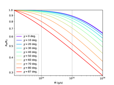
Figure 2: Magnetospheric radius in units of the corotation radius as a function of the mass accretion rate obtained for the case of an inclined rotator from Eq. 20. We assumed $P_{\rm spin}$=1.69 ms, $\alpha$=0.4, $\eta$=0.2, and $\gamma$=1.0. Different values for the inclination angle are shown in different colors for clarity. The magnetic moment corresponding to each angle is obtained from Eq. 21 by assuming $\dot{P}_{\rm spin}$=5.39$\times$10^-21 s s^-1.

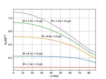
Figure 3: Comparison between the magnetospheric radius calculated according to the WG97 (see Eq. 20) and the GL79 (see Eq. 6) prescriptions as a function of the inclination angle and for five values of the mass accretion rates (including the highest considered value of the mass accretion rate and the minimum value for which solutions to Eq. 20 are found for all considered inclination angles). We assumed $P_{\rm spin}$=1.69 ms, $\alpha$=0.4, $\eta$=0.2, and $\gamma$=1.0. The magnetic moment corresponding to each angle is obtained from Eq. 21 by assuming $\dot{P}_{\rm spin}$=5.39$\times$10^-21 s s^-1 and $P_{\rm spin}$=1.69 ms.

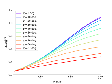
Figure 4: Similar to Fig. 3, but here the comparison between the two magnetospheric radius prescriptions is shown as a function of the mass accretion rate and for different inclination angles.

The interesting feature that emerges from Fig. 2 is that the magnetospheric radius gets progressively smaller when larger inclination angles are considered (at comparable mass accretion rates). For $\chi$$\gtrsim$60 deg, the magnetospheric radius can be up to a factor of $\sim$2.5 smaller than that of the aligned rotator case presented by W87 and W95. The direct comparison between the magnetospheric radius of an inclined dipole according to the WG97 theory and the GL79 treatment is shown in Fig. 3 and Fig. 4 (note that Eq. 6 has been calculated in both figures by using the case $\chi=0$ for the NS magnetic moment in Eq. 21, as the GL79 approach is formally derived in case of an orthogonal rotator). Figure 3 shows the ratio between the magnetospheric radius of W97 and GL79 as a function of the inclination angle for three values of the mass accretion rate. This is similar to Fig. 2 in WG97 but we made use of a full (and not simplified) solution to Eq. 20 and use $R_{\rm M}^{\rm GL79}$ instead of $R_{\rm A}$ in the comparison. Figure 4 shows the ratio between the magnetospheric radius of W97 and GL79 as a function of the mass accretion rate for different inclination angles, highlighting the fact that the largest difference between the magnetospheric radius in the two treatments occurs toward lower mass accretion rates and higher inclination angles (with the effect of the inclination angle being more effective toward higher mass accretion rates).

3 Application to low level accretion onto transitional millisecond pulsars

Transitional millisecond pulsars are a sub-class of low mass X-ray binaries (LMXBs) hosting a NS which have been observed to switch between the rotation-powered to accretion-powered regimes (see, e.g. Kluzniak et al., 1988; Tauris, 2015). So far, 3 confirmed systems have been identified: PSR J1023+0038 (Archibald et al., 2009; Patruno et al., 2014), XSS J12270-4859 (Saitou et al., 2009; de Martino et al., 2010, 2014), and IGR J18245-2452 (Papitto et al., 2013; Ferrigno et al., 2014). The pulse period of the first two systems is strikingly similar, $\sim$1.69 ms. IGR J18245-2452 hosts a NS spinning at 3.9 ms. Two candidate systems, 3FGL J1544.6-1125 and 3FGL J0427.9-6704, have been suggested by Bogdanov & Halpern (2015) and Strader et al. (2016), but no spin period has yet been reported for these sources. In the rotation-powered regime, the pressure of the NS dipole radiation is believed to push away the surrounding accretion disk and the compact object shines as a millisecond radio pulsar. In this state, only a moderate X-ray luminosity of $\lesssim$10³² erg s^-1 is recorded. This is ascribed to the presence of an intra-binary shock formed by the interaction between the pulsar wind and the material lost by the companion star (see, e.g., Bogdanov et al., 2014; Bassa et al., 2014). When the accretion disk is formed around the NS, the system switches to an accretion powered regime. So far, only IGR J18245-2452 displayed an accretion powered X-ray regime with a peak luminosity (10³⁶-10³⁷ erg s^-1) and spectral/timing properties similar to those of classical accreting millisecond X-ray pulsars in outburst (hereafter, AMXPs; Patruno & Watts, 2012). The two other confirmed systems and the candidate transitional pulsar likely underwent only some lower level accretion episodes, with typical luminosities of a few 10³³ erg s^-1. This “sub-luminous disk state” (Linares, 2014; Papitto et al., 2015) is usually characterized by a prominent variability in X-rays, and the presence of three distinct emission modes: a low mode, during which the luminosity can be as low as $\sim$5$\times$10³² erg $s^{-1}$, a high mode in which the typical luminosity is $\sim$(3-5)$\times$10³³ erg $s^{-1}$, and a flaring mode where the luminosity can increase by another factor of $\sim$10. The switch between the different modes can be as fast as a few seconds, and the mechanism regulating these switches has not yet been understood (Bogdanov et al., 2014). During the high mode, the X-ray emission of transitional pulsars displays little variability and this is the only mode where X-ray pulsations could be clearly identified from both XSS J12270-4859 and PSR J1023+0038. For the first source, Papitto et al. (2015) measured a high mode average X-ray luminosity of $L_{\rm X}$$\sim$5$\times$10³³ erg s^-1 (assuming a source distance of 1.40 kpc) and a pulsed fraction of 6-7% in the 0.5-11 keV energy range. For PSR J1023+0038, Archibald et al. (2015) measured an average high mode luminosity of $L_{\rm X}$$\sim$3$\times$10³³ erg s^-1 (0.3-10 keV) and a pulsed fraction of about 8% in a similar energy band (for a source distance of 1.37 kpc). In both cases, the authors interpreted the observed X-ray pulsations as due to accretion onto the NS (see also Ambrosino et al., 2017, who found indications for a rotationally-powered activity from PSR J1023+0038).

Although the phenomenologically complex sub-luminous disk state of the transitional pulsars is still lacking an exhaustive interpretation and many questions remain open (Campana et al., 2016), the discovery of accretion powered X-ray pulsations at the low X-ray luminosities of the high mode is particularly puzzling because it challenges the “standard” accretion scenario that is usually invoked to interpret the observations of transitional pulsars and other classes of accreting millisecond NS X-ray binaries (see below). In the following, we focus on this peculiar property of the high emission mode and in particular on the consideration of how low level accretion in these sources could still give rise to X-ray pulsations at such unprecedentedly low X-ray luminosity level. Our considerations are presently unable to explain also other phenomena observed in the sub-luminous disk state. We plan to discuss these in a future extension of this work.

It is generally believed that accretion in a disk-fed NS LMXB can only take place as long as the NS magnetospheric radius is smaller than the corotation radius (see, e.g., Frank et al., 2002). According to this standard scenario, when $R_{\rm M}$ becomes larger than $R_{\rm c}$, it is expected that the centrifugal force at the boundary between the NS magnetosphere and material in the disk pushes the inflowing matter away, inhibiting accretion and driving outflows (the so-called “propeller effect”; Illarionov & Sunyaev, 1975). To estimate the X-ray luminosity at which the onset of the propeller is expected in the case of the transitional pulsars, Papitto et al. (2015) and Archibald et al. (2015) used an expression for the magnetospheric radius very similar to the GL79 prescription (see Eq. 6). As a result of this calculation they found that in both XSS J12270-4859 and PSR J1023+0038 accretion should be strongly inhibited already at luminosities $L_{\rm X}$$\gtrsim$2$\times$10³⁵ erg s^-1. These authors thus suggested that the detection of X-ray pulsations in the sub-luminous disk state of these systems should not occur, unless very powerful outflows are generated by the rotating NS magnetosphere which remove $\gtrsim$95-99% of the matter inflowing at the inner disk boundary. If this were the case, the large mass inflow rate would maintain $R_{\rm M}$$<$$R_{\rm c}$, such that low level accretion could take place in the standard scenario.

While the presence of outflows in transitional pulsars has been supported by radio observations (see, e.g., Hill et al., 2011; Ferrigno et al., 2014), a quantitative estimate of the ratio between the inflowing and outflowing mass rate from these systems cannot be reliably constrained yet from the observations. Advanced magnetohydrodynamic simulations of a rapidly rotating NS surrounded by a disk show that outflows can be generated in the so-called “weak propeller regime”, when $R_{\rm M}$$\gtrsim$$R_{\rm c}$, but the mass ejection rate is at the most comparable to the mass accretion rate (not larger than $\sim$20% of the total mass inflow rate in the simulations of Ustyugova et al., 2006). In the strong propeller regime, when $R_{\rm M}$$\gg$$R_{\rm c}$, the ejection efficiency can reach about 80% (Lii et al., 2014; Lovelace et al., 2013) that is still significantly lower than the level required in the cases of XSS J12270-4859 and PSR J1023+0038. In the strong propeller regime it is also unlikely that the bulk of the X-ray emission is dominated by residual accretion. As an example, in the case of IGR J18245-2452, the strong propeller regime has been invoked to explain the dramatic hardening of the source X-ray emission in terms of shocks that form between the outflows and the surrounding medium (rather than by residual accretion; see, e.g., Ferrigno et al., 2014).

Only in the white dwarf binary AE Aquarii, evidence has been found for propelling efficiencies as high as 97% (Oruru & Meintjes, 2012). Therefore, it has been suggested that such extreme values cannot be ruled out. We show below that the need of extreme ejection efficiencies to explain the X-ray pulsations of transitional pulsars in the sub-luminous disk state might not be needed if the WG97 prescription of the magnetospheric radius is used in place of the GL79 simplified model.

The luminosities at which pulsations have been detected in the X-ray emission of XSS J12270-4859 and PSR J1023+0038 correspond to mass accretion rates of $\dot{M}$$\approx$$L_{\rm X}$$R_{\rm NS}$/(G$M_{\rm NS}$)=(2-3)$\times$10¹³ g s^-1. The approximate model of GL79 would give a magnetospheric radius at these very low mass accretion rates that is $\sim$3 times larger than the corotation radius, thus requiring the extreme outflows invoked by Papitto et al. (2015) and Archibald et al. (2015) to allow for (at least) some residual accretion and X-ray pulsations. According to WG97 calculations, the magnetospheric radius is still significantly smaller than the corotation radius even at mass accretion rates as low as $\sim$2-3$\times$10¹³ g s^-1. In case the NS is endowed with a large inclination angle ($\chi$$\gtrsim$60-70 deg), the magnetospheric radius is further reduced compared to the GL79 approach (even though this parameter is more effective at reducing the magnetospheric radius toward higher mass accretion rates; see Fig. 2). Under these assumptions, little to no outflows would thus be required to explain the pulsations at the very low X-ray luminosities recorded from XSS J12270-4859 and PSR J1023+0038 in the high mode of the sub-luminous-disk state.

For all computations in Fig. 2 we have assumed that the inclination angle also determines the effective dipole magnetic moment of the NS estimated through Eq. 21 and a spin period derivative of 5.39$\times$10^-21 s s^-1, as observationally measured in the case of PSR J1023+0038 (Archibald et al., 2013). These results are thus equally applicable to the case of XSS J12270-4859, as the spin period of the NS hosted in this system is virtually identical to that of PSR J1023+0038 and also the spin period derivatives of the two systems are fairly similar (Roy et al., 2015).

Interestingly, some evidence for a large inclination angle ($>$60 deg) between the rotation and magnetic axis of the NS in XSS J12270-4859 was provided by Papitto et al. (2015), using also the results published by de Martino et al. (2014). This makes our application of the W97 prescription for the magnetospheric radius calculation at large inclination angles promising for transitional millisecond pulsars in general.

4 Discussion and conclusions

In this paper we reviewed the basic assumptions of the magnetically threaded disk model for accreting NS in X-ray binaries in both the original treatment presented by GL79 and the revised approach by W87 and WG95. The models make different predictions for the magnetospheric radius as a function of the mass accretion rate, with WG97 also extending the calculations to the case of an inclined dipole. The simplified approach of GL79 predicts that the magnetospheric radius is proportional to $\dot{M}^{-2/7}$. In the approach of W87 and W95 for an aligned rotator, the increase of the magnetospheric radius for decreasing mass accretion rates is slower and more complex. The most noticeable difference between these approaches occur at lower mass accretion rates. Moreover, when the full equations given in WG97 are solved, the magnetospheric radius is found to be further reduced at large inclination angles between the NS rotation and magnetic axes (with an effect more pronounced toward larger mass accretion rates). Assuming for consistency in all cases the same value of the screening parameter $\eta$=0.2, the magnetospheric radius obtained from WG97 can be as small as $\sim$0.3 times the value expected from the GL79 calculations either for low mass accretion rates ($\sim$10¹³-10¹⁵ g s^-1) or for higher mass accretion rates ($\gtrsim$10¹⁵ g s^-1) and large inclination angles ($\chi\gtrsim 60$ deg).

We applied the magnetospheric radius prescription of W97 to the case of transitional millisecond pulsars, which are a sub-class of NS LMXBs showing a peculiar X-ray variability during their so-called sub-luminosity accretion state. The phenomenology observed during this state is complex, with three different emission modes identified (high, low, flaring) and rapid switches (a few seconds) occurring between them. So far there is still not an agreed scenario to explain all these behaviors, and we focused here in particular on the puzzling accretion-driven X-ray pulsations observed only during the high mode at an unprecedentedly low luminosity level (2-3$\times$10³³ erg s^-1) compared to that of other previously known accreting millisecond X-ray pulsars in LMXBs ($\gtrsim$10³⁵ erg s^-1). Following the usually adopted GL79 approach for the calculation of the magnetospheric radius, it is expected that at the mass accretion rates corresponding to a luminosity of 2-3$\times$10³³ erg s^-1, the system should enter a very strong propeller regime with virtually no accretion taking place (and thus no detectable X-ray pulsations). Other works in the literature about the high mode of the transitional pulsars have proposed a scenario in which there is a substantial mass transfer from the companion to the NS to sufficiently compress the compact object magnetosphere and formally allow accretion, but at least $\sim$95-99% of this material is ejected away by a very efficient propeller to explain the low luminosity at which pulsations are recorded (Papitto et al., 2015; Archibald et al., 2015). Even though these high propelling efficiencies can not be completely ruled out from the analogy with the white dwarf binary AE Aquarii, they are difficult to be reconciled with currently available MHD simulations of accreting NS in LMXBs. We showed that the revised magnetically threaded disk model presented by WG97 predicts a substantially smaller magnetospheric disk radius compared to GL79, especially when low mass accretion rates and high inclination angles between the NS magnetic and rotational axis are considered (assuming consistent values of the other involved parameters). If WG97 approach is used to estimate the magnetospheric radius, it is possible to envisage that accretion still takes place in the transitional pulsars when the mass accretion rate from the companion is as low as (2-3)$\times$10^-13 g s^-1. This could potentially explain how to produce accretion-driven X-ray pulsations at a luminosity of 2-3$\times$10³³ erg s^-1 without invoking very strong propellers.

Appendix A Full derivation of Eq. 20

We report here for reference the detailed calculations to derive Eq. 20. Following W97 approach, let us consider a NS endowed with a tilted dipolar magnetic field:

$$B_{R} =2\eta\Bigl{(}\frac{\mu}{R^{3}}\Bigr{)}\sin\chi\cos\phi$$ (22)

$$B_{\phi} =\eta\Bigl{(}\frac{\mu}{R^{3}}\Bigr{)}\sin\chi\sin\phi+b_{\phi}$$

$$B_{z} =\eta\Bigl{(}\frac{\mu}{R^{3}}\Bigr{)}\cos\chi.$$

Here, $\chi$ is the tilt angle between the NS magnetic and rotational axes, while $b_{\phi}$ is the magnetic field generated by the interaction of the NS magnetic field lines with the disk material in a Keplerian orbit around the compact object. This field is expressed at the upper ($z=h$) and inner ($R=R_{\rm 0}$) surface of the disk as follows:

$$b^{(\rm upper)}_{\phi} =-\Gamma\Bigl{[}1-\Bigl{(}\frac{\Omega_{\rm NS}}{\Omega_{\rm K}}\Bigr{)}\Bigr{]}B_{z}$$ (23)

$$b^{(\rm inner)}_{\phi} =\Gamma\Bigl{[}1-\Bigl{(}\frac{\Omega_{\rm NS}}{\Omega_{\rm K}}\Bigr{)}\Bigr{]}B_{R}$$

Due to the symmetry of the problem $b_{\phi}(z)=-b_{\phi}(-z)$. We derive first Eq. 19 by starting from the Euler equation in a stationary state:

$$\rho(\@vec{v}\cdot\nabla)\@vec{v}=-\nabla P-\rho\nabla\Phi+\frac{1}{4\pi}\bigl{(}\nabla\times\@vec{B}\bigr{)}\times\@vec{B}$$ (24)

According to Eq. A, $B_{z}$ does not depend on $\phi$, thus the azimuthal component of the Lorentz force can be written as:

$$\frac{1}{4\pi}\bigl{[}\bigl{(}\nabla\times\@vec{B}\bigr{)}\times\@vec{B}\bigr{]}_{\phi}=\frac{1}{4\pi}\Bigl{[}\frac{1}{R}B_{\phi}B_{R}+B_{R}\partial_{R}(B_{\phi})+B_{z}\partial_{z}(B_{\phi})-\frac{1}{R}B_{R}\partial_{\phi}(B_{R})\Bigr{]}$$

Using the identity

$$\bigl{(}\@vec{v}\cdot\nabla\bigr{)}\@vec{v}=\frac{1}{2}\nabla v^{2}+\bigl{(}\nabla\times\@vec{v}\bigr{)}\times\@vec{v}$$

we can rewrite the $\phi$ component of the left hand side of Eq. 24 as:

$$\begin{split}&\rho\bigl{[}\frac{1}{2}\nabla v^{2}+\bigl{(}\nabla\times\@vec{v}\bigr{)}\times\@vec{v}\bigr{]}_{\phi}=\rho\Bigl{[}\frac{1}{2R}\partial_{\phi}(v^{2})+\frac{1}{R}v_{\phi}v_{R}+v_{R}\partial_{R}(v_{\phi})+\\ &+v_{z}\partial_{z}(v_{z})-\frac{1}{R}v_{r}\partial_{\phi}(v_{r})-\frac{1}{R}v_{z}\partial_{\phi}(v_{z})\Bigr{]}=\\ &=\frac{\rho}{R}v_{R}\partial_{R}(Rv_{\phi})+\frac{\rho}{2R}\partial_{\phi}(v_{\phi}^{2}).\end{split}$$

Here we also assumed that the matter leaves the disk only once inside the magnetospheric radius and that for a thin disk $v_{\rm z}=0$. We thus obtain:

$$\begin{split}&\rho Rv_{R}\partial_{R}(Rv_{\phi})=\\ &\frac{1}{4\pi}\Bigl{[}B_{\phi}B_{R}R+R^{2}B_{R}\partial_{R}(B_{\phi})+R^{2}B_{z}\partial_{z}(B_{\phi})-RB_{R}\partial_{\phi}(B_{R})\Bigr{]}+\\ &-\rho R\partial_{\phi}\Phi-R\partial_{\phi}(P)-\frac{\rho}{2}R\partial_{\phi}(v^{2}_{\phi})\end{split}$$ (25)

Here the term $\partial_{\phi}\Phi$ vanishes due to the axial symmetry of gravitational potential. Under the further assumption that $P$ and $v_{\phi}$ are $\phi$-independent with $v_{\phi}\simeq\Omega_{K}R$, we can write:

$$\begin{split}&\rho Rv_{R}\partial_{R}(\Omega_{\rm K}R^{2})=\\ &\frac{1}{4\pi}\Bigl{[}B_{\phi}B_{R}R+R^{2}B_{R}\partial_{R}(B_{\phi})+R^{2}B_{z}\partial_{z}(B_{\phi})-RB_{R}\partial_{\phi}(B_{R})\Bigr{]}\end{split}$$ (26)

Equation 26 can be written in the following way:

$$\rho Rv_{R}\partial_{R}(\Omega_{\rm K}R^{2})=\frac{1}{4\pi}\Bigl{[}\partial_{R}(R^{2}b_{\phi}B_{R})+\partial_{z}(b_{\phi}B_{z})R^{2}\Bigr{]}+A(R,\phi,z)$$ (27)

where

$$\int^{2\pi}_{0}A(R,\phi,z)d\phi=0.$$ (28)

To demonstrate Eq. 27, note that:

$$R^{2}B_{R}\partial_{R}B_{\phi}=\partial(R^{2}B_{R}B_{\phi})-2RB_{\phi}B_{R}-R^{2}B_{\phi}\partial_{R}B_{R},$$

and

$$R^{2}B_{z}\partial_{z}B_{\phi}=R^{2}\partial_{z}(B_{z}B_{\phi})-R^{2}B_{\phi}\partial_{z}B_{z}.$$

We thus obtain for the right hand side of Eq. 26

$$\begin{split}&=\frac{1}{4\pi}\bigl{\{}\partial_{R}(R^{2}B_{R}B_{\phi})+R^{2}\partial_{z}(B_{z}B_{\phi})-R^{2}B_{\phi}\bigl{[}\partial_{R}(B_{R})+\partial_{z}(B_{z})\bigr{]}+\\ &-RB_{R}\partial_{\phi}(B_{R})-RB_{\phi}B_{R}\bigr{\}}\end{split}$$

From the second Maxwell equation, we have:

$$\partial_{R}(B_{R})+\partial_{z}(B_{z})=-\frac{B_{R}}{R}-\frac{1}{R}\partial_{\phi}B_{\phi},$$

and thus:

$$\begin{split}&\frac{1}{4\pi}\bigl{[}\partial_{R}(R^{2}B_{R}B_{\phi})+R^{2}\partial_{z}(B_{\phi}B_{z})+R^{2}B_{\phi}\bigl{(}\frac{B_{R}}{R}+\frac{1}{R}\partial_{\phi}(B_{\phi})\bigr{)}\\ &-RB_{R}\partial_{\phi}(B_{R})-RB_{\phi}B_{z}\bigr{]}=\\ &=\frac{1}{4\pi}\bigl{[}\underbrace{\partial_{R}(R^{2}B_{R}B_{\phi})}_{i}+\underbrace{R^{2}\partial_{z}(B_{\phi}B_{z})}_{ii}+\underbrace{RB_{\phi}\partial_{\phi}(B_{\phi})}_{iii}-\underbrace{RB_{R}\partial_{\phi}(B_{R})}_{iv}\bigr{]}\end{split}$$

By using the relation

$$B_{\phi}=b_{\phi}-\frac{1}{2}\partial_{\phi}(B_{R})$$ (29)

that can be obtained from Eq. A, we can rewrite the four terms above as:

$$\begin{split}&i\rightarrow\partial_{R}(R^{2}B_{R}B_{\phi})=\partial_{R}(R^{2}b_{\phi}B_{R})-\frac{1}{2}\partial_{R}[R^{2}B_{R}\partial_{\phi}(B_{R})]\\ &ii\rightarrow R^{2}\partial_{z}(B_{\phi}B_{z})=R^{2}\partial_{z}(b_{\phi}B_{z})-\frac{R^{2}}{2}\partial_{z}[B_{z}\partial_{\phi}(B_{R})]\\ &iii\rightarrow RB_{\phi}\partial_{\phi}(B_{\phi})=\frac{1}{2}R\partial_{\phi}(B^{2}_{\phi})\\ &iv\rightarrow-RB_{R}\partial_{\phi}(B_{R})=-\frac{1}{2}R\partial_{\phi}(B^{2}_{R}),\\ \end{split}$$

and thus:

$$\begin{split}&A(R,\phi,z)=\\ &-\frac{1}{8\pi}\Bigl{\{}\underbrace{\partial_{R}\bigl{[}R^{2}B_{R}\partial_{\phi}(B_{R})\bigr{]}}_{\alpha}+\underbrace{R^{2}\partial_{z}\bigl{[}B_{z}\partial_{\phi}(B_{R})\bigr{]}}_{\beta}+\underbrace{R\partial_{\phi}(B^{2}_{R}-B^{2}_{\phi})}_{\gamma}\Bigr{\}}\\ \end{split}$$

To prove Eq. 28, it is sufficient to note that $B_{z}$ does not depend on $\phi$ and that for a generic function $f(R,\phi,z)$:

$$\int^{2\pi}_{0}\partial_{\phi}(f)d\phi=f(2\pi)-f(0)=0$$ (30)

Equation 27 has now to be integrated over $\phi$ from $0$ to $2\pi$ and over $z$ from $-h$ to $h$. Taking into account the simplifications possible under the assumption of a thin disk case and the continuity equation:

$$\dot{M}=-\int^{2\pi}_{0}Rd\phi\int^{h}_{-h}\rho v_{R}dz,$$

we obtain for the left hand side of Eq. 27:

$$\begin{split}&\int^{2\pi}_{0}d\phi\int^{h}_{-h}dz\rho Rv_{R}\partial_{R}(\Omega_{\rm K}R^{2})=\frac{d}{dR}(\Omega_{\rm K}R^{2})R\int^{2\pi}_{0}d\phi\int^{h}_{-h}dz\rho v_{R}=\\ &=-\dot{M}\frac{d}{dR}(\Omega_{\rm K}R^{2})\end{split}$$

For the first and second right hand side term of Eq. 27, we have:

$$\begin{split}&\int^{2\pi}_{0}d\phi\int^{h}_{-h}dz\partial_{R}\Bigl{(}R^{2}\frac{b_{\phi}B_{R}}{4\pi}\Bigr{)}=\frac{1}{4\pi}\int^{2\pi}_{0}d\phi\partial_{R}\Bigl{(}R^{2}\int^{h}_{-h}b_{\phi}B_{R}dz\Bigr{)}=\\ &=\frac{h}{2\pi}\frac{d}{dR}\Bigl{(}R^{2}\int^{2\pi}_{0}b^{(\rm inner)}_{\phi}B_{R}d\phi\Bigr{)}=h\frac{d}{dR}\bigl{(}R^{2}\langle b^{(\rm inner)}_{\phi}B_{R}\rangle\bigr{)}\end{split}$$

and

$$\int^{2\phi}_{0}d\phi\int^{h}_{-h}dzR^{2}\partial_{z}\Bigl{(}\frac{b_{\phi}B_{z}}{4\pi}\Bigr{)}=\frac{R^{2}}{4\pi}\int^{2\pi}_{0}d\phi\bigl{[}b_{\phi}B_{z}\bigr{]}^{h}_{-h}=R^{2}b^{(\rm upper)}_{\phi}B_{z},$$

respectively. Putting all terms together, we get at $R$=$R_{\rm M}$:

$$\dot{M}\frac{d}{dR}\bigl{(}\Omega_{\rm K}r^{2}\bigr{)}=\underbrace{-h\frac{d}{dR}\bigl{(}R^{2}\langle b^{(\rm inner)}_{\phi}B_{R}\rangle\bigr{)}}_{I}-\underbrace{b^{(\rm upper)}_{\phi}B_{z}R^{2}}_{II}$$

For the left hand side, we have:

$$\dot{M}\frac{d}{dR}\bigl{(}\Omega_{\rm K}r^{2}\bigr{)}_{R_{\rm M}}=\dot{M}\frac{d}{dR}\bigl{(}\sqrt{GMR}\bigr{)}_{R_{\rm M}}=\frac{\dot{M}GM}{2\sqrt{R_{\rm M}}}$$

For the two terms on the right hand side, we have:

$$\begin{split}I\rightarrow&-h\frac{d}{dR}(R^{2}\langle b^{(\rm inner)}_{\phi}B_{R}\rangle)=\\ &-\frac{h\Gamma}{2\pi}\frac{d}{dR}\Bigl{\{}R^{2}\Bigl{[}1-\Bigl{(}\frac{\Omega_{\rm NS}}{\Omega_{\rm K}}\Bigr{)}\Bigr{]}\int^{2\pi}_{0}B^{2}_{R}d\phi\Bigr{\}}=\\ &=\frac{h\Gamma\eta^{2}\mu^{2}}{R^{5}}\sin^{2}\chi\Bigl{[}8-5\Bigl{(}\frac{\Omega_{\rm NS}}{\Omega_{\rm K}}\Bigr{)}\Bigr{]}\rightarrow\frac{h_{0}\Gamma\eta^{2}\mu^{2}}{R^{5}_{0}}\sin^{2}\chi(8-5\omega)\end{split}$$

and

$$\begin{split}II\rightarrow&-b^{(\rm upper)}_{\phi}B_{z}R^{2}=\Gamma R^{2}\Bigl{[}1-\Bigl{(}\frac{\Omega_{\rm NS}}{\Omega_{\rm K}}\Bigr{)}\Bigr{]}B^{2}_{z}=\\ &\rightarrow\frac{\Gamma\eta^{2}\mu^{2}}{R^{4}}\cos^{2}\chi(1-\omega).\end{split}$$

We finally get:

$$\dot{M}\sqrt{GMR_{\rm M}}=\frac{2\Gamma\eta^{2}\mu^{2}}{R^{3}_{0}}\Bigl{[}(1-\omega)\cos^{2}\chi+\Bigl{(}\frac{h_{0}}{R_{\rm M}}\Bigr{)}(8-5\omega)\sin^{2}\chi\Bigr{]}.$$

References

- Alpar & Shaham (1985) Alpar, M. A. & Shaham, J. 1985, Nature, 316, 239
- Ambrosino et al. (2017) Ambrosino, F., Papitto, A., Stella, L., et al. 2017, ArXiv e-prints
- Archibald et al. (2015) Archibald, A. M., Bogdanov, S., Patruno, A., et al. 2015, ApJ, 807, 62
- Archibald et al. (2013) Archibald, A. M., Kaspi, V. M., Hessels, J. W. T., et al. 2013, ArXiv e-prints
- Archibald et al. (2009) Archibald, A. M., Stairs, I. H., Ransom, S. M., et al. 2009, Science, 324, 1411
- Bassa et al. (2014) Bassa, C. G., Patruno, A., Hessels, J. W. T., et al. 2014, MNRAS, 441, 1825
- Bhattacharya & van den Heuvel (1991) Bhattacharya, D. & van den Heuvel, E. P. J. 1991, Phys. Rep, 203, 1
- Bogdanov et al. (2014) Bogdanov, S., Archibald, A. M., Bassa, C., et al. 2014, ArXiv e-prints
- Bogdanov & Halpern (2015) Bogdanov, S. & Halpern, J. P. 2015, ApJ, 803, L27
- Bozzo et al. (2008) Bozzo, E., Falanga, M., & Stella, L. 2008, ApJ, 683, 1031
- Bozzo et al. (2009) Bozzo, E., Stella, L., Vietri, M., & Ghosh, P. 2009, A&A, 493, 809
- Campana et al. (2016) Campana, S., Coti Zelati, F., Papitto, A., et al. 2016, A&A, 594, A31
- D’Angelo & Spruit (2010) D’Angelo, C. R. & Spruit, H. C. 2010, MNRAS, 406, 1208
- de Martino et al. (2014) de Martino, D., Casares, J., Mason, E., et al. 2014, MNRAS, 444, 3004
- de Martino et al. (2010) de Martino, D., Falanga, M., Bonnet-Bidaud, J.-M., et al. 2010, A&A, 515, A25
- Erkut & Alpar (2004) Erkut, M. H. & Alpar, M. A. 2004, ApJ, 617, 461
- Ferrigno et al. (2014) Ferrigno, C., Bozzo, E., Papitto, A., et al. 2014, A&A, 567, A77
- Frank et al. (2002) Frank, J., King, A., & Raine, D. J. 2002, Accretion Power in Astrophysics: Third Edition
- Ghosh (2007) Ghosh, P. 2007, Rotation And Accretion Powered Pulsars. Series: World Scientific Series in Astronomy and Astrophysics, ISBN: ¡ISBN¿978-981-02-4744-7¡/ISBN¿. WORLD SCIENTIFIC, Edited by Pranab Ghosh, vol. 10, 10
- Ghosh & Lamb (1979) Ghosh, P. & Lamb, F. K. 1979, ApJ, 232, 259
- Hill et al. (2011) Hill, A. B., Szostek, A., Corbel, S., et al. 2011, MNRAS, 415, 235
- Illarionov & Sunyaev (1975) Illarionov, A. F. & Sunyaev, R. A. 1975, A&A, 39, 185
- Jetzer et al. (1998) Jetzer, P., Strässle, M., & Straumann, N. 1998, New A, 3, 619
- King (2012) King, A. 2012, Mem. Soc. Astron. Italiana, 83, 466
- King et al. (2013) King, A. R., Livio, M., Lubow, S. H., & Pringle, J. E. 2013, MNRAS, 431, 2655
- Kluźniak & Rappaport (2007) Kluźniak, W. & Rappaport, S. 2007, ApJ, 671, 1990
- Kluzniak et al. (1988) Kluzniak, W., Ruderman, M., Shaham, J., & Tavani, M. 1988, Nature, 334, 225
- Lai (1999) Lai, D. 1999, ApJ, 524, 1030
- Lai (2014) Lai, D. 2014, in European Physical Journal Web of Conferences, Vol. 64, European Physical Journal Web of Conferences, 1001
- Lamb et al. (1985) Lamb, F. K., Shibazaki, N., Alpar, M. A., & Shaham, J. 1985, Nature, 317, 681
- Lii et al. (2014) Lii, P. S., Romanova, M. M., Ustyugova, G. V., Koldoba, A. V., & Lovelace, R. V. E. 2014, MNRAS, 441, 86
- Linares (2014) Linares, M. 2014, ApJ, 795, 72
- Lovelace et al. (2013) Lovelace, R. V. E., Romanova, M. M., & Lii, P. 2013, ArXiv e-prints
- Muñoz-Darias et al. (2014) Muñoz-Darias, T., Fender, R. P., Motta, S. E., & Belloni, T. M. 2014, MNRAS, 443, 3270
- Oruru & Meintjes (2012) Oruru, B. & Meintjes, P. J. 2012, MNRAS, 421, 1557
- Papitto et al. (2015) Papitto, A., de Martino, D., Belloni, T. M., et al. 2015, MNRAS, 449, L26
- Papitto et al. (2013) Papitto, A., Ferrigno, C., Bozzo, E., et al. 2013, Nature, 501, 517
- Parfrey et al. (2017) Parfrey, K., Spitkovsky, A., & Beloborodov, A. M. 2017, MNRAS, 469, 3656
- Parfrey & Tchekhovskoy (2017) Parfrey, K. & Tchekhovskoy, A. 2017, ArXiv e-prints
- Patruno et al. (2014) Patruno, A., Archibald, A. M., Hessels, J. W. T., et al. 2014, ApJ, 781, L3
- Patruno & Watts (2012) Patruno, A. & Watts, A. L. 2012, ArXiv e-prints
- Romanova et al. (2014) Romanova, M. M., Lovelace, R. V. E., Bachetti, M., et al. 2014, in European Physical Journal Web of Conferences, Vol. 64, European Physical Journal Web of Conferences, 5001
- Roy et al. (2015) Roy, J., Ray, P. S., Bhattacharyya, B., et al. 2015, ApJ, 800, L12
- Saitou et al. (2009) Saitou, K., Tsujimoto, M., Ebisawa, K., & Ishida, M. 2009, PASJ, 61, L13
- Shakura & Sunyaev (1973) Shakura, N. I. & Sunyaev, R. A. 1973, A&A, 24, 337
- Spitkovsky (2006) Spitkovsky, A. 2006, ApJ, 648, L51
- Strader et al. (2016) Strader, J., Li, K.-L., Chomiuk, L., et al. 2016, ApJ, 831, 89
- Tauris (2015) Tauris, T. M. 2015, ArXiv e-prints
- Ustyugova et al. (2006) Ustyugova, G. V., Koldoba, A. V., Romanova, M. M., & Lovelace, R. V. E. 2006, ApJ, 646, 304
- Walter et al. (2015) Walter, R., Lutovinov, A. A., Bozzo, E., & Tsygankov, S. S. 2015, A&A Rev., 23, 2
- Wang (1987) Wang, Y.-M. 1987, A&A, 183, 257
- Wang (1995) Wang, Y.-M. 1995, ApJ, 449, L153
- Wang (1997) Wang, Y.-M. 1997, ApJ, 475, L135