Generalised Born-Infeld models, Lax operators and the $\textsc{T}\bar{\textsc{T}}$ perturbation

Abstract

Surprising links between the deformation of 2D quantum field theories induced by the composite $\textsc{T}\bar{\textsc{T}}$ operator, effective string models and the $AdS/$CFT correspondence, have recently emerged. The purpose of this article is to discuss various classical aspects related to the deformation of 2D interacting field theories. Special attention is given to the sin(h)-Gordon model, for which we were able to construct the $\textsc{T}\bar{\textsc{T}}$-deformed Lax pair. We consider the Lax pair formulation to be the first essential step toward a more satisfactory geometrical interpretation of this deformation within the integrable model framework.

Furthermore, it is shown that the 4D Maxwell-Born-Infeld theory, possibly with the addition of a mass term or a derivative-independent potential, corresponds to a natural extension of the 2D examples. Finally, we briefly comment on 2D Yang-Mills theory and propose a modification of the heat kernel, for a generic surface with genus $p$ and $n$ boundaries, which fully accounts for the $\textsc{T}\bar{\textsc{T}}$ contribution.

1 Introduction

Effective Field Theories (EFTs), are characterized by the presence of irrelevant fields in the Lagrangian which usually make quantization and the physical interpretation of the high-energy regime very problematic. In two spacetime dimensions, the study of EFTs is experiencing a period of renewed interest thanks to the discovery of surprising integrable-like properties of the $\textsc{T}\bar{\textsc{T}}$ composite operator, rigorously defined by Zamolodchikov Zamolodchikov:2004ce as the determinant of the stress-energy tensor.

While the main source of inspiration of Zamolodchikov:2004ce were the non-perturbative factorization properties detected, within the Form-Factor approach, in Fateev:1997yg , the $\textsc{T}\bar{\textsc{T}}$ perturbative contributions to the finite-size spectrum first emerged from the study of the RG flow connecting the Tricritical Ising (TIM) to the Ising model (IM) Zamolodchikov:1991vx . The analysis of Zamolodchikov:1991vx , was based on a combination of powerful techniques such as conformal perturbation theory, exact scattering theory and the Thermodynamic Bethe Ansatz (TBA).

The scattering among right and left mover massless excitations along the TIM $\rightarrow$ IM critical line is described by a pure CDD Castillejo:1955ed factor which, therefore, should contain information on irrelevant fields. This observation triggered early studies on TBA models with modified CDD kernels and lead to the conclusion that, in many cases, they were affected by short-distance instabilities Alzam ; Mussardo:1999aj (see the related discussion in Section 9 of Smirnov:2016lqw ). The fact that seemingly consistent exact S-matrix models may display ultraviolet pathological behavior was first detected in Ravanini:1992fi . The interest towards this research topic remained very limited for many years until an important step forward was made in dubovsky2012solving ; dubovsky2012effective : a link between the TBA equations for free massless bosons, modified by a specific CDD factor, and the spectrum of effective bosonic closed strings was discovered. The generalization to open strings, to other conformal field theories and the observation that the effective action describing the confining flux tube of a generic gauge theory was described, at least at leading order, by a $\textsc{T}\bar{\textsc{T}}$ perturbation was made in Caselle:2013dra . The connection between these observations and the paper Zamolodchikov:2004ce was further clarified in Smirnov:2016lqw ; Cavaglia:2016oda where, among many other results, an inviscid Burgers equation for the spectrum was identified, and the corresponding equation for the action Smirnov:2016lqw lead to the reconstruction of the whole bosonic Born-Infeld (BI) Lagrangian in 2D Cavaglia:2016oda .

Triggered by these works, remarkable connections have emerged with the $AdS/$CFT duality McGough:2016lol ; Turiaci:2017zwd ; Giveon:2017nie ; Giveon:2017myj ; Asrat:2017tzd ; Giribet:2017imm ; Kraus:2018xrn ; Cottrell:2018skz ; Baggio:2018gct ; Babaro:2018cmq and flat space Jackiw-Teitelboim (JT) gravity Dubovsky:2017cnj ; Dubovsky:2018bmo , together with generalizations to non Lorentz-invariant perturbations Bzowski:2018pcy ; Guica:2017lia ; Chakraborty:2018vja ; Apolo:2018qpq .

The study of partition functions of $\textsc{T}\bar{\textsc{T}}$-deformed models was started in Cavaglia:2016oda and further developed in Cardy:2018sdv ; Dubovsky:2018bmo ; Datta:2018thy . Interesting results on entanglement were recently obtained in Chakraborty:2018kpr ; Donnelly:2018bef . Finally, a link with stochastic processes was established and generalizations to higher spacetime dimensions proposed in Cardy:2018sdv (see also in Bonelli:2018kik ; Taylor:2018xcy ).

The purpose of this article is to further investigate the properties of $\textsc{T}\bar{\textsc{T}}$-deformed field theories. Firstly, we shall review some of the results reported in Cavaglia:2016oda , concerning classical bosonic Lagrangians with interacting potentials. We will prove that the fairly complicated expression for the perturbed Lagrangian, given in Cavaglia:2016oda , can be recast into a much simpler Born-Infeld type form. We shall also comment on the similarity between the inclusion of the potential term and a transformation property for the spectrum first spotted in Smirnov:2016lqw , as the coefficient of the bulk contribution of the unperturbed energy is modified. The latter results were anticipated in RTTalkIGST2017 and are partially connected, with some minor overlap, to the papers Baggio:2018gct ; Bonelli:2018kik . The $\textsc{T}\bar{\textsc{T}}$-deformed sine-Gordon model is also discussed in detail and the corresponding Lax operators are constructed.

Furthermore, motivated by the observations made many years ago in 1966JETP ; Barbashov:1967zzz which link plane wave scatterings in the 4D Maxwell-Born-Infeld (MBI) theory to a 2D bosonic Born-Infeld model, we shall show that the MBI Lagrangian satisfies a simple generalization of the equations described in Smirnov:2016lqw ; Cavaglia:2016oda , similar but different from the higher dimensional proposals of Cardy:2018sdv ; Bonelli:2018kik ; Taylor:2018xcy . The introduction of a mass term or a derivative independent potential in the original field theory affects the $\textsc{T}\bar{\textsc{T}}$-deformed Lagrangian as in the 2D examples.

Finally, we will briefly discuss the exactly solvable example of 2D Yang-Mills and conjecture a simple modification that includes the $\textsc{T}\bar{\textsc{T}}$ contribution in the partition functions, and more generally in the heat kernel for a generic surface with genus $p$ and $n$ boundaries.

2 Deformed interacting bosonic Lagrangians from the Burgers equation

In Smirnov:2016lqw ; Cavaglia:2016oda it was proven that the energy levels $E_{n}(R,\tau)$ associated to the stationary states $\ket{n}$ with spatial momenta $P_{n}(R)=\frac{2\pi k_{n}}{R}$, ($k_{n}\in\mathbb{Z}$), satisfy the following inhomogeneous Burgers equation

$$\partial_{\tau}E_{n}(R,\tau)=\frac{1}{2}\partial_{R}\left(E_{n}^{2}(R,\tau)-P_{n}^{2}(R)\right)=-\frac{R}{\pi^{2}}\braket{n}{\textsc{T}\bar{\textsc{T}}}{n}_{R}\;,$$ (1)

where the composite operator $\textsc{T}\bar{\textsc{T}}$ is defined up to total derivative terms as

$$\textsc{T}\bar{\textsc{T}}(z,\bar{z}):=\lim_{(z^{\prime},\bar{z}^{\prime})\rightarrow(z,\bar{z})}T(z,\bar{z})\bar{T}(z^{\prime},\bar{z}^{\prime})-\Theta(z,\bar{z})\Theta(z^{\prime},\bar{z}^{\prime})\;,$$ (2)

and the complex components $T$, $\bar{T}$ and $\Theta$ of the stress-energy tensor are related to the Euclidean components $T_{11}$, $T_{22}$ and $T_{12}$ by the following relations:

$$(x_{1},x_{2})=(x,t)\;,\;(z,\bar{z})=(x_{1}+\mathbbm{i}\,x_{2}\;,\;x_{1}-\mathbbm{i}\,x_{2})\;,$$ (3)

$$T_{11}=-\frac{1}{2\pi}(\bar{T}+T-2\Theta)\;,\;T_{22}=\frac{1}{2\pi}(\bar{T}+T+2\Theta)\;,\;T_{12}=T_{21}=\frac{\mathbbm{i}}{2\pi}(\bar{T}-T)\;.$$ (4)

At finite volume $R$, the expectation values of the Euclidean components of the stress-energy tensor are related to $E_{n}$ and $P_{n}$ through ZamolodchikovTBA :

$$E_{n}(R,\tau)=-R\bra{n}T_{22}\ket{n}\;,\;\partial_{R}E_{n}(R,\tau)=-\bra{n}T_{11}\ket{n}\;,\;P_{n}(R)=-\mathbbm{i}R\bra{n}T_{12}\ket{n}\;.$$ (5)

Since (1) holds for any $n$, in the following we will drop the subscript $n$: $E_{n}(R,\tau)=E(R,\tau)$ and $P_{n}(R)=P(R)=\frac{2\pi k}{R}\;,\;(k\in\mathbb{Z})$. As a side remark, notice that from Cavaglia:2016oda it follows

$$\left(\begin{array}[]{c}E(R,\tau)\\ P(R)\end{array}\right)=\left(\begin{array}[]{cc}\cosh{(\theta_{0})}&-\sinh{(\theta_{0})}\\ -\sinh{(\theta_{0})}&\cosh{(\theta_{0})}\end{array}\right)\left(\begin{array}[]{c}E(\mathcal{R}_{0},0)\\ P(\mathcal{R}_{0})\end{array}\right)\;,$$ (6)

with

$$\sinh{\theta_{0}}=\frac{\tau\,P(R)}{\mathcal{R}_{0}}=\frac{\tau\,P(\mathcal{R}_{0})}{R}\;,\;\cosh{\theta_{0}}=\frac{R+\tau\,E(R,\tau)}{\mathcal{R}_{0}}=\frac{\mathcal{R}_{0}+\tau\,E(\mathcal{R}_{0},0)}{R}\;,$$ (7)

and

$$\mathcal{R}_{0}^{2}=\left(R+\tau\,E(R,\tau)\right)^{2}-\tau^{2}P^{2}(R)\;,\;R^{2}=\left(\mathcal{R}_{0}+\tau\,E(\mathcal{R}_{0},0)\right)^{2}-\tau^{2}P^{2}(\mathcal{R}_{0})\;.$$ (8)

Therefore the solution to (1) can be written in implicit form as

$$E^{2}(R,\tau)-P^{2}(R)=E^{2}(\mathcal{R}_{0},0)-P^{2}(\mathcal{R}_{0},0)\;.$$ (9)

It would be interesting to check if there exists an extension to higher spacetime dimensions of the Lorentz-type map (6) corresponding to the generalizations of the $\textsc{T}\bar{\textsc{T}}$ deformation proposed in Cardy:2018sdv ; Bonelli:2018kik ; Taylor:2018xcy and/or to the quantum version of the Maxwell-Born-Infeld model discussed in Section 4.
If the boundary conditions at $\tau=0$ are the energy levels of a CFT, i.e. of the form:

$$E(R,0)=\frac{A}{R}\;,$$ (10)

the general solution to (1) is

$$E(R,\tau)=\frac{R}{2\tau}\left(-1+\sqrt{1+\frac{4\tau}{R^{2}}A+\frac{4\tau^{2}}{R^{2}}P^{2}(R)}\right)=\frac{R}{2\tau}\left(-1+\sqrt{1+\frac{4\tau}{R^{2}}A+\frac{4\tau^{2}}{R^{4}}(2\pi k)^{2}}\right)\;.$$ (11)

The consequence, on the latter expression, of an additional bulk term in the unperturbed energy (10),

$$E(R,0)=\frac{A}{R}+F_{0}R\;,$$ (12)

was considered in Smirnov:2016lqw . Imposing the initial condition (12), the solution to (1) becomes:

$$E(R,\tau)=\frac{F_{0}R}{1-\tau\,F_{0}}+\frac{R}{2\tilde{\tau}}\left(-1+\sqrt{1+\frac{4\tilde{\tau}}{R^{2}}A+\frac{4\tilde{\tau}^{2}}{R^{2}}P^{2}(R)}\right)\;,$$ (13)

with $\tilde{\tau}=\tau(1-\tau F_{0})$, that is a reparametrization $\Delta E_{n}(R,\tau)\rightarrow\Delta E_{n}(R,\tilde{\tau})$ of the perturbing parameter $\tau$ in the energy differences $\Delta E_{n}(R,\tau)=E_{n}(R,\tau)-E_{0}(R,\tau)$.
Furthermore, it was argued in Smirnov:2016lqw that (1) is equivalent, up to total derivative terms, to the following fundamental equation for the Lagrangian :

$$\partial_{\tau}\mathcal{L}(\tau)=\text{det}[T_{\mu\nu}(\tau)]\;,\;\textsc{T}\bar{\textsc{T}}(\tau)=-\pi^{2}\text{det}[T_{\mu\nu}(\tau)]\;,$$ (14)

with $\mu,\nu\in\{1,2\}$ and Euclidean coordinates $(x_{1},x_{2})$. By solving perturbatively (14) with initial condition

$$\mathcal{L}(\vec{\phi},0)=\partial\vec{\phi}\cdot\bar{\partial}\vec{\phi}\;,\;\;\;\vec{\phi}=\left(\phi_{1}(z,\bar{z}),\dots,\phi_{N}(z,\bar{z})\right)\;,$$ (15)

it was proved in Cavaglia:2016oda that the deformed Lagrangian $\mathcal{L}(\vec{\phi},\tau)$ coincides with the bosonic Born-Infeld model or, equivalently, the Nambu-Goto Lagrangian in the static gauge:

$$\mathcal{L}(\vec{\phi},\tau)=\frac{1}{2\tau}\left(-1+\sqrt{1+4\tau\mathcal{L}(\vec{\phi},0)-4\tau^{2}\mathcal{B}}\right)=\frac{1}{2\tau}\left(-\sqrt{\det[\eta_{\mu\nu}]}+\sqrt{\det\left[\eta_{\mu\nu}+\tau\,h_{\mu\nu}\right]}\right)\;,$$ (16)

with $h_{\mu\nu}=\partial_{\mu}\vec{\phi}\cdot\partial_{\nu}\vec{\phi}$ and

$$\mathcal{B}=|\partial\vec{\phi}\times\bar{\partial}\vec{\phi}|^{2}=-\frac{1}{4}\det\left[h_{\mu\nu}\right]\;.$$ (17)

Here, we would like to extend the result (16) to generic interacting bosonic Lagrangians of the form:

$$\mathcal{L}^{V}(\vec{\phi},0)=\partial\vec{\phi}\cdot\bar{\partial}\vec{\phi}+V(\vec{\phi})\;,$$ (18)

where $V(\vec{\phi})$ is a generic derivative-independent potential. Instead of solving (14) using a perturbative brute-force approach, as in Cavaglia:2016oda , we proceed by postulating that the evident similarity between equations (11) and (16), may be extended also to the $\textsc{T}\bar{\textsc{T}}$-deformation of (18). Concretely, by comparing (16) with (11), it is easy to check that the following rescaled Lagrangian

$$\mathcal{L}_{\chi}(\vec{\phi},\tau)=\frac{1}{\chi}\mathcal{L}\left(\vec{\phi},\frac{\tau}{\chi^{2}}\right)\;,$$ (19)

also satisfies a Burgers equation

$$\partial_{\tau}\mathcal{L}_{\chi}(\vec{\phi},\tau)=\mathcal{L}_{\chi}(\vec{\phi},\tau)\,\partial_{\chi}\mathcal{L}_{\chi}(\vec{\phi},\tau)-\frac{\mathcal{B}}{\chi^{3}}\;,$$ (20)

with initial condition $\mathcal{L}_{\chi}(\vec{\phi},0)=\frac{1}{\chi}\,\partial\vec{\phi}\cdot\bar{\partial}\vec{\phi}$. Notice that the introduction of the auxiliary adimensional scaling parameter $\chi$ allows us to establish a link between (14), i.e.

$$\partial_{\tau}\mathcal{L}_{\chi}(\vec{\phi},\tau)=-\frac{1}{\pi^{2}}\frac{1}{\chi}\textsc{T}\bar{\textsc{T}}_{\chi}(\tau)\;,\;\textsc{T}\bar{\textsc{T}}_{\chi}(\tau)=-\pi^{2}\text{det}[T^{\mu\nu}_{\chi}(\tau)]\;,$$ (21)

and the Burgers equation (20) for $\mathcal{L}_{\chi}(\vec{\phi},\tau)$. Motivated by this simple observation, we solve now (20) with $\tau=0$ initial condition

$$\mathcal{L}_{\chi}^{V}(\vec{\phi},0)=\mathcal{L}_{\chi}(\vec{\phi},0)+\chi\,V(\vec{\phi})\;,$$ (22)

the result is

$$\mathcal{L}_{\chi}^{V}(\vec{\phi},\tau)=\frac{\chi\,V(\vec{\phi})}{1-\tau\,V(\vec{\phi})}+\frac{\chi}{2\bar{\tau}}\left(-1+\sqrt{1+\frac{4\bar{\tau}}{\chi^{2}}\mathcal{L}(\vec{\phi},0)-\frac{4\bar{\tau}^{2}}{\chi^{4}}\,\mathcal{B}}\right)\;,$$ (23)

with $\bar{\tau}=\tau(1-\tau V(\vec{\phi}))$. It is now straightforward to check that $\mathcal{L}_{\chi}^{V}(\vec{\phi},\tau)$ still fulfills the fundamental equation (21).
In the $N=1$ case, we first obtained the compact form (23) performing a resummation of the more complicated, but equivalent, expression given in Cavaglia:2016oda and subsequently we developed the more direct approach, which again maps (21) to a Burgers-type equation. The latter technique was independently proposed in Bonelli:2018kik and applied to different classes of systems and also to models in higher spacetime dimensions. We address the interested reader to Bonelli:2018kik for a detailed description of this alternative method. The result (23) is in perfect agreement with Dubovsky:2013ira , where the first two perturbative contributions of the deformed free massive boson action were determined using diagrammatic techniques.

It is also instructive to derive the classical Hamiltonian density $\mathcal{H}^{V}(\vec{\phi},\vec{\pi},\tau)$ associated to the Lagrangian density $\mathcal{L}^{V}(\vec{\phi},\tau)=\mathcal{L}_{\chi=1}^{V}(\vec{\phi},\tau)$ and compare it with the expression of the quantized energy spectrum (13). Using the shorthand notation $\vec{\phi}^{\prime}=\partial_{1}\vec{\phi}$ and $\dot{\vec{\phi}}=\partial_{2}\vec{\phi}$ for the derivatives w.r.t. the Euclidean space and time respectively, the conjugated momentum is

$$\vec{\pi}=\frac{\partial\mathcal{L}^{V}(\vec{\phi},\tau)}{\partial\dot{\vec{\phi}}}\;,$$ (24)

and the Hamiltonian density is a straightforward generalization of the single boson case reported in Kraus:2018xrn

$$\mathcal{H}^{V}(\vec{\phi},\vec{\pi},\tau)=\frac{V(\vec{\phi})}{1-\tau\,V(\vec{\phi})}+\frac{1}{2\bar{\tau}}\left(-1+\sqrt{1+4\bar{\tau}\,\mathcal{H}(\vec{\phi},\vec{\pi},0)+4\bar{\tau}^{2}\,\mathcal{P}^{2}(\vec{\phi},\vec{\pi})}\right)\;,$$ (25)

where $\mathcal{H}(\vec{\phi},\vec{\pi},0)=\frac{1}{4}|\vec{\phi}^{\prime}|^{2}-|\vec{\pi}|^{2}=-T_{22}(0)$ is formally the Hamiltonian density of the free undeformed theory, while $\mathcal{P}(\vec{\phi},\vec{\pi})=-{\mathbbm{i}}\,\vec{\pi}\cdot\vec{\phi}^{\prime}=-{\mathbbm{i}}\,T_{12}(\tau)$ is the conserved momentum density of the deformed theory, following the convention (5).
Notice that expression (25) has the same formal structure of (13). It is then easy to show that, introducing the auxiliary variable $\chi$ in $\mathcal{H}^{V}(\vec{\phi},\vec{\pi},\tau)$ exactly in the same way as in $\mathcal{L}^{V}(\vec{\phi},\tau)$, the Hamiltonian density fulfills an inhomogeneous Burgers equation analogous to (1) with the replacements

$$R\rightarrow\chi\;,\;P^{2}\rightarrow\mathcal{P}^{2}\;.$$ (26)

Finally let us make some concluding remarks concerning the structure of the energy spectrum (13). Looking at expression (13), we notice the appearance of new special points in the parameter $\tau$, beside the square-root singularity already discussed in dubovsky2012solving ; dubovsky2012effective ; Caselle:2013dra ; Smirnov:2016lqw ; Cavaglia:2016oda .

• The deformed bulk term $F(\tau)=\frac{F_{0}R}{1-\tau\,F_{0}}$ in (13) diverges at $\tau_{\text{LP}}=\frac{1}{F_{0}}$ which represents a Landau-type pole singularity.

• There exists a unique value $\tau_{0}=\frac{1}{2F_{0}}$ such that the energy spectrum reduces exactly to a pure square-root form, without any additional term

  $$E(R,\tau_{0})=\frac{R}{2\tilde{\tau_{0}}}\sqrt{1+\frac{4\tilde{\tau_{0}}}{R^{2}}A+\frac{4\tilde{\tau_{0}}^{2}}{R^{2}}P^{2}(R)}\;,\;\tilde{\tau}_{0}=\tau_{0}(1-\tau_{0}F_{0})\;.$$ (27)

As noticed in Caselle:2013dra , in this case the finite-size expectation value of the $\textsc{T}\bar{\textsc{T}}$ becomes size and state independent:

$$\braket{\textsc{T}\bar{\textsc{T}}(\tau_{0})}_{R}=-\frac{\pi^{2}}{2R}\partial_{R}\left(E^{2}(R,\tau_{0})-P^{2}(R)\right)=-\left(\frac{\pi}{2\tilde{\tau}_{0}}\right)^{2}\;.$$ (28)

Here we would like to make the additional remark that, with the choice of a constant potential $V(\vec{\phi})=F_{0}$ in (23), the $\textsc{T}\bar{\textsc{T}}$ composite field becomes $\vec{\phi}$-independent at $\tau=\tau_{0}$ :

$$\textsc{T}\bar{\textsc{T}}(\tau_{0})=-\left(\frac{\pi}{2\tilde{\tau}_{0}}\right)^{2}\;.$$ (29)

3 The $\textsc{T}\bar{\textsc{T}}$-deformed sine-Gordon model

Out of all possible bosonic theories corresponding to the Lagrangian density (23), in this Section we will focus on the $\textsc{T}\bar{\textsc{T}}$-deformed classical sine-Gordon model, which corresponds to the case of a single boson field $\phi$ interacting with a sine potential. We will first derive the exact expression of the single kink solution at any value of the perturbing parameter $\tau$ and discuss the effect of the deformation, as $\tau$ is varied. The main result of this Section is the proof that the $\textsc{T}\bar{\textsc{T}}$ deformation preserves the classical integrability of the sine-Gordon model, we will arrive to this conclusion by explicitly constructing the Lax pair of the deformed theory.

3.1 Simple kink-like solutions

Consider the sine-Gordon Lagrangian in Minkowski coordinates $(x,t)$ with signature $\eta_{\mu\nu}=\text{diag}(+1,-1)$ defined as

$$\mathcal{L}_{\text{SG}}(\phi)=\frac{1}{4}(\phi_{x}^{2}-\phi_{t}^{2})+V\left(\phi\right)\;,\;V\left(\phi\right)=4\sin^{2}(\phi/2)\;,$$ (30)

and the $\textsc{T}\bar{\textsc{T}}$-deformed sine-Gordon Lagrangian

$$\mathcal{L}_{\text{SG}}(\phi,\tau)=\frac{V}{1-\tau V}+\frac{1}{2\tau\left(1-\tau V\right)}\left(-1+\sqrt{1+\tau\,(1-\tau\,V)(\phi_{x}^{2}-\phi_{t}^{2})}\right)\;,$$ (31)

where the shorthand notation $\phi_{\mu}=\partial_{\mu}\phi$ for spacetime derivatives will be used hereafter.
The equations of motion (EoMs) associated to (31) can be compactly written as

$$\left(1-\tau V\right)^{2}\left(\phi_{xx}-\phi_{tt}\right) - \tau\left(1-\tau V\right)^{3}\left(\phi_{xx}\phi_{t}^{2}-2\phi_{xt}\phi_{x}\phi_{t}+\phi_{tt}\phi_{x}^{2}\right)$$ (32)

$$= \frac{1}{2}\tau V^{\prime}\left(1-\tau V\right)\left(3+2S\right)\left(\phi_{x}^{2}-\phi_{t}^{2}\right)+\left(1+S\right)V^{\prime}\;,$$

where we have set

$$S=\sqrt{1+\tau\left(1-\tau V\right)\left(\phi_{x}^{2}-\phi_{t}^{2}\right)}\;.$$ (33)

In order to find a solution $\phi(x,t)$ to (32), we proceed by parametrizing it using three generic functions $F$, $X$ and $T$ as follows

$$F\left(\phi\right)=X\left(x\right)+T\left(t\right)\;.$$ (34)

Then all the derivatives of $\phi$ can be expressed in terms of $F$, $X$ and $T$

$$\phi_{x}=\frac{X_{x}}{F^{\prime}}\;,\,\,\phi_{t}=\frac{T_{t}}{F^{\prime}}\;,\,\,\phi_{xx}=\frac{X_{xx}}{F^{\prime}}-X_{x}^{2}\frac{F^{\prime\prime}}{F^{\prime 3}}\;,\,\,\phi_{tt}=\frac{T_{tt}}{F^{\prime}}-T_{t}^{2}\frac{F^{\prime\prime}}{F^{\prime 3}}\;,\,\,\phi_{xt}=-X_{x}T_{t}\frac{F^{\prime\prime}}{F^{\prime 3}}\;,$$ (35)

so that the (32) becomes

$$\left(1-\tau V\right)^{2}F^{\prime 2}\left(X_{xx}-T_{tt}\right)-\tau\left(1-\tau V\right)^{3}\left(X_{xx}T_{t}^{2}+T_{tt}X_{x}^{2}\right)$$

$$=\left(1-\tau V\right)^{2}F^{\prime\prime}\left(X_{x}^{2}-T_{t}^{2}\right)+\frac{1}{2}\tau V^{\prime}\left(1-\tau V\right)\left(3+2S\right)F^{\prime}\left(X_{x}^{2}-T_{t}^{2}\right)+\left(1+S\right)V^{\prime}F^{\prime 3}\;,$$ (36)

and (33) reads

$$S^{2}=1+\tau\frac{1-\tau V}{F^{\prime 2}}\left(X_{x}^{2}-T_{t}^{2}\right)\;.$$ (37)

We can now solve (37) for the combination $X_{x}^{2}-T_{t}^{2}$ and compute its higher order derivatives by chain rule, thus obtaining

$$X_{x}^{2}-T_{t}^{2}=\frac{S^{2}-1}{\tau\left(1-\tau V\right)}F^{\prime 2}\;,$$ (38)

$$X_{xx}=-T_{tt}=\frac{F^{\prime}\left[2SS^{\prime}\left(1-\tau V\right)+\tau\left(S^{2}-1\right)V^{\prime}\right]+2F^{\prime\prime}\left(S^{2}-1\right)\left(1-\tau V\right)}{2\tau\left(1-\tau V\right)^{2}}F^{\prime}\;.$$ (39)

Equation (39) implies $X_{xx}=-T_{tt}=c_{0}$, where $c_{0}$ is an arbitrary constant. Setting $c_{0}=0$ and using (38), equations (36) and (39) become respectively

$$2\left(S^{2}-1\right)\left(1-\tau V\right)F^{\prime\prime}+\tau V^{\prime}F^{\prime}\left(S+1\right)^{2}\left(2S-1\right) = 0,\;\;\;\;$$ (40)

$$2\left(S^{2}-1\right)\left(1-\tau V\right)F^{\prime\prime}+\left[2SS^{\prime}\left(1-\tau V\right)+\tau\left(S^{2}-1\right)V^{\prime}\right]F^{\prime} = 0,\;\;\;\;$$ (41)

which can be combined to give

$$S^{\prime}\left(1-\tau V\right)=\tau S\left(S+1\right)V^{\prime}\longrightarrow S\left(\phi\right)=\frac{1-c}{c-\tau V\left(\phi\right)}\;,$$ (42)

where $c$ is an arbitrary integration constant. Plugging expression (42) for $S(\phi)$ into (40), or equivalently (41), we obtain the following equation

$$2\left(c-\tau V\right)\left(2c-1-\tau V\right)F^{\prime\prime}+\tau\left(3c-2-\tau V\right)V^{\prime}F^{\prime}=0\;,$$ (43)

which solution is

$$F^{\prime}(\phi) = \tilde{k}\frac{c-\tau V\left(\phi\right)}{\sqrt{1-2c+\tau V\left(\phi\right)}}\;,$$ (44)

$$F(\phi) = 2k\pm\tilde{k}\frac{\left(1+4\tau\kappa\right){\bf F}\left(\frac{\phi}{2}|-\frac{1}{\kappa}\right)-8\tau\kappa{\bf E}\left(\frac{\phi}{2}|-\frac{1}{\kappa}\right)}{2\sqrt{\tau\kappa}}.$$ (45)

In (45), $k$ and $\tilde{k}$ are integration constants and $\kappa$ is related to $c$ via $c=\frac{1}{2}-2\tau\kappa$, while ${\bf F}$ and ${\bf E}$ are elliptic integrals of the first and second kind, respectively.
From the choice $c_{0}=0$ it follows that $X_{x}=2\alpha$ and $T_{t}=2\beta$ with $\alpha$ and $\beta$ arbitrary constants. Plugging this expression for $X_{x}$ and $T_{t}$ together with (44) into (37) one gets the following equation

$$\left(\frac{1-c}{c-\tau V\left(\phi\right)}\right)^{2}=1+4\tau\left(1-\tau V(\phi)\right)\left(\alpha^{2}-\beta^{2}\right)\frac{1-2c+\tau V\left(\phi\right)}{\tilde{k}^{2}\left(c-\tau V\left(\phi\right)\right)^{2}}\;.$$ (46)

which allows to fix $\tilde{k}$ as

$$\tilde{k}=\pm 2\sqrt{\tau}\sqrt{\alpha^{2}-\beta^{2}}\;.$$ (47)

In conclusion, we have found a class of moving soliton solutions

$$\frac{\left(1+4\tau\kappa\right){\bf F}\left(\frac{\phi}{2}|-\frac{1}{\kappa}\right)-8\tau\kappa{\bf E}\left(\frac{\phi}{2}|-\frac{1}{\kappa}\right)}{\sqrt{\kappa}}=\pm 2\,\frac{\alpha x+\beta t-k}{\sqrt{\alpha^{2}-\beta^{2}}}\;,$$ (48)

which correspond to the $\textsc{T}\bar{\textsc{T}}$ deformation of a particular family of elliptic solutions to the sine-Gordon equation Hirota1 ; Faddeev:1974em . The deformed single kink, is probably the most physically interesting solution belonging to (48). With an appropriate scaling of the parameters, we find:

$$8\tau\cos\left(\frac{\phi}{2}\right)+\log\left(\tan\left(\frac{\phi}{4}\right)\right)=\pm 2\,\frac{\alpha x+\beta t-k}{\sqrt{\alpha^{2}-\beta^{2}}}\;.$$ (49)

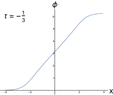
(a)

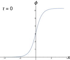
(b)

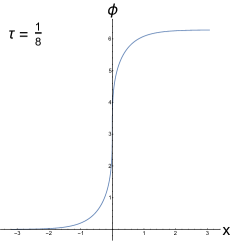
(c)

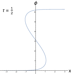
(d)

Figure 1: The $\textsc{T}\bar{\textsc{T}}$-deformed stationary kink solution (49) ($\alpha=1,\beta=0$) for different values of the perturbation parameter $\tau$. The critical value $\tau=1/8$ (c) corresponds to a shock wave singularity.

In Figure 1, the stationary kink-solution is depicted for four different values of the perturbing parameter $\tau$, $\tau=1/8$ corresponds to a shock-wave singularity. Finally, notice that (49) fulfills

$$\begin{cases}{\displaystyle\partial\phi\left(z,\overline{z}\right)=\frac{2\alpha\sin\left(\frac{\phi\left(z,\overline{z}\right)}{2}\right)}{1-4\tau+4\tau\cos\left(\phi\left(z,\overline{z}\right)\right)}},\\ {\displaystyle\overline{\partial}\phi\left(z,\overline{z}\right)=\frac{\frac{2}{\alpha}\sin\left(\frac{\phi\left(z,\overline{z}\right)}{2}\right)}{1-4\tau+4\tau\cos\left(\phi\left(z,\overline{z}\right)\right)}}.\end{cases}\;$$ (50)

Since the $\textsc{T}\bar{\textsc{T}}$ perturbation does not spoil integrability, it is tempting to identify (50) as the first-step Bäcklund transformation from the vacuum solution. Unfortunately, equations (50) do not contain much information about integrability, and the complete form of the Bäcklund transformation is expected to be very complicated. A first, more concrete, step toward a fully satisfactory understanding of the classical integrability of this system will be taken in Section 3.2 below, where the Lax operators are explicitly constructed. Finally, let us conclude this Section with a brief discussion on the more complicated examples within the family of solutions (48). Without much loss in generality we consider only the stationary ($\beta=0$, $\alpha=1$) cases. At $\tau=0$, equation (48) reduces to:

$$x\left(\phi\right)=k\pm\frac{{\bf F}\left(\frac{\phi}{2}|-\frac{1}{\kappa}\right)}{\sqrt{\kappa}}\;\longrightarrow\;\phi\left(x\right)=\pm 2\,\textrm{\bf am}\left(\sqrt{\kappa}\left(x-k\right)\Big{|}-\frac{1}{\kappa}\right)\;,$$ (51)

where $\textrm{\bf am}\left(x\Big{|}k\right)$ is the amplitude of Jacobi elliptic function, they correspond to staircase type solutions, see Figure 2. At $\tau\neq 0$ they display a deformed shape similar to that observed for the single kink solution, with a shock-wave singularities at $\tau\simeq 1/8$.

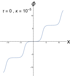
(a)

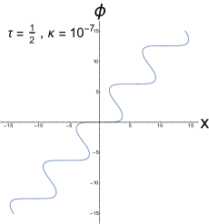
(b)

Figure 2: The general solution (48) for the undeformed (a) and the deformed (b) theory, for small values of $\kappa$.

3.2 Integrability: the $\textsc{T}\bar{\textsc{T}}$-deformed Lax pair

As a first step towards the expression of the Lax operators for the $\textsc{T}\bar{\textsc{T}}$-deformed sine-Gordon model, let us look at the Euler-Lagrange equations in complex coordinates:

$$\partial\left(\frac{\partial\mathcal{L}_{\text{SG}}\left(\phi,\tau\right)}{\partial(\partial\phi)}\right)+\bar{\partial}\left(\frac{\partial\mathcal{L}_{\text{SG}}\left(\phi,\tau\right)}{\partial(\bar{\partial}\phi)}\right)=\frac{\partial\mathcal{L}_{\text{SG}}\left(\phi,\tau\right)}{\partial\phi}\;,$$ (52)

with the Lagrangian given by

$$\mathcal{L}_{\text{SG}}\left(\phi,\tau\right)=\frac{V\left(\phi\right)}{1-\tau V\left(\phi\right)}+\frac{-1+S\left(\phi\right)}{2\tau\left(1-\tau V\left(\phi\right)\right)}\;,\;S(\phi)=\sqrt{1+4\tau\left(1-\tau V\right)\partial\phi\,\bar{\partial}\phi}\;.$$ (53)

The potential $V\left(\phi\right)$ is defined in (30), and from the explicit expression of $S$ (we omit the explicit dependence on $\phi$ hereafter) we see that

$$\frac{\partial S}{\partial\phi}=-\tau\,\frac{V^{\prime}}{1-\tau\,V}\frac{S^{2}-1}{2S}\;,$$ (54)

$$\frac{\partial S}{\partial(\partial\phi)}=\frac{4\tau\left(1-\tau V\right)\bar{\partial}\phi}{2S}\;,\qquad\frac{\partial S}{\partial(\bar{\partial}\phi)}=\frac{4\tau\left(1-\tau V\right)\partial\phi}{2S}\;.$$ (55)

Equation (52) can be immediately recast into the following form

$$\partial\left(\frac{\bar{\partial}\phi}{S}\right)+\bar{\partial}\left(\frac{\partial\phi}{S}\right)=\frac{V^{\prime}}{4S}\left(\frac{S+1}{1-\tau V}\right)^{2}\;.$$ (56)

With this expression for the equations of motion, we can proceed and search for a pair of matrices

$$L=\left(\begin{array}[]{cc}-a&b\\ c&a\end{array}\right)\;,\qquad\bar{L}=\left(\begin{array}[]{cc}\bar{a}&\bar{b}\\ \bar{c}&-\bar{a}\end{array}\right)\;,$$ (57)

such that the zero-curvature condition

$$\partial\bar{L}-\bar{\partial}L=\left[L,\bar{L}\right]\;,$$ (58)

is satisfied iff $\phi$ solves (56). In terms of the Lax pair’s components, (58) is equivalent to the following three equations

$$\partial\bar{a}+\bar{\partial}a=b\bar{c}-c\bar{b}\;,$$ (59a)

$$\bar{\partial}b-\partial\bar{b}=2a\bar{b}+2\bar{a}b\;,$$ (59b)

$$\partial\bar{c}-\bar{\partial}c=2a\bar{c}+2\bar{a}c\;.$$ (59c)

We choose (rather arbitrarily) the first (59a) to correspond exactly to the equation of motion for $\phi$. It is then reasonable to choose

$$a=\gamma\frac{\partial\phi}{2S}\;,\qquad\bar{a}=\gamma\frac{\bar{\partial}\phi}{2S}\;,$$ (60)

with $\kappa$ and arbitrary constant to be determined later. The equations (59) become

$$b\bar{c}-c\bar{b}=\gamma\frac{V^{\prime}}{8S}\left(\frac{S+1}{1-\tau V}\right)^{2}\;,$$ (61a)

$$\bar{\partial}b-\partial\bar{b}=\gamma\frac{\partial\phi}{S}\bar{b}+\gamma\frac{\bar{\partial}\phi}{S}b\;,$$ (61b)

$$\partial\bar{c}-\bar{\partial}c=\gamma\frac{\partial\phi}{S}\bar{c}+\gamma\frac{\bar{\partial}\phi}{S}c\;.$$ (61c)

Now it comes the most tricky part of our construction: determining the form of the remaining functions $b$, $c$, $\bar{b}$ and $\bar{c}$. We can proceed by making a perturbative expansion in $\tau$, solving the equations and trying to recognize some pattern in the terms. Sparing the reader the boring details, one arrives at the following Ansatz:

$$b=\left[\mu e^{\mathbbm{i}\frac{\phi}{2}}B_{+}\left(V,S\right)+\tilde{\mu}e^{-\mathbbm{i}\frac{\phi}{2}}\left(\partial\phi\right)^{2}B_{-}\left(V,S\right)\right]\;,$$ (62a)

$$c=\left[\frac{1}{\tilde{\mu}}e^{-\mathbbm{i}\frac{\phi}{2}}B_{+}\left(V,S\right)+\frac{1}{\mu}e^{\mathbbm{i}\frac{\phi}{2}}\left(\partial\phi\right)^{2}B_{-}\left(V,S\right)\right]\;,$$ (62b)

$$\bar{b}=\left[\tilde{\mu}e^{-\mathbbm{i}\frac{\phi}{2}}B_{+}\left(V,S\right)+\mu e^{\mathbbm{i}\frac{\phi}{2}}\left(\bar{\partial}\phi\right)^{2}B_{-}\left(V,S\right)\right]\;,$$ (62c)

$$\bar{c}=\left[\frac{1}{\mu}e^{\mathbbm{i}\frac{\phi}{2}}B_{+}\left(V,S\right)+\frac{1}{\tilde{\mu}}e^{-\mathbbm{i}\frac{\phi}{2}}\left(\bar{\partial}\phi\right)^{2}B_{-}\left(V,S\right)\right]\;,$$ (62d)

$$\gamma=\frac{\mathbbm{i}}{2}\;.$$ (62e)

Here the parameters $\mu$ and $\tilde{\mu}$ are completely arbitrary complex numbers. They can be, in principle, regarded as two independent spectral parameters. However, as we shortly see, there really exists a single independent spectral parameter, up to global $SL\left(2,\mathbb{C}\right)$ rotation. The expressions above, when inserted into the equations (61), give

$$B_{+}=\frac{\left(S+1\right)^{2}}{8S\left(1-\tau V\right)}\;,\;B_{-}=\frac{\tau}{2S}\;.$$ (63)

We thus arrive to the following form of the Lax pair for the $\textsc{T}\bar{\textsc{T}}$-deformed sine-Gordon model:

$$L=\left(\begin{array}[]{cc}-\mathbbm{i}\frac{\partial\phi}{4S}&\mu e^{\mathbbm{i}\frac{\phi}{2}}\frac{\left(S+1\right)^{2}}{8S\left(1-\tau V\right)}+\tilde{\mu}e^{-\mathbbm{i}\frac{\phi}{2}}\left(\partial\phi\right)^{2}\frac{\tau}{2S}\\ \frac{1}{\tilde{\mu}}e^{-\mathbbm{i}\frac{\phi}{2}}\frac{\left(S+1\right)^{2}}{8S\left(1-\tau V\right)}+\frac{1}{\mu}e^{\mathbbm{i}\frac{\phi}{2}}\left(\partial\phi\right)^{2}\frac{\tau}{2S}&\mathbbm{i}\frac{\partial\phi}{4S}\end{array}\right)\;,\;$$ (66)

$$\bar{L}=\left(\begin{array}[]{cc}\mathbbm{i}\frac{\bar{\partial}\phi}{4S}&\tilde{\mu}e^{-\mathbbm{i}\frac{\phi}{2}}\frac{\left(S+1\right)^{2}}{8S\left(1-\tau V\right)}+\mu e^{\mathbbm{i}\frac{\phi}{2}}\left(\bar{\partial}\phi\right)^{2}\frac{\tau}{2S}\\ \frac{1}{\mu}e^{\mathbbm{i}\frac{\phi}{2}}\frac{\left(S+1\right)^{2}}{8S\left(1-\tau V\right)}+\frac{1}{\tilde{\mu}}e^{-\mathbbm{i}\frac{\phi}{2}}\left(\bar{\partial}\phi\right)^{2}\frac{\tau}{2S}&-\mathbbm{i}\frac{\bar{\partial}\phi}{4S}\end{array}\right)\;.$$ (69)

There is one final manipulation that we wish to perform. As we mentioned above, the presence of two independent spectral parameters $\mu$ and $\tilde{\mu}$ is redundant and we can fix the dependence of the Lax pair on a single parameter $\lambda=\sqrt{\mu/\tilde{\mu}}$ by applying the following global $SL\left(2,\mathbbm{C}\right)$ rotation:

$$L\;\longrightarrow\;\tilde{L}=\mathcal{S}^{-1}L\mathcal{S}\;,\qquad\bar{L}\;\longrightarrow\tilde{\bar{L}}=\mathcal{S}^{-1}\bar{L}\mathcal{S}\;,$$ (70)

where

$$\mathcal{S}=\left(\begin{array}[]{c c}\sqrt{\tilde{\mu}\lambda}&0\\ 0&\frac{1}{\sqrt{\tilde{\mu}\lambda}}\end{array}\right)\equiv\left(\begin{array}[]{c c}\left(\tilde{\mu}\mu\right)^{\frac{1}{4}}&0\\ 0&\left(\tilde{\mu}\mu\right)^{-\frac{1}{4}}\end{array}\right)\;.$$ (71)

We end up with the following expressions (omitting the tildas on the transformed Lax operators)

$$L=\left(\begin{array}[]{cc}-\mathbbm{i}\frac{\partial\phi}{4S}&\lambda e^{\mathbbm{i}\frac{\phi}{2}}\frac{\left(S+1\right)^{2}}{8S\left(1-\tau V\right)}+\frac{1}{\lambda}e^{-\mathbbm{i}\frac{\phi}{2}}\left(\partial\phi\right)^{2}\frac{\tau}{2S}\\ \lambda e^{-\mathbbm{i}\frac{\phi}{2}}\frac{\left(S+1\right)^{2}}{8S\left(1-\tau V\right)}+\frac{1}{\lambda}e^{\mathbbm{i}\frac{\phi}{2}}\left(\partial\phi\right)^{2}\frac{\tau}{2S}&\mathbbm{i}\frac{\partial\phi}{4S}\end{array}\right)\;,\;$$ (74)

$$\bar{L}=\left(\begin{array}[]{cc}\mathbbm{i}\frac{\bar{\partial}\phi}{4S}&\frac{1}{\lambda}e^{-\mathbbm{i}\frac{\phi}{2}}\frac{\left(S+1\right)^{2}}{8S\left(1-\tau V\right)}+\lambda e^{\mathbbm{i}\frac{\phi}{2}}\left(\bar{\partial}\phi\right)^{2}\frac{\tau}{2S}\\ \frac{1}{\lambda}e^{\mathbbm{i}\frac{\phi}{2}}\frac{\left(S+1\right)^{2}}{8S\left(1-\tau V\right)}+\lambda e^{-\mathbbm{i}\frac{\phi}{2}}\left(\bar{\partial}\phi\right)^{2}\frac{\tau}{2S}&-\mathbbm{i}\frac{\bar{\partial}\phi}{4S}\end{array}\right)\;.$$ (77)

Now, by using the following limiting behaviours

$$S\;\underset{\tau\rightarrow 0}{\longrightarrow}\;1\;,\qquad B_{+}\;\underset{\tau\rightarrow 0}{\longrightarrow}\;\frac{1}{2}\;,\qquad B_{-}\;\underset{\tau\rightarrow 0}{\longrightarrow}\;0\;,$$ (78)

we easily verify that, in the vanishing perturbation limit $\tau\rightarrow 0$, we recover, as expected, the usual Lax pair for the sine-Gordon model:

$$L=\left(\begin{array}[]{cc}-\mathbbm{i}\frac{\partial\phi}{4}&\frac{\lambda}{2}e^{\mathbbm{i}\frac{\phi}{2}}\\ \frac{\lambda}{2}e^{-\mathbbm{i}\frac{\phi}{2}}&\mathbbm{i}\frac{\partial\phi}{4}\end{array}\right)\;,\;\bar{L}=\left(\begin{array}[]{cc}\mathbbm{i}\frac{\bar{\partial}\phi}{4}&\frac{1}{2\lambda}e^{-\mathbbm{i}\frac{\phi}{2}}\\ \frac{1}{2\lambda}e^{\mathbbm{i}\frac{\phi}{2}}&-\mathbbm{i}\frac{\bar{\partial}\phi}{4}\end{array}\right)\;.$$ (79)

Therefore, we have proved that the classical integrability of sine-Gordon model survives the $\textsc{T}\bar{\textsc{T}}$ deformation, by displaying the existence of the Lax pair (74). We wish to conclude this Section by remarking that the knowledge of the Lax pair for the $\textsc{T}\bar{\textsc{T}}$-deformed sine-Gordon model comes with two additional results:

• Single boson BI Lax pair, obtained by simply looking at the Euler-Lagrange equations (52) with $V=V^{\prime}=0$:

  $$L=\left(\begin{array}[]{cc}-\mathbbm{i}\frac{\partial\phi}{4S}&0\\ 0&\mathbbm{i}\frac{\partial\phi}{4S}\end{array}\right)\;,\;\bar{L}=\left(\begin{array}[]{cc}\mathbbm{i}\frac{\bar{\partial}\phi}{4S}&0\\ 0&-\mathbbm{i}\frac{\bar{\partial}\phi}{4S}\end{array}\right)\;.$$ (84)

• sinh-Gordon Lax pair, which can be derived from (66) by simply redefining the field $\varphi=\mathbbm{i}\phi$

  $$L=\left(\begin{array}[]{cc}-\frac{\partial\varphi}{4\tilde{S}}&\lambda e^{\frac{\varphi}{2}}\frac{\left(\tilde{S}+1\right)^{2}}{8\tilde{S}\left(1-\tau\tilde{V}\right)}-\frac{1}{\lambda}e^{-\frac{\varphi}{2}}\left(\partial\varphi\right)^{2}\frac{\tau}{2\tilde{S}}\\ \lambda e^{-\frac{\varphi}{2}}\frac{\left(\tilde{S}+1\right)^{2}}{8\tilde{S}\left(1-\tau\tilde{V}\right)}-\frac{1}{\lambda}e^{\frac{\varphi}{2}}\left(\partial\varphi\right)^{2}\frac{\tau}{2\tilde{S}}&\frac{\partial\varphi}{4\tilde{S}}\end{array}\right)\;,\;$$ (87)

  $$\bar{L}=\left(\begin{array}[]{cc}\frac{\bar{\partial}\varphi}{4\tilde{S}}&\frac{1}{\lambda}e^{-\frac{\varphi}{2}}\frac{\left(\tilde{S}+1\right)^{2}}{8\tilde{S}\left(1-\tau\tilde{V}\right)}-\lambda e^{\frac{\varphi}{2}}\left(\bar{\partial}\varphi\right)^{2}\frac{\tau}{2\tilde{S}}\\ \frac{1}{\lambda}e^{\frac{\varphi}{2}}\frac{\left(\tilde{S}+1\right)^{2}}{8\tilde{S}\left(1-\tau\tilde{V}\right)}-\lambda e^{-\frac{\varphi}{2}}\left(\bar{\partial}\varphi\right)^{2}\frac{\tau}{2\tilde{S}}&-\frac{\bar{\partial}\varphi}{4\tilde{S}}\end{array}\right)\;,$$ (90)

  where we introduced

  $$\tilde{V}=2\left(1-\cosh\varphi\right)\;,\;\tilde{S}=\sqrt{1-4\tau\left(1-\tau\tilde{V}\right)\partial\varphi\bar{\partial}\varphi}\;.$$ (91)

This proves that both theories, as expected, retain their integrable structure along the $\textsc{T}\bar{\textsc{T}}$ flow.

4 Maxwell-Born-Infeld electrodynamics in 4D

Two-photon plane wave scattering in 4D Maxwell-Born-Infeld (MBI) electrodynamics was considered by Schrödinger and others in pre-QED times (see, for example, Scharnhorst:2017wzh for a nice historical review on the early period of non-linear electrodynamics theories). Later, in Barbashov:1967zzz ; 1966JETP it was shown that the scattering of two plane waves in MBI electrodynamics can be mapped onto a specific solution of the 2D bosonic BI equations of motion, the $N=2$ model in equations (15) and (16). In particular, it is extremely suggestive that the resulting phase-shift can be nicely interpreted as being the classical analog of the $\textsc{T}\bar{\textsc{T}}$-related scattering phase. Compare, for example, the results of Barbashov:1967zzz ; 1966JETP with the discussion about the classical origin of the time delay in dubovsky2012solving .

Motivated by these observations, in this Section we investigate the 4D MBI theory of electrodynamics and show that interestingly it shares a lot of common aspects with the 2D bosonic BI models studied in Section 2. In particular we will see that it arises as a deformation of the Maxwell theory induced by the square root of the determinant of the Hilbert stress-energy tensor.
Consider the MBI Lagrangian in 4D defined on a generic background metric $g_{\mu\nu}$ as

$$\mathcal{L}^{\textrm{\text{\tiny\bf MBI}}}_{g}(\mathcal{A},\tau)=\frac{-\sqrt{|\det\left[g_{\mu\nu}\right]|}+\sqrt{\det\left[g_{\mu\nu}+\sqrt{2\tau}F_{\mu\nu}\right]}}{2\tau}\;,\;\left(\mu,\nu=\left\{1,2,3,4\right\}\right)\;,$$ (92)

where $F_{\mu\nu}=\partial_{\mu}\mathcal{A}_{\nu}-\partial_{\nu}\mathcal{A}_{\mu}$ is the field strength associated to the abelian gauge field $\mathcal{A}_{\mu}$. In Euclidean spacetime $(g_{\mu\nu}=\eta_{\mu\nu}\equiv\text{diag}(+1,+1,+1,+1))$, (92) takes the form

$$\mathcal{L}^{\textrm{\text{\tiny\bf MBI}}}(\mathcal{A},\tau)=\frac{-1+\sqrt{1-\tau\,\text{Tr}\left[F^{2}\right]+\frac{\tau^{2}}{4}\left(\text{Tr}[F\widetilde{F}]\right)^{2}}}{2\tau}\;,$$ (93)

where $\widetilde{F}_{\mu\nu}=\frac{1}{2}\epsilon_{\mu\nu\rho\sigma}F^{\rho\sigma}$ is the Hodge dual field strength. From the expansion of (93) in powers of $\tau$ around $\tau=0$

$$\mathcal{L}^{\textrm{\text{\tiny\bf MBI}}}(\mathcal{A},\tau) \underset{\tau\rightarrow 0}{\sim} -\frac{1}{4}\textrm{Tr}[F^{2}]+\frac{\tau}{16}\left(\textrm{Tr}[F^{2}]^{2}-4\textrm{Tr}[F^{4}]\right)+\mathcal{O}(\tau^{2})$$ (94)

$$= \mathcal{L}^{\text{\tiny\bf M}}+\tau\sqrt{\det[T^{\text{\tiny\bf M}}]}+\mathcal{O}(\tau^{2})\;,$$

one recognizes the Maxwell Lagrangian

$$\mathcal{L}^{\text{\tiny\bf M}}(\mathcal{A})=\frac{1}{4}F_{\mu\nu}F^{\mu\nu}=-\frac{1}{4}\textrm{Tr}[F^{2}]\;,$$ (95)

at the order $\mathcal{O}(\tau^{0})$. The $\mathcal{O}(\tau)$ contribution in (94) is instead related to the determinant of the Hilbert stress-energy tensor of the Maxwell theory $T^{\text{\tiny\bf M}}$, which can be computed from the Noether theorem adding the Belinfante-Rosenfeld improvement to make it symmetric and gauge invariant, i.e.

$$\left(T^{\text{\tiny\bf M}}\right)^{\mu\nu}\equiv\frac{\partial\mathcal{L}^{\text{\tiny\bf M}}}{\partial\left(\partial_{\mu}\mathcal{A}_{\rho}\right)}F^{\nu\rho}-\eta^{\mu\nu}\mathcal{L}^{\text{\tiny\bf M}}=F^{\mu\rho}F^{\nu\rho}-\eta^{\mu\nu}\mathcal{L}^{\text{\tiny\bf M}}\;.$$ (96)

Formula (94) hints that $\mathcal{L}^{\text{\text{\tiny\bf MBI}}}$ may arise from a deformation of Maxwell electrodynamics effected by the operator $\mathcal{O}\equiv\sqrt{\det[T^{\text{\text{\tiny\bf MBI}}}]}$ according to the flow equation

$$\partial_{\tau}\mathcal{L}^{\text{\text{\tiny\bf MBI}}}=\sqrt{\det[T^{\text{\text{\tiny\bf MBI}}}]}\;,$$ (97)

where $T^{\text{\text{\tiny\bf MBI}}}$ is the Hilbert stress-energy tensor associated to the MBI Lagrangian. Using the general definition

$$\left(T^{\text{\text{\tiny\bf MBI}}}\right)^{\mu\nu}=\frac{-2}{\sqrt{g}}\frac{\delta\mathcal{L}^{\text{\text{\tiny\bf MBI}}}_{g}}{\delta g_{\mu\nu}}\;,\;\sqrt{g}\equiv\sqrt{|\det[g_{\mu\nu}]|}\;,$$ (98)

it is possible to show that, in euclidean spacetime $(g_{\mu\nu}=\eta_{\mu\nu})$, the following relation holds

$$\mathcal{O}=\frac{-1+\mathcal{S}(\tau)-2\tau\,\mathcal{L}^{\text{\tiny\bf M}}}{2\tau^{2}\mathcal{S}(\tau)}=\partial_{\tau}\mathcal{L}^{\text{\text{\tiny\bf MBI}}}\;,\;\mathcal{S}(\tau)\equiv\sqrt{\det\left[\eta_{\mu\nu}+\sqrt{2\tau}F_{\mu\nu}\right]}\;,$$ (99)

thus proving the validity of (97).
As noticed in Baggio:2018gct , the presence of an internal symmetry (in the current case the $U(1)$ gauge symmetry) makes the definition of the stress-energy tensor ambiguous. As already appears at the perturbative level in (94), here the symmetric and gauge invariant Hilbert stress-energy tensor seems to be the natural choice to get the BI Lagrangian as a deformation of the Maxwell electrodynamics. However let us point out that there is no reason to rule out a priori a deformation induced by the Noether stress-energy tensor, which is neither symmetric nor gauge invariant.
Driven by the formal analogy between (93) and the bosonic 2D BI Lagrangian (16), now we apply the same strategy of Section 2 to put interactions in the theory.
Recasting (93) into a more compact form

$$\mathcal{L}^{\textrm{\text{\tiny\bf MBI}}}(\mathcal{A},\tau)=\frac{-1+\sqrt{1+4\tau\,\mathcal{L}^{\text{\tiny\bf M}}(\mathcal{A})+4\tau^{2}\mathcal{B}^{\text{\tiny\bf MBI}}}}{2\tau}\;,\;\mathcal{B}^{\text{\text{\tiny\bf MBI}}}=\det[F]\;,$$ (100)

one immediately see that the quantity

$$\mathcal{L}^{\text{\text{\tiny\bf MBI}}}_{\chi}(\mathcal{A},\tau)=\frac{1}{\chi}\mathcal{L}^{\text{\text{\tiny\bf MBI}}}\left(\mathcal{A},\frac{\tau}{\chi^{2}}\right)\;,$$ (101)

where $\chi$ is again an auxiliary adimensional parameter, satisfies the inhomogeneous Burgers equation

$$\partial_{\tau}\mathcal{L}^{\text{\text{\tiny\bf MBI}}}_{\chi}(\mathcal{A},\tau)=\mathcal{L}^{\text{\tiny\bf MBI}}_{\chi}(\mathcal{A},\tau)\,\partial_{\chi}\mathcal{L}^{\text{\tiny\bf MBI}}_{\chi}(\mathcal{A},\tau)+\frac{\mathcal{B}^{\text{\tiny\bf MBI}}}{\chi^{3}}\;,$$ (102)

with boundary condition

$$\mathcal{L}^{\text{\tiny\bf MBI}}_{\chi}(\mathcal{A},0)=\frac{1}{\chi}\mathcal{L}^{\text{\tiny\bf M}}(\mathcal{A})\;.$$ (103)

Now it is straightforward to introduce interactions in the theory. Starting from a boundary condition of the form

$$\mathcal{L}^{{\text{\tiny\bf MBI},V}}_{\chi}(\mathcal{A},0)=\frac{1}{\chi}\mathcal{L}^{\text{\tiny\bf M}}(\mathcal{A})+\chi\,V(\mathcal{A})\;,$$ (104)

where $V(\mathcal{A})$ is a derivative-independent potential, the solution to (102) becomes

$$\mathcal{L}^{{\text{\text{\tiny\bf MBI}}},V}_{\chi}(\mathcal{A},\tau)=\frac{\chi\,V}{1-\tau\,V}+\frac{\chi}{2\bar{\tau}}\left(-1+\sqrt{\det\left[\eta_{\mu\nu}+\sqrt{\frac{2\bar{\tau}}{\chi^{2}}}F_{\mu\nu}\right]}\right)\;,$$ (105)

where $\bar{\tau}=\tau(1-\tau\,V(\mathcal{A}))$ is the usual (local) redefinition of the deformation parameter. A posteriori it is easy to check that $\mathcal{L}^{{\text{\text{\tiny\bf MBI}}},V}_{\chi=1}(\mathcal{A},\tau)$ is indeed solution to (97), i.e.

$$\sqrt{\det[T^{\text{\text{\tiny\bf MBI}},V}]}=-\frac{\mathcal{S}(\bar{\tau})(2\bar{\tau}\,V-1)-(2\tau\,V-1)\left(1+2\bar{\tau}\,\mathcal{L}^{\text{\tiny\bf M}}\right)}{2\bar{\tau}^{2}\,\mathcal{S}(\bar{\tau})}=\partial_{\tau}\mathcal{L}^{\text{\tiny\bf MBI},V}(\mathcal{A},\tau)\;.$$ (106)

Following Section 2, it is interesting to perform a Legendre transformation on $\mathcal{L}^{\text{\tiny\bf MBI},V}(\mathcal{A},\tau)$ to get the Hamiltonian density $\mathcal{H}^{\text{\tiny\bf MBI},V}(\Pi,\mathcal{A},\tau)$. Again, using a shorthand notation for the time derivative $\dot{\mathcal{A}_{\mu}}=\partial_{4}\mathcal{A}_{\mu}$, the conjugated momentum is

$$\Pi^{i}=\frac{\partial\mathcal{L}^{\text{\tiny\bf MBI},V}(\mathcal{A},\tau)}{\partial\dot{\mathcal{A}}_{i}}\;,\;\Pi^{4}\equiv 0\;,\;(i=1,2,3)\;,$$ (107)

and the Hamiltonian density takes the form

$$\mathcal{H}^{\text{\tiny\bf MBI},V}(\Pi,\mathcal{A},\tau)=\frac{V(\mathcal{A})}{1-\tau\,V(\mathcal{A})}+\frac{1}{2\bar{\tau}}\left(-1+\sqrt{1+4\bar{\tau}\,\mathcal{H}^{\text{\tiny\bf M}}(\Pi,\mathcal{A})+4\bar{\tau}^{2}\,|\vec{\mathcal{P}}^{\text{\tiny\bf MBI}}(\Pi,\mathcal{A})|^{2}}\right)\;,$$ (108)

where $\mathcal{H}^{\text{\tiny\bf M}}(\Pi,\mathcal{A})=-\frac{1}{2}\Pi_{i}\Pi^{i}+\frac{1}{4}F_{ij}F^{ij}=-T^{\text{\tiny\bf M}}_{44}$ is formally the Hamiltonian density of the Maxwell theory and $\mathcal{P}^{\text{\tiny\bf MBI}}_{i}(\Pi,\mathcal{A})=-{\mathbbm{i}}\,T^{\text{\tiny\bf MBI}}_{4i}\;,\;(i=1,2,3)$ , is the $i$-th component of the conserved momentum density of the deformed theory, following the same convention of Section 2. Notice that $\mathcal{H}^{\text{\tiny\bf MBI},V}(\Pi,\mathcal{A},\tau)$ is formally identical to the Hamiltonian density reported in Section (2) for the 2D bosonic theory, and again it satisfies an analogous inhomogeneous Burgers equation.

Furthermore, let us stress that setting a field-independent constant potential $V(\mathcal{A})=F_{0}$, also in this case there exists a special value of the parameter $\tau$, i.e. $\tau_{0}=\frac{1}{2F_{0}}$, such that the determinant of the Hilbert stress-energy tensor takes a constant value

$$\det[T^{\text{\tiny\bf MBI}}(\tau_{0})]=\left(\frac{\pi}{2\bar{\tau}_{0}}\right)^{4}\;,\;\bar{\tau}_{0}=\tau_{0}(1-\tau_{0}\,F_{0})\;.$$ (109)

Finally, we would like to make some comments about the generalization of the $\textsc{T}\bar{\textsc{T}}$ deformation to higher dimensions. Here we found that a 4D theory arises as a deformation induced by a power $1/2$ of the determinant of the stress-energy tensor. This result apparently does not agree with the generalization to higher dimensions proposed in Cardy:2018sdv , from which one would expect a power $1/(D-1)=1/3$ instead. Interestingly, notice also that the operator $\sqrt{\det[T^{\text{\tiny\bf MBI}}]}$ can be written in this form

$$\sqrt{\det[T^{\text{\tiny\bf MBI}}]}=\frac{1}{4}\left(\frac{1}{2}\mathrm{Tr}\left[T^{\text{\tiny\bf MBI}}\right]^{2}-\mathrm{Tr}\left[\left(T^{\text{\tiny\bf MBI}}\right)^{2}\right]\right)\;,$$ (110)

which strongly resembles the generalization of the $\textsc{T}\bar{\textsc{T}}$ operator to higher dimensions recently proposed in Taylor:2018xcy , except for the factor $1/2$ in front of $\mathrm{Tr}\left[T^{\text{\tiny\bf MBI}}\right]^{2}$ instead of $1/(D-1)=1/3$.

Although in this Section we have seen that there are many similarities at the classical level between the 4D Maxwell-Born-Infeld model and the 2D bosonic model discussed in Section 2, the situation at the quantum level is in principle much more complicated. However it would be remarkable if a structure similar to that reviewed in Section 2 could emerge for the quantized energy spectrum.

5 Deformed 2D Yang-Mills

The 4D electrodynamics case turns out to be quite special, since in other dimensions the MBI Lagrangian seems not to arise from a deformation of the Maxwell theory driven by any power of the determinant of the Hilbert stress-energy tensor. Solving perturbatively equation (14), with initial condition the Maxwell Lagrangian at $\tau=0$, only for the two-dimensional case we were able to recover the full analytic expression for the deformed Lagrangian:

$$\mathcal{L}^{\text{\tiny\bf M}_{2}}(\mathcal{A},\tau)=\frac{3}{4\tau}\left(\,{}_{3}F_{2}\left(-\frac{1}{2},-\frac{1}{4},\frac{1}{4};\frac{1}{3},\frac{2}{3};\frac{256}{27}\,\tau\,\mathcal{L}^{\text{\tiny\bf M}_{2}}(\mathcal{A},0)\right)-1\right)\;,$$ (111)

where $\mathcal{L}^{\text{\tiny\bf M}_{2}}(\mathcal{A},0)=\frac{1}{2}F_{21}F^{21}$ is the 2D Maxwell Lagrangian, and $F_{21}=-F_{12}$ is the only non-vanishing component of the field strength. Expression (111) is unexpectedly complicated, however, since the quantized energy spectrum should still satisfy the Burgers equation (1), simplifications may appear at the level of the classical Hamiltonian density. As before, denoting the time derivative as $\dot{\mathcal{A}}_{\mu}=\partial_{2}\mathcal{A}_{\mu}$, the conjugated momenta are

$$\Pi^{1}=\frac{\partial\mathcal{L}^{\text{\tiny\bf M}_{2}}(\mathcal{A},\tau)}{\partial\dot{\mathcal{A}}_{1}}\;,\;\Pi^{2}=0\;,$$ (112)

and the explicit form of the Legendre map can be obtained using the Lagrange inversion theorem to invert the relation (112). One finds that $F_{21}$ can be expressed in terms of $\Pi^{1}$ as

$$F_{21}=\frac{4\Pi^{1}}{\bigl{(}2+\tau\,(\Pi^{1})^{2}\bigr{)}^{2}}\;,$$ (113)

and ”surprisingly” the Hamiltonian density takes a very simple form

$$\mathcal{H}^{\text{\tiny\bf M}_{2}}(\Pi,\tau)=\frac{\mathcal{H}^{\text{\tiny\bf M}_{2}}(\Pi,0)}{1-\tau\,\mathcal{H}^{\text{\tiny\bf M}_{2}}(\Pi,0)}\;,$$ (114)

where $\mathcal{H}^{\text{\tiny\bf M}_{2}}(\Pi,0)=-\frac{1}{2}(\Pi^{1})^{2}=-T^{\text{\tiny\bf M}_{2}}_{22}$ is the 2D Maxwell Hamiltonian. The results (111) and (114) can be straightforwardly generalized to encompass the non-abelian 2D Yang-Mills (YM₂) theory with generic gauge group $G$. In fact, using the following definition for the Hilbert stress-energy tensor of the YM theory

$$\left(T^{\text{\tiny\bf YM}}\right)^{\mu\nu}\equiv\frac{\partial\mathcal{L}^{\text{\tiny\bf YM}}}{\partial\left(\partial_{\mu}\mathcal{A}_{\rho}^{a}\right)}F_{a}^{\nu\rho}-\eta^{\mu\nu}\mathcal{L}^{\text{\tiny\bf YM}}\;,$$ (115)

where $\mathcal{L}^{\text{\tiny\bf YM}}(\mathcal{A}^{a})=\frac{1}{4}F_{\mu\nu}^{a}F_{a}^{\mu\nu}$ is the YM Lagrangian and $F_{\mu\nu}^{a}=\partial_{\mu}\mathcal{A}_{\nu}^{a}-\partial_{\nu}\mathcal{A}_{\mu}^{a}+f^{abc}\mathcal{A}_{\mu}^{b}\mathcal{A}_{\nu}^{c}$ is the field strength associated to the non-abelian gauge field $\mathcal{A}_{\mu}^{a}$, it is easy to prove that the deformed non-abelian Lagrangian and Hamiltonian densities, i.e. $\mathcal{L}^{\text{\tiny\bf YM}_{2}}(\mathcal{A}^{a},\tau)$ and $\mathcal{H}^{\text{\tiny\bf YM}_{2}}(\Pi^{a},\tau)$ , have again the form (111) and (114) respectively with the formal replacement:

$$\mathcal{L}^{\text{\tiny\bf M}_{2}}(\mathcal{A})\rightarrow\mathcal{L}^{\text{\tiny\bf YM}_{2}}(\mathcal{A}^{a})\;,\;\\ \mathcal{H}^{\text{\tiny\bf M}_{2}}(\Pi)\rightarrow\mathcal{H}^{\text{\tiny\bf YM}_{2}}(\Pi^{a})\;,$$ (116)

where $\mathcal{L}^{\text{\tiny\bf YM}_{2}}(\mathcal{A}^{a})=\frac{1}{2}F_{21}^{a}F^{21}_{a}$ and $\mathcal{H}^{\text{\tiny\bf YM}_{2}}(\Pi^{a})=-\frac{1}{2}\Pi^{1\,a}\Pi^{1}_{a}=-T^{\text{\tiny\bf YM}_{2}}_{22}$ are the Lagrangian and Hamiltonian density of YM₂ respectively. Although the deformed Lagrangian is very complicated, the Hamiltonian $\mathcal{H}^{\text{\tiny\bf YM}_{2}}(\Pi^{a},\tau)$ fulfills

$$\partial_{\tau}\mathcal{H}_{\chi}^{\text{\tiny\bf YM}_{2}}(\Pi^{a},\tau)=\mathcal{H}_{\chi}^{\text{\tiny\bf YM}_{2}}(\Pi^{a},\tau)\,\partial_{\chi}\mathcal{H}_{\chi}^{\text{\tiny\bf YM}_{2}}(\Pi^{a},\tau)\;,$$ (117)

with initial condition $\mathcal{H}_{\chi}^{\text{\tiny\bf YM}_{2}}(\Pi^{a},0)=\chi\,\mathcal{H}^{\text{\tiny\bf YM}_{2}}(\Pi^{a})$, which means that $\mathcal{H}^{\text{\tiny\bf YM}_{2}}(\Pi^{a},\tau)$ behaves, under the $\textsc{T}\bar{\textsc{T}}$ deformation, as a pure potential term (cf. Section 2). The latter property can be interpreted as an explicit manifestation of the well known pure topological character of YM₂.

This simple observation directly motivated the following proposal for the deformed versions of the partition functions/heat kernels Migdal:1975zg ; Rusakov:1990rs ; Caselle:1993mq ; Gross:1994ub which is compatible with all known consistency constraints Smirnov:2016lqw ; Cavaglia:2016oda ; Cardy:2018sdv . The partition function of YM₂ defined on an orientable 2D manifold $\mathcal{M}$ with genus $p$ and metric $g_{\mu\nu}$ is

$$Z^{\mathcal{M}}(A)=\int{\cal D}{\cal A}_{\mu}\;e^{-\frac{1}{4\tilde{g}^{2}}\int_{\mathcal{M}}dx^{2}\sqrt{g}\,{\text{T}r}[F_{\mu\nu}^{a}F^{\mu\nu}_{a}]}=\sum_{\mathcal{R}}d_{\mathcal{R}}^{2-2p}e^{-\frac{\tilde{g}^{2}}{2}A\,{\bf C}_{2}(\mathcal{R})}\;,$$ (118)

where we have restored the explicit dependence on the Yang-Mills coupling constant $\tilde{g}$. In (118), $A$ is the total area of $\mathcal{M}$, the sum is over all equivalence classes of irreducible representations ${\cal R}$ of the gauge group $G$, $d_{\mathcal{R}}$ is their dimension and ${\bf C}_{2}(\mathcal{R})$ is the quadratic Casimir in the representation $\mathcal{R}$. The generalization of (118) to a manifold with genus $p$ and $n$ boundaries corresponds to the so-called heat kernel:

$$Z^{\mathcal{M}}(g_{1},\dots,g_{n}|A)=\sum_{\mathcal{R}}d_{\mathcal{R}}^{2-2p-n}\chi_{\mathcal{R}}(g_{1})\dots\chi_{\mathcal{R}}(g_{n})e^{-\frac{\tilde{g}^{2}}{2}A\,{\bf C}_{2}(\mathcal{R})}\;,$$ (119)

where $g_{i}$ are the Wilson loops evaluated along the boundaries, and $\chi_{\mathcal{R}}$ denotes the Weyl character of the representation $\mathcal{R}$. According to (114), the $\textsc{T}\bar{\textsc{T}}$ contribution is then included through a simple redefinition, in the heat kernel (119), of the eigenvalues of the quadratic Casimir operator:

$${\bf C}_{2}(\mathcal{R})\rightarrow{\bf C}_{2}({\cal R},\tau)=\frac{{\bf C}_{2}({\cal R})}{1-\tau\,\frac{\tilde{g}^{2}}{2}\,{\bf C}_{2}({\cal R})}\;,$$ (120)

where the dressed operator ${\bf C}_{2}({\cal R},\tau)$, also fulfills equation (117). Since (119) depends only on the surface area $A$ of the manifold, the deformed version $Z^{\mathcal{M}}(g_{1},\dots,g_{n};\tau|A)$ satisfies

$$-\partial_{\tau}Z^{\mathcal{M}}(g_{1},\dots,g_{n};\tau|A)=A\,\partial_{A}^{2}Z^{\mathcal{M}}(g_{1},\dots,g_{n};\tau|A)\;.$$ (121)

With the prescription (120), all the diffusion-type relations introduced in Cardy:2018sdv (see also Dubovsky:2018bmo ; Datta:2018thy ) for the partition functions on various geometries are automatically fulfilled:

• Cylinder: The cylinder partition function $Z^{\text{Cyl}}(g_{1},g_{2}|A)$ corresponds to the $n=2$, $p=0$ case of (119). Setting $A=RL$, and implementing the prescription (120), $Z^{\text{Cyl}}(g_{1},g_{2};\tau|A)$ trivially satisfies Cardy’s equation:

  $$-\partial_{\tau}Z^{\text{Cyl}}(g_{1},g_{2};\tau|A)=(\partial_{L}-1/L)\partial_{R}Z^{\text{Cyl}}(g_{1},g_{2};\tau|A)\;.$$ (122)

• Torus: The partition function on the torus, $Z^{\text{T}}(A)$ corresponds to the $n=0$, $p=1$ case of (119) with $A=L_{1}L_{2}^{\prime}-L_{2}L_{1}^{\prime}$, while the consistency equation for the deformed partition function is:

  $$-\partial_{\tau}Z^{\text{T}}(\tau|A)=\left[\partial_{L_{1}}\partial_{L_{2}^{\prime}}-\partial_{L_{2}}\partial_{L_{1}^{\prime}}-\frac{1}{A}\left(L_{1}\partial_{L_{1}}+L^{\prime}_{1}\partial_{L^{\prime}_{1}}+L_{2}\partial_{L_{2}}+L^{\prime}_{2}\partial_{L^{\prime}_{2}}\right)\right]Z^{\text{T}}(\tau|A)\;.$$ (123)

• Disk and Cone: In the case of a disk, or more in general of a cone with opening angle $\mathcal{X}$, the deformed partition function $Z^{\text{Cone}}(g_{1};\tau|A)$ corresponding to $n=1$, $p=0$ and area $A=\frac{1}{2}\,\mathcal{X}R^{2}$ satisfies

  $$-\partial_{\tau}Z^{\text{Cone}}(g_{1};\tau|A)=\frac{1}{R}\,\mathcal{X}\partial_{\mathcal{X}}\left(\frac{1}{\mathcal{X}}\partial_{R}Z^{\text{Cone}}(g_{1};\tau|A)\right)\;.$$ (124)

Finally, let us stress again that the modification (120) in (119) is expected to hold in general for any value of $p$ and $n$, possibly leading to a consistent deformation of the whole YM₂ setup.

6 Conclusions

The Maxwell-Born-Infeld model is still playing an important role in modern theoretical physics. It was initially proposed as a generalization of electrodynamics, in the attempt to impose an upper limit on the electric field of a point charge, and it corresponds to the only non-linear extension of Maxwell equations that ensures the absence of birefringence and shock waves. Another important feature of this special non-linear field theory is its electric-magnetic self-duality.

The Maxwell-Born-Infeld theory emerges, from this work, as a natural 4D generalization of the $\textsc{T}\bar{\textsc{T}}$-deformed 2D models, as it shares with them some of the properties that make this perturbation so interesting. There are many aspects that deserve further investigation. First of all, it would be nice to extend the ideas of Cardy:2018sdv to this 4D theory and try to derive an evolution-type equation for the quantum energy spectrum at finite volume.

It would be important to explore the classical and quantum properties of the models corresponding to the deformed Lagrangians (105) and to extend the analysis to more general gauge theories.

Considering the interpretation of the 2D examples within the $AdS_{3}/$CFT₂ framework given in McGough:2016lol , the search for analog deformations that preserve integrability in the ABJM model and $\mathcal{N}=4$ super Yang-Mills, could lead to important progresses in our understanding of quantum gravity.

Investigating, at a deeper level, the geometrical meaning of the $\textsc{T}\bar{\textsc{T}}$ deformation in the 2D setup by continuing the study of classical integrable models started in Section 3 appears to be a more feasible but equally important objective. We have now a good control on the deformed quantum spectrum but we have not yet reached an equally satisfactory level of understanding about the influence that this deformation has on classical solutions such as multi-kink or breather configurations. Adapting Bäcklund’s, Hirota’s and the Inverse Scattering methods to the current setup would correspond to a natural extension of some of the results presented in this paper. Finally, it is important to proceed with some concrete application of the YM₂ heat kernel proposal of Section 5 and in particular with the study of the large N limit, which might display novel physical and mathematical features compared to the unperturbed cases.

References

- (1) A. B. Zamolodchikov, Expectation value of composite field in two-dimensional quantum field theory, hep-th/0401146.
- (2) V. Fateev, S. L. Lukyanov, A. B. Zamolodchikov and A. B. Zamolodchikov, Expectation values of local fields in Bullough-Dodd model and integrable perturbed conformal field theories, Nucl. Phys. B516 (1998) 652–674 [hep-th/9709034].
- (3) Al. B. Zamolodchikov, From tricritical Ising to critical Ising by thermodynamic Bethe ansatz, Nucl. Phys. B358 (1991) 524–546.
- (4) L. Castillejo, R. H. Dalitz and F. J. Dyson, Low’s scattering equation for the charged and neutral scalar theories, Phys. Rev. 101 (1956) 453–458.
- (5) Al. B. Zamolodchikov. Unpublished.
- (6) G. Mussardo and P. Simon, Bosonic type S matrix, vacuum instability and CDD ambiguities, Nucl. Phys. B578 (2000) 527–551 [hep-th/9903072].
- (7) F. A. Smirnov and A. B. Zamolodchikov, On space of integrable quantum field theories, Nucl. Phys. B915 (2017) 363–383 [arXiv:1608.05499].
- (8) T. J. Hollowood, From A(m-1) trigonometric S matrices to the thermodynamic Bethe ansatz, Phys. Lett. B320 (1994) 43–51 [hep-th/9308147].
- (9) F. Ravanini, R. Tateo and A. Valleriani, Dynkin TBAs, Int. J. Mod. Phys. A8 (1993) 1707–1728 [hep-th/9207040].
- (10) S. Dubovsky, R. Flauger and V. Gorbenko, Solving the simplest theory of quantum gravity, Journal of High Energy Physics 2012 (2012), no. 9 1–36.
- (11) S. Dubovsky, R. Flauger and V. Gorbenko, Effective String Theory Revisited, JHEP 09 (2012) 044 [arXiv:1203.1054].
- (12) M. Caselle, D. Fioravanti, F. Gliozzi and R. Tateo, Quantisation of the effective string with TBA, JHEP 07 (2013) 071 [arXiv:1305.1278].
- (13) A. Cavaglià, S. Negro, I. M. Szécésnyi and R. Tateo, -deformed 2D Quantum Field Theories, JHEP 10 (2016) 112 [arXiv:1608.05534].
- (14) L. McGough, M. Mezei and H. Verlinde, Moving the CFT into the bulk with , JHEP 04 (2018) 010 [arXiv:1611.03470].
- (15) G. Turiaci and H. Verlinde, Towards a 2d QFT Analog of the SYK Model, JHEP 10 (2017) 167 [arXiv:1701.00528].
- (16) A. Giveon, N. Itzhaki and D. Kutasov, and LST, JHEP 07 (2017) 122 [arXiv:1701.05576].
- (17) A. Giveon, N. Itzhaki and D. Kutasov, A solvable irrelevant deformation of AdS3/CFT2, JHEP 12 (2017) 155 [arXiv:1707.05800].
- (18) M. Asrat, A. Giveon, N. Itzhaki and D. Kutasov, Holography Beyond AdS, arXiv:1711.02690.
- (19) G. Giribet, -deformations, AdS/CFT and correlation functions, JHEP 02 (2018) 114 [arXiv:1711.02716].
- (20) P. Kraus, J. Liu and D. Marolf, Cutoff AdS3 versus the deformation, arXiv:1801.02714.
- (21) W. Cottrell and A. Hashimoto, Comments on double trace deformations and boundary conditions, arXiv:1801.09708.
- (22) M. Baggio and A. Sfondrini, Strings on NS-NS Backgrounds as Integrable Deformations, arXiv:1804.01998.
- (23) J. P. Babaro, V. F. Foit, G. Giribet and M. Leoni, type deformation in the presence of a boundary, arXiv:1806.10713.
- (24) S. Dubovsky, V. Gorbenko and M. Mirbabayi, Asymptotic fragility, near AdS2 holography and , JHEP 09 (2017) 136 [arXiv:1706.06604].
- (25) S. Dubovsky, V. Gorbenko and G. Hernández-Chifflet, Partition Function from Topological Gravity, arXiv:1805.07386.
- (26) A. Bzowski and M. Guica, The holographic interpretation of -deformed CFTs, arXiv:1803.09753.
- (27) M. Guica, An integrable Lorentz-breaking deformation of two-dimensional CFTs, arXiv:1710.08415.
- (28) S. Chakraborty, A. Giveon and D. Kutasov, deformed and String Theory, arXiv:1806.09667.
- (29) L. Apolo and W. Song, Strings on warped AdS3 via deformations, arXiv:1806.10127.
- (30) J. Cardy, The deformation of quantum field theory as a stochastic process, arXiv:1801.06895.
- (31) S. Datta and Y. Jiang, deformed partition functions, arXiv:1806.07426.
- (32) M. Luscher and P. Weisz, String excitation energies in SU(N) gauge theories beyond the free-string approximation, JHEP 07 (2004) 014 [hep-th/0406205].
- (33) M. Billo, M. Caselle and L. Ferro, The Partition function of interfaces from the Nambu-Goto effective string theory, JHEP 02 (2006) 070 [hep-th/0601191].
- (34) S. Chakraborty, A. Giveon, N. Itzhaki and D. Kutasov, Entanglement Beyond , arXiv:1805.06286.
- (35) W. Donnelly and V. Shyam, Entanglement entropy and deformation, arXiv:1806.07444.
- (36) G. Bonelli, N. Doroud and M. Zhu, -deformations in closed form, arXiv:1804.10967.
- (37) M. Taylor, TT deformations in general dimensions, arXiv:1805.10287.
- (38) R. Tateo, “CDD ambiguity and irrelevant deformations of 2D QFT.” http://www.phys.ens.fr/~igst17/slides/Tateo.pdf. Workshop: IGST-2017 ”Integrability in Gauge and String Theory”, 17th–21st of July 2017, ENS, Paris.
- (39) B. M. Barbashov and N. A. Chernikov, Solution and Quantization of a Nonlinear Two-dimensional Model for a Born-Infeld Type Field, Soviet Journal of Experimental and Theoretical Physics 23 (Nov., 1966) 861.
- (40) B. M. Barbashov and N. A. Chernikov, Scattering of Two Plane Electromagnetic Waves in the Non-Linear Born-Infeld Electrodynamics, Commun, math. Phys. 3 (1966) 313–322.
- (41) A. Zamolodchikov, Thermodynamic Bethe Ansatz in Relativistic Models. Scaling Three State Potts and Lee-Yang Models, Nucl. Phys. B 342 (1990) 695–720.
- (42) S. Dubovsky, V. Gorbenko and M. Mirbabayi, Natural Tuning: Towards A Proof of Concept, JHEP 09 (2013) 045 [arXiv:1305.6939].
- (43) R. Hirota, Exact solution of the sine-gordon equation for multiple collisions of solitons, Journal of the Physical Society of Japan 33 (1972), no. 5 1459–1463.
- (44) L. D. Faddeev, L. A. Takhtajan and V. E. Zakharov, Complete description of solutions of the Sine-Gordon equation, Dokl. Akad. Nauk Ser. Fiz. 219 (1974) 1334–1337. [Sov. Phys. Dokl.19,824(1975)].
- (45) K. Scharnhorst, Photon-photon scattering and related phenomena. Experimental and theoretical approaches: The early period, arXiv:1711.05194.
- (46) A. A. Migdal, Recursion Equations in Gauge Theories, Sov. Phys. JETP 42 (1975) 413.
- (47) B. E. Rusakov, Loop averages and partition functions in U(N) gauge theory on two-dimensional manifolds, Mod. Phys. Lett. A5 (1990) 693–703.
- (48) M. Caselle, A. D’Adda, L. Magnea and S. Panzeri, Two-dimensional QCD on the sphere and on the cylinder, in Proceedings, Summer School in High-energy physics and cosmology: Trieste, Italy, June 15-July 31, 1992, pp. 0245–255, 1993. hep-th/9309107.
- (49) D. J. Gross and A. Matytsin, Some properties of large N two-dimensional Yang-Mills theory, Nucl. Phys. B437 (1995) 541–584 [hep-th/9410054].