Centre-of-mass like superposition of Ornstein–Uhlenbeck processes: a pathway
to non-autonomous stochastic differential equations
and to fractional diffusion

Abstract

We consider an ensemble of Ornstein–Uhlenbeck processes featuring a population of relaxation times and a population of noise amplitudes that characterize the heterogeneity of the ensemble. We show that the centre-of-mass like variable corresponding to this ensemble is statistically equivalent to a process driven by a non-autonomous stochastic differential equation with time-dependent drift and a white noise. In particular, the time scaling and the density function of such variable are driven by the population of timescales and of noise amplitudes, respectively. Moreover, we show that this variable is equivalent in distribution to a randomly-scaled Gaussian process, i.e., a process built by the product of a Gaussian process times a non-negative independent random variable. This last result establishes a connection with the so-called generalized gray Brownian motion and suggests application to model fractional anomalous diffusion in biological systems.

1 Introduction

Let $W^{\kappa}_{t}$, $\kappa\in\{1,2,\ldots,N\}$ be a sequence of Wiener processes $W_{t}^{\kappa}:[0,\infty)\to{\mathbb{R}}$ with ${\mathbb{E}}_{x}[W_{t}^{\kappa}]=0$ and ${\mathbb{E}}_{x}[W_{t}^{\kappa}W_{s}^{\kappa}]=\min(t,s)$. As usual, we denote by ${\mathbb{E}}_{x}$ the expectation with respect to $\mathbb{P}_{x}$ where $x$ is the starting point for the process under consideration.

In this paper we consider the ensemble $\{X^{\kappa}_{t}\}_{\kappa}$ of the Ornstein–Uhlenbeck (OU) processes $X^{\kappa}_{t}:[0,\infty)\to{\mathbb{R}}$ satisfying the stochastic differential equations (SDE)

$$dX^{\kappa}_{t}=-\frac{X^{\kappa}_{t}}{{\tau}^{\kappa}}dt+\sqrt{2\,\sigma^{\kappa}}\,dW_{t}^{\kappa}\,,\quad X^{\kappa}_{0}=x\,,$$ (1)

where, $\forall\,\kappa$, ${\tau}^{\kappa}>0$ and $\sigma^{\kappa}>0$. We call ${\tau}^{\kappa}$ relaxation times and $\sigma^{\kappa}$ noise amplitudes. In particular, the following equivalence in law holds true

$$X^{\kappa}_{t}=e^{-\frac{t}{{\tau}^{\kappa}}}(x+W_{\varphi(t)}^{\kappa}),\quad\kappa=1,2,\ldots,N\,,$$ (2)

where

$$\varphi(t)=\sigma^{\kappa}{\tau}^{\kappa}\left(e^{2t/{\tau}^{\kappa}}-1\right)\,.$$ (3)

Hence, each $X^{\kappa}_{t}$ is a real-valued Gaussian process with ${\mathbb{E}}_{x}(X^{\kappa}_{t})=xe^{-t/{\tau}^{\kappa}}$. The correlation function

$${\mathbb{E}}_{x}[X_{t}^{\kappa}X_{s}^{\kappa}]=e^{-(t+s)/{\tau}^{\kappa}}\min(\varphi(t),\varphi(s))$$ (4)

gives the covariance function

$$C(t,s)=\sigma^{\kappa}{\tau}^{\kappa}\,{\rm{e}}^{-|t-s|/{\tau}^{\kappa}}-(\sigma^{\kappa}{\tau}^{\kappa}+x^{2}){\rm{e}}^{-(t+s)/{\tau}^{\kappa}}\,.$$ (5)

Without loss of generality, we assume that $x=0$ and therefore

$$C(t,s)=\sigma^{\kappa}{\tau}^{\kappa}\,\left({\rm{e}}^{-|t-s|/{\tau}^{\kappa}}-{\rm{e}}^{-(t+s)/{\tau}^{\kappa}}\right)\,.$$ (6)

For a given $\kappa$, the infinitesimal generator $A$ of $X^{\kappa}_{t}$ is therefore

$$Au=-\frac{x}{{\tau}^{\kappa}}\frac{du}{dx}+\sigma^{\kappa}\frac{d^{2}u}{dx^{2}},\quad u\in C_{c}(\mathbb{R},\mathbb{R})\,,$$ (7)

where $C_{c}$ is the set of smooth and compactly supported functions on $\mathbb{R}$. In view of the applications in diffusion problems, in analogy with the Langevin equation (for $\gamma,m>0$) we introduce the mass-like variable $m^{\kappa}>0$ such that

$$\frac{1}{{\tau}^{\kappa}}=\frac{{\gamma}^{\kappa}}{m^{\kappa}}\,,\quad\sqrt{\sigma^{\kappa}}=\frac{\sqrt{\sigma_{0}}}{m^{\kappa}}\,,$$ (8)

where $\sigma_{0}>0$ is a fixed parameter independent of $\kappa$, and, $\forall\,\kappa$, the pair of independent parameters $({\tau}^{\kappa},\sigma^{\kappa})$ in the SDE (1) is now replaced by the pair $({\gamma}^{\kappa},m^{\kappa})$.

In the following, we study the centre-of-mass like process

$$Z_{t}=\sum_{\kappa}\frac{m^{\kappa}}{M}X^{\kappa}_{t}\,,$$ (9)

with $M=\sum_{\kappa}m^{\kappa}$.

We highlight that, because of the center-of-mass like formulation, the process $Z_{t}$ here considered differs from the superposition of OU processes considered for example in Refs. [1, 2] or from the superposition of OU-type processes considered in Refs. [3, 4, 5], and also the type of provided results is different. In particular, in this paper we derive the non-autonomous SDE satisfied by a process equivalent in distribution to the process $Z_{t}$ and more we show also that the process $Z_{t}$ is equivalent in distribution to a randomly-scaled Guassian process, i.e., a process built by the product of a non-negative random variable times a Gaussian process. This last result can be understood in the framework of the so-called generalized grey Brownian motion (ggBm), which can be recovered when the Gaussian process is the fractional Brownian motion. The ggBm is a generalization of the theory of the white noise analysis by introducing non-Gaussian measures of Mittag–Leffler type [6, 7, 8, 9, 10].

Under the physical point of view, the considered system can be understood as a heterogeneous ensemble of Brownian particles, i.e., a system composed of non-identical Brownian particles that differ in their density (mass devided by volume). The study of the centre of mass allows for estimating the average concentration and the momentum of inertia of the ensemble by computing the mean and the mean square displacement, respectively. Such a system can be related to the so-called anomalous diffusion which refers to diffusion processes that, in opposition to Brownian motion, do not show a Gaussian density function of particle displacements and neither a linear growth in time of the mean square displacement. Anomalous diffusion is a widespread phenomenon [11, 12] that requires specific statistical tools [13], that is sometimes related to fractional diffusion [14], and that can be generated by the polydispersity when classical thermodynamics holds [15], i.e., with Gaussian noise as in the present case, or by noises with long-range spatiotemporal correlations with even ”anomalous” thermodynamics [15], i.e., with non-Gaussian noise. In this respect, the derived link between the process $Z_{t}$ and the ggBm allows for perspective applications of the present results to model fractional diffusion in biological systems in view of the promising application of the ggBm in these systems [16, 17].

In the next Section 2, the main theorems are stated and their proofs are given in Section 3. In Section 4, the numerical simulations related to the main results of Section 2 are shown. In Section 5 the conclusions are reported and the application to model anomalous diffusion in biological systems is discussed.

2 Main results

In this Section we present the two main results, i.e., Theorem 1 and Theorem 3, that we obtain for the process $Z_{t}$ defined in (9). The first concerns the determination of the non-autonomous SDE satisfied by a process $Z_{t}^{H}$ that is equivalent in distribution to $Z_{t}$, and the second concerns the equivalence in distribution of the process $Z_{t}$ with a randomly-scaled Gaussian process, i.e., a process defined by the product of a non-negative random variable and a Gaussian process.

We introduce the scaled process

$$Y^{\kappa}_{t}=\frac{X^{\kappa}_{t}}{\sqrt{\sigma^{\kappa}}}\,,$$ (10)

for which

$$\mathbb{P}_{0}(Y^{\kappa}_{t}\in dy)=\int_{\Omega_{\tau}}p^{\kappa}(y;t|\tau)q(d\tau)dy\,,$$ (11)

where the Gaussian density $p^{\kappa}$ is conditioned to ${\tau}^{\kappa}$ and

$$\mathbb{P}(\tau^{\kappa}\in\Omega_{\tau})=\int_{\Omega_{\tau}}q(d\tau)=1.$$ (12)

We assume that $q(d\tau)=q(\tau)d\tau$, that is ${\tau}^{\kappa}$ has population density $q:\mathbb{R}^{+}\supseteq\Omega_{\tau}\mapsto\mathbb{R}^{+}$. We notice that ${\tau}^{\kappa}\stackrel{{\scriptstyle d}}{{=}}\tau$, $\forall\,\kappa$, where $\tau$ is distributed according with $q$. We denote by “$\stackrel{{\scriptstyle d}}{{=}}$” the equality in distribution for random variables.

We maintain the superscript $\kappa$ in (11) although the sequence $X^{\kappa}_{t}$ (and therefore, the sequence (10)) are identically distributed. Indeed, we have that $X^{\kappa}_{t}\stackrel{{\scriptstyle d}}{{=}}X_{t}$ and $p^{\kappa}(y;t|\tau)=\sqrt{\sigma^{\kappa}}v(\sqrt{\sigma^{\kappa}}y;t|\tau)$ where $v(x;t|\tau)dx=\mathbb{P}_{0}(X_{t}\in dx)$.

Theorem 1.

Let $Z_{t}:[0,\infty)\to{\mathbb{R}}$ be the center-of-mass like stochastic process in (9). Then, $Z_{t}\stackrel{{\scriptstyle d}}{{=}}Z^{*}_{t}$ where $Z^{*}_{t}$ satisfies the following non-autonomous SDE

$$dZ_{t}^{*}=-\frac{Z_{t}^{*}}{{\tau}_{\rm{eff}}(t)}dt+\frac{\sqrt{2\sigma_{0}}}{M}\,dW_{t}^{\rm{eff}}\,,\quad Z_{0}^{*}=z\,,$$ (13)

with $\sqrt{\sigma_{0}}=m^{\kappa}\sqrt{\sigma^{\kappa}}$, $dW_{t}^{\rm{eff}}=\sum_{\kappa}dW_{t}^{\kappa}$ such that ${\mathbb{E}}[(dW_{t}^{\rm{eff}})^{2}]=N{\mathbb{E}}[(dW_{t}^{\kappa})^{2}]$, and where $\tau_{\rm{eff}}(t)$ is defined as

$${\tau}_{\rm{eff}}(t)=\left[\frac{\displaystyle{\int_{-\infty}^{+\infty}\int_{\Omega_{\tau}}y^{2}p^{\kappa}(y;t|\tau)q(\tau)\,d\tau dy}}{\displaystyle{\int_{-\infty}^{+\infty}\int_{\Omega_{\tau}}\frac{y^{2}}{\tau^{2}}p^{\kappa}(y;t|\tau)q(\tau)\,d\tau dy}}\right]^{1/2}\,.$$ (14)

We observe that the SDE (13) is non-autonomous because of the dependence on $t$ of the drift coefficient through the function ${\tau}_{\rm{eff}}(t)$, and that the noise amplitude $\sqrt{2\sigma_{0}}/M$ is not a process but a non-negative random variable. The opposite situation with a drift independent of $t$ and the noise amplitude given in terms of a stochastic process has been recently studied in Ref. [18]. By setting

$$\Lambda=\sigma_{0}/M^{2}\,,$$

from (8), we have that $\Lambda$ is an independent non-negative random variable.

Theorem 2.

Let $\{X^{\kappa}_{t}\}_{\kappa}$ be the ensemble defined in (1) and (8). Let $Z_{t}:[0,\infty)\to{\mathbb{R}}$ be the center-of-mass like process defined in (9). Let $Y^{\kappa}_{t}$ be the scaled process in (10). Denote by $B_{t}^{H}:[0,\infty)\to{\mathbb{R}}$ the Gaussian process $B_{t}^{H}\stackrel{{\scriptstyle d}}{{=}}\sqrt{{\mathbb{E}}_{0}[(Y^{\kappa}_{t})^{2}]}\,W_{1}$, $\forall\,\kappa$. Then we have that , $\forall\,t>0$, as $N\to\infty$,

$$\frac{1}{\sqrt{N}}Z_{t}\stackrel{{\scriptstyle d}}{{\to}}\sqrt{\Lambda}\,B_{t}^{H}\,.$$ (15)

Theorem 3.

Let $\{X^{\kappa}_{t}\}_{\kappa}$ be the ensemble defined in (1) and (8). Let $Z_{t}:[0,\infty)\to{\mathbb{R}}$ be the center-of-mass like process defined in (9). Let $Y^{\kappa}_{t}$ be the scaled process in (10). Denote by $B_{t}^{H}:[0,\infty)\to{\mathbb{R}}$ the Gaussian process $B_{t}^{H}\stackrel{{\scriptstyle d}}{{=}}\sqrt{{\mathbb{E}}_{0}[(Y^{\kappa}_{t})^{2}]}\,W_{1}$, $\forall\,\kappa$. Then we have that , $\forall\,t>0$, $\forall\,N>0$,

$$Z_{t}\stackrel{{\scriptstyle d}}{{=}}\sqrt{N\Lambda}\,B_{t}^{H}=Z_{t}^{H}\,.$$ (16)

We observe that since $\Lambda$ is a random variable that is different for any realization of the process $B_{t}^{H}$ and it is independent of $t$, the process $Z_{t}^{H}$ is not the same process studied in Ref. [19].

Lemma 1.

The stochastic process $Z_{t}$ has a non-exponential correlation controlled by the population of ${\tau}^{\kappa}$ distributed according to the density $q(\tau)$. The exponential correlation is recovered in the case $q(\tau)=\delta(\tau-\tau_{0})$.

Proof.

Consider the scaled process

$$Y^{\kappa}_{t}=\frac{X^{\kappa}_{t}}{\sqrt{\sigma^{\kappa}}}\,,$$ (17)

which satisfies the SDE

$$dY^{\kappa}_{t}=-\frac{Y^{\kappa}_{t}}{{\tau}^{\kappa}}dt+\sqrt{2}\,dW^{\kappa}_{t}\,,$$ (18)

then it holds

$$Z_{t}=\frac{\sqrt{\sigma_{0}}}{M}\sum_{\kappa}Y^{\kappa}_{t}\,.$$ (19)

Each stochastic process $Y^{\kappa}_{t}$ is an OU process with exponential correlation (4), i.e., $\displaystyle{{\mathbb{E}}[Y^{\kappa}_{t}Y_{s}^{\kappa}|\tau^{\kappa}]=\tau^{\kappa}\,\left({\rm{e}}^{-|t-s|/\tau^{\kappa}}-{\rm{e}}^{-(t+s)/\tau^{\kappa}}\right)}$, $\forall\,\kappa$, according to (18). The correlation of the process $Z_{t}$ is

$${\mathbb{E}}[Z_{t}Z_{s}] = {\mathbb{E}}\left[\frac{\sigma_{0}}{M^{2}}\,{\mathbb{E}}\left[\sum_{\kappa}Y^{\kappa}_{t}\sum_{\kappa}Y_{s}^{\kappa}\bigg{|}{\tau}^{\kappa}\right]\right]$$ (20)

$$= {\mathbb{E}}\left[\frac{\sigma_{0}}{M^{2}}\,\sum_{\kappa}{\mathbb{E}}\left[Y^{\kappa}_{t}Y_{s}^{\kappa}\big{|}{\tau}^{\kappa}\right]\right]$$

$$= {\mathbb{E}}\left[\frac{\sigma_{0}}{M^{2}}\sum_{\kappa}{\tau}^{\kappa}\,\left({\rm{e}}^{-|t-s|/\tau^{\kappa}}-{\rm{e}}^{-(t+s)/\tau^{\kappa}}\right)\right]$$

$$= {\mathbb{E}}\left[\frac{\sigma_{0}}{M^{2}}\right]\sum_{\kappa}{\mathbb{E}}\left[{\tau}^{\kappa}\,\left({\rm{e}}^{-|t-s|/\tau^{\kappa}}-{\rm{e}}^{-(t+s)/\tau^{\kappa}}\right)\right]$$

$$= N\,{\mathbb{E}}\left[\frac{\sigma_{0}}{M^{2}}\right]\int_{\Omega_{\tau}}\tau\,\left({\rm{e}}^{-|t-s|/\tau}-{\rm{e}}^{-(t+s)/\tau}\right)\,q(d\tau),$$

where, we recall that $\Lambda=\sigma_{0}/M^{2}$ is an independent random variable and ${\tau}^{\kappa}$ are independent and identically distributed. The distribution $q(\tau)$ modifies the classical correlation displayed, $\forall\,\kappa$, by ${\mathbb{E}}[Y^{\kappa}_{t}Y_{s}^{\kappa}\big{|}\tau]$. When $q(\tau)=\delta(\tau-\tau_{0})$, the exponential correlation follows. ∎

From Theorem 3, we have that

$${\mathbb{E}}[Z_{t}Z_{s}]=N{\mathbb{E}}[\Lambda]\,{\mathbb{E}}[B_{t}^{H}B_{s}^{H}]=N{\mathbb{E}}[\Lambda]\,R(t,s)\,,$$ (21)

and then, after re-scaling $N\Lambda\to\Lambda$, the following holds

Lemma 2.

Let $f(\lambda)$, $\lambda\in\Omega_{\lambda}\subseteq{\mathbb{R}}^{+}$, be the density of the non-negative random variable $\Lambda$, then the $n$-dimensional density of $Z_{t}$ is

$$\mathcal{P}(\mathbf{z};R)=\frac{1}{\sqrt{(2\pi\lambda)^{n}\,{\rm det}\,R}}\int_{\Omega_{\lambda}}\exp\left\{-\frac{1}{2\lambda}\,\mathbf{z}^{T}R^{-1}\mathbf{z}\right\}\,f(\lambda)\,d\lambda\,,$$ (22)

where $\mathbf{z}=(z_{1},\dots,z_{n})$ and $R=R(t_{i},t_{j})$, $i,j=1,2,\dots,n$, is the covariance matrix of $B_{t}^{H}$.

Corollary 1.

Let $R(t,t)=t^{2H}$, with $0<H<1$, and $\Lambda\sim f(\lambda)$, then the one-point one-time density function of $Z_{t}$ is

$$\mathcal{P}(z;t)=\frac{1}{\sqrt{4\pi\lambda\,t^{2H}}}\int_{\Omega_{\lambda}}\exp\left\{-\frac{z^{2}}{4\lambda\,t^{2H}}\right\}\,f(\lambda)\,d\lambda\,.$$ (23)

Remark 1.

If $f(\lambda)$ is the density function of $\Lambda$, then from the relation $\Lambda=\sigma_{0}/M^{2}$ we have that the density function of $M$ is

$$g(M)=\frac{2\sigma_{0}}{M^{2}}\,f\!\left(\frac{\sigma_{0}}{M^{2}}\right)\,.$$

Remark 2.

If $m^{\kappa}$, $\kappa\in{\mathbb{N}}$, are independent identically distributed variables according to the distribution $\rho(m)$, then $M=\sum m^{\kappa}$ follows the same distribution, i.e.,

$$g(M)\equiv\rho(m)\,.$$

Corollary 2 (See Theorem 2.1 and Corollary 2.1 in Ref. [20]).

Let $R(t,t)=t^{2\beta/\alpha}$ and $f(\lambda)=K^{-\alpha/2}_{\alpha/2,\beta}(\lambda)$, with [21]

$$K^{-\theta}_{\alpha,\beta}(\lambda)=\frac{1}{2\pi}\int_{-\infty}^{+\infty}{\rm{e}}^{-i\omega\lambda}\left\{\frac{1}{2\pi i}\int_{c-i\infty}^{c+i\infty}{\rm{e}}^{pt}\frac{p^{\beta-1}}{p^{\beta}+\Psi_{\alpha}^{\theta}(\omega)}\,dp\right\}\,d\omega\,,$$ (24)

where $0<\beta<1$, $0<\alpha<2$, $\theta=\min\{\alpha,2-\alpha\}$ and $\Psi_{\alpha}^{\theta}(\omega)=|\omega|^{\alpha}{\rm{e}}^{i({\rm{sgn}}\omega)\theta\pi/2}$, then the one-point one-time density function of $Z_{t}$ is [20]

$$\mathcal{P}(z;t) = \frac{1}{\sqrt{4\pi\lambda\,t^{2\beta/\alpha}}}\int_{0}^{+\infty}\exp\left\{-\frac{z^{2}}{4\lambda\,t^{2\beta/\alpha}}\right\}\,K^{-\alpha/2}_{\alpha/2,\beta}(\lambda)\,d\lambda$$ (25)

$$= \frac{1}{t^{\beta/\alpha}}\,K^{0}_{\alpha,\beta}\left(\frac{|z|}{t^{\beta/\alpha}}\right)\,.$$

The density function $\mathcal{P}(z;t)$ defined in (25) is the kernel of the following space-time fractional diffusion equation [21, 20]

$$\left\{\begin{array}[]{lr}{}_{t}D_{*}^{\beta}\,u={{}_{z}D^{\alpha}_{0}}\,u\,,&{\rm{in}}\,\,\Omega\,,\\ \\ u(z,0)=u_{0}(z)\,,&{\rm{in}}\,\,{\mathbb{R}}\,,\end{array}\right.$$ (26)

with $(z,t)\in\Omega={\mathbb{R}}\times(0,\infty)$, $0<\alpha<2$, $0<\beta<1$, and where ${}_{t}D_{*}^{β}$ is the Caputo time-fractional derivative of order $\beta$ defined through the Laplace transfor pair

$$\int_{0}^{+\infty}{\rm{e}}^{-st}\{{{}_{t}D_{*}^{\beta}}u(z,t)\}\,dt=s^{\beta}\,\widetilde{u}(z,s)-\sum_{j=0}^{m-1}s^{\beta-1-j}\,u^{(j)}(z,0^{+})\,,$$

with $m-1<\beta<m$, $m\in{\mathbb{N}}$, and ${}_{z}D_{\theta}^{\alpha}$ is the Riesz–Feller space-fractional derivative of order $\alpha$, and asymmetry parameter $\theta=\min\{\alpha,2-\alpha\}$, defined through the Fourier transform pair

$$\int_{-\infty}^{+\infty}{\rm{e}}^{+i\xi z}\{{{}_{z}D_{\theta}^{\alpha}}u(z,t)\}\,dz=-|\xi|^{\alpha}\,{\rm{e}}^{i(\rm{sign}\,\xi)\theta\pi/2}\,\widehat{u}(\xi,t)\,.$$

Corollary 3.

The density function $\mathcal{P}(z;t)$ in (25) solves the space-time fractional diffusion equation (26), whose special cases are the time-fractional diffusion ($\alpha=2$), the space-fractional diffusion ($\beta=1$), the neutral fractional diffusion ($\alpha=\beta$) and the classical diffusion ($\alpha=2$, $\beta=1$).

The stochastic process $Z_{t}^{H}$ defined in (16) is built with the same constructive approach adopted by Mura [6] to build up the ggBm [6, 7, 8], i.e., a Gaussian process times a non-negative random variable, and here we call such type processes: randomly-scaled Gaussian processes. The ggBm proposed by Mura is recovered from (16) in the case $B_{t}^{H}$ is the fractional Brownian motion and $\Lambda\sim M_{\beta}(\lambda)$ where $M_{\beta}(\lambda)$, $0<\beta<1$, is the M-Wright/Mainardi function [22, 23], i.e., $M_{\beta}(\lambda)=K^{-1}_{1,\beta}(\lambda)$. Then we have the following

Corollary 4.

Let $R(t,t)=t^{2H}$ and $f(\lambda)=M_{\beta}(\lambda)$, with $0<H<1$ and $0<\beta<1$, then the one-point one-time density function of $Z_{t}$ is [24]

$$\mathcal{P}(z;t) = \frac{1}{\sqrt{4\pi\lambda\,t^{2H}}}\int_{0}^{+\infty}\exp\left\{-\frac{z^{2}}{4\lambda\,t^{2H}}\right\}\,M_{\beta}(\lambda)\,d\lambda$$ (27)

$$= \frac{1}{2\,t^{H}}\,M_{\beta/2}\left(\frac{|z|}{t^{H}}\right)\,.$$

The density function $\mathcal{P}(z;t)$ defined in (27) is the kernel of the following Erdélyi–Kober fractional diffusion equation [24]

$$\left\{\begin{array}[]{lr}\displaystyle\frac{\partial u}{\partial t}=\frac{2H}{\beta}t^{2H-1}\,\mathcal{D}_{2H/\beta}^{\beta-1,1-\beta}\frac{\partial^{2}u}{\partial x^{2}}\,,&{\rm{in}}\,\,\Omega\,,\\ \\ u(z,0)=u_{0}(z)\,,&{\rm{in}}\,\,{\mathbb{R}}\,,\end{array}\right.$$ (28)

with $(z,t)\in\Omega={\mathbb{R}}\times(0,\infty)$, $0<H<1$, $0<\beta<1$, where $\mathcal{D}_{\eta}^{\sigma,\mu}$ is the Erdélyi–Kober fractional derivative defined as follows. Let $n-1<\mu\leq n$, $n\in{\mathbb{N}}$, $\eta>0$, $\gamma\in{\mathbb{R}}$, the Erdélyi–Kober fractional derivative is defined as

$$D^{\gamma,\mu}_{\eta}\,\varphi(t)=\prod_{j=1}^{n}\left(\gamma+j+\frac{1}{\eta}t\frac{d}{dt}\right)(I^{\gamma+\mu,n-\mu}_{\eta}\,\varphi(t))\,,$$

where

$$I^{\gamma,\mu}_{\eta}\,\varphi(t)=\frac{\eta}{\Gamma(\mu)}t^{-\eta(\mu+\gamma)}\int_{0}^{t}\tau^{\eta(\gamma+1)-1}(t^{\eta}-\tau^{\eta})^{\mu-1}\varphi(\tau)\,d\tau\,.$$

Corollary 5.

The density function $\mathcal{P}(z;t)$ in (27) solves a fractional diffusion equation in the Erdélyi–Kober sense (28), whose special cases are the time-fractional diffusion ($\beta=2H$), the Brownian non-Gaussian motion ($2H=1$), the Gaussian non-Brownian motion ($\beta=1$) and the classical diffusion ($\beta=2H=1$).

3 Proofs of Theorems 1, 2 and 3

3.1 Proof of Theorem 1

The stochastic dynamics of the process $Z_{t}$ is governed by

$$dZ_{t}=\sum_{\kappa}\frac{m^{\kappa}}{M}dX^{\kappa}_{t}\,.$$

By remembering the definitions in (8), if we plug (1) into (9), we can derive the following Langevin-type dynamics:

$$dZ_{t} = \frac{1}{M}\sum_{\kappa}\left\{-{\gamma}^{\kappa}X^{\kappa}_{t}dt+\sqrt{2\sigma_{0}}\,dW_{t}^{\kappa}\right\}$$

$$= -\frac{1}{M}\left\{\sum_{\kappa}{\gamma}^{\kappa}X^{\kappa}_{t}\right\}dt+\frac{\sqrt{2\sigma_{0}}}{M}\sum_{\kappa}dW_{t}^{\kappa}\,.$$

We introduce now the scaled process $Y^{\kappa}_{t}=X^{\kappa}_{t}/\sqrt{\sigma^{\kappa}}$, then we have

$$\sum_{\kappa}{\gamma}^{\kappa}\,X^{\kappa}_{t} = \sum_{\kappa}{\gamma}^{\kappa}\sqrt{\sigma^{\kappa}}\,Y^{\kappa}_{t}=\sqrt{\sigma_{0}}\sum_{\kappa}\frac{Y^{\kappa}_{t}}{{\tau}^{\kappa}}$$ (29)

$$\stackrel{{\scriptstyle d}}{{=}} \sqrt{\sigma_{0}}\,\sqrt{\sum_{\kappa}{\mathbb{E}}\left[\left(\frac{Y^{\kappa}_{t}}{{\tau}^{\kappa}}\right)^{2}\right]}\,W_{1}$$

$$= \sqrt{\sigma_{0}}\,\frac{\sqrt{\sum_{\kappa}{\mathbb{E}}\left[\left(\frac{Y^{\kappa}_{t}}{{\tau}^{\kappa}}\right)^{2}\right]}}{\sqrt{\sum_{\kappa}{\mathbb{E}}[(Y^{\kappa}_{t})^{2}]}}\sqrt{\sum_{\kappa}{\mathbb{E}}[(Y^{\kappa}_{t})^{2}]}\,W_{1}$$

$$= \frac{1}{{\tau}_{\rm{eff}}}\,\sqrt{\sum_{\kappa}{\mathbb{E}}[(\sqrt{\sigma_{0}}Y^{\kappa}_{t})^{2}]}\,W_{1}$$

$$= \frac{1}{{\tau}_{\rm{eff}}}\,\sqrt{\sum_{\kappa}{\mathbb{E}}[(m^{\kappa}X^{\kappa}_{t})^{2}]}\,W_{1}$$

$$\stackrel{{\scriptstyle d}}{{=}} \frac{1}{{\tau}_{\rm{eff}}}\sum_{\kappa}m^{\kappa}X^{\kappa}_{t}=M\,\frac{Z_{t}}{{\tau}_{\rm{eff}}}\,,$$

where

$$\frac{1}{{\tau}_{\rm{eff}}}=\frac{\sqrt{\sum_{\kappa}{\mathbb{E}}\left[\left(\frac{Y^{\kappa}_{t}}{{\tau}^{\kappa}}\right)^{2}\right]}}{\sqrt{\sum_{\kappa}{\mathbb{E}}[(Y^{\kappa}_{t})^{2}]}}=\left[\frac{\displaystyle{\int_{-\infty}^{+\infty}\int_{\Omega_{\tau}}\frac{y^{2}}{\tau^{2}}p^{\kappa}(y;t|\tau)q(\tau)\,d\tau dy}}{\displaystyle{\int_{-\infty}^{+\infty}\int_{\Omega_{\tau}}y^{2}p^{\kappa}(y;t|\tau)q(\tau)\,d\tau dy}}\right]^{1/2}\,,$$ (30)

which is a function of time, i.e., $\tau_{\rm{eff}}=\tau_{\rm{eff}}(t)$, with $p^{\kappa}(y;t|\tau)$ the Gaussian densities corresponding to the SDE (18).

In the derivation of (29), the first line follows from (8) and the second from the application of the rule of the sum of Gaussian variables reminding that the process $Y^{\kappa}_{t}$ is Gaussian, see (18). The third line contains the multiplication and division by $\sqrt{\sum_{\kappa}{\mathbb{E}}[(Y^{\kappa}_{t})^{2}]}$ and in the fourth $\tau_{\rm{eff}}$ is introduced and the parameter $\sigma_{0}$ is moved below the square root. The fifth line follows from (8) and, finally, in the sixth line the rule of the sum of Gaussian variables is used again in the first equality and (9) is used to have the last equality.

To conclude, by setting $\sum_{\kappa}dW_{t}^{\kappa}=dW_{t}^{\rm{eff}}$, the stochastic process $Z_{t}$ satisfies the following non-autonomous SDE

$$dZ_{t}=-\frac{Z_{t}}{{\tau}_{\rm{eff}}}dt+\frac{\sqrt{2\sigma_{0}}}{M}\,dW_{t}^{\rm{eff}}\,.$$

3.2 Proof of Theorem 2

By considering the scaled process $Y^{\kappa}_{t}=X^{\kappa}_{t}/\sqrt{\sigma^{\kappa}}$, the stochastic process $Z_{t}$ results to be

$$Z_{t}=\frac{\sqrt{\sigma_{0}}}{M}\sum_{\kappa}Y^{\kappa}_{t}\,.$$

Let us write

$$\overline{Y}_{t}^{N}=\frac{1}{N}\sum_{\kappa=1}^{N}Y^{\kappa}_{t}.$$ (31)

Recall that $Y^{\kappa}_{t}\stackrel{{\scriptstyle d}}{{=}}Y^{1}_{t}$, $\forall\,\kappa$. For $x=0$,

$$\mathbb{E}_{x}[\overline{Y}^{N}_{t}]=x\,\mathbb{E}_{0}\left[\frac{e^{-t/\tau}}{\sqrt{\sigma}}\right]=0\,,$$ (32)

and

$$Var_{0}[\overline{Y}^{N}_{t}]=\frac{1}{N}\,\mathbb{E}_{0}[\tau(1-e^{-2t/\tau})]=\frac{1}{N}\,{\mathbb{E}}_{0}[(Y^{1}_{t})^{2}]\,.$$ (33)

From the Central Limit Theorem, as $N\to\infty$

$$\frac{\overline{Y}^{N}_{t}-\mathbb{E}_{0}[\overline{Y}^{N}_{t}]}{\sqrt{Var_{0}[\overline{Y}^{N}_{t}]}}=\sqrt{N}\frac{\overline{Y}_{t}^{N}}{\sqrt{{\mathbb{E}}_{0}[(Y^{1}_{t})^{2}]}}=\frac{1}{\sqrt{{\mathbb{E}}_{0}[(Y^{1}_{t})^{2}]}}\frac{1}{\sqrt{N}}\sum_{\kappa}Y^{\kappa}_{t}\stackrel{{\scriptstyle d}}{{\to}}W_{1}\,,$$

that is, as $N\to\infty$,

$$\frac{1}{\sqrt{N}}\sum_{\kappa=1}^{N}Y^{\kappa}_{t}\stackrel{{\scriptstyle d}}{{\to}}\sqrt{{\mathbb{E}}_{0}[(Y^{1}_{t})^{2}]}\,W_{1}=B^{H}_{t}\,,\quad\forall\,t>0\,.$$

Finally, by multiplying both side by $\sqrt{\sigma_{0}}/M$, we obtain the following equivalence in distribution

$$\forall\,t>0\,,\quad\frac{1}{\sqrt{N}}Z_{t}\stackrel{{\scriptstyle d}}{{\to}}\frac{\sqrt{\sigma_{0}}}{M}B^{H}_{t}\,,\quad N\to\infty\,.$$ (34)

Moreover, by setting $\sqrt{\sigma_{0}}/M=\sqrt{\Lambda}$, the stochastic process $N^{-\frac{1}{2}}Z_{t}$ is statistically equivalent in the sense of the Central Limit Theorem to the process $\sqrt{\Lambda}\,B_{t}^{H}$, i.e.,

$$\frac{1}{\sqrt{N}}Z_{t}\to\sqrt{\Lambda}\,B_{t}^{H}\,.$$

3.3 Proof of Theorem 3

The proof of Theorem 3 follows by considering the previous theorem. Let us consider the Fourier transforms of both densities. We have that

$$\mathbb{E}_{0}[e^{i\xi Z_{t}}]= \int e^{i\xi z}\frac{d}{dz}\mathbb{P}_{0}(Z_{t}<z)\,dz$$

$$= \int e^{i\xi z}\frac{d}{dz}\mathbb{P}_{0}(\sqrt{\Lambda}B^{H}_{t}<\frac{z}{\sqrt{N}})\,dz$$

$$= \int e^{i\xi\sqrt{N}z}\frac{d}{dz}\mathbb{P}_{0}(\sqrt{\Lambda}B^{H}_{t}<z)\,dz$$

$$= \mathbb{E}_{0}[e^{i\xi\sqrt{N\Lambda}B^{H}_{t}}]\,.$$

4 Numerical simulations

In this Section we show by numerical simulations the equivalence in distribution of the three processes $Z_{t}$ (9), $Z_{t}^{*}$ (13) and $Z_{t}^{H}$ (16) as proved in Theorems 1 and 3. The results of the simulations are shown in Fig. 1 by plotting the density functions of the three processes at different times. Moreover, the insets show the corresponding variances.

The centre-of-mass like process $Z_{t}$ is simulated by using its definition (9) through the process $X_{t}^{\kappa}$, which obeys Eq. (1). We remind, that in (1) the parameters $\tau^{\kappa}$ and $\sigma^{\kappa}$, see Eq. (8), follow the corresponding distributions $q(\tau)$ and $g(\sigma)$. In particular, in Panel a), these distributions are

$$g(\sigma)=-\frac{3}{8}\frac{\sigma^{-3/4}}{\Gamma(-2/3)}\exp\left[-\sigma^{-3/8}\right]\,,\qquad q(\tau)=\exp(-\tau)\,,$$ (35)

where we remind that $\Gamma(-2/3)<0$, and in Panel b)

$$g(\sigma)=\eta\frac{\sigma^{\nu-1}}{\Gamma(\nu/\eta)}\exp(-\sigma^{\eta})\,,\qquad q(\tau)=\frac{\alpha}{\Gamma(1/\alpha)}\frac{1}{\tau}L^{-\alpha}_{\alpha}\left(\tau\right)\,,$$ (36)

where $L^{-\alpha}_{\alpha}\left(\tau\right)$ is the Lévy extremal density and $\nu=0.5$, $\eta=1.3$, $\gamma_{0}=10^{-5}$, $\alpha=0.75$.

The process $Z_{t}^{H}$ is simulated by

$$Z_{t}^{H}=\sqrt{N\Lambda}\,B_{t}^{H}=\sqrt{N\Lambda}\sum_{\kappa}{Y_{t}^{\kappa}}=\frac{\sqrt{N\sigma_{0}}}{M}\sum_{\kappa}{Y_{t}^{\kappa}}\,,$$ (37)

where $Y_{t}^{\kappa}$ obeys Eq. (10).

Finally, the process $Z_{t}^{*}$ is simulated by the SDE

$$dZ_{t}^{*}=-\frac{Z_{t}^{*}}{{\tau}_{\rm{eff}}(t)}dt+\frac{\sqrt{2N\sigma_{0}}}{M}\,dW_{t}\,,$$

where, in analogy with previous cases, we use the properties of the sum of Gaussian variables to set $dW_{t}^{\mathrm{eff}}=\sum_{\kappa}dW_{t}^{\kappa}=\sqrt{N}dW_{t}$. Since we already have the trajectories $Y_{t}^{\kappa}$ that we simulated for the process $Z_{t}^{H}$, for numerical convenience, the computation of $\tau_{\mathrm{eff}}$ is performed according to definition in terms of series given in Eq. (30). Moreover, we set $\sigma_{0}=1/N$ because in the simulations we sum $N$ trajectories.

Simulations support the equivalence in distribution among the three processes, at least for the chosen distributions of the parameters.

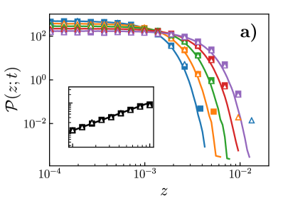
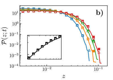
Figure 1: (colour online) Equivalence in distribution of the processes $Z_{t}$ ($\blacksquare$), $Z_{t}^{H}$ ($\vartriangle$) and $Z_{t}^{*}$ (solid lines). Different colours represent different times. Insets: Log-log plots of the variances of the corresponding processes as functions of time. The distributions of the parameters are given with Eq. (35) for Panel a) and Eq. (36) for Panel b).

5 Conclusions and perspectives for applications

In this paper we have considered an ensemble of OU processes characterized by a population of relaxation times and of noise amplitudes. In the framework of the Brownian motion, the OU process can be viewed as a stochastic dynamical equation and is called Langevin equation. In this sense, we have considered a heterogeneous ensemble of Brownian particles.

In particular, we have studied the stochastic dynamics of the centre-of-mass like process of this ensemble and proved that this process is equivalent in distribution to a process generated by a non-autonomous SDE with time-dependent drift term and uncorrelated white noise, i.e., no-memory effects emerge in opposition to approaches based on the generalized Langevin equation or on Langevin equations with coloured noises, and it is equivalent in distribution also to a randomly-scaled Gaussian process, i.e., the product of a Gaussian process times a non-negative random variable.

Moreover we showed that anomalous diffusion emerges as a consequence of the heterogeneity. In fact, we found that the population of the relaxation times contributes to the emergence of an anomalous scaling in time, as shown in (20), and the population of the noise amplitudes contributes to have a non-Gaussian density function (22).

The present study is a further step towards the interpretation of anomalous diffusion as a consequence of a complex environment [25, 16, 20] that is here represented by the heterogeneity of the ensemble of particles. The improvement provided with this paper lays in the fact by using the OU process we establish a relation between the anomalous diffusion and the Brownian motion modelled by the Langevin equation, which is a dynamical equation, so put the emergence of anomalous diffusion on physical basis. Then, future developments will concern the study of the motion and the diffusion properties of a test-particle immersed in a complex environment embodied by such heterogeneous ensemble. This has a direct application for modelling anomalous diffusion [26] and collective motion [27] in biological systems. In fact, anomalous diffusion in biological systems is largely observed in experiments and it is due to macromolecular crowding in the interior of cells and in cellular membranes, because of their densely packed and heterogeneous structures [26, 28]. The proposed modelling approach can be applied for modelling diffusion of meso-scopic test-particle in an environment also composed of meso-scopic particles embodying the heterogeneous and crowded environment where the test-particle moves. The study of diffusion of a test-particle in a heterogeneous and crowed environment motivates future developments of the present research.

References

References

• [1] M. Csörgő, Z. Y. Lin, On moduli of continuity for Gaussian and $l^{2}$-norm squared processes generated by Ornstein–Uhlenbeck processes, Canad. J. Math. 42 (1990) 141–158.
• [2] Z. Y. Lin, On large increments of infinite series of Ornstein–Uhlenbeck processes, Stoch. Process. Appl. 60 (1995) 161–169.
• [3] N. Leonenko, E. Taufer, Convergence of integrated superpositions of Ornstein–Uhlenbeck processes to fractional Brownian motion, Stochastics 77 (6) (2005) 477–499.
• [4] O. E. Barndorff–Nielsen, N. N. Leonenko, Spectral properties of superpositions of Ornstein–Uhlenbeck type processes, Methodol. Comput. Appl. Probab. 7 (2005) 335–352.
• [5] D. Grahovac, N. N. Leonenko, A. Sikorskii, I. Tešnjak, Intermittency of superpositions of Ornstein–Uhlenbeck type processes, J. Stat. Phys. 165 (2016) 390–408.
• [6] A. Mura, Non-Markovian Stochastic Processes and Their Applications: From Anomalous Diffusion to Time Series Analysis, Lambert Academic Publishing, 2011, Ph.D. Thesis, Physics Department, University of Bologna, 2008.
• [7] A. Mura, G. Pagnini, Characterizations and simulations of a class of stochastic processes to model anomalous diffusion, J. Phys. A: Math. Theor. 41 (2008) 285003.
• [8] A. Mura, F. Mainardi, A class of self-similar stochastic processes with stationary increments to model anomalous diffusion in physics, Integr. Transf. Spec. F. 20 (3–4) (2009) 185–198.
• [9] M. Grothaus, F. Jahnert, F. Riemann, J. L. da Silva, Mittag–Leffler analysis I: Construction and characterization, J. Funct. Anal. 268 (2015) 1876–1903.
• [10] M. Grothaus, F. Jahnert, Mittag–Leffler analysis II: Application to the fractional heat equation, J. Funct. Anal. 270 (2016) 2732–2768.
• [11] R. Klages, G. Radons, I. M. Sokolov (Eds.), Anomalous Transport: Foundations and Applications, Wiley–VCH Verlag GmbH & Co. KGaA, Weinheim, 2008.
• [12] J. Klafter, S.-C. Lim, R. Metzler, Fractional Dynamics: Recent Advances, World Scientific, Singapore, 2011.
• [13] Y. Meroz, I. M. Sokolov, A Toolbox for Determining Subdiffusive Mechanisms, Phys. Rep. 573 (2015) 1–29.
• [14] R. Metzler, J. Klafter, The restaurant at the end of the random walk: recent developments in fractional dynamics descriptions of anomalous dynamical processes, J. Phys. A: Math. Theor. 37 (31) (2004) R161–R208.
• [15] S. Gheorghiu, M.-O. Coppens, Heterogeneity explains features of ”anomalous” thermodynamics and statistics, Proc. Natl. Acad. Sci. USA 101 (2004) 15852–15856.
• [16] D. Molina-García, T. Minh Pham, P. Paradisi, C. Manzo, G. Pagnini, Fractional kinetics emerging from ergodicity breaking in random media, Phys. Rev. E 94 (2016) 052147.
• [17] V. Sposini, A. V. Chechkin, F. Seno, G. Pagnini, R. Metzler, Random diffusivity from stochastic equations: comparison of two models for Brownian yet non-Gaussian diffusion, New J. Phys. 20 (2018) 043044.
• [18] F. E. Benth, B. Rüdiger, A. Süss, Ornstein–Uhlenbeck processes in Hilbert space with non-Gaussian stochastic volatility, Stoch. Process. Appl. 128 (2018) 461–486.
• [19] O. Garet, Asymptotic behaviour of Gaussian processes with integral representation, Stoch. Process. Appl. 89 (2000) 287–303.
• [20] G. Pagnini, P. Paradisi, A stochastic solution with Gaussian stationary increments of the symmetric space-time fractional diffusion equation, Fract. Calc. Appl. Anal. 19 (2) (2016) 408–440.
• [21] F. Mainardi, Y. Luchko, G. Pagnini, The fundamental solution of the space-time fractional diffusion equation, Fract. Calc. Appl. Anal. 4 (2) (2001) 153–192.
• [22] F. Mainardi, A. Mura, G. Pagnini, The M-Wright function in time-fractional diffusion processes: A tutorial survey, Int. J. Differ. Equations 2010 (2010) 104505.
• [23] G. Pagnini, The M-Wright function as a generalization of the Gaussian density for fractional diffusion processes, Fract. Calc. Appl. Anal. 16 (2) (2013) 436–453.
• [24] G. Pagnini, Erdélyi–Kober fractional diffusion, Fract. Calc. Appl. Anal. 15 (1) (2012) 117–127.
• [25] G. Pagnini, Short note on the emergence of fractional kinetics, Physica A 409 (2014) 29–34.
• [26] F. Höfling, T. Franosch, Anomalous transport in the crowded world of biological cells, Rep. Prog. Phys. 76 (2013) 046602.
• [27] R. Mayor, S. Etienne-Manneville, The front and rear of collective cell migration, Nat. Rev. Mol. Cell Biol. 17 (2016) 97–109.
• [28] B. M. Regner, D. Vučinić, C. Domnisoru, T. M. Bartol, M. W. Hetzer, D. M. Tartakovsky, T. J. Sejnowski, Anomalous diffusion of single particles in cytoplasm, Biophys. J. 104 (2013) 1652–1660.