A Two-Step Pre-Processing for Semidefinite Programming

Abstract

In semidefinite programming (SDP), a number of pre-processing techniques have been developed, including procedures based on chordal decomposition, which exploit sparsity in the semidefinite program in order to reduce the dimension of individual constraints, and procedures based on facial reduction, which reduces the dimension of the problem by removing redundant rows and columns. So far, these have been studied in isolation. We show that these techniques are, in fact, complementary. In computational experiments, we show that a two-step pre-processing followed by a standard interior-point method outperforms the interior point method, with or without either of the pre-processing techniques, by a considerable margin.

I Introduction

There has been much recent interest in semidefinite programming (SDP), based on the realisation that it provides very tight relaxations for non-convex problems in a variety of domains, including statistics and core machine learning [1, 2, 3], computer vision [4], automatic control [5, 6], and robotics [7]. Often, these instances can be seen as relaxations of certain non-convex polynomial optimisation problems [4, 8, 9, 10, 3].

Instances of semidefinite programming obtained as relaxations of polynomial optimisation problems, among others, are sparse, structured, and strictly feasible (cf. Theorem 3.2 in [10]). One can exploit the structure and sparsity using the so-called chordal decomposition [11, 12, 13, 14, 15, 16], which we introduce formally in the next section. For example, one can use chordal-decomposition in pre-processing [13]. Many examples of the use of chordal-decomposition pre-processing abound in control [6], power systems [17, 18, 19], and statistics [2], but it turns out that such pre-processing can lead to non-trivial numerical issues, as has been recently explained by [20].

Other types of pre-processing can, in fact, address numerical issues. Notably, (partial) facial reduction [21, 22, 23] addresses issues associated with a lack of a strictly feasible point, as defined in the next section. Nevertheless, facial-reduction pre-processing has, so far, attracted much less interest, and has not been used in conjunction with the chordal decomposition, yet.

Here, we introduce a two-step pre-processing for SDP, combining techniques from chordal decomposition and facial reduction. We present extensive numerical results comparing the performance of a standard SDP interior-point method on its own, coupled with chordal-decomposition pre-processing, and coupled with the two-step pre-processing on a variety of large-scale structured instances of SDP, including those arising from the venerable maximum bisection (MAXCUT) problem, a benchmark in binary quadratic programming (BiqMac), a benchmark in power-systems engineering (IEEE Test Cases), and a benchmark in general-purpose semidefinite programming (SDPLib).

Our key observation is that the two-step pre-processing appears does in does improve the performance dramatically, when there is sparsity or structure. Even on SDPLib, which is not know to exhibit any particular structure, considerable improvements are possible. For example, following the two-step pre-processing, SeDuMi, a commonly used open-source interior-point method, solves 50% of a subset of SDPLib, where it is applicable, more than 11 times faster than SeDuMi without pre-processing, in both cases to the same tolerances and on the same hardware and inclusive of the time it takes to perform the pre-processing.

II Background

II-A Semidefinite programming

Let us recall some standard definitions. Consider an optimisation problem over the set $\mathbb{S}^{n}$ of symmetric $n\times n$ matrices:

$$\begin{array}[]{rl}\min_{X\in\mathbb{S}^{n}}&C\bullet X\\ \text{subject to }&A_{i}\bullet X=b_{i},\quad i=1,2,\ldots,m\\ &X\succeq 0\end{array}$$ (4)

where $C,A_{i}\in\mathbb{S}^{n}$ are compatible matrices, $b_{i}\in\mathbb{R}^{n}$ are compatible vectors, $\bullet$ denotes the inner product on $\mathbb{S}^{n}$, i.e., $A\bullet B:=\operatorname{tr}(A^{T}B)=\sum_{{i=1,j=1}}^{n}A_{{ij}}B_{{ij}},$ and $X\succeq 0$ denotes the constraint on matrix $X$ to be positive semi-define, i.e., $v^{T}Xv\geq 0$ for all $v\in\mathbb{R}^{n}$. This problem is known as semidefinite programming. For simplicity, we assume that it is feasible.

As usual, for any convex set $C\subseteq\mathbb{S}^{n}$, a point $X\in\mathbb{S}^{n}$ lies in the relative interior of $C$ if and only if $\forall y\in C,\exists z\in C,\exists\alpha\in R,0<\alpha<1:x=\alpha y+(1-\alpha)z$. The relative interior of the cone of positive semidefinite matrices are the positive definite matrices, i.e., $X$ where $v^{T}Xv>0$ for all $v\in\mathbb{R}^{n}\setminus\{0\}$.

II-B Chordal decomposition

Chordal decomposition is an established pre-processing technique in semidefinite programming, with a history of research going back to 1984 [11], with a considerable revival [13, 24, 25, 20, 26, 27, 16] in the past two decades. It is also known as Matrix Completion Pre-processing or the d-space and r-space Conversion Method [13, 14, 15]. There are important applications in statistics [2], machine learning [28, 29, 3], power systems [17, 18, 19], and automatic control [6]. For an excellent survey, see [24].

Let us define chordal decomposition of (4) with structured $A_{1},\ldots,A_{m}\in S^{n}$ formally. First, let us define the (so-called correlative) sparsity pattern as a simple undirected graph $G=(N,E)$, where $N:=\{1,\ldots,n\}$ and

$$E:=\{(j,k):j\neq k,[A_{i}]_{jk}\neq 0\,\,\,\text{ for some }i=1,\ldots,m\}.$$

Given the sparsity pattern $G(N,E)$ of an SDP, chordal decomposition computes a chordal extension $F$ with $E\subseteq F$, a set of maximal cliques ${C_{1},\ldots,C_{l}}$ of the graph $G(N,F)$, and a clique tree $\mathcal{T}(\mathcal{N},\mathcal{E})$. Using a mapping $\sigma_{s}:\mathbb{N}\to\{1,...,|C_{s}|\}$ (where by $|A|$ we mean the cardinality of set $A$) from the original indices to an ordering of the clique $C_{s}$, we can define:

$$[A_{s,p}]_{\sigma_{s}(i)\sigma_{s}(j)} =\begin{cases}[A_{p}]_{ij}&\text{if}\ s=\min\{t|(i,j)\in\text{C}_{t}\}\\ 0&\text{otherwise}\end{cases}$$ (5)

$$E_{s,ij} =\frac{1}{2}\left(e_{\sigma_{s}(i)}e_{\sigma_{s}(j)}^{T}+e_{\sigma_{s}(j)}e_{\sigma_{s}(i)}^{T}\right)\forall i,j\in\text{C}_{s}$$ (6)

$$(s,t) \in\mathcal{T}\Leftrightarrow(\text{C}_{s},\text{C}_{t})\in\mathcal{E}$$ (7)

Q $$=\text{C}_{s}\cap\text{C}_{t}$$ (8)

with the notation that $e_{\sigma_{s}(i)}\in\mathbb{R}^{|C_{s}|}$.

The SDP is then reformulated using a positive semi-definiteness constraint for each maximal cliques and equality constraints for any vertices in more than one maximal clique:

$$\begin{split}\min_{X_{s}\in\mathbb{S}|\text{C}_{s}|}&\sum_{s=1}^{\ell}A_{s,0}\bullet X_{s}\\ \text{subject to}&\sum_{s=1}^{\ell}A_{s,p}\bullet X^{s}=b_{p}\qquad\forall p=1,\ldots,m\\ &E_{s,ij}\bullet X_{s}=E_{t,ij}\bullet X_{t}\quad\forall i\leq j,i,j\in\text{Q},\\ &\qquad\qquad\qquad\qquad\qquad(s,t)\in\mathcal{E}\\ &X_{s}\succeq 0\qquad\qquad\qquad\quad\forall s=1,\ldots,\ell.\end{split}$$ (9)

II-C Facial reduction

There is also a long history of work on facial reduction [30, 31, 32, 33, 34, 35, 36, 37], another type of pre-processing for SDPs. Facial reduction has been used to pre-process [38, 39] degenerate semidefinite programs. Its applications to machine learning have been limited [40, 41, 42, 43] so far. For a quick overview of facial reduction and its relationship to degeneracy, we refer to [44].

To define facial reduction formally, let us present some facts from convex geometry following [44]. Let us consider a convex cone $\mathcal{K}$ such as $\mathbb{S}^{n}$. A convex cone $F\subset\mathcal{K}$ is called a face of $\mathcal{K}$, when $x,y\in\mathcal{K},x+y\in F\implies x,y\in F$. A face of $\mathcal{K}$ is called proper, if it is neither empty, nor $\mathcal{K}$ itself. Clearly, the intersection of an arbitrary collection of faces of $\mathcal{K}$ is itself a (possibly lower-dimensional) face of $\mathcal{K}$. Non-trivially, the relative interiors of all faces of $\mathcal{K}$ form a partition of $\mathcal{K}$, i.e., every point in $\mathcal{K}$ lies in the relative interior of precisely one face and any proper face of $\mathcal{K}$ is disjoint from the relative interior of $\mathcal{K}$.

Next, let us consider the dual of $\mathcal{K}$, and denote it by $\mathcal{K}^{*}$. We use $\mathcal{K}^{\perp}$ for the orthogonal complement of the affine hull of $\mathcal{K}$. Any set of the form $F=v^{\perp}\cap\mathcal{K}$, for some $v\in\mathcal{K}^{*}$, is called an exposed face of $\mathcal{K}$ with an exposing vector $v$. It is well-known (Proposition 2.2.1 in [44]) that if faces $F_{1},F_{2}\subset\mathcal{K}$ are exposed by vectors $v_{1},v_{2}\in\mathcal{K}^{*}$, then the intersection $F_{1}\cap F_{2}$ is exposed by $v_{1}+v_{2}$. Finally, a convex cone is exposed if all its faces are exposed.

In the case of $\mathbb{S}^{n}$, and its dual $\mathbb{S}^{n}$ (self-duality), there is a correspondence between $r$-dimensional linear subspaces $\mathcal{R}$ of $\mathbb{R}^{n}$ and faces of $\mathbb{S}^{n}$, wherein $F_{\mathcal{R}}:=\{X\in\mathbb{S}^{n}\textrm{ such that range }X\subseteq\mathcal{R}\}$ is a face of $\mathbb{S}^{n}$. Consequently, for any matrix $V\in\mathbb{R}^{n\times r}$ with range $V$ equal to $\mathcal{R}$, we have $F_{\mathcal{R}}=V\mathbb{S}^{r}V^{T}$, i.e., the face is isomorphic to an $r$-dimensional positive semi-definite cone $\mathbb{S}^{r}$. Subsequently, the $F_{\mathcal{R}}$ is being exposed by some $UU^{T}$ for $U\in\mathbb{R}^{n\times(n-r)}$.

In facial reduction, one considers an instance of (4), where the Slater condition fails, and iteratively constructs an equivalent instance, which has a Slater point. In each iteration, one aims to find $y$ such that:

$$\sum_{i=0}^{m}y_{i}A_{i}\succeq 0\textrm{ and }b\bullet y=0.$$ (TEST)

If no such vector $y$ exists, the Slater condition holds by the Theorem of the Alternative (Theorem 3.1.2 in [44]). Otherwise, we know that the minimal face containing the feasible set is contained in $\mathcal{K^{\prime}}:=(\sum_{i=0}^{m}y_{i}A_{i})^{\perp}\cap\mathcal{K}$, which yields an equivalent:

$$\min_{X\in\mathcal{K^{\prime}}} C\bullet X$$ (FR)

subject to $$A_{i}\bullet X=b_{i},\quad i=1,2,\ldots,m$$

$$X\in\mathcal{K^{\prime}}$$

This leaves only the small matter of an efficient implementation.

III An Algorithm

TwoStep($C$, $A_{i}$, $b_{i}$)

$(G(N,E),\mathcal{T}(\mathcal{N},\mathcal{E}))=$ Sparsity($C,A_{1},A_{2},\ldots,A_{m}$)
$(A,E,Q)$ = Reorder by (5), (6), (7), (8)
Let $F_{0}$ be the feasible set of (9)
Let $y_{0}=0,\,i=1.$
repeat
	if no $y$ satisfying (TEST) with $F_{i-1}$ exists, break
	else choose	$y_{i}\in L\cap F_{i-1}^{*}.$
		Compute (SVD)
		Let $F_{i}=F_{i-1}\cap y_{i}^{\perp}$, defined by (SDP-FR)
	Let	$i=i+1.$
end
return $F_{i-1}$

Algorithm 1 A “two-step” pre-processing for an instance $C$, $A_{i}$, $b_{i}$ of semidefinite programming (4).

In Algorithm 1, we suggest that our pre-processing has two steps, at a high level: chordal embedding and facial reduction.

In more detail, there are several substeps to the first step. As a first substep, we may wish to compute a fill-reducing ordering of the matrices. In Matlab, for instance, function amd can be used to compute an approximate minimum degree permutation vector for a sparse matrix, which could be obtained as the union of support sets of the matrices $C$ and $A_{i},i=1,2,\ldots,m$. We note that this substep can be omitted, if necessary, without compromising the results of our analysis below. As a second substep, we compute the chordal embedding. In Matlab, for instance, function symbfact returns the sparsity pattern of the Cholesky factor as its fifth output, which is a widely used embedding. Based on the chordal embedding, one can list all maximal cliques by breadth-first search. That is, cliques forms a clique for each vertex together with its neighbors that follow in a perfect elimination ordering, and tests whether the set of cliques is maximal. Finally, we construct the new semidefinite program (9) based on the cliques $C$.

Subsequently, we run the iterative facial reduction, where we interweave substeps of testing whether to continue with vector $y$ obtained in (TEST) and reducing the instance by computing the singular-value decomposition (SVD) of the positive semidefinite $\sum_{i=0}^{m}y_{i}A_{i}$ to obtain:

$$\begin{bmatrix}U&V\end{bmatrix}\begin{bmatrix}D&0\\ 0&0\end{bmatrix}\begin{bmatrix}U&V\end{bmatrix}^{T},$$ (SVD)

where $[UV]\in\mathbb{R}^{n_{i-1}\times n_{i-1}}$ is an orthogonal matrix with $n_{i-1}$ being the dimension of the $F_{i-1}$ in the previous substep, and $D\in\mathbb{S}^{r}$ is a diagonal matrix. The simplified $F_{i}$ is then:

$$\min_{X^{\prime}\in\mathbb{S}^{n_{i-1}-r}} V^{T}CV\bullet X^{\prime}$$ (SDP-FR)

subject to $$A_{i}\bullet V^{T}X^{\prime}V=b_{i},\quad i=1,2,\ldots,m$$

$$X^{\prime}\succeq 0,$$

where $n_{i-1}$ is, again, the dimension in the previous substep. Notice that in each iteration $r>0$, and hence there can be at most $n$ iterations.

It is not immediately obvious that algorithm TwoStep, Algorithm 1, is efficient. Indeed, reorder and embed solve an NP-Hard problem [45] and we solve a number of non-trivial optimisation problems (TEST) and (FR).

First, notice that algorithm TwoStep does not require the minimum fill-in reordering or embedding:

Proposition 1 (Based on [46])

There is an implementation of embed, which in a graph $R$ with maximum degree $d$ and minimum fill-in $k$ produces a solution within a factor of $O(d^{2.5}\log^{4}(kd))$ of the optimum in time $O(knm+\min(n^{2}M(k)/k,nM(n))$, where $M(n)$ denotes the number of operations needed to multiply two $n\times n$ Boolean matrices.

This is a reasonably tight result, considering that even a constant-factor approximation is NP-Hard, cf. Theorem 21 in [47], exact algorithms cannot run within time $2^{O(\sqrt{n}/\log^{c}n)}$ assuming the Exponential Time Hypothesis, and a variety of lower bounds [48]. We note that there are also algorithms [49] producing fill-in $k$, which is optimal, albeit not running in polynomial time.

Second, notice that:

Proposition 2

For a polynomial-time reorder and embed, Algorithm TwoStep runs in time polynomial in $n$ and $m$ on the BSS machine.

Proof:

The proof is trivial, once one notices that any facial-reduction algorithm solves at most $n$ instances of (FR) in at most $n$ iterations of the seemingly infinite loop, as explained in Section 4.2 in [44]. ∎

Notice, however, that this result reasons about the behaviour of BSS machine [50], rather than the more usual Turing machine, due to the complexity of numerical routines involved, SVD or otherwise.

IV Numerical results

In this section we compare the reliability and speed of interior-point method SeDuMi without any pre-processing, with the chordal-decomposition pre-processing (implemented using SparseCoLO of [51, 52]), and both chordal-decomposition and facial-reduction pre-processing (implemented using SparseCoLO and frlib of [53]). We chose SeDuMi as compared to other solvers due to its overall robustness [54] and the reported complementary performance of this algorithm with FR [55]. The tests were performed on a computing cluster, using 4 cores running at 3 GHz and memory allocated as necessary, running MATLAB 2018b on Debian.

Our conjecture was that especially for sparse structured SDP, chordal-decomposition improves the speed of convergence for some problems, while producing problems too poorly structured for interior-point solvers to solve quickly and reliably. In contrast, the additional facial-reduction step corrects this, and ultimately results in an improved performance overall, compared to both other settings.

We report some of the results as performance profiles. These were introduced in [56] as a way of visualizing the dual performance measures of robustness (solving the largest proportion of problems), and efficiency (solving them quickly). The level of each curve at the right-hand vertical boundary indicates how many problems were solved, and the relative location of each curve compared to the others in the profile intermediately indicates the speed of convergence compared to the best solver for each problem. Simply put, the further to the upper left corner a curve corresponding to an algorithm is, the better.

IV-A SDPLib

Our main experiment considers the SDPLib test set [57], which is a standard for benchmarking SDP software [54], composed of a variety of toy, academic, and real-world SDP problems. These are known to be sparse, but no particular structure is shared across the test set. We refer to http://plato.asu.edu/ftp/sparse_sdp.html for details of the instances and the results obtained by a variety of both free and commercial solvers. Note that out of the 92 instances within the test set, leading solvers can solve 56–88 instances, within a 40000-second (11-hour) time limit per instance considered by [54].

Rather surprisingly, we can demonstrate that one can improve the performance of SeDuMi, an open-source implementation of the interior-point method, which can work with instances without a Slater point. Fig. 1 presents a performance profile [56] on 49 of the 92 instances, where running SparseCoLo did not report a failure. The corresponding numerical values are available from Tab. I: for instance, SeDuMi can solve 50% of instances within 2.89 seconds without any pre-processing, or within 0.19 seconds with the two-step pre-processing. In both cases, the run is to the same tolerances on the same hardware, inclusive of the time it takes to perform the pre-processing. Overall, we found that each step of pre-processing does improve the speed of convergence of the interior-point method in this test set. The reliability does seem to worsen, perhaps as a result of ill-conditioning of the linear systems employed in the interior-point method, after the chordal-decomposition pre-processing. Still, the proportion of the problems solved is very high among this test set, and the strong increase in the speed due to the two-step pre-processing is an indication of the strength of the approach.

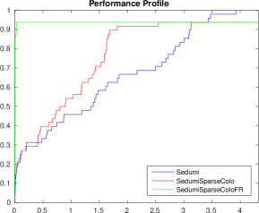
Figure 1: Performance profiles (i.e., proportion of instances from a test set solved over time, relative to the best performer, cf. [56]) comparing SeDuMi with no (Sedumi), chordal-decomposition (SedumiSparseColo), and two-step processing (SedumiSparseColoFR) on 49 instances from SDPLib.

TABLE I: Run-time in seconds of SeDuMi with no, chordal-completion (w/ SC), and two-step (w/ SC+FR) processing, which has been required to solve a certain proportion of instances in SDPLib, up to the tolerances considered by Mittelmann [54]. Dash (–) indicates the run did not finish.

Proportion solved	SeDuMi	w/ SC	w/ SC+FR
$25\%$	$0.48$	$0.23$	$0.084$
$50\%$	$2.29$	$0.69$	$0.19$
$75\%$	$5.07$	$2.79$	$2.8$
$94\%$	$28$	$41$	$40$
$100\%$	$43$	$-$	$-$

IV-B Polynomial optimisation

Next, we illustrate the results on instances from a well-known polynomial optimisation problem (POP). In particular, the so called Lavaei-Low relaxation [19] of the alternating-current optimal power flows (ACOPF) has been shown [17] to coincide with the first level of the moment-SOS hierarchy [58] for POP. Due to the fact that real-life electricity transmission systems are sparse, there is sparsity present in the instances as well, which is widely solved with SparseCoLo pre-processing or related methods [17, 18, 19]. In our test, we consider the well-known IEEE test systems. In the name of the instance, case$x$ denotes a test system on $x$ buses, with more than $4x^{2}$ elements in the moment matrix, P denotes the primal SDP, and D denotes the dual SDP. Tab. II presents the wall-clock run-time (including pre-processing) for 16 such SDP instances. For larger instances (case118 and case300), the two-step pre-processing yields about 2 orders of magnitude of improvement. This is further illustrated by performance profiles on the two sets of problems in Fig. 2: the nearly vertical lines are for the pre-processing, while the nearly horizontal line is without the pre-processing. This set of problems give the clearest indication of the benefits of two step pre-processing, suggesting they are particularly structured to take advantage of the procedures.

TABLE II: Run-time in seconds of SeDuMi with no, chordal-completion (w/ SC), and two-step (w/ SC+FR) processing on instances from polynomial optimisation. Above mid-rule, the instances are in the primal form, below in their dual form.

Instance	SeDuMi	w/ SC	w/ SC+FR
case9	$3.47e^{+02}$	$6.40$	$4.59$
case14	$2.74e^{+01}$	$2.46$	$1.63$
case30	$3.36e^{+01}$	$1.49$	$1.10$
case39	$3.04e^{+01}$	$2.21$	$2.02$
case57	$5.18$	$4.09e^{-01}$	$4.04e^{-01}$
case118	$8.10e^{+03}$	$2.06e^{+01}$	$1.35e^{+01}$
case300	$6.77e^{+01}$	$1.39$	$1.10$
case9	$2.57e^{+02}$	$4.83$	$2.74$
case14	$2.92e^{+01}$	$2.19$	$1.99$
case30	$2.63e^{+01}$	$1.16$	$8.08e^{-01}$
case39	$3.01e^{+01}$	$1.89$	$1.53$
case57	$6.62$	$4.75e^{-01}$	$3.37e^{-01}$
case118	$4.48e^{+03}$	$1.44e^{+01}$	$9.89$
case300	$4.50e^{+01}$	$1.09$	$6.45e^{-01}$

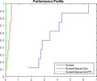
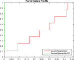
Primal	(Primal, zoomed-in)
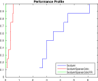
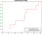
Dual	(Dual, zoomed-in)

Figure 2: Performance profiles (i.e., proportion of instances from a test set solved over time, relative to the best performer, cf. [56]) comparing SeDuMi with no (Sedumi), chordal-decomposition (SedumiSparseColo), and two-step processing (SedumiSparseColoFR) on instances from polynomial optimisation.

TABLE III: Run-time in seconds of SeDuMi with no, chordal-completion (w/ SC), and two-step (w/ SC+FR) processing on instances of the maximum cut problem from the BiqMac benchmark, with and without pre-processing.

N	m	IPM	w/ SC	w/ SC+FR
50	50	$2.22$	$7.49e^{-01}$	$3.38e^{-01}$
100	100	$4.74e^{-01}$	$F$	$F$
150	150	$7.87e^{-01}$	$F$	$F$
200	200	$1.30$	$F$	$F$
300	300	$1.44e^{+01}$	$8.52$	$7.56$
350	350	$1.20e^{+01}$	$1.18e^{+01}$	$1.18e^{+01}$
400	400	$1.45e^{+01}$	$1.45e^{+01}$	$1.44e^{+01}$
450	450	$1.99e^{+01}$	$1.99e^{+01}$	$1.99e^{+01}$
500	500	$3.37e^{+01}$	$3.40e^{+01}$	$3.34e^{+01}$
250	250	$4.62$	$4.58$	$4.54$
250	250	$4.63$	$4.56$	$4.52$
250	250	$4.27$	$4.26$	$4.20$
250	250	$4.77$	$4.72$	$4.65$
250	250	$4.96$	$4.95$	$4.87$

IV-C Binary quadratic programming

Next, let us present results on perhaps the best-known SDP relaxation, that of binary quadratic programming or, equivalently, the maximum cut problem, (MAXCUT). In Tab. III, we see runtime values for SeDuMi by itself, with matrix completion pre-processing, and with the entire two-step pre-processing procedure. We indicate the size of the instance from the BiqMac benchmark as well. We notice that the chordal-decomposition pre-processing sometimes results in a failure of SeDuMi, which could be attributed to numerical failures due to degeneracy. In that case, facial reduction does not improve upon the situation. On small instances in the BiqMac benchmark, there is a small but consistent improvement in the overall run-time, indicating that the pre-processing does improve the efficiency. On larger instances, the differences seem more pronounced.

V Conclusions

Many practically-relevant instances of semidefinite programming are sparse and structured. Traditional general-purpose implementations of exploiting the structure [13, 14, 15] have proven difficult to apply, due to the numerical issues they introduce [20].

While one could try to exploit the structure directly, in custom code, we suggest that general-purpose pre-processing combining both the traditional chordal-decomposition techniques [13, 14, 15] and facial reduction may make it possible to exploit the structure, while relying on the robustness of standard interior-point methods, unaware of the structure.

We have demonstrated that on SDPLib and several sets of structured problems, our combination of chordal completion and facial reduction appears to improve the performance drastically.

VI ACKNOWLEDGEMENTS

Support for this work was provided by the OP VVV project CZ.02.1.01/0.0/0.0/16_019/0000765 “Research Center for Informatics"

References

- [1] A. D’aspremont, L. E. Ghaoui, M. I. Jordan, and G. R. Lanckriet, “A direct formulation for sparse pca using semidefinite programming,” in Advances in Neural Information Processing Systems 17, L. K. Saul, Y. Weiss, and L. Bottou, Eds. MIT Press, 2005, pp. 41–48.
- [2] J. Dahl, L. Vandenberghe, and V. Roychowdhury, “Covariance selection for nonchordal graphs via chordal embedding,” Optimization Methods & Software, vol. 23, no. 4, pp. 501–520, 2008.
- [3] M. A. Erdogdu, Y. Deshpande, and A. Montanari, “Inference in graphical models via semidefinite programming hierarchies,” in Advances in Neural Information Processing Systems 30, I. Guyon, U. V. Luxburg, S. Bengio, H. Wallach, R. Fergus, S. Vishwanathan, and R. Garnett, Eds. Curran Associates, Inc., 2017, pp. 417–425.
- [4] G. Schweighofer and A. Pinz, “Globally optimal o(n) solution to the pnp problem for general camera models,” in The British Machine Vision Conference (BMVC), 2008, pp. 1–10.
- [5] S. Boyd, L. El Ghaoui, E. Feron, and V. Balakrishnan, Linear matrix inequalities in system and control theory. Philadelphia, PA: SIAM Press, 1994, vol. 15.
- [6] Y. Zheng, R. P. Mason, and A. Papachristodoulou, “Scalable design of structured controllers using chordal decomposition,” IEEE Transactions on Automatic Control, vol. 63, no. 3, pp. 752–767, March 2018.
- [7] J. Heller, D. Henrion, and T. Pajdla, “Hand-eye and robot-world calibration by global polynomial optimization,” in 2014 IEEE International Conference on Robotics and Automation (ICRA), May 2014, pp. 3157–3164.
- [8] J. Lavaei and S. H. Low, “Zero duality gap in optimal power flow problem,” IEEE Transactions on Power Systems, vol. 27, no. 1, pp. 92–107, Feb 2012.
- [9] H. Waki, “How to generate weakly infeasible semidefinite programs via lasserre’s relaxations for polynomial optimization,” Optimization Letters, vol. 6, no. 8, pp. 1883–1896, 2012.
- [10] J. Nie and J. Demmel, “Sparse sos relaxations for minimizing functions that are summations of small polynomials,” SIAM Journal on Optimization, vol. 19, no. 4, pp. 1534–1558, 2009.
- [11] B. Grone, C. Johnson, E. Marques de Sa, and H. Wolkowicz, “Positive definite completions of partial Hermitian matrices,” Linear Algebra and its Applications, vol. 58, pp. 109–124, 1984.
- [12] J. R. Blair and B. Peyton, “An introduction to chordal graphs and clique trees,” in Graph theory and sparse matrix computation. Springer, 1993, pp. 1–29.
- [13] M. Fukuda, M. Kojima, K. Murota, and K. Nakata, “Exploiting sparsity in semidefinite programming via matrix completion i: General framework,” SIAM Journal on Optimization, vol. 11, no. 3, pp. 647–674, 2001.
- [14] S. Kim and M. Kojima, Exploiting Sparsity in SDP Relaxation of Polynomial Optimization Problems. Boston, MA: Springer US, 2012, pp. 499–531.
- [15] D. Bergman, C. H. Cardonha, A. A. Cire, and A. U. Raghunathan, “On the Minimum Chordal Completion Polytope,” ArXiv e-prints, 2016.
- [16] Y. Zheng, G. Fantuzzi, A. Papachristodoulou, P. Goulart, and A. Wynn, “Chordal decomposition in operator-splitting methods for sparse semidefinite programs,” Mathematical Programming, vol. 180, no. 1, pp. 489–532, 2020.
- [17] B. Ghaddar, J. Marecek, and M. Mevissen, “Optimal power flow as a polynomial optimization problem,” IEEE Transactions on Power Systems, vol. 31, no. 1, pp. 539–546, Jan 2016.
- [18] M. S. Andersen, A. Hansson, and L. Vandenberghe, “Reduced-complexity semidefinite relaxations of optimal power flow problems,” IEEE Transactions on Power Systems, vol. 29, no. 4, pp. 1855–1863, July 2014.
- [19] S. H. Low, “Convex relaxation of optimal power flow – part i: Formulations and equivalence,” IEEE Transactions on Control of Network Systems, vol. 1, no. 1, pp. 15–27, March 2014.
- [20] A. U. Raghunathan and A. V. Knyazev, “Degeneracy in maximal clique decomposition for semidefinite programs,” in 2016 American Control Conference (ACC), July 2016, pp. 5605–5611.
- [21] J. M. Borwein and H. Wolkowicz, “Facial reduction for a cone-convex programming problem,” Journal of the Australian Mathematical Society (Series A), vol. 30, no. 03, pp. 369–380, 1981.
- [22] M. Liu and G. Pataki, “Exact duality in semidefinite programming based on elementary reformulations,” SIAM Journal on Optimization, vol. 25, no. 3, pp. 1441–1454, 2015.
- [23] G. Pataki, “Bad semidefinite programs: they all look the same,” SIAM Journal on Optimization, 2017.
- [24] L. Vandenberghe and M. S. Andersen, “Chordal graphs and semidefinite optimization,” Foundations and Trends® in Optimization, vol. 1, no. 4, pp. 241–433, 2015.
- [25] Y. Zheng, G. Fantuzzi, A. Papachristodoulou, P. Goulart, and A. Wynn, “Fast admm for semidefinite programs with chordal sparsity,” in 2017 American Control Conference (ACC), May 2017, pp. 3335–3340.
- [26] ——, “Cdcs: Cone decomposition conic solver, version 1.1,” 2016.
- [27] Y. Zheng, “Chordal sparsity in control and optimization of large-scale systems,” Ph.D. dissertation, University of Oxford, 2019.
- [28] M. J. Wainwright and M. I. Jordan, “Treewidth-based conditions for exactness of the sherali-adams and lasserre relaxations,” Technical Report 671, University of California, Berkeley, Tech. Rep., 2004.
- [29] ——, “Graphical models, exponential families, and variational inference,” Foundations and Trends® in Machine Learning, vol. 1, no. 1–2, pp. 1–305, 2008.
- [30] N. Krislock and H. Wolkowicz, “Explicit sensor network localization using semidefinite representations and facial reductions,” SIAM Journal on Optimization, vol. 20, no. 5, pp. 2679–2708, 2010.
- [31] Y.-L. Cheung, “Preprocessing and reduction for semidefinite programming via facial reduction: Theory and practice,” Ph.D. dissertation, University of Waterloo, 2013. [Online]. Available: http://orion.math.uwaterloo.ca/%7Ehwolkowi/henry/reports/thesisvrisnov13.pdf
- [32] F. N. Permenter and P. A. Parrilo, “Basis selection for sos programs via facial reduction and polyhedral approximations,” in 53rd IEEE Conference on Decision and Control, Dec 2014, pp. 6615–6620.
- [33] D. Drusvyatskiy, N. Krislock, Y.-L. C. Voronin, and H. Wolkowicz, “Noisy Euclidean distance realization: robust facial reduction and the Pareto frontier,” SIAM Journal on Optimization, vol. 27, no. 4, pp. 2301–2331, 2017.
- [34] X. Ye, “Low rank matrix completion through semi-definite programming with facial reduction,” Master’s thesis, University of Waterloo, 2016. [Online]. Available: http://www.math.uwaterloo.ca/~hwolkowi//henry/reports/xinghangthesis.pdf
- [35] F. N. Permenter, “Reduction methods in semidefinite and conic optimization,” Ph.D. dissertation, Massachusetts Institute of Technology, 2017.
- [36] F. N. Permenter and P. A. Parrilo, “Partial facial reduction: simplified, equivalent sdps via approximations of the psd cone,” Mathematical Programming, Jun 2017.
- [37] H. Hu, R. Sotirov, and H. Wolkowicz, “Facial reduction for symmetry reduced semidefinite programs,” arXiv preprint arXiv:1912.10245, 2019.
- [38] Y.-L. Cheung, S. Schurr, and H. Wolkowicz, “Preprocessing and regularization for degenerate semidefinite programs,” in Computational and analytical mathematics, ser. Springer Proc. Math. Stat. Springer, New York, 2013, vol. 50, pp. 251–303. [Online]. Available: http://dx.doi.org.proxy.lib.uwaterloo.ca/10.1007/978-1-4614-7621-4_12
- [39] D. Drusvyatskiy, G. Li, and H. Wolkowicz, “A note on alternating projections for ill-posed semidefinite feasibility problems,” Mathematical Programming, vol. 162, no. 1-2, Ser. A, pp. 537–548, 2017.
- [40] B. Alipanahi, N. Krislock, A. Ghodsi, and H. Wolkowicz, “Large-scale manifold learning by semidefinite facial reduction,” University of Waterloo, Waterloo, Ontario, Tech. Rep., 2012. [Online]. Available: http://hal.archives-ouvertes.fr/hal-00684488
- [41] S. Huang and H. Wolkowicz, “Low-rank matrix completion using nuclear norm with facial reduction,” Journal of Global Optimization, vol. to appear, 2017.
- [42] G. Reid, F. Wang, and H. Wolkowicz, “Finding maximum rank moment matrices by facial reduction on primal form and Douglas-Rachford iteration,” ACM Communications in Computer Algebra, vol. 51, no. 1, pp. 35–37, May 2017.
- [43] S. Ma, F. Wang, L. Wei, and H. Wolkowicz, “Robust principal component analysis using facial reduction,” to appear, 2018.
- [44] D. Drusvyatskiy and H. Wolkowicz, “The many faces of degeneracy in conic optimization,” Foundations and Trends® in Optimization, vol. 3, no. 2, pp. 77–170, 2017.
- [45] M. Yannakakis, “Computing the minimum fill-in is np-complete,” SIAM Journal on Algebraic Discrete Methods, vol. 2, no. 1, pp. 77–79, 1981.
- [46] A. Natanzon, R. Shamir, and R. Sharan, “A polynomial approximation algorithm for the minimum fill-in problem,” SIAM Journal on Computing, vol. 30, no. 4, pp. 1067–1079, 2000.
- [47] H. Bodlaender, J. Gilbert, H. Hafsteinsson, and T. Kloks, “Approximating treewidth, pathwidth, frontsize, and shortest elimination tree,” Journal of Algorithms, vol. 18, no. 2, pp. 238 – 255, 1995.
- [48] Y. Cao and R. Sandeep, “Minimum fill-in: Inapproximability and almost tight lower bounds,” in Proceedings of the Twenty-Eighth Annual ACM-SIAM Symposium on Discrete Algorithms. SIAM, 2017, pp. 875–880.
- [49] F. V. Fomin and Y. Villanger, “Subexponential parameterized algorithm for minimum fill-in,” SIAM Journal on Computing, vol. 42, no. 6, pp. 2197–2216, 2013.
- [50] L. Blum, F. Cucker, M. Shub, and S. Smale, Complexity and Real Computation. Secaucus, NJ, USA: Springer-Verlag New York, Inc., 1998.
- [51] K. Fujisawa, S. Kim, M. Kojima, Y. Okamoto, and M. Yamashita, “User’s manual for sparsecolo: Conversion methods for sparse conic-form linear optimization problems,” Research Report B-453, Dept. of Math. and Comp. Sci. Japan, Tech. Rep., pp. 152–8552, 2009.
- [52] S. Kim, M. Kojima, M. Mevissen, and M. Yamashita, “Exploiting sparsity in linear and nonlinear matrix inequalities via positive semidefinite matrix completion,” Mathematical programming, vol. 129, no. 1, pp. 33–68, 2011.
- [53] F. Permenter and P. Parrilo, “Partial facial reduction: simplified, equivalent sdps via approximations of the psd cone,” Mathematical Programming, pp. 1–54, 2014.
- [54] H. D. Mittelmann, “An independent benchmarking of sdp and socp solvers,” Mathematical Programming, vol. 95, no. 2, pp. 407–430, 2003.
- [55] F. Permenter, H. A. Friberg, and E. D. Andersen, “Solving conic optimization problems via self-dual embedding and facial reduction: a unified approach,” SIAM Journal on Optimization, vol. 27, no. 3, pp. 1257–1282, 2017.
- [56] E. D. Dolan and J. J. Moré, “Benchmarking optimization software with performance profiles,” Mathematical Programming, vol. 91, no. 2, pp. 201–213, Jan 2002.
- [57] B. Borchers, “Sdplib 1.2, a library of semidefinite programming test problems,” Optimization Methods and Software, vol. 11, no. 1-4, pp. 683–690, 1999.
- [58] M. F. Anjos and J. B. Lasserre, Handbook on Semidefinite, Conic and Polynomial Optimization. Boston, MA: Springer US, 2012.