Nonlinear spectral analysis of Peregrine solitons observed in optics and in hydrodynamic experiments

Abstract

The data recorded in optical fiber Kibler et al. (2010) and in hydrodynamic Chabchoub et al. (2011) experiments reported the pioneering observation of nonlinear waves with spatiotemporal localization similar to the Peregrine soliton are examined by using nonlinear spectral analysis. Our approach is based on the integrable nature of the one-dimensional focusing nonlinear Schrödinger equation (1D-NLSE) that governs at leading order the propagation of the optical and hydrodynamic waves in the two experiments. Nonlinear spectral analysis provides certain spectral portraits of the analyzed structures that are composed of bands lying in the complex plane. The spectral portraits can be interpreted within the framework of the so-called finite gap theory (or periodic inverse scattering transform). In particular, the number $N$ of bands composing the nonlinear spectrum determines the genus $g=N-1$ of the solution that can be viewed as a measure of complexity of the space-time evolution of the considered solution. Within this setting the ideal, rational Peregrine soliton represents a special, degenerate genus $2$ solution. While the fitting procedures employed in Kibler et al. (2010) and Chabchoub et al. (2011) show that the experimentally observed structures are quite well approximated by the Peregrine solitons, nonlinear spectral analysis of the breathers observed both in the optical fiber and in the water tank experiments reveals that they exhibit spectral portraits associated with more general, genus $4$ finite-gap NLSE solutions. Moreover, the nonlinear spectral analysis shows that the nonlinear spectrum of the breathers observed in the experiments slowly changes with the propagation distance, thus confirming the influence of unavoidable perturbative higher order effects or dissipation in the experiments.

I Introduction

Nonlinear integrable partial differential equations (PDEs) represent an important class of wave equations that are relevant to many fields of physics and applied mathematics Yang (2010); Akhmediev and Ankiewicz (1997); Ablowitz (2011). Notable examples include the one-dimensional nonlinear Schrödinger equation (1D-NLSE), the Korteweg de Vries (KdV) equation and the Benjamin-Ono equation. These integrable PDEs can be solved by using the Inverse Scattering Transform (IST) method Zakharov and Shabat (1972); Ablowitz et al. (1974), and they exhibit soliton solutions, the most celebrated one being the propagation-invariant hyperbolic secant soliton first discovered by Zabusky and Kruskal through numerical simulations of the KdV equation Zabusky and Kruskal (1965); Trillo et al. (2016). Solitons represent solutions of fundamental importance that have the remarkable property to interact elastically and to preserve (asymptotically) their shape and velocity upon nonlinear interactions with other solitons Yang (2010).

Besides fundamental solitons that live on a zero intensity background, the 1D-NLSE with a self-focusing nonlinearity is known to exhibit a special class solutions named breathers or solitons on finite background (SFB). Some prototypical SFB solutions of the focusing 1D-NLSE like the Peregrine soliton (PS), the Kuznetsov-Ma (KM) soliton or the Akhmediev breather (AB) were found around the 80’s Kuznetsov (1977); Ma (1979); Peregrine (1983); Akhmediev et al. (1985). These specific SFB have been experimentally observed in a series of optics and hydrodynamic experiments that have been realized about thirty years later, around 2010 Kibler et al. (2010, 2012); Hammani et al. (2011a); Chabchoub et al. (2011, 2014). The localization properties of those SFB have recently attracted significant interest in the context of studies related to the formation of rogue waves (RWs), a topic of great interest in current experimental and theoretical research Onorato et al. (2013). In particular, the PS exhibits properties of localization both in space and time that make it a particularly attractive model of RWs Shrira and Geogjaev (2010). Even though the PS represents a solution of the 1D-NLSE that may emerge from the process of the development of modulation instability of a plane wave, recent works have demonstrated that the PS also represents a universal nonlinear coherent structure that emerges from the local regularization of a gradient catastrophe Dubrovin et al. (2009); Bertola and Tovbis (2013); Tikan et al. (2017). Note that in addition to the PS, there is an infinite hierarchy of higher-order breather solutions of the 1D-NLSE that are localized both in space and time while having a high peak amplitude Akhmediev et al. (2009a, b). These higher-order SFB solutions have been observed in some recent optics and hydrodynamic experiments Frisquet et al. (2013); Chabchoub et al. (2012a, b). Also, some “superregular solitonic solutions” which appear as small localized perturbations of a plane wave at a certain moment of time have been shown to describe a possible scenario of the nonlinear stage of the modulation instability of the plane wave Zakharov and Gelash (2013); Kibler et al. (2015). Another scenario of the development of modulational instability induced by a localized perturbation theoretically described in Biondini and Mantzavinos (2016) was recently observed in a fiber optic experiment Kraych et al. (2018).

In most of the experiments that have reported so far the observation of SFBs, the signal to noise ratio is so good that it is fully appropriate to compare the traces recorded experimentally with the analytical expression describing the SFB that has been measured. As a result, in most of the hydrodynamic and optics experiments, the discrepancy between the analytical expression and the experimental data is so small that it is naturally concluded that features typifying the SFB under interest have been indeed experimentally observed Kibler et al. (2010, 2012); Chabchoub et al. (2011, 2014); Frisquet et al. (2013); Chabchoub et al. (2012a, b); Kibler et al. (2015). Although the situation is less straigtforward, similar studies have also been realized in experiments or numerical simulations where the breather-like structures may emerge randomly in space and time from some random initial condition. The question of the identification of these breather-like structures represents an issue of importance in the field of integrable turbulence Zakharov (2009); Randoux et al. (2014); Walczak et al. (2015); Agafontsev and Zakharov (2015); Randoux et al. (2016a, 2017); Soto-Crespo et al. (2016); Akhmediev et al. (2016). In this context, fitting procedures have been extensively employed in attempts to identify breather structures that emerge from a randomly fluctuating background Dudley et al. (2014); Akhmediev et al. (2009b, c); Toenger et al. (2015); Walczak et al. (2015); Suret et al. (2016); Närhi et al. (2016); Tikan et al. (2018).

In this paper, we use nonlinear spectral analysis as a mathematical tool to examine the nature of the PS-identified events that have been observed in optics and hydrodynamic experiments reported in ref. Kibler et al. (2010) and Chabchoub et al. (2011). Our approach, which is based on the integrable nature of the 1D-NLSE, consists in computing a spectral (IST) portrait of the experimentally observed coherent structure that is considered as a local solution of the propagation equation. Even though the coherent structures experimentally observed in ref. Kibler et al. (2010) and Chabchoub et al. (2011) are reasonably well fitted by the rational mathematical expression defining the PS, they are found to display spectral signatures that depart from the spectral signature typifying the pure PS defined by its rational mathematical expression. The noticeable distortions that are evidenced by the spectral IST analysis arise from the small discrepancies existing between experimental signals and the ideal mathematical expression defining the PS (see Eq. (11)). Even though the PSs experimentally observed retain some degree of proximity with the pure PS, the spectral analysis reveals that they represent more complex solutions of the 1D-NLSE that can be expressed using Riemann theta functions in the framework of the finite-gap theory Osborne (2010).

This paper is organized as follows. Sec. II.1 introduces the theoretical framework and describes the mathematical tools of nonlinear spectral analysis that are based on the inverse scattering method. Sec. II.2 presents the numerical methods that are used to practically implement nonlinear spectral analysis of SFBs. Sec. III and Sec. IV present the results obtained from the nonlinear spectral analysis of PS-like coherent structures observed in optics Kibler et al. (2010) and hydrodynamic Chabchoub et al. (2011) experiments, respectively. A brief summary and a conclusion of our work are given in Sec. V.

II The inverse scattering transform method for the nonlinear spectral analysis of the Peregrine soliton

II.1 Theoretical framework

We consider the integrable focusing 1D-NLSE in the following form:

$$i\psi_{t}+\psi_{xx}+2\,|\psi|^{2}\,\psi=0,$$ (1)

where $\psi(x,t)$ represents the complex envelope of the optical or hydrodynamical wave fields.

In the experiments considered in Sec. III and in Sec. IV, the evolution variable is not the time $t$ but the longitudinal coordinate $z$ measuring the propagation distance along the optical fiber or along the $1D-$flume. At a given position inside the fiber or inside the flume, the field does not change in space $x$ but in time $t$. Therefore the 1D-NLSE governing wave propagation inside the fiber or inside the 1D-flume is obtained by performing the following changes of variables: $t\leftrightarrow z$, $x\leftrightarrow t$ together with appropriate scaling of the NLSE coefficients with parameters typifying either optics or hydrodynamic experiments Chabchoub et al. (2015); Chabchoub and Grimshaw (2016), see Appendix A and B.

In the IST method, the focusing 1D-NLSE is represented as a compatibility condition of two linear equations Zakharov and Shabat (1972),

$$Y_{x}=\begin{pmatrix}-i\xi&\psi\\ -\psi^{*}&i\xi\\ \end{pmatrix}Y=Q(x,t,\xi)\,Y,$$ (2)

$$Y_{t}=\begin{pmatrix}-2i\xi^{2}+i|\psi|^{2}&i\psi_{x}+2\xi\psi\\ i\psi_{x}^{*}-2\xi\psi^{*}&2i\xi^{2}-i|\psi|^{2}\\ \end{pmatrix}Y,$$ (3)

where $\xi$ is a (time-independent) complex spectral parameter and $Y(x,t,\xi)$ is a vector. The spatial linear operator (2) and the temporal linear operator (3) form the Lax pair of Eq. (1). For a given potential $\psi(x,t)$ the problem of finding the spectrum $\sigma[\psi]$ and the corresponding scattering solution $Y$ specified by the spatial equation (2) is called the Zakharov-Shabat (ZS) scattering problem Yang (2010). The ZS problem is formally analogous to calculating the Fourier coefficients in Fourier theory of linear systems.

Reformulating Eq. (2) as

$$\begin{pmatrix}\partial_{x}+i\xi&-\psi\\ \psi^{*}&\partial_{x}-i\xi\\ \end{pmatrix}Y={\mathcal{L}}^{(x)}Y=0,$$ (4)

every NLSE solution $\psi$, which rapidly decay as $|x|\to\infty$, is characterized by the spectrum $\sigma[\psi]=\{\xi\in\mathbb{C}|\mathcal{L}^{(x)}Y=0,|Y|\,\text{bounded}\,\forall x\}$ of the linear operator $\mathcal{L}^{(x)}$. The discrete eigenvalues of the ZS operator $\mathcal{L}^{(x)}$ with decaying potentials give spectral portraits that provide precise IST signatures of fundamental soliton solutions of Eq. (1) that exponentially decay to zero as $|x|\to\infty$ Yang (2010), while the continuous spectrum component of $\psi$ lies on the real axis.

SFBs are not solutions of Eq. (1) that decay to zero as $|x|\to\infty$ but they rather generically represent certain limits of periodic or quasi-periodic solutions of Eq. (1) obtained in the framework of the extension of IST called the finite-gap theory Tracy et al. (1984); Osborne (2010); Grinevich and Santini (2017). For periodic boundary conditions, i.e. $\psi(x+L,t)=\psi(x,t)\,\forall t$, the spectrum has to be determined from Floquet spectral theory Eastham (1973). In this framework, the spectrum of $\psi$ is expressed in terms of the transfer matrix $M(x+L;\psi,\xi)$ across a period, where $M(x;\psi,\xi)$ is a fundamental solution matrix of the Lax pair. Introducing the Floquet discriminant $\Delta(\psi,\xi)=Tr[M(x+L;\psi,\xi)]$ as the trace of the transfer matrix, the (Floquet) spectrum of a solution of Eq. (1) fulfilling periodic boundary conditions is given by Ablowitz et al. (2001); Islas and Schober (2005); Calini and Schober (2012)

$$\sigma[\psi]=\{\xi\in\mathbb{C}|\Delta(\psi,\xi)\in\mathbb{R},-2\leqslant\Delta(\psi,\xi)\leqslant 2\}$$ (5)

The Floquet spectrum of a periodic solution of Eq. (1) typically consists of bands lying in the complex plane. The number $N$ of these bands determines the genus $g=N-1$ of the finite-gap solution. The genus $g$ solution can be represented in the form:

$$\psi_{g}(x,t)=q\frac{\Theta_{g}(x,t,{\bf\nu_{-}^{0})}}{\Theta_{g}(x,t,{\bf\nu_{+}^{0}})}e^{iq^{2}t}$$ (6)

where $q\in\mathbb{R}$ and $\Theta_{g}$ is the Riemann theta function of genus $g$ Osborne (2010); El et al. (2016). ${\bf\nu_{+,-}^{0}}\in\mathbb{R}^{g}$ are called the phases, which are defined by the initial condition.

Figure 1: Spatiotemporal evolution of the PS (left) and corresponding time-independent spectral portrait (right) plotted in the complex plane and obtained from finite-gap theory (periodic IST). The red line in the spectral portrait represents the so-called branchcut, or the spine, and the blue points represent complex conjugate double points of the spectrum.

From the perspective of periodic IST or finite-gap theory, the plane wave $\psi=qe^{2iq^{2}t}$ is a genus $0$ solution of the 1D-NLSE. It has the spectrum represented by one band or a ‘branchcut’ (also called a ‘spine’ in Tracy et al. (1984); Osborne (2010)) lying in the complex plane between two points $iq$ and $-iq$ of the simple spectrum of the periodic ZS problem Ma and Ablowitz (1981); Tracy et al. (1984). The solutions of genus $1$ of the 1D-NLSE with periodic boundary conditions are cnoidal waves which have their spectrum composed of $2$ bands lying in the complex plane El et al. (2016). The fundamental bright soliton $\psi_{S}(x,t)=\hbox{sech}(x,t)e^{2it}$ represents a limit solution of genus $1$ obtained when the period of the cnoidal wave tends to infinity. In this limiting case, the size of the spectral bands tends to zero and the spectrum of the stable bright fundamental soliton $\psi_{S}$ living on a zero-background is simply made of two doubly-degenerate complex conjugate eigenvalues $\xi_{\pm}=​​\pm i/2$ Randoux et al. (2016b). Note that the eigenvalues of a fundamental soliton moving with some nonzero velocity $v$ in the $(x,t)$ plane become $\xi_{\pm}=​​-v/4\pm i/2$ Yang (2010).

The standard SFBs (ABs, KM solitons and PSs Dudley et al. (2014)) all represent degenerate genus $2$ solutions of the NLSE with periodic boundary conditions. This means that their IST spectra are composed of three bands, two of which undergo degeneracy, giving rise to two double points (see ref. Randoux et al. (2016b) for a detailed description of the spectra of the standard SFBs). There are two ways this degeneracy can occur. The first one is realised when the three bands composing the spectrum of a genus-2 solution all sit on the vertical imaginary axis in the complex plane. In particular, the (time-independent) IST spectrum of a PS that lives on a unity background can be viewed as being made of three identical bands lying along the vertical imaginary axis between the points $+i$ and $-i$ of the complex plane so that two bands “annihilate” each other giving rise to two double points (analogs of soliton spectra) that are located exactly at the endpoints $\pm i$ of the remaining third band crossing the real axis and corresponding to the plane wave background (see Fig. 1). Another way of the “spectral” construction of the PS out of a genus 2 solution is to consider the double points as two Schwartz-symmetrical (“rogue mode”) bands collapsed onto the branch points of the “Stokes mode” band between $+i$ and $-i$. The way the PS spectrum is formed in reality depends on the specific configuration of initial conditions (see El et al. (2016) for a relevant discussion). The two above interpretations of the PS spectrum also indicate two possible ways its deformation, under the effects of perturbation, when the degeneracy is removed. These spectrum deformations are particularly relevant to the subject of this paper.

II.2 Numerical determination of the IST spectrum of the Peregrine soliton

Although the spectral portraits of SFBs given by the IST theory Biondini and Kovačič (2014); Biondini and Fagerstrom (2015); Gelash and Zakharov (2014) are standard, the more general wave structures are often difficult to analyze, and some numerical procedures have been developed to compute their IST spectra Boffetta and Osborne (1992); Yang (2010); Yousefi and Kschischang (2014); Wahls and Poor (2015); Frumin et al. (2015); Kamalian et al. (2016); Turitsyn et al. (2017). The numerical IST methods can be regarded as powerful tools for the nonlinear Fourier analysis of waveforms in situations where the propagation is described by integrable equations like the KdV equation or the 1D-NLSE. Such tools have been successfully implemented many times in the context of nonlinear analysis of hydrodynamic random wave trains, see for instance ref. Slunyaev (2006); Osborne (1993, 1995a, 1995b); Costa et al. (2014); Osborne (2010); Ablowitz et al. (2001); Islas and Schober (2005); Calini and Schober (2012); Islas and Schober (2011). More recently, the use of nonlinear Fourier transform has been promoted as a possible way to overcome transmission limitations in fiber communication channels by encoding information in the nonlinear IST spectrum Prilepsky et al. (2014); Frumin et al. (2017); Turitsyn et al. (2017). Note that soliton radiation beat analysis represents another numerical technique that permits to determine the soliton content of light pulses Böhm and Mitschke (2006, 2007); Mitschke et al. (2017).

In this work, we use two different algorithms to perform the numerical IST analysis of PSs that have been experimentally recorded in two different media as reported in ref. Kibler et al. (2010); Chabchoub et al. (2011). Both algorithms assume that periodic boundary conditions are applicable. The first algorithm is based on a method introduced by Boffetta and Osborne (BO) in 1992 Boffetta and Osborne (1992). The second algorithm, named Fourier collocation method Yang (2010), requires the implementation of a procedure in which the analyzed wavetrain is periodized before the IST analysis is made. This periodization step is unnecessary in BO’s method where periodicity of the analyzed wavetrain is implicitly assumed. In this Section, we briefly describe the two methods and we show how they do apply to the PS defined by its rational mathematical expression.

BO’s method relies on the idea that Eq. (2) is a first order system that can be integrated with respect to $x$, thus yielding

$$Y(x,t^{*},\xi)=Y(x_{0},t^{*},\xi)\exp\left(\int_{x_{0}}^{x}Q(x^{\prime},t^{*},\xi)dx^{\prime}\right),$$ (7)

$x_{0}$ being an arbitrary point inside the interval $[0,L]$ where the potential $\psi(x,t^{*})$ is defined at a given time $t^{*}$. In BO’s numerical procedure Boffetta and Osborne (1992), the potential $\psi(x,t^{*})$ is approximated by a piecewise-constant potential by using a conventional discretization procedure. To this end, the box of size $L$ is sampled into an ensemble of $N+1$ points at the positions $x_{j}=j\Delta x$ where $j$ is an integer ($j=0,...,N$) and $\Delta x=L/N$. Assuming that $\Delta x\ll 1$, we immediately have

$$Y(x_{j+1},t^{*},\xi)=\exp\left(Q(x_{j},t^{*},\xi)\,\Delta x\right)Y(x_{j},t^{*},\xi).$$ (8)

Iterating the latter relation over one spatial period gives $Y(x_{0}+L,t^{*},\xi)=M(x_{0}+L,t^{*},\xi)\,\,\,Y(x_{0},t^{*},\xi)$ where

$$M(x_{0}+L,t^{*},\xi)=\prod_{j=N}^{0}U(x_{j},t^{*},\xi).$$ (9)

with $U(x_{j},t^{*},\xi)=\exp\left(Q(x_{j},t^{*},\xi)\,\Delta x\right)$. The elements of the matrix $U(x_{j},t^{*},\xi)$ are explicitly given in ref. Boffetta and Osborne (1992) in terms of hyperbolic trigonometric functions. The matrix $M$ given by Eq. (9) represents a numerical approximation of the transfer matrix of the Floquet theory (see Sec. II.1). Once the transfer matrix is computed numerically for the piecewise approximation of the potential $\psi(x,t^{*})$, it is straightforward to determine the Floquet spectrum characterizing $\psi(x,t^{*})$ by computing the trace $\Delta$ of $M$ and applying the definition given in (5).

In the so-called Floquet collocation method, the determination of discrete eigenvalues $\xi$ of the ZS system is made by rewriting Eq. (2) as a standard linear eigenvalue problem

$$\begin{pmatrix}-\partial_{x}&\psi(x,t^{*})\\ \psi^{*}(x,t^{*})&\partial_{x}\\ \end{pmatrix}Y=i\xi Y.$$ (10)

The $x-$axis is truncated into a box of finite size $L$. The eigenvector $Y=(y_{1}(x,t^{*}),y_{2}(x,t^{*}))^{T}$ as well as the potential $\psi(x,t^{*})$ at a given time $t^{*}$ are expanded into Fourier series. These Fourier expansions are substituted in Eq. (10) and the obtained system for the eigenvalues is then solved by using standard linear algebra routines Kamalian et al. (2016); Yang (2010). In other words, the Fourier collocation method represents a reformulation of the ZS problem as an eigenvalue problem in the Fourier space. Even though the Fourier collocation method is not appropriate in the context of eigenvalue communication Turitsyn et al. (2017), it has been shown to provide accurate spectral signatures of all the standard SFB, see Fig. 2 of ref. Randoux et al. (2016b).

Now that the numerical IST methods have been presented, we focus on the question of the numerical IST analysis of the PS described by its well-know rational mathematical expression Peregrine (1983); Kibler et al. (2010); Chabchoub et al. (2011)

$$\psi_{PS}(x,t)=\left(1-\frac{4(1+4it)}{1+4x^{2}+16t^{2}}\right)\,e^{2it}.$$ (11)

First, it should be emphasized that the solution given by Eq. (11) lives on the infinite line and that any numerical IST analysis imposes some truncation of the solution (11) that becomes confined inside a box having a finite size $L$. This truncation immediately corrupts the IST spectrum that is no longer perfectly composed of three degenerate bands lying between the points $+i$ and $-i$ in the complex plane (see the discussion at the end of Sec. II.A). This effect is illustrated in Fig. 2 which reveals that the IST spectrum of the truncated PS is made of one main band crossing the real axis and of two smaller bands crossing the vertical imaginary axis. The greater the size $L$ of the numerical box is, the smaller is the size of these two bands. In fact, numerical simulations show that the positions of the endpoints delimiting the three bands converge towards $\pm i$ when $L$ increases, as it is expected from the finite-gap theory.

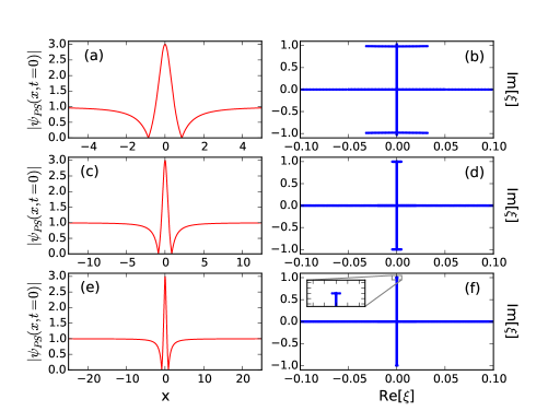
Figure 2: Spatial profiles (left) and corresponding spectral portraits (right) of the PS given by Eq. (11). The spectral portraits have been computed with numerical boxes having sizes $L=10$ (b); $L=25$ (d) and $L=50$ (f).

Even though the IST spectrum of the PS is slightly corrupted by the truncation procedure, the computed spectral portraits preserve the global information that the analyzed structure is the PS. First, the computed spectra are composed of three bands, which means that the analyzed structure is a genus $2$ solution of Eq. (1). Then, the computed IST spectra have a symmetry with respect to the vertical imaginary axis that is reminiscent of the degenerate nature of the analyzed structure. Finally, the endpoints delimiting the three computed bands are close to the correct theoretical positions $\pm i$ in the complex plane.

If the truncation of the PS can be simply understood as a local procedure dedicaded to isolate its central core part, the subsequent IST analysis made by using BO’s method or the Fourier collocation method must be understood as representing the numerical IST analysis of the truncated PS of size $L$ that has been expanded to produce a periodic pattern of period $L$. The BO method indeed provides the IST spectra of potentials that are periodic in space. In this method, the period of the analyzed structure is naturally equal to the size $L$ of the numerical box and the period $L$ is inherently encoded into the trace $\Delta$ of the transfer matrix. It is therefore implicit in BO’s method that the IST analysis of a periodic structure of period $L$ is made. On the other hand, in the Fourier collocation method extensively used in ref. Randoux et al. (2016b), the periodization of the truncated PS must be made in an explicit way prior to the IST analysis. As discussed in detail in ref. Randoux et al. (2016b), it is mandatory to produce a periodic series of truncated PS before solving the ZS problem in Fourier space. Our computations show that, as long as the analysis reported in Fig. 2 is concerned, there is no significant quantitative difference between numerical results obtained with the Fourier collocation method and with the BO method.

Summarizing, the numerical IST analysis described in this Section represents a tool which has been used here to perform a local finite-band approximation of the PS defined by Eq. (11). This tools captures the fact that the PS truncated to its central core part is locally composed of three dominant nonlinear modes that are embedded within some symmetric interaction process.

III Nonlinear spectral analysis of the Peregrine soliton observed in optical fiber experiments

In the experiment reported in ref. Kibler et al. (2010), a weakly modulated light wave is injected inside an optical fiber. Nonlinear propagation inside the fiber leads to the generation of a breather structure that exhibits properties of localization in space and time close to the PS. The experimental conditions and the physical parameters characterizing this optical fiber experiment are known with a very good accuracy. Some important insight into the understanding of the experimental results reported in ref. Kibler et al. (2010) can first be recalled by means of numerical simulations. In Sec. III.1, we report numerical simulations in which we analyze in detail the optical fiber experiment reported in ref. Kibler et al. (2010). In Sec. III.2, we perform the nonlinear spectral analysis of the optical signal that has been recorded in ref. Kibler et al. (2010).

III.1 The optical fiber experiment analyzed by numerical simulations

As underlined in ref. Kibler et al. (2010), the PS represents an ideal asymptotic limit that can never be reached in practice. In these circumstances, the approach that was taken in ref. Kibler et al. (2010) has consisted in demonstrating that the spatiotemporal localization properties of the PS are however experimentally observable. In the optical fiber experiment reported in ref. Kibler et al. (2010), SFBs have been generated by weakly modulating the plane wave used as an initial condition. Shifting the frequency of the pertubative Fourier component added to the plane wave while appropriately adjusting the optical power, it has been shown that the breather structures emerging at the nonlinear stage of the development of modulational instability exhibit properties of localization in space and time that are compatible with the ones characterizing the PS, see Fig. 2(b) of ref. Kibler et al. (2010). At the point where the strongest localization effects occur in the optical fiber experiment ($a=0.42$ in Fig. 5(d) of ref. Kibler et al. (2010)), the intensity profile of the experimentally observed localized structure has a core part that fits quantitatively very well the profile characterizing the PS mathematically defined by Eq. (11).

Before using the numerical implementation of the periodic IST for the analysis of the experiment reported in ref. Kibler et al. (2010), one important comment should be made about the suitability of this mathematical tool for the analysis of the data recorded in optical fiber experiments that take periodic signals as initial condition Kibler et al. (2010, 2012); Hammani et al. (2011a); Frisquet et al. (2013, 2014). The fact that the initial condition is generated by Fourier synthesis in a number of optical fiber experiments has the important consequence that it is breather structures having some periodicity both in space and time that are inherently produced in all these experiments. In these circumstances, periodic IST naturally represents the appropriate tool for the nonlinear analysis of the observed coherent structures.

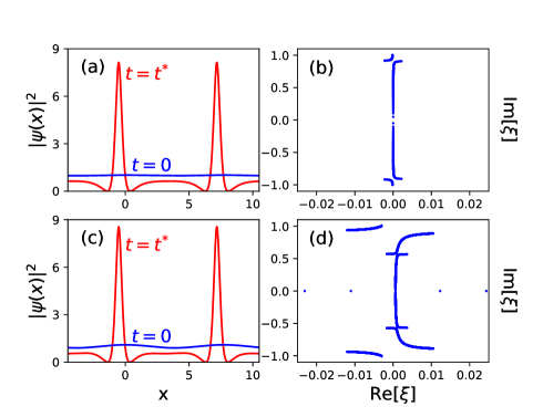
Figure 3: Numerical simulations of Eq. (1) (left column) and the corresponding IST spectra (right column) computed with the initial condition given by Eq. (12). Parameters are (a) (b) $\epsilon=0.01$, $k_{0}=0.822$, (c), (d) $\epsilon=0.05$, $k_{0}=0.822$. $t^{*}$ represent the times at which the breather structures reach their maximum intensities: (a) $t^{*}=3.162$, (c) $t^{*}=2.117$. The size $L=7.64$ of the box used for numerical IST analysis is equal to the period of the modulated wave ($L=2\pi/k_{0}$).

Taking the 1D-NLSE in the form given by Eq. (1), the field used as initial condition in the experiment of ref. Kibler et al. (2010) reads

$$\psi(x,t=0)=\psi_{0}(x)=1+\epsilon\,\,e^{-ik_{0}x}$$ (12)

with $k_{0}=2\pi/L$ where $L$ represents the size of the box that will be used here for the numerical IST analysis. The dimensionless spatial frequency $k_{0}$ is directly related to the frequency detuning between the two lasers used in the experiment and it also depends on the nonlinear length and on the second-order dispersion coefficient of the fiber, see Appendix A for details about relations between physical parameters and dimensionless parameters. In the experiments reporting the so-called maximally compressed pulse (see Fig. 5(d) of ref. Kibler et al. (2010)) that is well fitted by Eq. (11), the numerical values of $k_{0}$ and $\epsilon$ are $0.822$ and $0.225$, respectively.

Fig. 3(a) shows the intensity profile $\psi(x,t^{*})$ of the breather structure that is obtained from numerical integration of Eq. (1) by taking the value $k_{0}=0.822$ typifying the experiment. On the other hand, the numerical value of the parameter $\epsilon$ is $0.01$, which is much smaller that the experimental value of $0.225$. With these parameters, the time at which the structure reaches its maximum amplitude is $t^{*}=3.162$ which corresponds to a virtual propagation distance of $\sim 2.1$ km in an optical fiber with no losses and with linear and nonlinear parameters identical to those typifying the fiber used in ref. Kibler et al. (2010), see Appendix A.

Fig. 3(b) shows the IST spectral portrait of the breather structure shown in Fig. 3(a). It has been computed by using the Fourier collocation method but identical numerical results are obtained by using BO’s method. Let us emphasize that the spectral portrait is time-independent: identical IST spectra are obtained by taking the field at $t=0$, at $t=t^{*}$ or at any other evolution time. The spectral portrait of Fig. 3(b) being composed of three bands, the IST spectral analysis reveals that the generated structure represents a genus $2$ solution of the 1D-NLSE that can be closely related to the AB.

The spatially periodic breather structures shown in Fig. 3(a,b) indeed bear strong resemblance to the ABs, which are typically associated with the development of modulational instability of the plane wave modified by a small-amplitude periodic perturbation Dudley et al. (2009); Hammani et al. (2011a); Mussot et al. (2018). In this connection let us emphasize that the AB solution represents a pure space-periodic homoclinic solution of the 1D-NLSE that breathes only once in time. As illustrated in Fig. 1(a) of ref. Ablowitz et al. (2001), the IST spectrum of the pure AB is very particular because it is composed of a branchcut between $+i$ and $-i$ and also of two double points lying at positions given by $\pm i\,\sqrt{2a}$, with the conventions of ref. Kibler et al. (2010). As discussed in detail in ref. Ablowitz et al. (1996, 2001), the modulation of a plane wave by two weak side bands generally produces more complex solutions than the pure AB. However, the spectra of the structures generated by periodic modulation of the plane wave retain some proximity to the pure AB solution.

Here, by modulating the plane wave with only one side band, two gaps are opened in the branch cut crossing the real axis, see Fig. 3(b). The central position of these gaps are $\pm i\,0.914$ which is very close to the theoretical value $\pm i\,\sqrt{2a}=\pm i\,0.916$ that characterizes the pure AB solution ($a=0.42$) considered in ref. Kibler et al. (2010). The IST spectrum is not symmetric with respect to the vertical imaginary axis because the Fourier spectrum of the initial condition is itself not symmetric. This initial asymmetry induces a slight drift of the structure that moves in the $(x,t)$ plane with a non-zero velocity. This drift in the $(x,t)$ plane is readily observable in Fig. 3(a) where the breather structure reaches its peak intensity at $(x=-0.51,t^{*})$ while the initial field intensity is maximal at $(x=0,t=0)$. Such a breather structure was classified as a “left” state in ref. Ablowitz et al. (1996, 2001), i. e. a left-travelling wave solution of the 1D-NLSE. In ref. Zakharov and Gelash (2013); Kibler et al. (2015); Akhmediev et al. (2009a) it was also considered into the class of the general one-breather solution with an arbitrary group velocity [26,27,39]. The impact of an asymetric initial excitation of ABs has been analyzed in Refs. Frisquet et al. (2013); Akhmediev et al. (2009d); Kibler (2017). We note that exact analytical description of the formation of ABs and related structures in the initial value problem (1), (12) was also developed in the recent work Grinevich and Santini (2017) using the finite-gap theory.

Increasing the value of $\epsilon$ to $0.05$ while keeping the same value $k_{0}=0.822$ for the wavenumber characterizing the small perturbation of the plane wave, numerical simulations of Eq. (1) reveal that the breather structure shown in Fig. 3(c) now reaches its maximum amplitude at $t^{*}=2.117$. Even though the intensity profile of the breather structure obtained for $\epsilon=0.05$ is similar to the one of the breather structure obtained for $\epsilon=0.01$, the spectral portrait reveals that the analyzed structure is no longer a genus $2$ solution of the 1D-NLSE but a genus $4$ solution, i.e. the solution involving $g+1=5$ nonlinear “eigenmodes” Tracy et al. (1984); Randoux et al. (2016a). In terms of the IST spectrum, two additional gaps are now open in the vertical band crossing the real axis, which results in a IST spectrum now composed of $5$ bands. This change in the genus of the solution implies that some more complex spatiotemporel evolutions can possibly be observed, as shown e.g. in refs. Ablowitz et al. (1996) and Bertola et al. (2016). Such observations are also known to be related to the phenomenon of higher modulation instability recently observed in optics and in hydrodynamics Hammani et al. (2011b); Erkintalo et al. (2011); Kimmoun et al. (2017); Kibler (2017), wherein non-ideal excitation of first-order breathers (ABs, PS…) or propagation losses were identified as perturbations that introduce deviations from the expected nonlinear dynamics on longer propagation distances (simply due the unstable nature of NLS breathers). In particular, it was shown that higher order modulation instability arises from perturbations on breathers close to the PS limit, thus resulting in a nonlinear superposition (i.e., complex arrangement) of several elementary breathers.

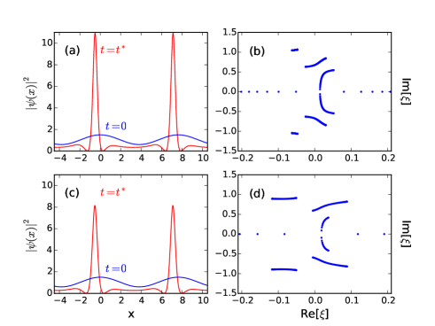
Figure 4: (a) Numerical simulations of Eq. (1) with the initial condition given by Eq. (12) ($\epsilon=0.225$, $k_{0}=0.822$) and (b) corresponding IST spectrum. (c) Numerical simulations of Eq. (13) with the initial condition given by Eq. (12). (d) IST spectrum of the coherent structure $\psi(x,t^{*})$ plotted with red lines in (c). The numerical values of the parameters correspond the optical fiber experiment reported in ref. Kibler et al. (2010) and their numerical values are $\epsilon=0.225$, $k_{0}=0.822$, $\kappa=0.076$. $t^{*}$ represent the times at which the breather structures reach their maximum intensities: (a) $t^{*}=1.192$, (c) $t^{*}=1.273$. The size $L=7.64$ of the box used for numerical IST analysis is equal to the period of the modulated wave ($L=2\pi/k_{0}$).

Fig. 4(a) shows the result of the numerical simulation of Eq. (1) for a value of $\epsilon=0.225$ identical the one typifying the optical fiber experiment reported in ref. Kibler et al. (2010). Fig. 4(b) represents the corresponding IST spectrum that displays five well-separated bands. This shows that the generated structure remains a genus $4$ solution of the 1D-NLSE when the value of $\epsilon$ is increased from $0.05$ to $0.225$. The peak intensity of the generated breather structure reaches a value $\sim 11$ at the time $t^{*}=1.192$. This value is greater than the peak intensity of $9$ that can be reached by the PS but it should be kept in mind that fiber losses have not yet been taken into account in the numerical simulation.

For a better quantitative description of the experiment reported in ref. Kibler et al. (2010), fiber losses should be taken into account. To describe their influence, a linear damping term must be added to Eq. (1) that becomes

$$i\psi_{t}+\psi_{xx}+2\,|\psi|^{2}\,\psi+i\,\kappa\,\psi=0.$$ (13)

$\kappa\in\mathbb{R}^{+}$ is a damping parameter that depends on the fiber attenuation coefficient, see Appendix A for the correspondance between physical parameters and dimensionless parameters. Fig. 4(c) shows the result of the numerical simulation of Eq. (13) with the parameters $\epsilon=0.225$, $k_{0}=0.822$, $\kappa=0.076$ that characterize the optical fiber experiment reported in ref. Kibler et al. (2010). Now that the effect of dissipation is taken into account, numerical simulations of the experiment show that the maximum peak intensity reached by the breather structure is $\sim 8.2$ at time $t^{*}=1.273$. Moreover the core part of the intensity profile of the structure numerically obtained can be well fitted by Eq. (11), like in ref. Kibler et al. (2010).

Now that dissipation is included in the 1D-NLSE, the wave system can no longer be considered as being described by an integrable equation. Rigorously speaking, the IST tools described in Sec. II.1 can no longer be used to analyze the generated structures. However, it should be emphasized that dissipation is weak enough in the experiment ($\kappa=0.073$) to be considered as a small perturbative effect. In these circumstances, the fact that the optical power slightly decays all along the optical fiber induces some slow modulation of the coherent structure. If the IST analysis of the generated structure is made locally in time (i.e. after some propagation distance inside the fiber) in the presence of dissipation, we observe a gradual deformation of the spectral bands. At a time $t\sim 0$, the numerically computed spectrum is very close to the one shown in Fig. 4(b) but at time $t^{*}=1.273$, the spectral deformation is no longer negligible, see Fig. 4(d). Dissipative effects break the integrability of the wave equation, and the isospectrally condition (i. e. time-independence of the IST spectrum) can no longer be satisfied in these circumstances. However, it must be emphasized that dissipative effects remain of perturbative nature and that their presence does not corrupt the qualitative structure of the IST spectrum in the sense that it is still composed of five bands.

In conclusion, the numerical IST analysis of the experiment reported in ref. Kibler et al. (2010) reveals that the initial condition used in the experiment exhibits $5$ spectral bands, i.e. can be more accurately approximated by a genus $4$ solution of the 1D-NLSE at $t=0$, i.e. at the input end of the fiber. Weak dissipative effects occurring inside the optical fiber play a perturbative role and produce a slow variation of the intensity profile and, therefore, of the spectral characteristics of the generated solution. From the perspective of nonlinear spectral analysis, the observed breather structure, therefore, represents a slowly modulated genus $4$ solution of the 1D-NLSE with the modulation of spectral characteristics occurring due to weak dissipative effects.

III.2 Nonlinear spectral analysis of the experimental data

In the optical fiber experiment reported in ref. Kibler et al. (2010), the intensity and the phase of the optical signal have been measured over several periods by using the so-called Frequency Resolved Optical Gating (FROG) technique. The experimentally recorded signals rescaled to dimensionless variables are plotted in red lines in Fig. 5(a) and 5(b), see Appendix A for the correspondance between physical variables and dimensionless variables. The blue lines in Fig. 5(a) and 5(b) represent the intensity profile $|\psi(x)|^{2}=|\psi(x,t^{*})|^{2}$ and the phase profile $\phi(x)=\phi(x,t^{*})$ of the breather structure ($\psi(x)=|\psi(x)|e^{i\phi(x)}$) computed from numerical simulations of Eq. (13) with the dimensionless parameters that characterize the optical fiber experiment, i. e. the function $|\psi(x)|^{2}$ plotted with blue lines in Fig. 5(b) is identical to the function $|\psi(x,t^{*})|^{2}$ plotted in Fig. 4(c).

Similar to ref. Kibler et al. (2010), Fig. 5(b) shows that there is a very good quantitative agreement between the intensity profile that has been experimentally recorded and the intensity profile that is computed from numerical integration of Eq. (13). However, the careful analysis of experimental data recorded in ref. Kibler et al. (2010) reveals that the SFB structure that is generated in the experiment present phase and intensity profiles that are slowly modulated not only by fiber losses but also by pertubative third-order dispersive effects occurring inside the optical fiber. Indeed, the phase profile of SFB experimentally recorded exhibits a marked asymmetry in the the region surrounding the soliton core part of the observed SFB. A phase jump of $\sim-\pi$ measured on the left-hand side of the coherent structure is followed by another phase jump is of $\sim-\pi$ on the right-hand side of the coherent structure. Such a pronounced asymmetry is not found in the numerical simulation of Eq. (13) that reveals a nearly symmetric phase profile with a phase jump of $\sim+\pi$ followed by another phase jump of $\sim-\pi$, see blue line in Fig. 5(a). The asymmetry of the phase profile experimentally observed arises from the occurrence of perturbative third-order dispersion terms that are not included in Eq. (13). Inclusion of the third-order dispersion term in numerical simulations reproduces quantitatively well the asymmetry of the phase profile experimentally observed without significantly modifying the intensity profile computed from numerical integration of Eq. (13). This asymmetry in the phase jump simply arises from the fact that one side of the breather has passed the maximal focusing point before the other side (i.e., the phase tips over $+\pi\leftrightarrow-\pi$) .

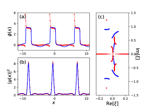
Figure 5: (a) Phase profile (red line) and (b) intensity profile (red line) recorded in the optical fiber experiment reported in ref. Kibler et al. (2010). The phase and intensity profiles plotted with blue lines in (a) and (b) are computed from the numerical simulation of Eq. (13) with parameters of the experiment ($\epsilon=0.225$, $k_{0}=0.822$, $\kappa=0.076$). (c) Spectral portraits computed from the optical signals recorded in the experiment (red dots) and from numerical simulations of Eq. (13) (blue dots).

Fig. 5(c) shows the result of the nonlinear spectral analysis of the experiment reported in ref. Kibler et al. (2010). The spectrum plotted in red dots is the spectrum of the optical signal that has been experimentally recorded in ref. Kibler et al. (2010). The spectrum plotted in blue dots is the spectrum of the coherent structure $\psi(x,t^{*})$ computed from numerical simulation of Eq. (13) with the parameters of the experiments, i. e. the spectrum in blue dots in Fig. 5(c) is identical to the spectrum in Fig. 4(d). Due to third-order dispersion, the phase profiles are different in the experiment and in the numerical simulation of Eq. (13). Therefore the two spectral portraits in Fig. 4(c) are not identical. However, the nonlinear spectral analysis of the experimental data reveals that the SFB structure observed in the optical fiber experiment has a spectrum composed of five bands which means that the observed SFB structure has to be classified as a genus $4$ solution of the 1D-NLSE.

In conclusion, the nonlinear spectral analysis of experimental data reported in ref. Kibler et al. (2010) shows that the observed structure can be more accurately described by a genus $4$ solution of the 1D-NLSE having a spectral portrait composed of $5$ bands. Even though this solution has a mathematical nature that is different from the PS’s one (a degenerate genus 2 solution of the 1D-NLSE), the SFB locally observed in optical fiber experiments retains some degree of proximity to the PS in the sense that it has similar properties of localization in space and time. The detailed nonlinear spectral analysis also reveals that weak dissipative effects and third-order dispersive effects occurring inside the optical fiber play some perturbative roles by producing a slow modulation (with propagation distance) of the spectral characteristics of the observed SFB.

IV Nonlinear spectral analysis of the Peregrine soliton observed in water tank experiments

In the hydrodynamic experiment reported in ref. Chabchoub et al. (2011), a breather structure is generated from the motion of a flap inside a $15$ m $\times$ $1.6$ m $\times$ $1.5$ m water wave tank with $1$ m water depth. The flap displacement was chosen to be proportional to the amplitude of the PS to be generated, i.e the flap motion is set to be directly proportional to the water surface elevation that is determined from Eq. (11). The generation of the initial condition is made by chosing a time $t_{0}<0$ in Eq. (11) in such a way that the generated breather reaches its maximum amplitude near the end of the water tank.

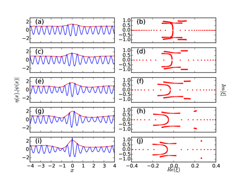
Figure 6: Nonlinear spectral analysis of the experimental data recorded in the hydrodynamic experiment reported in ref. Chabchoub et al. (2011). Left column: water elevation $\eta(x,t^{*})$ (blue lines) and modulus $|\psi(x,t^{*})|$ (red lines) of the complex envelope of the wave packets. The evolution times $t^{*}$ and corresponding propagation distances $D$ inside the water tank are (a) $t^{*}=7.8\times 10^{-3}$, $D=0.1$ m, (c) $t^{*}=0.1573$, $D=2.1$ m, (e) $t^{*}=0.3146$, $D=4.1$ m, (g) $t^{*}=0.4719$, $D=6.1$ m, (i) $t^{*}=0.629$, $D=8.1$ m. Right column: spectral portraits of the experimental signals. Computation of the spectral portraits is made with a numerical box having a size $L=8$.

In the experiment reported in ref. Chabchoub et al. (2011), the water waves that propagate inside the tank are progressive Stokes waves having their complex envelopes $\psi$ that are slowly modulated in space and time. The water elevation $\eta$ is the real variable that is measured at several localized points inside the water tank, see Fig. 3 of ref. Chabchoub et al. (2011) or left column of Fig. 6. As discussed in detail, e.g. in ref. Osborne (2010), the complex envelope $\psi$ can be constructed from the measurement of the free surface elevation $\eta$ by using the Hilbert transform.

In our analysis of the hydrodynamic data recorded in ref. Chabchoub et al. (2011), the signals recorded by several capacitance gauges are first rescaled to dimensionless form, see Appendix B for the correspondance between physical variables and dimensionless variables. Then, the Hilbert transform is used to determine the complex envelope $\psi(x,t^{*})$ of the wave at different times $t^{*}$ that correspond to the different positions of the gauges inside the water tank. The normalized surface elevation $\eta(x,t^{*})$ and the corresponding envelope $|\psi(x,t^{*})|$ obtained by using this procedure are plotted in the left column of Fig. 6.

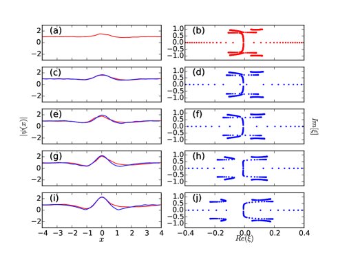
Figure 7: Left column: Numerical simulations of Eq. (13) while taking the signal measured by the first gauge (red line in (a)) as initial condition. The red lines represent experimental signals and the blue lines represent the results of the numerical simulation of Eq. (13) with $\kappa=1.6\times 10^{-2}$. The evolution times $t^{*}$ and the corresponding propagation distances $D$ inside the water tank are the same as in Fig. 6, i.e. (a) $t^{*}=7.8\times 10^{-3}$, $D=0.1$ m, (c) $t^{*}=0.1573$, $D=2.1$ m, (e) $t^{*}=0.3146$, $D=4.1$ m, (g) $t^{*}=0.4719$, $D=6.1$ m, (i) $t^{*}=0.629$, $D=8.1$ m. Right column: spectral portraits of the signals computed from numerical simulation of Eq. (13). Computation of the spectral portraits is made with a numerical box having a size $L=8$.

Contrary to the optical fiber experiment discussed in detail in Sec. III, the hydrodynamic experiment reported in ref. Chabchoub et al. (2011) presents the advantage that the buildup of the breather structure can be observed and measured. Nonlinear spectral analysis of the experimental signals plotted in Fig. 6 reveals that the observed structure represents a genus $4$ solution of the 1D-NLSE having its spectral properties that are slowly modulated in time, see right column in Fig. 6. The spectrum at the initial time (i.e. near the wavemaker) is composed of five bands and it is relatively confined around the vertical imaginary axis. It is remarkable to observe that the nonlinear spectral analysis evidences a slow gradual deformation of the five spectral bands with time (i. e. with propagation distance along the water tank). Fig. 6 indeed shows that the spectrum is not time-independent but that it slowly spreads along the real axis. Similar spectral behavior has been evidenced in Sec. III.1 where dissipation has been shown to induce qualitatively the same kind of spectral effect, cf. Fig. 4(b) and 4(d).

These results suggest to conduct numerical simulations of Eq. (13) to investigate the influence of dissipation on the shape of the spectral portraits. We have made numerical simulations of Eq. (13) by taking an initial condition that is given by the signal recorded by the first capacitance gauge located only $10$ cm away from the wavemaker. The numerical value of the damping parameter $\kappa=1.6\times 10^{-2}$ has been determined from the measurement of the attenuation of the signals recorded by all the other capacitance gauges, see Appendix B. Taking the signal recorded by the first gauge as initial condition for the integration of Eq. (13), the modulus of $\psi$ that is computed from the numerical simulation is in good quantitative agreement with the envelope of the experimental signals, see left column in Fig. 7. Only a slight asymmetry measured in the experiment is not found at long evolution time (i.e. far from the wavemaker) in the numerical simulation of Eq. (13), see Fig. 7(g)(i).

Performing the nonlinear spectral analysis of the function $\psi(x,t^{*})$ computed from numerical simulations at evolution times $t^{*}$ corresponding to discrete positions at which the signals have been recorded in the experiment, we observe a spreading of the spectral portrait around the vertical imaginary axis that has already been evidenced in Fig. 6 in the nonlinear spectral analysis of the experimental data. This slow modulation of the spectral characteristics of the analyzed structure shows that dissipation plays a measurable role in the experiment reported in ref. Chabchoub et al. (2011). Note that recent works have shown that dissipation plays a significant influence in the buildup dynamics of breather solutions of the 1D-NLSE Kimmoun et al. (2016, 2017).

Note that there is a reasonably good quantitative agreement between spectral portaits plotted in Fig. 6(d)(f) and in Fig. 7(d)(f). This shows that the dynamics of the wavepacket is correctly described by Eq. (13) until $t^{*}=0.314$ (i.e. until the wave packet reaches the gauge that is located $5.10$ m away from the wavemaker). Beyond this evolution time, the spectra computed from the analysis of the experimental data and from the numerical simulation of Eq. (13) become of qualitatively different natures, compare Fig. 6(h)(j) and Fig. 7(h)(j). This means that wave propagation is not ruled by Eq. (13) for evolution times greater than $0.314$ (i.e. for propagation distances greater than $5.10$ m). Nonlinear spectral analysis thus reveals that higher order effects play some non-negligible role in the buildup dynamics of the breather structure for the chosen carrier parameters that has a significant steepness of $0.1163$. With this value of the steepness, higher-order effects are to be expected given the significant focusing of the wave field Shemer et al. (2002); Islas and Schober (2011). Note that their contribution can be reduced, when choosing smaller carrier steepness values in accordance with weakly nonlinear theory Chabchoub et al. (2012c).

V Discussion and Conclusion

In this paper, we have analyzed the data recorded in an optical fiber experiment Kibler et al. (2010) and in a hydrodynamic experiment Chabchoub et al. (2011) that have reported the observation of SFB having properties of localization in space and time similar to those of the PS. Our approach is based on the integrable nature of the 1D-NLSE that governs at leading order the propagation of the optical and hydrodynamical waves in these two experiments. Solving the ZS spatial problem with periodic boundary conditions by using Floquet spectral theory, we have computed the spectral (IST) portraits of the PSs observed in the two experiments, thus obtaining their nonlinear spectral signature.

Contrary to linear (Fourier) spectral analysis that mostly provides spectra having some universal triangular shape whatever the exact nature of the SFB under consideration Kibler et al. (2010); Frisquet et al. (2013, 2014); Kibler et al. (2015); Akhmediev et al. (2011a), we obtain spectral signatures having some shapes that strongly depend on the exact phase and intensity profiles of the examined SFB. These spectral portraits can be interpreted within the framework of the so-called finite gap theory (or periodic IST). In particular, the number $g+1$ of bands composing the nonlinear spectrum determines the genus $g$ of the solution that parametrizes the complexity of the space-time evolution of the considered solution. Note that phase portraits recently used e. g. in ref. Kimmoun et al. (2016); Mussot et al. (2018) provide some other useful geometric representation of the dynamics of breather solutions of the 1D-NLSE.

The nonlinear spectral analysis of the SFB observed both in the optical fiber experiment and in the water tank experiment reveals that they represent general genus $4$ solutions of the 1D-NLSE that may exhibit a space-time evolution that is much more complex than a simpler degenerate genus $2$ solution like PS or ABs, as shown in the recent experiments reported in ref. Hammani et al. (2011b); Erkintalo et al. (2011); Kibler (2017). Moreover, nonlinear spectral analysis reveals that the spectrum of the observed SFB slowly changes with the propagation distance, thus confirming a clear evidence of the influence of perturbative higher order effects like dissipation in the experiments Kimmoun et al. (2016, 2017).

As discussed in detail in ref. Islas and Schober (2005); Calini and Schober (2012), the size of the gaps between the endpoints of the spectral branches determines the proximity to some homoclinic solutions of the 1D-NLSE. The smaller is the size of these gaps, the closer is the observed solution to some homoclinic solution associated with some high peak intensity. An appropriate (and non trivial) choice of the initial phases of the finite-gap solution would permit to reduce the size of the gaps, thus approaching homoclinic solutions.

From a more practical perspective, nonlinear spectral analysis could possibly be used as a predictive tool for the prediction of the space-time evolution of coherent (soliton- or breather-like) structures emerging in random wave systems ruled by integrable equations Walczak et al. (2015); Akhmediev et al. (2011b); Cousins and Sapsis (2016). The measurement of the size of the spectral bands provides some information about the maximum amplitude that can be possibly reached by the coherent structure under consideration. As discussed in ref. Islas and Schober (2005); Calini and Schober (2012), the measurement of the size of the spectral gaps indicates the proximity to homoclinic orbits and is therefore related to the probability of emergence of a rogue wave.

Appendix A Relation between physical variables and dimensionless variables in the optical fiber experiment

In the optical fiber experiment reported in ref. Kibler et al. (2010), light propagation is governed by the dimensional 1D-NLSE

$$i\frac{\partial A}{\partial z}-\frac{\beta_{2}}{2}\frac{\partial^{2}A}{\partial T^{2}}+\gamma|A|^{2}A+i\frac{\alpha}{2}A=0$$ (14)

where third-order dispersion effects are not taken into account. $A(z,T)$ is the slowly-varying complex envelope of the electric field propagating inside the core of the single-mode fiber. $z$ represents the longitudinal coordinate measuring the propagation distance along the fiber and $T$ is the time measured in the retarded frame moving with light pulses. $\beta_{2}$ and $\gamma$ represent the second-order dispersion coefficient and the Kerr coefficient of the optical fiber, respectively. For the fiber that was used in ref. Kibler et al. (2010), these parameters are $\beta_{2}=-8.85\,\times\,10^{-28}$ s² m^-1 and $\gamma=0.01$ W^-1 m^-1. $\alpha$ is the fiber power attenuation coefficient that is equal to $2.3\,\times\,10^{-4}$ m^-1 ($\alpha=1$ dB/km).

Considering that the optical input power is $P_{0}$, the normalized optical field is defined by $\psi=A/\sqrt{P_{0}}$. Taking a definition commonly adopted in nonlinear fiber optics, the nonlinear length is given by $L_{NL}=1/(\gamma P_{0})$. In the optical fiber experiment of ref. Kibler et al. (2010), the input power $P_{0}$ is $300$ mW and the nonlinear length is of $333$ m. Introducing the dimensionless time and space variables $t=2\gamma P_{0}\,z$ and $x=\sqrt{\gamma P_{0}/|\beta_{2}|}\,T$ together with the damping parameter $\kappa=\alpha/(\gamma P_{0})$, Eq. (14) takes the following dimensionless form

$$i\psi_{t}+\psi_{xx}+2\,|\psi|^{2}\,\psi+i\,\kappa\,\psi=0.$$ (15)

In the optical fiber experiment of ref. Kibler et al. (2010), the damping parameter is $\kappa=7.6\times 10^{-2}$.

The spatial frequency $k_{0}$ of the dimensionless modulated field that is used as initial condition (see Eq. (12)) is given by

$$k_{0}=2\pi\Delta f\sqrt{\frac{|\beta_{2}|}{\gamma P_{0}}}$$ (16)

where $\Delta f=241$ GHz is the frequency detuning between the two lasers used in the experiment. With the numerical values of the physical parameters used in the experiment, the numerical value of $k_{0}$ is $0.822$.

Appendix B Relation between physical variables and dimensionless variables in the hydrodynamic experiment

In the hydrodynamic experiment reported in ref. Kibler et al. (2010), the evolution of the one-dimensional deep-water packets can be described by the following equation Kimmoun et al. (2016):

$$i\left(\frac{\partial a}{\partial z}+\frac{1}{c_{g}}\frac{\partial a}{\partial\tau}\right)-\frac{1}{g}\frac{\partial^{2}a}{\partial\tau^{2}}-k_{0}^{3}|a|^{2}a=i\Gamma a.$$ (17)

$\tau$ and $z$ represent the time and the longitudinal coordinate measuring the propagation distance alond the 1D-flume, respectively. $g$ denotes the gravitational acceleration and $k_{0}$ is the wave number. $k_{0}$ is linked to the pulsation $\omega_{0}$ of the carrier wave by the dispersion relation of the linear deep water wave theory $\omega_{0}=\sqrt{g\,k_{0}}$. $c_{g}=\frac{\omega_{0}}{2k_{0}}$ represents the group velocity of the wave packets. The surface elevation $\eta(z,\tau)$ of water is given by $\eta(z,\tau)=\Re(a(z,\tau)\exp[i(k_{0}z-\omega_{0}t)])$. $\Gamma$ represents the dissipation rate. Introducing the amplitude of the carrier wave $a_{0}$, the steepness is defined by $\epsilon=a_{0}k_{0}$.

Introducing the dimensionless time and space variables $t=-\frac{1}{2}a_{0}^{2}k_{0}^{3}z$ and $x=\frac{\sqrt{2}a_{0}k_{0}\omega_{0}}{2}\left(\tau-\frac{z}{c_{g}}\right)$ together with the normalized complex envelope of the elevation field $\psi=a/a_{0}$, Eq. (17) becomes

$$i\psi_{t}+\psi_{xx}+2\,|\psi|^{2}\,\psi+i\,\kappa\,\psi=0$$ (18)

where $\kappa=\frac{2\Gamma}{a_{0}^{2}k_{0}^{3}}$. In the hydrodynamic experiment reported in ref. Chabchoub et al. (2011), the numerical values of $a_{0}$, $k_{0}$, $\omega_{0}$ are $0.01$ m, $11.63$ m^-1, $10.7$ s^-1, respectively. The dissipation rate $\Gamma$ measured from experimental signals is $\Gamma=1.26\times 10^{-2}$ m^-1 and the value of the damping parameter is $\kappa=1.6\times 10^{-2}$.