Quasi-stable configurations of torus vortex knots and links

Abstract

The dynamics of torus vortex configurations $V_{n,p,q}$ in a superfluid liquid at zero temperature ($n$ is the number of quantum vortices, $p$ is the number of turns of each filament around the symmetry axis of the torus, and $q$ is the number of turns of the filament around its central circle; radii $R_{0}$ and $r_{0}$ of the torus at the initial instant are much larger than vortex core width $\xi$) has been simulated numerically based on a regularized Biot-Savart law. The lifetime of vortex systems till the instant of their substantial deformation has been calculated with a small step in parameter $B_{0}=r_{0}/R_{0}$ for various values of parameter $\Lambda=\log(R_{0}/\xi)$. It turns out that for certain values of $n$, $p$, and $q$, there exist quasi-stability regions in the plane of parameters $(B_{0},\Lambda)$, in which the vortices remain almost invariable during dozens and even hundreds of characteristic times.

I Introduction

Vortex knots and links have been objects of interest in the classical fluid dynamics since the 19-th century. In particular, Lord Kelvin Kelvin put forth the hypothesis that uniformly rotating and propagating (along a certain axis) symmetric stationary configurations of $n$ thin vortex filaments (each with circulation $\Gamma$) can exist in an ideal fluid. The shape of the filaments is close to torus vortices $V_{n,p,q}$ that are determined parametrically by the following expressions:

$$X_{j}(\beta) = \Big{[}R_{0}+r_{0}\sin\Big{(}q\beta+\frac{2\pi j}{np}-\Theta_{0}\Big{)}\Big{]}\cos(p\beta),$$ (1)

$$Y_{j}(\beta) = \Big{[}R_{0}+r_{0}\sin\Big{(}q\beta+\frac{2\pi j}{np}-\Theta_{0}\Big{)}\Big{]}\sin(p\beta),$$ (2)

$$Z_{j}(\beta) = r_{0}\cos\Big{(}q\beta+\frac{2\pi j}{np}-\Theta_{0}\Big{)}+Z_{0},$$ (3)

where $j=1,\dots,n$ is a vortex number, $n$ is the number of quantized vortex filaments, longitudinal parameter $\beta$ runs through the interval $0\leq\beta<2\pi$, and $\Theta_{0}$ and $Z_{0}$ are linear functions of time $t$. Natural numbers $p$ and $q$ must have no common multipliers. It can easily be seen that $p$ is the number of turns of each filament around the symmetry axis of the torus and $q$ is the number of turns around its central circle. If $p>1$ and $q>1$, each vortex filament is a torus knot ${\cal T}_{p,q}$. If at least one of these numbers ($p$ or $q$) is equal to unity, each line is an unknot, ${\cal U}_{p,1}$ or ${\cal U}_{1,q}$, but it is linked in this case with all remaining lines (for $n\geq 2$). If $p=1$ and $q=1$, we obtain a link of $n$ rings.

Despite such a long history of the problem, such vortex knots and links have been produced experimentally for the first time quite recently KI2013 .

It should be noted that real objects closest to the theory are quantized vortex filaments in superfluid liquids (e.g., helium at a low temperature, for which the effect of the normal component is negligibly small). In this case, $\Gamma=2\pi\hbar/m_{\rm at}$ is the velocity circulation quantum ($m_{\rm at}$ is the mass of the helium atom), and the width of the core of each vortex is $\xi$. Unfortunately, the experimental technique for producing knots and links for quantum vortices has not been developed as yet.

It should be observed that exact stationary configurations of the torus type have not been found (even numerically) as yet, and their stability has not been tested. The difficulties are associated to a considerable extent with the fact that the steady-state solutions correspond not to the energy functional minimum for preset values of the momentum and angular momentum, but only to a saddle point. Therefore, we have to operate with approximate formulas (1)–(3). In a number of publications, the dynamics of torus vortices was simulated numerically for a small number of sets of parameters and for not very long time intervals, during which vortices could propagate along $z$ axis by not more than a few dozen $R_{0}$ ($R_{0}$ and $r_{0}$ are the radii of the torus), and then the deformation of the filaments increased [3-11]. In the quantum-mechanical case, this led to reconnections. It may appear that such results indicate an (albeit relatively weak) instability of torus knots and links.

The actual situation is more complicated and interesting. In the author’s recent publication [12], it was shown for simplest knots ${\cal T}_{2,3}$ and ${\cal T}_{3,2}$ that in the space of parameters $B_{0}=r_{0}/R_{0}$ and $\Lambda=\log(R_{0}/\xi)$ ($\xi$ is the vortex core width), there exist quasi-stability regions that are gaps between fundamental parametric resonances of various types, where a knot remains almost unchanged on the average for many dozen and even hundreds of characteristic times, passing distances that are sometimes equal to thousands of initial radii $R_{0}$. In other words, the toric shape of a vortex contains perturbation modes relative to the corresponding (unknown) stationary configuration, and the amplitudes of these modes increase with time in not all cases.

To determine quasi-stable regions, computer calculations of the lifetime of knots till the instant of their significant deformation with a small step in parameter $B_{0}$ for a preset value of $\Lambda$ were required. All quasi-stable zones of a trefoil knot ${\cal T}_{2,3}$ determined in [12] have a small width $\Delta B_{0}\lesssim 0.01$ and correspond to relatively “thin” tori with $B_{0}\lesssim 0.2$ (see the top panel in Fig. 1 below). It is significant that the maximal values of $B_{0}$ are attained for $\Lambda\approx 3.5$. For $\Lambda\lesssim 3$, such zones are absent, while for $\Lambda\gtrsim 6$, the zones are shifted to small $B_{0}\lesssim 0.1$. These regions have not been observed earlier in all probability precisely because of their “periphery” position and a small size.

A natural question arises: what is the situation with other knots and links? This study aims at the search for analogous quasi-stable configurations also for other $V_{n,p,q}$ apart from $V_{1,2,3}$ and $V_{1,3,2}$. It will be shown below that such configurations exist for not all sets $\{n,p,q\}$ (at least in the range of $B_{0}\gtrsim 0.1$ of interest; for small values of $n$, this range corresponds to considerable distances $l\sim 2r_{0}\gtrsim 4\xi$ between vortex cores for $\Lambda\approx 3$).

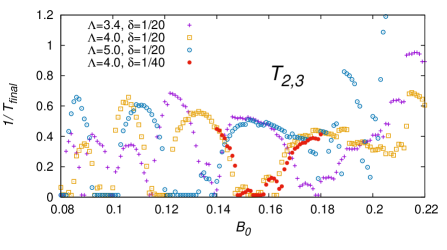
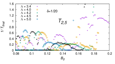
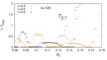
Figure 1: Reciprocal lifetime of vortex knots ${\cal T}_{2,q}$ for $q=3,5,7$ for different parameters $\Lambda$ and $B_{0}$. In all three panels, the quasi-stability zones in the form of segments close to the horizontal axis can be seen.

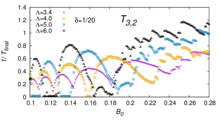
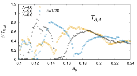
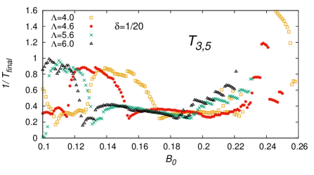
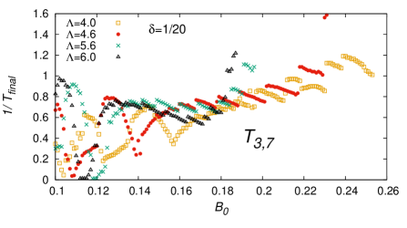
Figure 2: Reciprocal lifetime of vortex knots ${\cal T}_{3,q}$ for $q=2,4,5,7$. The quasi-stability zones are manifested most clearly for $q=2$ and $4$.

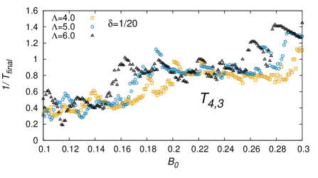
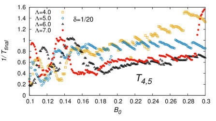
Figure 3: Reciprocal lifetime of vortex knots ${\cal T}_{4,3}$ and ${\cal T}_{4,5}$. The quasi-stability zones are absent.

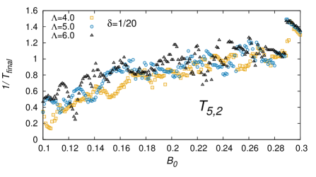
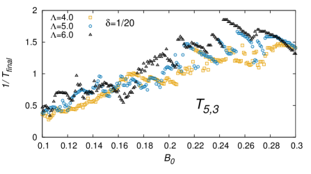
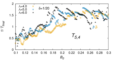
Figure 4: Reciprocal lifetime of vortex knots ${\cal T}_{5,q}$ for $q=2,3,4$. The quasi-stability zones are absent.

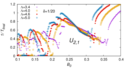
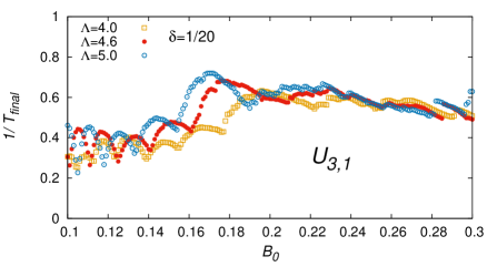
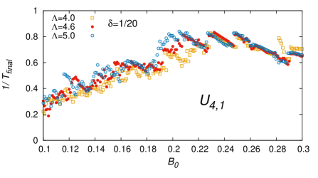
Figure 5: Reciprocal lifetime of vortex unknots ${\cal U}_{2,1}$, ${\cal U}_{3,1}$, and ${\cal U}_{4,1}$. For ${\cal U}_{2,1}$, quasi-stable configurations exist even for large $B_{0}\approx 0.2$.

II Dynamic model

Let us recall that the dynamics of several thin vortex filaments is governed to a high degree of accuracy by the regularized Biot-Savart law combined with the local induction contribution (see, for example, [13-15] and the vast literature cited therein),

$$\dot{\bf X}_{j}(\beta,t)=\sum_{i=1}^{n}\frac{\Gamma}{4\pi}\oint\frac{\tilde{\bf X}_{i}^{\prime}\times({\bf X}_{j}-\tilde{\bf X}_{i})}{\mbox{reg}_{\xi}|{\bf X}_{j}-\tilde{\bf X}_{i}|^{3}}d\tilde{\beta}+\frac{\Gamma\Lambda_{0}}{4\pi}\varkappa_{j}{\bf b}_{j},$$ (4)

where $\tilde{\bf X}_{i}={\bf X}_{i}(\tilde{\beta},t)$, $\tilde{\bf X}_{i}^{\prime}=\partial{\bf X}_{i}(\tilde{\beta},t)/\partial\tilde{\beta}$, $\Lambda_{0}$ is a dimensionless positive parameter of the order of unity, which characterizes the vortex core; $\varkappa_{j}$ is the local curvature of the $j$-th filament, and ${\bf b}_{j}$ is the local unit binormal vector. The method of regularization of logarithmically diverging integrals almost does not affect the dynamics of the filament if parameter $\Lambda_{0}$ is defined concordantly. For this purpose, the Rosenhead-Moore approximation is often used:

$$\mbox{reg}_{\xi}|{\bf X}_{2}-{\bf X}_{1}|^{3}=\sqrt{(|{\bf X}_{2}-{\bf X}_{1}|^{2}+\xi^{2})^{3}}.$$ (5)

Obviously, the dynamics of vortex filaments as 1D objects in the 3D space is invariant to arbitrary (regular) replacements of longitudinal parameter $\beta$. This fact makes it possible to supplement the right-hand sides of equations of motion (4) with terms of the form $\mu_{j}{\bf X}^{\prime}_{j}/|{\bf X}^{\prime}_{j}|$ with arbitrary functions $\mu_{j}$. These functions can be chosen so that uncontrollable excessive crowding or sparseness of discrete points approximating the vortex line is avoided. For example, we can take $\mu_{j}$ in the form $\mu_{j}=C|{\bf X}^{\prime}_{j}|^{\prime}$, which ensures the favorable tendency to the uniform distribution of points along the curve. Another approach (to choose $\mu_{j}$ so that the azimuthal component of vector $\dot{\bf X}_{j}$ vanishes) is suitable for situations when the geometric center of the perturbed torus vortex structure does not move far from the $z$ axis with time. In this study, both variants are used.

It is also important for applications that the long-wavelength dynamics of system (4) is just weakly sensitive to the change of the parameters

$$\xi\to\delta,\qquad\Lambda_{0}\to\Lambda_{0}+\log(\delta/\xi),$$ (6)

where $\delta$ is an arbitrary quantity on the order of $\xi$ if only the configuration of filaments is quite far from intersections. In particular, we can redefine parameter $\xi$ so that $\Lambda_{0}=0$. This will be assumed in further analysis. Such a substitution leaves unchanged the total local induction parameter

$$\Lambda=\log(R_{0}/\xi)=\log(R_{0}/\delta)+\tilde{\Lambda}_{0},$$ (7)

where $\tilde{\Lambda}_{0}=\log(\delta/\xi)$. This property of system (4) makes it possible to perform computer simulation with smaller arrays of discrete points than that required with small values of $\xi/R_{0}$, if we take $\delta$ larger than a few $\xi$. In the numerical experiments described below, the main parameters are $\Lambda$ and $\delta$ (we usually set $\delta/R_{0}=0.05$ and sometimes $\delta/R_{0}=0.025$ for comparison). We use dimensionless variables so that $\Gamma=2\pi$ and $R_{0}=1$. Coefficient $C$ in functions $\mu_{j}$ is chosen not too large to comply with the numerical stability condition.

It should be noted that the system under investigation obeys the standard conservation laws for the Hamiltonian ${\cal H}$ (energy), momentum ${\bf P}$, and angular momentum ${\bf M}$:

$${\cal H}=\frac{1}{4}\sum_{j}\sum_{i}\oint\oint\frac{({\bf X}^{\prime}_{j}\cdot\tilde{\bf X}^{\prime}_{i})d\beta d\tilde{\beta}}{\sqrt{|{\bf X}_{j}-\tilde{\bf X}_{i}|^{2}+\delta^{2}}}$$

$$\qquad+\frac{\tilde{\Lambda}_{0}}{2}\sum_{j}\oint|{\bf X}^{\prime}_{j}|d\beta,$$ (8)

$${\bf P}=\frac{1}{2}\sum_{j}\oint[{\bf X}_{j}\times{\bf X}^{\prime}_{j}]d\beta,$$ (9)

$${\bf M}=-\frac{1}{2}\sum_{j}\oint|{\bf X}_{j}|^{2}{\bf X}^{\prime}_{j}d\beta,$$ (10)

and the equations of motion taking into account the freedom of parameterization possess the noncanonical Hamiltonian structure $[{\bf X}^{\prime}_{j}\times\dot{\bf X}_{j}]=\delta{\cal H}/\delta{\bf X}_{j}$. The dynamic of torus vortices can be represented in the canonical form by passing to the cylindrical coordinates and introducing $n$ pairs of $2\pi p$-periodic (in azimuthal angle $\varphi$) functions $Z_{j}(\varphi,t)$ and $S_{j}(\varphi,t)=R^{2}_{j}(\varphi,t)/2$, which describe the shape of vortex filaments. The corresponding substitution must also be performed in the Hamiltonian (8), which gives a rather cumbersome expression that is not presented here. Significantly, the equations of motion in this case have the canonical form

$$\dot{Z}_{j}=\delta{\cal H}/\delta S_{j},\qquad-\dot{S}_{j}=\delta{\cal H}/\delta Z_{j}.$$ (11)

The Hamiltonian description may turn out to be helpful in future analytic investigation of torus vortices, in particular, for theoretical interpretation of the numerical results obtained below.

In this study, a pseudo-spectral scheme in variable $\beta$ and the fourth-order Runge-Kutta scheme for integration with respect to time are used for numerical simulation. The shape of each filament is approximated by $L$ points ${\bf X}_{j,l}(t)={\bf X}_{j}(2\pi l/L,t)$ (typical values of $L$ are 512 and 1024). Here,

$${\bf X}_{j,l}=\mbox{Re}\sum_{k=0}^{K-1}\hat{\bf X}_{j,k}\exp(2\pi{\rm i}kl/L).$$ (12)

At each time step in the Runge-Kutta procedure, $K\approx(3/8)L$ corresponding Fourier harmonics are involved, after which only harmonics not senior to $K_{\rm eff}\approx L/4$ are left, while the remaining harmonics are nullified. Such a technique proved to be quite effective in various problems. In our case, it also demonstrates a high stability and makes it possible to conserve integrals of motion ${\cal H}$, ${\bf P}$, and ${\bf M}$ to within 5-7 decimal places over the major part of the evolution (and to the very end of run in the quasi-stability regions).

The time advancement is terminated when the deformation of filaments becomes large enough or when a certain large value of time $T_{\rm max}$ is attained (typically, $T_{\rm max}=80$, but $T_{\rm max}=320$ is set in additional qualifying experiments). For each set of parameters, final time $T_{\rm final}$ is recorded. In our numerical experiments, the measure of deformation of curves was the maximal value of several harmonics with numbers close to $K_{\rm eff}$ (as a rule, the increase in far harmonics indicated the convergence of some segments of filaments and approach of the reconnection instant). Time $T_{\rm final}$ generally depends on the type of functions $\mu_{j}$ used; however, calculations have shown that the exact form of the criterion for completion of an individual run is not very important for determining quasi-stable configurations; for this reason, all details are not discussed here.

Since the symmetry of possible unstable modes should not necessarily coincide with the initial symmetry of torus vortices, the initial conditions had to be supplemented with perturbations containing “nuclei” of asymmetric modes. For $n=1$, the symmetry was eliminated by multiplying the right-hand sides of expressions (1) and (2) by $(1+\epsilon)$ and $(1+\epsilon)^{-1}$, respectively (where $\epsilon\sim 0.01$) and by using parameter $\Theta_{0}$ incommensurate with $2\pi$; in some cases (for even $q$), the first term in expressions (3) had to be multiplied by $1+0.005\sin(p\beta)$ for this purpose. For $n\geq 2$, it was sufficient for symmetry breaking to slightly displace one of the vortices in the $(x,y)$ plane.

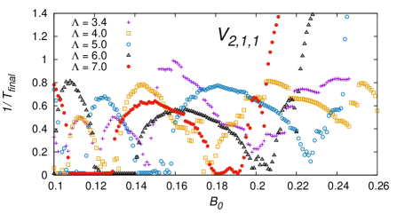
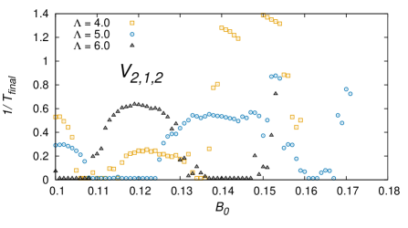
Figure 6: Reciprocal lifetime for links $V_{2,1,1}$ and $V_{2,1,2}$.

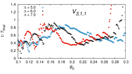
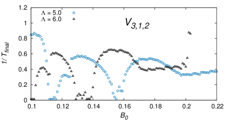
Figure 7: Reciprocal lifetime for links $V_{3,1,1}$ and $V_{3,1,2}$.

III Numerical results

The numerically determined dependences of the (reciprocal) lifetime on parameter $B_{0}$ for fixed values of $\Lambda$ for different knots, unknots, and links are shown in Figs. 1-7. Let us comment on these figures, which are, in fact, the main results of this study.

It should be observed above all that a certain irregularity in the positions of points on the graphs (especially for not very small values of $B_{0}$) can apparently be explained by the noticeable difference between the initial conditions and the steady-state configurations.

It should be emphasized that the calculated reciprocal lifetime is not the instability increment because the initial and final amplitudes of unstable modes have not been fixed; actually, such modes themselves are unknown. The lifetime generally depends on the choice of the initial perturbations of the shape of torus vortices. Only those (most interesting) segments of the graphs, in which the points are close to the horizontal axis, are more or less independent of this choice.

Typical values of $1/T_{\rm final}$ in all cases are on the order of unity. However, some graphs contain small but finite segments on which the reciprocal lifetime does not exceed the small value of $1/T_{\rm max}$. In the vicinity of the edges, the reciprocal lifetime exhibits an approximately root dependence. These are precisely the sought quasi-stability zones. These zones usually appear upon an increase in $\Lambda$, when adjacent parametric resonances of the dynamic system stop overlapping. Such a mechanism of the emergence of quasi-stable zones can be seen most clearly for knot ${\cal T}_{3,2}$, unknot ${\cal U}_{2,1}$, and the simplest link of two rings $V_{2,1,1}$. For many other $V_{n,p,q}$, the quasi-stability windows do not appear at all. In particular, ${\cal T}_{4,q}$, and ${\cal T}_{5,q}$, unknots ${\cal U}_{p\geq 3,1}$, and three rings in configuration $V_{3,1,1}$ are unstable almost in all cases.

The upper panel in Fig. 1 shows that for a fixed value of $\Lambda$, the difference in the results corresponding to different values of $\delta$ is quite small in accordance with the above remark. However, the difference still exists because short-wavelength excitations of the shape of a filament, which undoubtedly “feel” the difference between different values of $\delta$, appear due to nonlinear interactions over long time intervals. For this reason, the maximally accurate simulation based on Eqs. (4) apparently still requires the use of original (non-redefined) parameters $\xi$ and $\Lambda_{0}$. This remark does not contradict the main conclusion concerning the existence of quasi-stable regions on the plane of parameters $(B_{0},\Lambda)$.

It is interesting to note that in some cases, quasi-stable zones are located at large values of $B_{0}=$ 0.16–0.20, for which the initial torus cannot be treated as thin any longer. In this case, the difference between the initial conditions and steady-state solutions turns out to be so large that we can speak on the preservation of the shape of vortices only on the average. In fact, vortex filaments oscillate quite strongly in the nonlinear regime; however, these oscillations astonishingly do not cause the degradation of the system for a long time. For example, in some auxiliary calculations, vortex knots and links with parameters from such stability zones propagated without noticeable changes over distances exceeding thousands of initial radii $R_{0}$. The existence of such solutions appears as the most nontrivial result of this study.

IV Conclusions

Thus, the numerical experiments described above revealed the existence of quite long-lived configurations for some types of torus vortex knots and links. These results undoubtedly extended our knowledge concerning a “venerable” fluid-dynamics problem. In addition, these results are aesthetically attractive. At the same time, a large number of new questions appear because a rigorous theoretical description of this phenomenon does not exist at this stage. It is still unclear whether it would be possible in the nearest future to prepare and observe such quasi-stable quantum vortex structures experimentally.

References

- (1) W. Thomson (Lord Kelvin), Proc. R. Soc. Edin. 9, 59 (1875).
- (2) D. Kleckner and W. T. M. Irvine, Nature Physics 9, 253 (2013).
- (3) R. L. Ricca, D. C. Samuels, and C. F. Barenghi, J. Fluid Mech. 391, 29 (1999).
- (4) F. Maggioni, S. Alamri, C. F. Barenghi, and R. L. Ricca, Phys. Rev. E 82, 026309 (2010).
- (5) O. Velasco Fuentes, Theor. Comput. Fluid Dyn. 24, 189 (2010).
- (6) A. Romero Arteaga, Vórtices eslabonados cuasi-estacionarios, Master’s thesis, CICESE, Ensenada, Mexico (2011).
- (7) O. Velasco Fuentes and A. Romero Arteaga, J. Fluid Mech. 687, 571 (2011).
- (8) D. Proment, M. Onorato, and C. F. Barenghi, Phys. Rev. E 85, 036306 (2012).
- (9) D. Proment, M. Onorato, and C. F. Barenghi, J. Phys.: Conf. Ser. 544, 012022, (2014).
- (10) P. Clark di Leoni, P. D. Mininni, and M. E. Brachet, Phys. Rev. A 94, 043605 (2016).
- (11) D. Kleckner, L. H. Kauffman, and W. T. M. Irvine, Nature Physics 12, 650 (2016).
- (12) V. P. Ruban, JETP Letters 107(5), 307 (2018).
- (13) K. W. Schwarz, Phys. Rev. B 31, 5782 (1985).
- (14) M. Tsubota, T. Araki, and S. K. Nemirovskii, Phys. Rev. B 62, 11751 (2000).
- (15) A. W. Baggaley and C. F. Barenghi, Phys. Rev. B 83, 134509 (2011).