Strongly coupled electron fluids in the Poiseuille regime

Abstract

In the context of describing electrons in solids as a fluid in the hydrodynamic regime, we consider a flow of electrons in a channel of finite width, i.e. a Poiseuille flow. The electrons are accelerated by a constant electric field. We develop the appropriate relativistic hydrodynamic formalism in 2+1 dimensions and show that the fluid has a finite dc conductivity due to boundary-induced momentum relaxation, even in the absence of impurities. We use methods involving the AdS/CFT correspondence to examine the system in the strong-coupling regime. We calculate and study velocity profiles across the channel, from which we obtain the differential resistance $dV/dI$. We find that $dV/dI$ decreases with increasing current $I$ as expected for a Poiseuille flow, also at strong coupling and in the relativistic velocity regime. Moreover, we vary the coupling strength by varying $\eta/s$, the ratio of shear viscosity over entropy density. We find that $dV/dI$ decreases when the coupling is increased. We also find that strongly coupled fluids are more likely to become ultra-relativistic and turbulent. These conclusions are insensitive to the presence of impurities. In particular, we predict that in channels which are clearly in the hydrodynamic regime already at small currents, the DC channel resistance strongly depends on $\eta/s$.

I Introduction

In recent years, hydrodynamic behavior in electron systems has received considerable interest from both theoretical and experimental condensed matter physics. Narozhny et al. (2017); Lucas and Fong (2017). Experimentally, the hydrodynamic regime was first reached in (Al,Ga)As high mobility wires more than two decades ago when the Gurzhi effect was observed Molenkamp and de Jong (1994a, b); de Jong and Molenkamp (1995), and more recently in several other materials including graphene Crossno et al. (2015); Moll et al. (2016); Bandurin et al. (2016); Nam et al. (2017). The Gurzhi effect Gurzhi (1968) in such wires is a crossover between boundary-dominated scattering (the Knudsen regime) at low densities and hydrodynamic behavior at higher densities (the Poiseuille regime). It manifests itself as a crossover in the channel resistance as a function of the applied current: The channel resistance rises in the Knudsen regime, while it falls in the Poiseuille regime. In spite of the experimental successes mentioned, observing clear signs of viscous hydrodynamic transport or exactly measuring the value of the viscosity turns out to be challenging in electronic systems in general . One key reason is that the interpretation of averaged observables such as e.g. voltages in nonlocal measurements (proposed e.g. as a signature of hydrodynamic whirlpools Levitov and Falkovich (2016)) depend crucially on the boundary conditions Pellegrino et al. (2016) of the measurement setup. Nevertheless, theoretical proposals exist to measure the viscosity using non-local transport in Hall bars Torre et al. (2015), rheometers Tomadin et al. (2014), and AC transport Moessner et al. (2018). Also, in the presence of impurity scattering, the interesting hydrodynamic regime may actually be restricted to a narrow range of parameters, as can e.g. be seen from the weak coupling phase diagram of the relativistic Gurzhi effect derived from kinetic theoryKashuba et al. (2018).

In order to make progress towards resolving some of the issues mentioned, in the present paper we investigate hydrodynamic behavior as realized by a Poiseuille flow in a relativistic strongly coupled system. This is conveniently done by using methods of the AdS/CFT correspondence Maldacena (1998); Gubser et al. (1998); Witten (1998). In particular, we present a model where we are able to investigate the dependence of the flow on the coupling strength starting from very large couplings by varying only one parameter, which is the ratio of shear viscosity over entropy density.

The AdS/CFT conjecture provides universal predictions for observables of strongly coupled and correlated systems Casalderrey-Solana et al. (2014); Ammon and Erdmenger (2015); Zaanen et al. (2015); Hartnoll et al. (2016). One such prediction is that the low-energy excitations of strongly coupled gapless systems described via AdS/CFT are governed by the laws of hydrodynamics. The hydrodynamic equations of motion are conservation laws for the only long-lived excitations expected in a strongly interacting system. These are the long-wavelength, low-energy excitations of conserved quantities such as e.g. energy, momentum, or charge. This is not surprising since a very strongly coupled gapless system at low energies is expected to have a very short equilibration time and mean free path beyond which the system behaves hydrodynamically. In the absence of additional conserved quantities or other parametric suppressions by ratios of scales, the equilibration time will be of order Zaanen (2004)

$$\tau_{eq}\sim\frac{\hbar}{k_{B}T}\,.$$ (I.1)

In particular, (I.1) holds in all rotationally invariant holographic models of electronic transport with a stable ground state. In these models, the approach to local equilibrium is governed by the most long-lived non-hydrodynamical quasinormal mode of the dual black brane, which has a lifetime of order (I.1). However, an equilibration time of order (I.1) is not a necessary condition for hydrodynamic behaviour. The conditions of applicability of hydrodynamics as a low-energy effective theory will be discussed in sec. II.1.

The AdS/CFT correspondence allows not only to derive hydrodynamics from perturbations of black branes in AdS space-time Bhattacharyya et al. (2008a, b, 2009); Blake (2015), but also the values of the transport coefficients (viscosities, conductivities, etc.). Calculating the shear viscosity from AdS/CFT for rotationally invariant systems Policastro et al. (2001), the ratio of shear viscosity to entropy density takes a universal value

$$\frac{\eta}{s}=\frac{1}{4\pi}\frac{\hbar}{k_{B}}\,,$$ (I.2)

independent of the other parameters of the system such as e.g. temperature or chemical potential. It is conjectured thatKovtun et al. (2005) (I.2) constitutes a universal minimal bound for all interacting quantum systems,

$$\frac{\eta}{s}\geq\frac{1}{4\pi}\frac{\hbar}{k_{B}}\,.$$ (I.3)

This so-called Kovtun-Son-Starinets (KSS) bound can be motivated by e.g. scaling arguments in quantum critical phases Zaanen (2004); Delacrétaz et al. (2018); Hartman et al. (2017), and ultimately should be related to fundamental properties of transport in interacting quantum systems.

It is of great interest to experimentally test the predictions (I.1)-(I.3). In heavy-ion collision experiments, $\eta/s$ was experimentally found to be of the same order as (I.2) Song et al. (2011), albeit with large error bars. The main issue in extracting $\eta/s$ in heavy-ion collisions is the very indirect dependence of the final state particle distributions measured in the detector on the value of the hydrodynamic transport coefficients. The transport properties of strongly coupled and correlated electron systems in the hydrodynamic regime could hence provide a more direct window into the strong coupling regime of interacting quantum systems. In particular, two-dimensional Dirac materials such as graphene Novoselov et al. (2005) or the surface states of topological insulators such as e.g. HgTe König et al. (2007), as well as Weyl- and Dirac semimetals in three spatial dimensions Klinkhamer and Volovik (2005); Volovik (2006); Wan et al. (2011) are of interest here due to their relativistic band structures. If electron-electron interactions are the fastest way for electrons to redistribute their energy and momentum and equilibrate, the electrons should form a relativistic fluid governed by the equations of relativistic hydrodynamics.

The ratio $\eta/s$ depends explicitly on the coupling constant, and hence serves as a measure of the interaction strength itself. In the weak coupling regime, $\eta/s$ can be calculated in perturbation theory. Increasing the interactions, one expects the system to enter the strongly coupled regime and saturate the bound (I.3). Kinetic theory calculations of $\eta/s$ for Coulomb interacting two-dimensional Dirac materials support this picture: At charge neutrality and to first order in the effective temperature dependent Coulomb coupling $\alpha(T)$, $\eta/s$ was found to beFritz et al. (2008); Müller et al. (2009)

$$\frac{\eta}{s}=\frac{C_{\eta}\pi}{9\zeta(3)}\frac{1}{\alpha^{2}(T)}\frac{\hbar}{k_{B}}\approx\frac{1.64}{4\pi}\frac{1}{\alpha^{2}(T)}\frac{\hbar}{k_{B}}\,,$$ (I.4)

where $C_{\eta}\approx 0.449$ is a numerical constant. As $\alpha$ enters the strong coupling regime, $\alpha\simeq 1$, $\eta/s$ is expected to approach the holographic value (I.2). The behavior of $\eta/s$ as a function of $\alpha$ is shown in fig. 2. Hence, if the hydrodynamic regime can be reached experimentally in materials with large Coulomb coupling, and if observables sensitive to $\eta/s$ can be found, it will become possible to experimentally test the AdS/CFT prediction (I.2) in hydrodynamic electron systems.

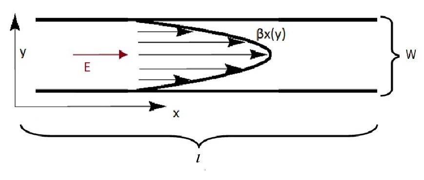
Figure 1: Schematic flow of charged particles along a $xy$ plane in the Poiseuille flow. The fluid in this regime is incompressible and has zero velocity at the boundaries, such that the maximum speed is attained in the middle of the channel. In the $\beta_{x}\ll v_{F}$ approximation, the profile acquires a characteristic parabolic shape.

In view of further progress in detecting hydrodynamic behaviour, the channel setup Molenkamp and de Jong (1994a, b); de Jong and Molenkamp (1995); Kashuba et al. (2018) showing the two-dimensional Gurzhi effect Gurzhi (1968) described above is probably the simplest setup possible. In hydrodynamical terms, this corresponds to the simplest flow geometry in which a controlled hydrodynamic flow can be achieved, such that it may be easiest to find observables sensitive to changes of the value of the ratio $\eta/s$ alone. The channel setup consists of two parallel boundaries with prescribed boundary conditions, and a laminar flow in between in the presence of an electric field along the channel direction. Two different choices of boundary conditions are common:Lucas and Fong (2017) The boundary condition of vanishing velocity at the channel wall gives rise to the Poiseuille flow, which is depicted in Fig. 1. The choice of vanishing stress at the boundaries leads to an Ohmic flow.

In our work, we take the channel setup as a starting point and provide a detailed study of parametric effects for a relativistic charged Poiseuille flow in the absence of parity or time reversal breaking. We in particular study the dependence on the value of $\eta/s$ of the Poiseuille flow and observables derived from it such as the differential wire resistance. We vary $\eta/s$ independently of the impurity relaxation time, channel width, chemical potential, temperature and external electrical field. Varying the value of $\eta/s$ from (I.2) to larger values allows us in particular to interpolate from the strong to the intermediate coupling regime, and in this way to search for physical signatures of strongly coupled fluids.

In the original form of the AdS/CFT correspondence, the strong coupling regime associated with (I.2) involves taking the limit in which the coupling strength is infinite. Moving to lower coupling strengths through changing the value of $\eta/s$ requires us to specify the coupling dependence of this ratio. We make the assumption that $\eta/s$ is a monotonically decreasing function of the coupling constant $\alpha$, i.e. we interpolate from the extremely strongly coupled regime towards intermediate weaker coupling strengths. Our guiding principle for this interpolation is the known behavior at weak and very strong coupling, as shown in Fig. 2. We further assume that hydrodynamics is applicable throughout this interpolation. Further support for the interpolation is given by the following argument based on the perturbative result (I.4): In the strong coupling regime, higher orders in $\alpha$ will become as important as the lowest order term in (I.4). Nevertheless, since $\eta/s$ has the interpretation of the rate of diffusive momentum transfer between adjacent fluid layers normalized to the effective numbers of degrees of freedom, we expect higher orders only to enhance momentum transfer and hence decrease $\eta/s$. Our analysis does not depend on the exact form of the interpolating function $\eta/s(\alpha)$, only on its monotonicity.

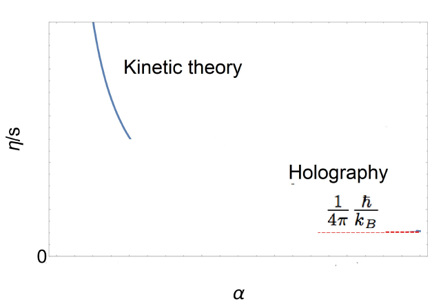
Figure 2: Sketch of $\eta/s$ as a function of the coupling strength. At low $\alpha$, perturbation theory predicts a $1/\alpha^{2}$ behavior, which asymptotes to a constant value in the large $\alpha$ limit. Holography predicts the value of this constant to be $\hbar/4\pi k_{B}$ .

We find that the channel resistance depends on the ratio $\eta/s$ rather than on $\eta$ alone: Solving the fully relativistic equations, which do not admit a simple analytic solution as in the non-relativistic limit,Lucas and Fong (2017) we confirm that the differential resistance indeed does decrease with decreasing $\eta/s$ for all velocity regimes. Moreover, $\eta/s$ is a good measure for the momentum transfer between fluid layers normalized to the central charge and temperature, i.e. to the number of effective degrees of freedoms in the momentum transfer. We find that the resistance increases when reducing the coupling. We confirm this by changing $\eta/s$ away from its infinite strong coupling value $\hbar/(4\pi k_{B})$.

The main focus of our work is the analysis of the fully relativistic Poiseuille flow. In addition we also studied the effect of momentum relaxation, this however only in the non-relativistic regime. In both cases, we calculate the velocity profile, the differential resistance of the channel and the wall relaxation time defined below.

In the absence of momentum-relaxing impurities, we find that $\eta/s$ has a strong effect on the fluid flows in both the non-relativistic and relativistic velocity regimes. In particular strongly coupled holographic fluids satisfying (I.2) flow faster compared to their weakly coupled counterparts. The reason is that in the absence of impurities, the only way for the fluid to lose momentum is through the boundaries, which absorb the momentum density. The rate of momentum transfer between adjacent fluid layers is controlled by $\eta/s$, and hence the momentum transfer to the boundaries becomes as inefficient as it can be for fluids satisfying (I.2). The rate of momentum loss through the boundaries is characterized by an associated wall relaxation time scale $\tau_{w}$. We calculate the wall relaxation time scale and find that it is longer for strongly coupled holographic fluids than for weakly coupled ones. We furthermore calculate the differential channel resistance $dV/dI$, and find as expected that it decreases with decreasing $\eta/s$. Holographic fluids restricted to channels hence show lower channel resistance than weakly coupled ones.

We also consider the effect of momentum relaxing impurities on the Poiseuille flow. In microscopic descriptions of real-world condensed matter systems, the physics of impurities in general depends on the nature of the scattering potential (extended, hard, soft, long or short range etc.). A similar model dependence is also inherent in holographic models, which depend on the precise mechanism used to break translation invariance and hence momentum conservation. Nevertheless, in both cases the relaxation time approximation, i.e. the assumption of a constant relaxation time, often proves to be a good and universal approximation to the weak impurity limit. In our setup, we dial the impurity relaxation time independently of the other parameters of the system, in order to distinguish impurity effects from hydrodynamic ones. Hydrodynamics is only a good description if the impurity relaxation scale is a slow scale in the system, slower than the equilibration time (I.1) and the time-scale of hydrodynamic fluctuations. The latter is given by the gradients of hydrodynamic fields velocity, temperature, and chemical potential. If the momentum relaxation time scale is short compared to the momentum transport time set by $\eta/s$, we find a crossover to an impurity-dominated Ohmic regime even for the zero velocity boundary conditions characterizing the Poiseuille flow. The crossover happens if the ratio

$$\Pi=\frac{1}{T\tau_{\rm imp}}\frac{\eta}{s}$$ (I.5)

is of ${\cal O}(1)$. The Poiseuille regime occurs for $\Pi\ll 1$. In the Ohmic regime $\Pi\gg 1$, hydrodynamics is no longer valid as a low-energy effective theory.

To conclude the introduction, we summarize the new results of our work:

• We performed a numerical as well as analytical analysis of relativistic hydrodynamics for a fluid confined in a two-dimensional wire geometry, in addition to considerations for the non-relativistic case. We find Poiseuille behavior for all velocities, and in particular also in the relativistic regime. The importance of considering the relativistic regime can be seen from the fact that the differential resistance drops to zero in the ultrarelativistic limit, in which the fluid velocity approaches the Fermi velocity $|\vec{v}|\rightarrow v_{F}$, purely as a consequence of the kinematics of special relativity.

• We find that the channel resistance strongly scales with the ratio of shear viscosity over entropy density $\eta/s$, which is the properly normalized measure of momentum transfer between fluid layers per effective degree of freedom. Holographic strongly coupled fluids, for which $\eta/s\simeq 1/4\pi$, exhibit smaller differential resistance than conventional weakly coupled fluids. The channel resistance scales with $\eta/s$ also in the fully relativistic regime.

• We calculate the time scale associated to momentum relaxation through the walls, i.e. the time scale associated with the rate of momentum loss through the channel walls for zero velocity boundary conditions, both in the nonrelativistic and relativistic regimes. The wall relaxation time is inversely proportional to $\eta/s$, even in the relativistic regime. In the non-relativistic regime, this behavior may be seen analytically

• We examine the onset of turbulence in the channel by calculating the Reynolds number of our flows. We find that for the input parameters typical in current experimental realizations, the flow is laminar. The Reynolds number may also be significantly increased by increasing the channel width by an order of magnitude. Transitioning to a pre-turbulent regime is, however, not ruled out for setups with channel constrictions or obstacles placed in the flow. Moreover, we find that impurities affect the onset of turbulence by bounding the values the Reynolds number can reach. We present explicit formulae for these bounds.

In addition, our analysis is phenomenological in nature and relies on the applicability of hydrodynamics alone. It is not restricted to any particular Dirac metal such as graphene, but also applies, for example, to strange metals and other strongly correlated materials. In particular the strange metallic phases in high temperature superconductors are expected to behave hydrodynamically,Davison et al. (2014) and our analysis is hence applicable.

This paper is organized as follows: In sec. II we review the equations of relativistic hydrodynamics (sec. II.1), as well as the pieces of the AdS/CFT correspondence necessary to understand our analysis (sec. II.2). In sec. III, we then discuss the effect of the finite channel width leading to the the Poiseuille flow (sec. III.1), the effect of momentum relaxation through the walls (sec. III.2). Sec. IV is devoted to the analysis of the flow velocity profiles and the differential channel resistance in the absence of impurities. Sec. V then includes momentum relaxing impurities into the analysis. In section VI, we present preliminary results on the onset of turbulence in Gurzhi-type channel setups. Finally, in sec. VII we discuss our results and give an outlook to possible future research. We estimate in appendix  B the Reynolds number both in the nonrelativistic and ultrarelativistic limits.

II Relativistic hydrodynamics and the AdS/CFT correspondence

II.1 Relativistic hydrodynamics

In this section we review elements of hydrodynamics relevant to our analysis. Landau and Lifshitz (1987); Romatschke (2010); Luciano Rezzolla (2013) Relativistic hydrodynamics is the effective field theory of long-wavelength low-energy fluctuations of matter in local thermal equilibrium. Its dynamical equations are the conservation laws of energy, momentum and charge. We neglect the imbalance current in relativistic systems, which is approximately conserved at weak coupling and close to charge neutrality. This additional conserved current does not couple to the external electromagnetic field, and hence does not contribute to electric transport. It will however contribute to thermal and thermoelectric transport.Lucas and Fong (2017)

Consider a two-dimensional electron system in a wire geometry of width $W$ and length $l\gg W$. Local thermalization is dictated by the average time between electron-electron collisions $\tau_{\rm ee}$. It is possible to describe the electron gas by means of hydrodynamics if the electron-electron scattering time is the shortest timescale present, and if all other external time-scales are much longer than the time-scale of hydrodynamic fluctuations. Within our setup, we have two additional relevant timescales: the time between electron-impurity collisions, i.e. the momentum relaxation time-scale $\tau_{\rm imp}$, and $W/v_{F}$. The corresponding length scales are obtained by multiplying with the (constant) Fermi velocity $v_{F}$. Therefore, the two-dimensional electron gas will behave as a fluid if, in natural units,

$$\ell_{\rm ee}\ll||\partial_{\nu}(T,\mu,u^{\mu})||\ll\ell_{\rm imp},\,W\,.$$ (II.1)

This is the regime we consider in this work (see again the caveat of footnote 48) .

If the electrons have a relativistic dispersion, the local thermal equilibrium will be described on scales exceeding $\ell_{\rm ee}=v_{F}\tau_{\rm ee}$ by a local temperature $T(x^{\mu})$, a local chemical potential $\mu(x^{\mu})$, and a local relativistic velocity $u^{\mu}(x^{\nu})$, where e.g. $x^{\mu}=(t,x,y)$ for a planar 2+1-dimensional system. The velocity field must be time-like and normalized to the speed of light relevant for the relativistic fluid, which e.g. in case of graphene is the Fermi velocity $v_{F}$ appearing in the dispersion relation of the Dirac particles. We focus on 2+1-dimensional hydrodynamics, as it is relevant to two-dimensional electron systems. In terms of the velocities $(\beta_{x}(x^{\mu}),\beta_{y}(x^{\mu}))$,

$$u^{\mu} =\gamma\left(v_{F},\beta_{x},\beta_{y}\right),\qquad\gamma=\frac{1}{\sqrt{1-\frac{\beta_{x}^{2}+\beta_{y}^{2}}{v_{F}^{2}}}}\,,$$ (II.2)

$$u^{\mu}u_{\mu} =u^{\mu}u^{\nu}\eta_{\mu\nu}=-v_{F}^{2}\,,\quad\eta_{\mu\nu}=\operatorname{diag}(-1,1,1)\,.$$ (II.3)

The equations of relativistic hydrodynamics are the conservation equations for the Lorentz covariant energy-momentum tensor $T_{\mu\nu}$ and the relativistic charge current $j^{\mu}$. In absence of impurities, the covariant energy-momentum and current conservation equations for a fluid in the presence of an external electromagnetic field are

$$\partial_{\mu}T^{\mu\nu} = \frac{h}{e^{3}c}\,j_{\alpha}D^{\nu\alpha}\,,$$ (II.4)

$$\partial_{\mu}j^{\mu} = 0\,.$$ (II.5)

We assume the background metric to be the metric of flat Minkowski space-time, $g_{\mu\nu}=\eta_{\mu\nu}$. $D^{\mu\nu}$ is the electromagnetic displacement tensor, which in 2+1 dimensions takes the form

$$D^{\mu\nu}=e\left(\begin{array}[]{c c c}0&E_{x}\epsilon_{0}\epsilon_{r}c&E_{y}\epsilon_{0}\epsilon_{r}c\\ -E_{x}\epsilon_{0}\epsilon_{r}c&0&-B/\mu_{0}\mu_{r}\\ E_{y}\epsilon_{0}\epsilon_{r}c&B/\mu_{0}\mu_{r}&0\\ \end{array}\right),$$ (II.6)

with $D_{\nu\mu}=\eta_{\nu\alpha}\eta_{\mu\delta}D^{\alpha\delta}$. The electric field, given by $E^{\mu}=h/\left(e^{3}c\right)u_{\alpha}D^{\mu\alpha}$, fulfills $u_{\alpha}E^{\alpha}=0$. The charge density to which the electric field couples is then $v_{F}^{2}e\rho=-j^{\alpha}u_{\alpha}$. Note that while the speed of light relevant for the Lorentz symmetry of the fluid is $v_{F}$, the speed of light relevant for the coupling to the external electromagnetic field is the usual one, $c$. $\epsilon_{0}$, $\mu_{0}$, $\epsilon_{r}$, and $\mu_{r}$ are the dielectric constant of the vacuum, the vacuum permeability, the relative permittivity and the relative permeability in medium.

In order for (II.4)-(II.5) to form a set of equations for the hydrodynamic variables $(T,\mu,u^{\mu})$, we need to specify the stress-energy tensor $T_{\mu\nu}$ and the charge current $j^{\mu}$ in terms of these variables. This is formulated as a derivative expansion around global equilibrium, characterized by constant $T$ and $\mu$, and vanishing velocity in the rest frame, $u^{\mu}=(v_{F},0,0)$. We decompose the stress-energy tensor and charge current in terms of tensor structures parallel and perpendicular to the flow field $u^{\mu}(x)$,

$$T_{\mu\nu}={\cal E}u_{\mu}u_{\nu}+{\cal P}\Delta_{\mu\nu}+(q_{\mu}u_{\nu}{+}q_{\nu}u_{\mu})+t_{\mu\nu},$$ (II.7a)

$$j_{\mu}={\cal N}u_{\mu}+\nu_{\mu}\,,$$ (II.7b)

where $\Delta^{\mu\nu}=u^{\mu}u^{\nu}/v_{F}^{2}+\eta^{\mu\nu}$ is the projector onto the space orthogonal to the flow field. ${\cal E}$, ${\cal P}$, and ${\cal N}$ are Lorentz scalars, $q_{\mu}$, $t_{\mu\nu}$, and $j_{\mu}$ are transverse, $u_{\mu}q^{\mu}=0$, $u_{\mu}t^{\mu\nu}=0$, $u_{\mu}\nu^{\mu}=0$, and $t^{\mu\nu}$ is symmetric and traceless. As for any effective field theory, redefinitions of the fields $(T,\mu,u^{\mu})$ can mix the different terms in (II.7). It is hence important to specify conditions that fix the freedom to redefine the hydrodynamical fields, i.e. to chose a hydrodynamical frame. The most common frame is the Landau frame. In Landau frame, the local energy density in equilibrium $\epsilon$ is identified with ${\cal E}$ via the condition $T^{\mu\nu}u_{\mu}=-\varepsilon u^{\nu}$, and the density of conserved charge $e\rho$ is identified with ${\cal N}$ via $j^{\alpha}u_{\alpha}=-v_{F}^{2}e\rho$. The fluid is comoving to the energy flow, amounting to $q^{\mu}=0$ in (II.7a). We exclusively work in Landau frame in this paper.

Having fixed the frame, the expansion up to first order in derivatives of $u^{\mu}$ for $T^{\mu\nu}$ and $j^{\mu}$ for a rotationally invariant charged fluid in $2+1$ dimensions is

$$T^{\mu\nu} =T^{\mu\nu}_{\rm(ideal)}+T^{\mu\nu}_{\rm(viscous)},$$ (II.8)

$$T^{\mu\nu}_{\rm(ideal)} =\varepsilon\,u^{\mu}u^{\nu}/v_{F}^{2}+p\Delta^{\mu\nu}\,,$$ (II.9)

$$T^{\mu\nu}_{\rm(viscous)} =-\eta\Delta^{\mu\alpha}\Delta^{\nu\beta}\left(2\partial_{(\alpha}u_{\beta)}-\Delta^{\alpha\beta}\partial_{\sigma}u^{\sigma}\right)$$

$$\quad-\xi\Delta^{\mu\nu}\partial_{\gamma}u^{\gamma},$$ (II.10)

$$j^{\mu} =e\rho u^{\mu}+\sigma_{Q}\left(E^{\mu}-T\Delta_{\mu\nu}\partial^{\nu}\frac{(\mu/e)}{T}\right)\,,$$ (II.11)

where $\varepsilon,p,\rho$ are energy density, pressure and number density of the fluid in local equilibrium. $\sigma_{Q}$ is the intrinsic quantum critical conductivity due to the counterflow of electrons and holes Fritz et al. (2008). $\eta$ and $\xi$ are the shear and bulk viscosities. For application to Dirac materials such as e.g. graphene, which are approximately scale invariant, we neglect the bulk viscosity, $\xi=0$.

In the presence of momentum relaxing impurities, the classical Drude model alters the right hand side of the Newton equation $F=m\dot{v}$ by adding a friction term,

$$m\dot{v}\to m\dot{v}+\frac{m}{\tau_{\rm imp}}v.$$ (II.12)

We first project (II.4) into the direction of time given by the velocity field $u^{\mu}$ and perpendicular to it by multiplying with $u^{\mu}$ and $\Delta^{\mu\nu}$, respectively,

$$u_{\nu}\partial_{\mu}T^{\mu\nu} = \frac{h}{e^{3}c}u_{\nu}j_{\alpha}D^{\nu\alpha},$$ (II.13)

$$\Delta_{\rho\nu}\partial_{\mu}T^{\mu\nu} = \frac{h}{e^{3}c}\Delta_{\rho\nu}j_{\alpha}D^{\nu\alpha}.$$ (II.14)

The first equation enforces the conservation of energy, whereas the second equation is the relativistic version of the Navier-Stokes equation. We add a loss term to the right-hand side of the Navier-Stokes equations (II.14),

$$u_{\nu}\partial_{\mu}T^{\mu\nu} = \frac{h}{e^{3}c}u_{\nu}j_{\alpha}D^{\nu\alpha},$$ (II.15)

$$\Delta_{\rho\nu}\partial_{\mu}T^{\mu\nu} = \frac{h}{e^{3}c}\Delta_{\rho\nu}j_{\alpha}D^{\nu\alpha}-\Delta_{\rho\nu}\frac{T^{t\nu}}{v_{F}\tau_{\rm imp}}.$$ (II.16)

The momentum relaxation time $\tau_{\rm imp}$ can be thought of arising from electron-impurity scattering in the relaxation time approximation. We henceforth assume that this is the only relaxation time entering the relativistic hydrodynamic equations. We in particular assume that energy relaxation is sufficiently fast such that in the non-equilibrium steady states considered, the non-equilibrium energy density is close to the energy density in local thermal equilibrium at the electron temperature. This is supported by quantum criticality arguments Zaanen (2004), as well as measurements of scattering times in materials with strong correlations Bruin et al. (2013); Gooth et al. (2017).

II.2 Strongly coupled fluids in AdS/CFT

In order to solve the hydrodynamic equations (II.15) and (II.16), we need to specify the thermodynamic variables that enter the constitutive relations (II.9), (II.1), (II.11). For strongly coupled fluids, it is natural to take these values from the AdS/CFT correspondence. In appendix A we detail how AdS/CFT determines them for a strongly coupled field theory at finite temperature and density.

In this approach, the thermodynamic variables read

$$\varepsilon = \frac{L^{2}}{8\pi G_{4}}\hbar\,v_{F}\frac{r_{H}^{3}}{L^{6}},\quad p=\frac{L^{2}}{16\pi G_{4}}\hbar\,v_{F}\frac{r_{H}^{3}}{L^{6}},$$ (II.17)

$$\rho = \frac{L^{2}}{64\pi G_{4}}\left(\frac{r_{H}}{L^{2}}\right)\frac{\mu}{\hbar v_{F}},\quad s=\frac{k_{B}}{4G_{4}}\frac{r_{H}^{2}}{L^{2}},$$ (II.18)

where $L$ is the $AdS_{4}$ radius and $G_{4}$ is the Newton constant, as explained in detail in appendix A. In particular,

$$\frac{r_{H}}{L^{2}}=\frac{1}{6}\frac{k_{B}T}{\hbar\,v_{F}}\left(4\pi+\sqrt{16\pi^{2}+\frac{3\mu^{2}}{k_{B}^{2}T^{2}}}\right),$$ (II.19)

with $r_{H}$ the radius of the black hole horizon.

The quantities given by (II.17) and (II.18) satisfy the Gibbs-Duhem relation

$$\varepsilon+p=\mu\rho+Ts.$$ (II.20)

In the AdS/CFT approach, the charged fluid is strongly coupled, such that $\eta/s$ is small. We take a phenomenological approach of varying the coupling towards weaker and intermediate values as follows: Starting from the holographic value of $\eta/s=\hbar/4\pi k_{B}$, we then slowly increase $\eta/s$ to investigate the behavior of the fluid when moving from the holographic strongly coupled regime towards weaker intermediate coupling. In the calculation of physical variables presented below, we fix the overall coefficients of physical observables using the AdS/CFT approach given in appendix A.

III Finite size effects

III.1 Poiseuille flow

We now investigate the physical effects that arise from the motion of a fluid in a channel of finite size. Consider an incompressible fluid moving along a wire of width $W$ and length $l$. We may think of the fluid as a superposition of fluid layers along the width of the channel. The fluid’s flow is laminar if these layers never mix. A particular kind of laminar flow is the Poiseuille flow characterized by the no-slip boundary conditions,

$$u^{i}(y)\Big{|}_{y=W}=0,\quad u^{i}(y)\Big{|}_{y=0}=0.$$ (III.1)

Simply stated, the velocity vanishes at the boundaries. A parametrization of the velocity $u^{\mu}$ is given by

$$u^{\mu}=\gamma(y)\left(v_{F},\beta_{x}(y),0\right),\qquad\gamma=\frac{1}{\sqrt{1-\frac{\beta_{x}(y)^{2}}{v_{F}^{2}}}}.$$ (III.2)

This Ansatz is incompressible,

$$\partial_{\sigma}u^{\sigma}=\partial_{0}u^{0}+\partial_{i}u^{i}=\frac{1}{v_{F}}\partial_{t}u^{t}+\partial_{i}u^{i}=0.$$ (III.3)

Moreover, the boundary condition (III.1) is equivalent to

$$\beta_{x}(y)\Big{|}_{y=W}=0,\quad\beta_{x}(y)\Big{|}_{y=0}=0.$$ (III.4)

Now we derive the hydrodynamic equations in terms of $\beta_{x}$ from (II.16). Focusing on the case of a homogeneous external electric field pointing along the $x$-direction, the current density (II.11) reads

$$j^{\mu}=ev_{F}\gamma\left(\rho+\frac{h\epsilon_{0}}{e^{3}}\frac{\beta_{x}}{v_{F}}\epsilon_{r}\sigma_{Q}E^{x},\rho\frac{\beta_{x}}{v_{F}}+\frac{h\epsilon_{0}}{e^{3}}\epsilon_{r}\sigma_{Q}E^{x},0\right).$$ (III.5)

Here $\epsilon_{0}\epsilon_{r}$ is the electric permittivity of the fluid, $\rho$ its number density, $v_{F}$ its Fermi velocity, and $\sigma_{Q}$ its quantum critical conductivity. Decomposing (II.16) into components, we obtain two independent equations

$$0 =\frac{\eta}{s}\left[\beta_{x}^{\prime\prime}+\frac{2}{v_{F}^{2}}\gamma^{2}\beta_{x}\beta_{x}^{\prime 2}\right]+\frac{1}{\gamma}\left(v_{F}\epsilon_{r}\frac{\epsilon_{0}\,h}{e}\frac{E_{x}}{\gamma}\frac{\rho}{s}-\frac{p+\varepsilon}{s\tau_{\rm imp}}\frac{\beta_{x}}{v_{F}^{2}}\right),$$ (III.6)

$$0 =p^{\prime}-\frac{\eta}{\tau_{\rm im}v_{F}^{2}}\gamma^{3}\beta_{x}\beta_{x}^{\prime}.$$ (III.7)

We find a dynamical equation for the velocity profile (III.2), as well as a relativistic form of the Hagen-Poiseuille equation for the pressure. For strongly coupled theories, the ratio $\eta/s$ is fixed to a constant value, which is why we divided (III.6) by the entropy density $s$. The solution to the pressure equation (III.7) is given by

$$p(y)=p_{0}+C+\frac{\eta}{\tau_{\rm imp}}\gamma(y).$$ (III.8)

Here $C$ is an integration constant of (III.8) which will be fixed shortly. Note that the ratio ${\eta}/{\tau_{\rm imp}}$ controlling the pressure shift will be small in the parameter regime of applicability of hydrodynamics (II.1). The non-equilibrium fluid pressure (III.8) will hence be close to the thermodynamic one as e.g. derived from the AdS solution (II.18), $p\approx p_{0}(\mu,T)$. Therefore, we may use the homogeneous thermodynamic variables (II.18) even in the presence of impurities, as long as we restrict ourselves to small electric fields and non-relativistic flows. In that limit, the pressure shift becomes constant in the direction $y$ perpendicular to the channel,

$$p=p_{0}+C+\frac{\eta}{\tau_{\rm imp}},$$ (III.9)

since $\gamma\sim 1$. A similar constant pressure shift due to impurities has also been observed in holographic models of momentum relaxationVegh (2013); Andrade and Withers (2014). We emphasize that in our work as well as in the cited paper, the equation of state of the fluid is given by the Gibbs-Duhem equation.

The pressure as defined in (III.8) must smoothly reduce to the equilibrium pressure in absence of flow as the velocity profile tends to zero, $\beta_{x}(y)=0$. We therefore adjust the integration constant in (III.8), and identify the resulting pressure $p$ in the $\beta_{x}(y)=0$ limit as the thermodynamical pressure that enters into the Gibbs-Duhem relation II.20. The thermodynamic pressure $p$ in presence of a flow gradient is thus

$$p=p_{0}+\frac{\eta}{\tau_{\rm imp}}\left[\gamma(y)-1\right].$$ (III.10)

We note that the pressure shift in (III.8) can become large with respect to $p_{0}$ and strongly $y$-dependent. This can lead to observable consequences such as a voltage drop between the middle of the channel and the channel walls. Notice that the pressure shift (III.10), is a genuine relativistic effect.

III.2 Momentum relaxation through the walls

In this subsection we will discuss how the Gurzhi channel setup of Fig. 1 allows for momentum relaxation through the boundaries. We will in particular introduce and calculate the relaxation time scale $\tau_{w}$ associated to the outflow of momentum through the channel walls. To the best of our knowledge, such an explicit computation has not been performed in the literature before.

For a stationary flow, if we suddenly turn off the electric field, momentum will diffuse through the walls located at $y=0$ and $y=W$. Therefore, the $x$ component of the fluid momentum along the velocity direction changes due to momentum loss through the boundaries and through collisions with impurities, i.e.

$$\frac{1}{v_{F}}\partial_{t}T^{tx}=\partial_{y}T^{yx}-\frac{T^{tx}}{v_{F}\tau_{\rm imp}}\,.$$ (III.11)

We parametrize the rate of momentum loss through the boundaries by $\tau_{w}$. Analogously to $\tau_{\rm imp}$, the impurity scattering rate $\tau_{w}$ is also related to momentum loss. However, this particular form of momentum diffusion appears only from finite size effects, unlike $\tau_{\rm imp}$ which can also be present in bulk samples.

If we approximate the time derivative that appears in (III.11) by

$$\partial_{t}T^{tx}\simeq\frac{T^{tx}}{\tau_{w}},$$ (III.12)

and integrate along the $y$ direction, we obtain

$$\frac{1}{v_{F}}\int^{W}_{0}dy\,T^{tx}\left(\frac{1}{\tau_{w}}+\frac{1}{\tau_{\rm imp}}\right)=T^{xy}\Big{|}_{0}^{W}.$$ (III.13)

From the no-slip conditions (III.4), we have that

$$T^{xy}\Big{|}_{0}^{W}=-\eta\beta^{\prime}_{x}(y)\Big{|}_{0}^{W}.$$ (III.14)

The channel geometry with no-slip boundary conditions allows for momentum relaxation through the walls, via the boundary term on the right hand side of (III.13) and (III.14). Due to the no-slip boundary conditions, $\beta_{x}^{\prime}(y)>0$ and hence momentum is not conserved any more. Therefore, the channel walls act as a sink of momentum for the fluid. Substituting $T^{tx}$ from (II.9) into (III.13), we obtain

$$\int_{0}^{W}dy\,\,\frac{\beta_{x}}{v_{F}}\left(p+\varepsilon\right)\gamma^{2}\left(\frac{1}{\tau_{w}}+\frac{1}{\tau_{\rm imp}}\right)=-\eta\beta^{\prime}_{x}(y)\Big{|}_{0}^{W}.$$ (III.15)

Equation (III.15) can be solved for $\tau_{w}$ once the velocity profile and thermodynamic variables are specified. Mechanisms that lead to momentum dissipation have been widely discussed in the literatureAndrade and Withers (2014); Davison (2013). However, we stress that the momentum relaxation effects discussed there are not related to wall momentum relaxation, which is different in nature. This can be seen from our hydrodynamic simulations, which lead to a finite and well-defined channel resistance even in the absence of momentum relaxing impurities. This is to be contrasted with the case of the infinitely extended system, where finite charge density without local momentum relaxation leads to an infinite DC conductivity, i.e. vanishing DC resistivity.

IV Flow and differential resistance in the absence of impurities

IV.1 Velocity profiles

We now proceed to the calculation of the velocity profile $\beta_{x}$ of the fluid as a function of the coordinate $y$ perpendicular to the fluid motion. To do this, we numerically integrate the Navier-Stokes equation (III.6) with the boundary conditions (III.4). This will allow us to determine how the fluid profile depends on the applied electric field, the temperature, the chemical potential and the width of the wire. Moreover, from the velocity profile we will calculate the differential resistance $dV/dI$. In this section, we will consider the case where impurities are absent ($\tau_{\rm imp}\to\infty$), leaving the inclusion of impurity effects to sec. V. We shall not impose any restriction on the maximal fluid velocity, which can be arbitrarily close to the Fermi velocity. Therefore, it is necessary to solve the fully relativistic equation (III.6) numerically. First, it is convenient to define the reduced variables

$$u=\frac{k_{B}T}{hv_{F}}y,\,\,\,\mathcal{E}^{x}=\frac{E_{x}}{T^{2}}\frac{v_{F}^{2}h^{2}\epsilon_{0}\epsilon_{r}}{ek_{B}^{2}}\,,\,\,\,w=\frac{k_{B}T}{hv_{F}}W\,.$$ (IV.1)

The Fermi velocity $v_{F}$ and relative permittivity $\epsilon_{r}$, which are intrinsic properties of the material, need to be fixed. For concreteness, we take values typical for the surface states of the topological insulator, such as HgTe Brüne et al. (2014),

$$v_{F}=10^{5}\,{\rm m/s},\quad\epsilon_{r}\sim 3-5.$$ (IV.2)

The choice of parameters (IV.2) coincides with having a rather strong electron-electron Coulomb interaction. Indeed, the effective fine-structure constant in a medium with the input parameters (IV.2) is rather large,

$$\alpha_{\rm eff}=\frac{\alpha_{0}c}{v_{F}\epsilon_{r}}\simeq 4.4\gg\alpha_{0},\qquad\alpha_{0}\simeq\frac{1}{137}\,.$$ (IV.3)

$\epsilon_{r}$ is similar in graphene Lucas and Fong (2017), but $v_{F}=10^{6}\,{\rm m/s}$. For the Fermi velocity and relative permittivity (IV.2), $\mathcal{E}_{x}=1$ is equivalent to $E_{x}\approx 1.5\times 10^{-3}$ V/$\mu$m whereas $w=1$ to $W\approx 5$ $\mu$m. Then, (III.6) becomes

$$\frac{\eta}{s}\left(\ddot{\beta_{x}}+\frac{2\gamma^{2}}{v_{F}^{2}}\beta_{x}\dot{\beta_{x}}^{2}\right)+h\frac{v_{F}\mathcal{E}^{x}}{\gamma^{2}}\frac{\rho}{s}=0,\qquad\dot{\beta_{x}}=\frac{\partial\beta_{x}}{\partial u}.$$ (IV.4)

At this point, we remark the high sensitivity of the profile $\beta_{x}$ on the set of external values $\{\eta/s,\mathcal{E}^{x},\mu/k_{B}T\}$. In particular, from the first term in (IV.4) it is clear that reducing $\eta/s$ while keeping the electric field fixed, one can reach higher maximal velocities in the middle of the channel. This is due to the fact that $\eta/s$ controls the momentum transfer between adjacent fluid layers. In terms of the reduced variable $u$, the boundary conditions (III.4) are rewritten as

$$\beta_{x}(u)\Big{|}_{u=0}=\beta_{x}(u)\Big{|}_{u=w}=0\,.$$ (IV.5)

The set of variables

$$\{w,\mathcal{E}_{x},\mu,T,\eta/s\}$$ (IV.6)

defines the parameter space of possible fluid velocities. Hereafter, we will refer to this set as input parameters. Throughout the present work, we will often draw our attention to the ratio $\eta/s$, which controls important physical properties of the fluid. It has been discussed both in high energy physics Majumder et al. (2007); Buchel et al. (2005) as well as in the context of condensed matter physics Müller et al. (2009) that this ratio depends strongly on the coupling and, hence, is a measure of the coupling strength itself. In the extreme strong coupling limit, it is conjectured to attain the universal AdS/CFT value (I.2). For a phenomenological investigation of the dependence of the velocity profile and the differential resistance on the coupling strength, we will vary the value of $\eta/s$, increasing it from the AdS/CFT value. This will correspond to moving to smaller couplings beginning from the extreme strong coupling limit. To avoid large corrections, we will remain close to the holographic bound (I.2), i.e. increase $\eta/s$ by at most a factor of $20$.

We now list the results for the velocity profiles and conclusions obtained from this analysis. Each plot is obtained by varying one parameter while keeping the others fixed.

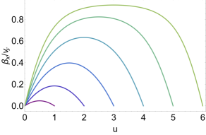
Figure 3: Velocity of the fluid $\beta_{x}$ for the Poiseuille flow as a function of $u$ at different widths $W,$ keeping fixed $\mathcal{E}^{x}=1$, $\mu/k_{B}T=1$. From top to bottom, $w=6,5,4,3,2,1$.

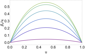
Figure 4: Velocity of the fluid $\beta_{x}$ for the Poiseuille flow as a function of the dimensionless variable $u$ at $\mathcal{E}^{x}=1,w=1$ and different values of $\mu/k_{B}T$. From top to bottom, $\mu/k_{B}T=100,50,20,10,5,1$. If we assume constant $T$, as the density increases, so does the velocity of the fluid.

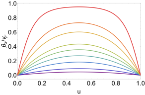
Figure 5: Velocity profile $\beta_{x}$ for the Poiseuille flow as a function of $u$ at different values of $\mathcal{E}^{x}$. From top to bottom: $\mathcal{E}^{x}=50,20,15,10,8,6,4,2,1$. For illustrative purposes, we have taken $w=1$ and $\mu/k_{B}T=1$. Increasing the electric field implies that the fluid velocity increases.

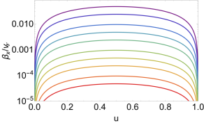
Figure 6: Velocity of the fluid $\beta_{x}$ for the Poiseuille flow as a function of $u$ at different values of the ratio $\eta/s$ while keeping fixed $\mathcal{E}^{x}=1$, $\mu/k_{B}T=1$ and $w=1$. From top to bottom, $4\pi k_{B}\eta/s\hbar=1,2,5,10,20,50,100,200,500,1000$. In order to be able to plot all possibilities, we use a logarithmic scale in the $y$-axis.

• First, from figure 3 we infer that the fluid attains a higher maximal velocity in the middle of the channel as the width $w$ is increased. The reason is that for wider channels, the fluid has more space between the middle of the channel and the boundary, and can transfer a larger total momentum to the walls: In the absence of impurities, the only way for the fluid to lose momentum is to transport it to the boundary via the viscous force between fluid layers. The rate of this momentum transfer between adjacent layers is constant and controlled by $\eta/s$. Hence, integrating (IV.4), losing a larger amount of momentum will need a wider channel. Note that the applicability of our analysis is restricted by the following argument: As in e.g. Molenkamp and de Jong (1994b, a); de Jong and Molenkamp (1995), a cross-over to a ballistic regime is expected if the width of the channel becomes shorter than the electron-electron mean free path $\ell_{\rm ee}=\tau_{\rm ee}v_{F}$. On the other hand, if the width becomes large enough, the maximal velocity in the middle of the channel will be large enough to trigger the onset of turbulent behavior (c.f.  appendix  B for a discussion of the Reynolds number for relativistic flows). Hence the allowed values of $w$ will be restricted to a certain window by these two limits.

• Second, we observe in figure 4 that increasing the chemical potential at fixed temperature, or equivalently decreasing the temperature at fixed chemical potential, leads to an increase of the fluid velocity. This is due to the increase in $\rho/s$ in (IV.4), which governs the coupling between the external electric field and the momentum density. Hence the momentum transfer from the electric field is increased as $\mu/(k_{B}T)$ increases.

• Third, increasing the external electric field $\mathcal{E}^{x}$ increases the velocity of the fluid (see figure 5), since a stronger electric field transfers more momentum to the system.

• Finally, from (IV.4), we see that if $\eta/s$ increases, the kinetic term needs to become smaller in order for the equation to be satisfied at a fixed applied electric field. We confirm this from figure 6, where we display the velocity profile as function of increasing $\eta/s$. We find that strongly coupled fluids move faster than their counterparts at weaker coupling, i.e. at larger $\eta/s$. This is one of the main results of our work.

We now determine the range of values for the parameters $\{\eta/s,\mathcal{E}^{x},\mu/k_{B}T\}$ for which the fluid flows relativistically, i.e. for which the velocity is not small any more compared to the Fermi velocity. From the final point above, we expect the fluid to flow fastest in the strong coupling limit, and hence we take $\eta/s$ to be the holographic value (I.2). From figure 7, we see that at $\mathcal{E}^{x}\simeq 5$ (corresponding to $E_{x}\approx 7.5$ mV/$\mu$m), $\mu/k_{B}T\simeq 0.5$, and the width $w=1$, the velocity becomes about 10% of the Fermi velocity. Hence, for holographic fluids satisfying (I.2), the relativistic regime can be reached for small electric fields and chemical potentials.

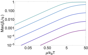
Figure 7: Keeping the ratio $\eta/s$ fixed to $\hbar/4\pi k_{B}$, we plot the maximum speed of the fluid $\beta_{x}$ as a function of the ratio $\mu/k_{B}T$ at different values of the electric field ${\mathcal{E}}^{x}=5,1,0.1,0.01,10^{-3}$. For illustrative purposes, we have set $w=1$. In order to present all possible curves into a single plot, we have employed a logarithmic scale, both on the $x$-axis and $y$-axis. Note also that $\beta_{x}$ never reaches the Fermi velocity $v_{F}$.

IV.2 Momentum relaxation

The wall relaxation time $\tau_{w}$ introduced in sec. III.2 characterizes the rate of momentum outflow through the boundaries. It is expected to be finite due to the finite size $w$ of the channel. Nevertheless, the magnitude of this time-scale relative to the other scales in the problem (c.f. (II.1)) is a priori unclear. In this section we compute $\tau_{w}$ as a function of the input parameters $\mu/k_{B}T,\mathcal{E}_{x},w$ and $\eta/s$ in the absence of impurities. Again, we resort to numerics in order to evaluate (III.15) on the profile solution $\beta_{x}(y)$.

In figure 8 we plot $\tau_{w}$ as a respective function of one of the input parameters $\mu/k_{B}T,\mathcal{E}_{x},w$ and $\eta/s$, while keeping fixed all other input parameters. From these plots, we infer that $\tau_{w}$ is closely related to the speed of the hydrodynamic fluid. Combinations of input parameters that lead to higher velocities will also unavoidably lead to a larger $\tau_{w}$. The underlying reason is that $\tau_{w}$ is a measure for the time needed to lose all the momentum in the flow through the walls. This process naturally takes longer if there is more total momentum in the flow, i.e. if the velocity $\beta_{x}(y)$ is larger. By looking at the slope $\tau_{w}$ as a function of $\eta/s$ in the lower right plot of fig. 8, we find a scaling law of the wall relaxation time as a function of $\eta/s$,

$$\tau_{w}\propto\left(\eta/s\right)^{-1}.$$ (IV.7)

From 8, we see that the typical window of values for $\tau_{w}$ is

$$\tau_{w}\in\left[10^{-9}-10^{-4}\right]\,\rm{s},$$ (IV.8)

We should also point out that what we computed in (III.12) is the instantaneous rate of momentum loss after instantaneously switching off the electric field $E_{x}$. In other words, we assumed that the profile $\beta_{x}(y)$ after switching off the electric field is still the steady state Poiseuille flow. It is expected that the process of momentum loss will slow down as the flow profile $\beta_{x}(y,t)$ evolves non-linearly as a function of time. Hence we expect that the obtained $\tau_{w}$ is a lower bound to the $\tau_{w}$ that would be calculated from solving the time-dependent hydrodynamic equations (II.13) and (II.14).

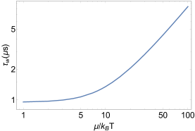
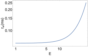
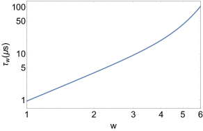
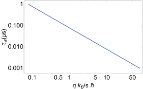
Figure 8: Plot $\tau_{w}$ at different input parameter configurations. Excluding the varying parameter, which varies from plot to plot, we have taken $\mu/k_{B}T=1,\eta/s=\hbar/4\pi k_{B}$, $w=1$, $\mathcal{E}_{x}=1$.

IV.3 Differential wire resistance

In this section we determine the differential wire resistance $\mathcal{R}$, defined by the inverse of the derivative of the current $I$ through the wire with respect to the voltage $V$,

$$\mathcal{R}(I)=\frac{dV}{dI}.$$ (IV.9)

Using (II.11), the total current $I$ that flows across the channel is given by

$$I=\int^{W}_{0}j^{x}(y)dy=\int^{W}_{0}\left[j^{x}_{\rm(fluid)}+j^{x}_{\rm(Q)}\right]dy,$$ (IV.10)

with

$$j^{x}_{\rm(fluid)}=e\rho u^{x},\qquad j^{x}_{\rm(Q)}=\sigma_{Q}\frac{h}{e^{3}c}u_{\alpha}D^{x\alpha}.$$ (IV.11)

From (IV.10) and (III.5), we observe that there are two different types of contributions to $I$: The first contribution, $j^{x}_{\rm(fluid)}\propto u^{x}$, is the flow of the particles along a transverse section of the channel. The second contribution, labeled as $j^{x}_{\rm(Q)}$, is related to the quantum critical conductivity $\sigma_{Q}$ and it accounts for the counterflow of electrons and holes. For the AdS/CFT charged black brane model (A.1), $\sigma_{Q}$ is given by Hartnoll et al. (2007); Hartnoll and Herzog (2007)

$$\sigma_{Q}=\left(\frac{sT}{\varepsilon+p}\right)^{2}\frac{L^{2}}{G_{4}}\frac{e^{2}}{2h}.$$ (IV.12)

For obtaining physical values for the currents, we fix the overall ratio $L^{2}/G_{4}$, where $L$ is the AdS radius $L$ and the Newton constant $G_{4}$, using the AdS/CFT approach described in appendix A. The ratio is fixed to be $L^{2}/G_{4}=64\sqrt{3}$.

Since we apply a constant electric field along the $x$ direction, the voltage is proportional to the applied electric field, $V=E^{x}\,l$, with $l$ the length of the channel, assumed much larger than the width $W$. Both Eqs.(IV.10) and (IV.9) have to be evaluated numerically, since the velocity profile is obtained from a numerical integration. We recast both the $I$ and the differential resistance $\mathcal{R}$ in terms of the reduced variables (IV.1),

$$I =\int\limits^{w}_{0}du\gamma(u)\left[e\rho\beta_{x}(u)+\sigma_{Q}\mathcal{E}^{x}\frac{T^{2}k_{B}^{2}}{ehv_{F}}\right]\,,$$ (IV.13)

$$\mathcal{R} =\frac{ek^{2}_{B}}{h^{2}\epsilon_{0}}\frac{l}{v_{F}^{2}\epsilon_{r}}T^{2}\left(\frac{dI}{d\mathcal{E}^{x}}\right)^{-1}.$$

In sec. IV.1, we focused on deriving the qualitative features of the Poiseuille flow at strong coupling. The aim of this subsection is to obtain a realistic prediction for the value of the resistance. Therefore, we need to use a physically viable combination of input parameters. In experiments, the temperatures are in the range of a few Kelvin Molenkamp and de Jong (1994a, b); de Jong and Molenkamp (1995), whereas the width and length are of order of a few micrometers. We will hereafter assume

$$T=2{\rm K},\quad W=4\mu{\rm m}\quad{\rm and}\quad l=20\mu{\rm m}\,.$$ (IV.14)

The chemical potential can be found from the number density $\rho$ after solving (II.18) for $\mu$. Taking for instance the typical value of the density in experiments, $\rho\simeq 10^{11}\,{\rm cm}^{-2}$, and a spin degeneracy of $g=2$ as well as (IV.14), we find

$$\mu\simeq 4.5\,\text{meV}.$$ (IV.15)

The Fermi velocity and relative permittivity are set according to (IV.2).

In fig. 9 we display the differential resistance as a function of $I$ at different values of the width $W$. It starts with a finite value at $I=0$, and decreases with increasing current until it asymptotes to zero. Increasing the width of the channel leads to a decrease on the differential resistance, as expected for a Poiseuille flow. One might expect that at low $I$, or equivalently $\beta_{x}\ll v_{F}$, the differential resistance should coincide with the quantum critical resistance, $\mathcal{R}_{\rm Q}\sim l/(W\sigma_{Q})$, since at low $I$ there is no macroscopic charge transfer and the wire should act as an Ohmic resistor with an intrinsic conductivity $\sigma_{Q}$ given by (IV.12). However, this expectation does not bear out. Consider the solution for $\beta_{x}$ as obtained from (III.6) restricted to small values of $I$. In this limit the applied electric field must be small and $\beta_{x}\ll v_{F}$. The convection term that appears in the right hand side of (III.6) can be neglected and we obtain a linear differential equation

$$0=h\epsilon_{0}\frac{v_{F}E_{x}\epsilon_{r}\rho}{e\eta}+\beta_{x}^{\prime\prime}(y),$$ (IV.16)

whose solution, consistent also with the boundary conditions (III.4), is given by the usual parabolic profile of the Poiseuille flow

$$\beta_{x}=\frac{\epsilon_{0}h}{e}\frac{E_{x}\epsilon_{r}v_{F}\rho}{2\eta}y(W-y).$$ (IV.17)

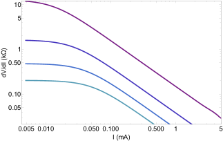
Figure 9: Differential resistance $\mathcal{R}=\frac{dV}{dI}$ as a function of $I$ in absence of impurities and at different widths. From top to bottom (in micrometers), $W=4,3,2,1$. In particular, we have taken $\eta/s=\hbar/4\pi k_{B}$.

Inserting (IV.17) into (IV.10) and integrating over $y$, we obtain the differential resistance

$$\frac{1}{\mathcal{R}}=h\epsilon_{0}\epsilon_{r}v_{F}\frac{W}{l}\left(\frac{\sigma_{Q}}{e^{2}}+\frac{W^{2}\rho^{2}}{12\eta}\right)=\frac{1}{\mathcal{R}_{\rm Q}}+\frac{1}{\mathcal{R}_{\eta}}\,.$$ (IV.18)

Equation (IV.18) contains two contributions of different physical origin: the first comes from the quantum critical resistance $\mathcal{R}_{\rm Q}$, while the second, $\mathcal{R}_{\eta}$, is the viscous resistance generated by viscous effects alone. At fixed chemical potential and temperature, the quantum critical conductance (IV.12) as well as the number density $\rho$ defined in (II.18) are both fixed and

$$\mathcal{R}^{-1}_{\rm Q}\propto W,\qquad\mathcal{R}^{-1}_{\eta}\propto\frac{W^{3}}{\eta}.$$ (IV.19)

Therefore, $\mathcal{R}\simeq\mathcal{R}_{Q}$ only if $W$ is small, or $\eta$ large. Finally, we see that the two contributions to (IV.18) follow an inverse Matthiessen’s rule, i.e.

$$\mathcal{R}^{-1}=\sum\limits_{i=1}^{2}\frac{1}{\mathcal{R}_{i}}\,,$$ (IV.20)

where the $\mathcal{R}_{i}$ are resistances arranged in parallel. The role of $\mathcal{R}_{1}^{-1}$ is played by $\mathcal{R}_{Q}$ and the role of $\mathcal{R}_{2}^{-1}$ is played by $\mathcal{R}_{\eta}$.

The asymptotic form of $\mathcal{R}(I)$ in Fig.9 is related to the asymptotic behavior of $\beta_{x}$ when approaching the Fermi velocity. For large enough electric field, the velocity profile approaches the Fermi velocity, and the first piece of (IV.10) asymptotes to a constant value, while the second contribution is still linear in $E_{x}\propto V$. Taking the derivative with respect to $V$, only the second contribution survives, and the resistance asymptotes to zero due to the $\gamma$ factor. This asymptotic behavior is universal, in the sense that it is not affected by the choice of input parameters within the regime of applicability of hydrodynamics.

We now analyze the dependence of the resistance $\mathcal{R}$ on the viscosity over entropy density ratio $\eta/s$. This provides important information for two reasons: First, as explained in sec. I, $\eta/s$ can be understood as a measure for the coupling strength Fritz et al. (2008); Müller et al. (2009). Second, if the remaining input parameters are known and two different samples are well in the hydrodynamic regime, it will be possible to infer the relative value of $\eta/s$ through a measurement of the wire resistance at small current. This will be of interest from the experimental point of view. In figure 10 we plot the wire resistance $\mathcal{R}$ as a function of the integrated current $I$ at different ratios of $\eta/s$. We find that $dV/dI$ increases with increasing $\eta/s$. This behaviour is related to the decrease of the maximal velocity $\beta_{x}$, and hence of the integral (IV.10), as $\eta/s$ increases.

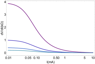
Figure 10: Differential resistance $\mathcal{R}=\frac{dV}{dI}$ as a function of $I$ in absence of impurities. From top to bottom, $k_{B}\eta/s\hbar=5/\pi,5/4\pi,1/2\pi,1/4\pi$.

V Flow and differential resistance in the presence of impurities

We now examine the effect of impurities on the results of section IV, as is essential in view of comparison with experiments. In this case, the AdS/CFT results (II.18) are no longer directly applicable since the pressure becomes $y$-dependent, as given by (III.7) for finite $\tau_{\mathrm{imp}}$. In the non-relativistic limit, however, where $\gamma\rightarrow 1$, this $y$-dependence drops out again from all the thermodynamic variables.

We thus consider the non-relativistic limit in this section. This restricts us to small values of the applied electric field. On the other hand, we are able to obtain analytical results in this regime, and to perform a general hydrodynamical analysis applicable to any value of the electron-electron coupling.

V.1 Velocity profiles

We begin by examining the velocity profile of the fluid. As discussed above, we consider the non-relativistic limit, in which the non-linear terms that enter the Navier-Stokes equations (III.6) are suppressed and it is possible to find an analytic solution for $\beta_{x}$. Linearizing (III.6) in $\beta_{x}$ gives

$$\frac{\eta}{s}\beta_{x}^{\prime\prime}+E_{x}\epsilon_{r}v_{F}\frac{\rho}{s}\left(\frac{h\epsilon_{0}}{e}\right)-\frac{\beta_{x}}{\tau_{\rm imp}v_{F}^{2}}\frac{\varepsilon+p}{s}=0.$$ (V.1)

Imposing $\beta_{x}(0)=\beta_{x}(W)=0$, we obtain the profile as a function of the $y$ coordinate,

$$\beta_{x}(y) =v_{F}\epsilon_{r}\frac{E_{x}h\epsilon_{0}}{e}\frac{\rho}{\eta\mathcal{G}^{2}}$$

$$\times \left[1-\cosh\left(\mathcal{G}y\right)+\sinh\left(\mathcal{G}y\right)\tanh\left(\frac{\mathcal{G}W}{2}\right)\right],$$ (V.2)

with

$$\mathcal{G}=\frac{1}{v_{F}}\sqrt{\frac{\varepsilon+p}{\eta\tau_{\rm imp}}},\qquad\left[\mathcal{G}\right]={\rm m}^{-1}.$$ (V.3)

Note that the result for the velocity profile is analytical in the limit considered here, while the relativistic result of the preceding section is numerical. We also note that $\beta_{x}$ as given by (V.1) reduces to the parabolic flow (IV.17) in the limit $\tau_{\rm imp}\to\infty$, as expected. In Fig. 11, we display the velocity profile of (V.1) as function of the impurity scattering time. We observe that when increasing the impurity density while keeping all other input parameters fixed, the velocity decreases.

If the density of impurities is such that $\tau_{\rm imp}$ becomes the shortest time scale of the system, shorter than the electron-electron scattering time, then impurity collision effects are dominant. In this case, the Poiseuille hydrodynamic behavior is suppressed and a standard Ohmic conductivity law is expected instead. Indeed, the Poiseuille flow connects smoothly to an Ohmic regime as may be seen as follows. We consider the non-relativistic limit of (III.6) and assume that $\eta/s\ll T\tau_{\rm imp}$. Then

$$\beta_{x}=\frac{v_{F}^{3}\tau_{\rm imp}\epsilon_{r}\epsilon_{0}h}{e(\varepsilon+P)}\rho E_{x}\,.$$ (V.4)

Inserting this expression in $j_{x}=e\rho\beta_{x}+\sigma_{Q}E_{x}$, we obtain in the non-relativistic limit

$$j_{x}=\left(\sigma_{Q}+\rho^{2}\frac{v_{F}^{3}\tau_{\rm imp}\epsilon_{r}\epsilon_{0}h}{\varepsilon+P}\right)E_{x}=\left(\sigma_{Q}+\sigma_{D}\right)E_{x}\,.$$ (V.5)

The overall conductivity $\sigma$ consists of the sum of the quantum critical conductivity $\sigma_{Q}$ and the Drude conductivity $\sigma_{D}$, given by

$$\sigma_{D}=\rho^{2}\frac{v_{F}^{3}\tau_{\rm imp}\epsilon_{r}\epsilon_{0}h}{\varepsilon+P}\,.$$ (V.6)

From the quantum critical conductivity defined in (IV.12) and for a typical value of $\tau_{\rm imp}=10^{-12}$s de Jong and Molenkamp (1995), we find that

$$\frac{\sigma_{D}}{\sigma_{Q}}=\frac{\rho_{Q}}{\rho_{D}}\simeq 0.84$$ (V.7)

for the input parameters given around (IV.2) and (IV.15). This implies that the quantum critical conductivity plays a more significant role in the current $j^{x}$ of (V.5), although both are of the same order of magnitude. This shows that at strong coupling, the electron-hole scattering effect that gives rise to the quantum critical conductivity Fritz et al. (2008) cannot be neglected compared to impurity scattering: At weak coupling, Fritz et al. (2008) the quantum critical resistivity drops to zero as $\alpha^{2}(T)$ and the Drude resistivity is expected to approach a constant. At strong coupling on the other hand Fritz et al. (2008), the quantum critical resistivity is expected to saturate as well, to a universal value $\sim\frac{h}{e^{2}}$. Hence, while at weak coupling the ratio (V.7) is expected to approach zero, it is expected to asymptote to a constant for strongly interacting electron systems. We will further elaborate on the differences of strong and weakly coupled electron systems in sec. VII.

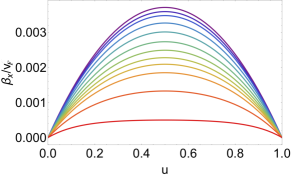
Figure 11: Velocity profile $\beta_{x}$ along the $x$ direction, $\beta_{x}(u)$, at different mean free time $\tau_{\rm imp}$. From top to bottom: $T\tau_{\rm imp}k_{B}/h=10^{4},20,10,5,3,2,1.5,1.2,1,0.8,0.5,0.2$. It is remarkable to notice that for the lowest curve, the profile is almost zero in the interior. For all the curves, we have set $\mu/k_{B}T=1$, $\eta/s=\hbar/4\pi k_{B}$ and $\mathcal{E}^{x}=w=1$.

In conclusion, we observe that when increasing the impurity density while keeping all other input parameters fixed, the fluid velocity decreases. Moreover, if $\tau_{\rm imp}<\tau_{\rm ee}$, the flow will no longer be of Poiseuille form, since the impurities absorb momentum. If the density of impurities is large enough, impurity effects dominate and the electron flow becomes Ohmic. Since the transition between the Poiseuille and Ohmic flows is determined by the interplay of two scales, the electron-electron scattering rate and the impurity scattering rate, this transition is a cross-over.

V.2 Momentum relaxation

Here we calculate the wall relaxation time $\tau_{w}$ within hydrodynamics for the Poiseuille flow V.1. The result is valid for any value of the electron-electron coupling. This is particularly interesting from the AdS/CFT point of view since wall momentum relaxation has not yet been analyzed in this context. Moreover, we aim at retrieving the physics associated to the interplay of impurity and finite size effects, both of relevance in experiments.

Since the velocity profile $\beta_{x}$ of (V.1) is known analytically, $\tau_{w}$ may also be computed analytically. We expand (III.15) at small $\beta_{x}$,

$$\int^{W}_{0}dy\,\frac{\beta_{x}}{v_{F}}\left(p+\varepsilon\right)\left(\frac{1}{\tau_{w}}+\frac{1}{\tau_{\rm imp}}\right)=\eta\left.\beta^{\prime}_{x}(y)\right|_{y=W}^{y=0},$$ (V.8)

and insert the solution (V.1) into (V.8) to find

$$\tau_{w}=\frac{\tau_{\rm imp}}{2}\left[\frac{W\mathcal{G}}{4\tanh\left(\frac{W\mathcal{G}}{2}\right)-W\mathcal{G}}-1\right].$$ (V.9)

As we see from (V.3), $\mathcal{G}$ is an involved function of the thermodynamic variables, the shear viscosity $\eta$ and the impurity scattering rate $\tau_{\rm imp}$.

For a fluid propagating through the channel, we expect that the wall momentum relaxation time is larger in presence than in absence of impurities, $\tau_{w}^{(\tau_{\rm imp}<\infty)}>\tau_{w}^{(\tau_{\rm imp}\to\infty)}$. This is due to impurity momentum relaxation competing with wall momentum absorption. Indeed, if we consider a small density of impurities or equivalently large $\tau_{\rm imp}$, we find from expanding (V.9) that the wall relaxation time in the presence of impurities is always longer than in a completely clean sample,

$$\tau_{w}^{(\tau_{\rm imp}<\infty)} \simeq\tau_{w}^{(\tau_{\rm imp}\to\infty)}$$

$$+\frac{W^{2}}{180\tau_{\rm imp}v_{F}^{4}}\left[\frac{W^{2}(p+\epsilon)^{2}}{\eta^{2}}+15v_{F}^{2}\right]\,,$$ (V.10)

with

$$\tau_{w}^{(\tau_{\rm imp}\to\infty)}=\frac{W^{2}(p+\epsilon)}{12\eta\,v_{F}^{2}}.$$ (V.11)

In particular, after using the Gibbs-Duhem relation (II.20),

$$\tau_{w}^{(\tau_{\rm imp}\to\infty)}=\frac{W^{2}}{12\eta\,v_{F}^{2}}\left(\mu\frac{\rho}{\eta}+T\frac{s}{\eta}\right),$$ (V.12)

we can confirm analytically the $(\eta/s)^{-1}$ scaling dependence in the relaxation time through the walls, as it was firstly predicted in Sec.V.2. Notice however that no physical reasons a priori state why this scaling dependence is preserved in the ultra-relativistic regime ($\beta_{x}\simeq v_{F}$), rendering thus the fully-fledged analysis of the Navier-Stokes equation (IV.4) of great relevance.

In addition, from the balance equation (III.15), we see that the r.h.s. is determined by the velocity profile at fixed $\eta$, whereas the l.h.s. is proportional to the sum of $\tau_{w}^{-1}$ and $\tau_{\rm imp}^{-1}$. Therefore, for a fixed velocity profile $\beta_{x}$, $\tau_{w}$ becomes larger if $\tau_{\rm imp}$ decreases. Equivalently, momentum diffusion through the boundaries is impeded by the presence of impurities, even though both mechanisms lead to momentum absorption.

V.3 Differential resistance

Finally we compute the differential resistance of our channel in the presence of impurities. We use again the same formulae for the current and differential resistance, (IV.10) and (IV.9). As before, for a constant energy density even in the presence of impurities, we have to consider the non-relativistic limit. This in turn leads to analytical results.

We insert the velocity profile (V.1) into the current (IV.10) and find

$$I=\frac{V}{l}v_{F}\epsilon_{r}\left(h\epsilon_{0}\right)\Bigg{\{}\frac{W}{e^{2}}\sigma_{Q}+\frac{\rho^{2}}{\mathcal{G}^{3}\eta}\left[W\mathcal{G}-2\tanh\left(\frac{W\mathcal{G}}{2}\right)\right]\Bigg{\}}\,.$$ (V.13)

Here, $W$ is the dimensionful width of the channel, $l$ is its length, $\mathcal{G}$ is given by (V.3), $\sigma_{Q}$ is the quantum critical conductivity, $\rho$ is the number density and $\eta$ the shear viscosity. (V.13) is linear in $V$, so that

$$\mathcal{R}^{-1}=\frac{I}{V} =v_{F}h\epsilon_{0}\epsilon_{r}\frac{1}{l}\times$$

$$\times\Bigg{\{}\frac{W}{e^{2}}\sigma_{Q} +\frac{\rho^{2}}{\mathcal{G}^{3}\eta}\left[W\mathcal{G}-2\tanh\left(\frac{W\mathcal{G}}{2}\right)\right]\Bigg{\}}.$$ (V.14)

The differential resistance $\mathcal{R}$ given by (V.3) is independent of the current $I$. This follows from the non-relativistic limit in which $I$ is linear in $V\propto E_{x}$. Terms of higher order in $E^{x}$ contributing to the equations of motion (V.1) and to the velocity profile solution (V.1) would signal relativistic effects, as we may see from the analysis of the velocity profile when impurities are absent (Fig.7). This means that the relation between the current $I$ and the quantities on the r.h.s. of (V.13) is valid only for small current $I$, in consistency with the approximation of small $E_{x}$. Nevertheless, (V.13) can be used to predict the value of the maximum of the differential resistance in a hydrodynamic Poiseuille flow once the input parameters and thermodynamic variables are fixed.

Viscous and impurity effects cannot be disentangled in the expression for $\mathcal{R}$ (recall that $\mathcal{G}$, given by (V.3), in (V.3), depends both on $\eta$ and $\tau_{\rm imp}$). This follows from the fact that the $j^{x}_{\rm(fluid)}$ contribution to the current density (IV.11) inherits a non-trivial dependence on $\eta$ and $\tau_{\rm imp}$ from the velocity profile (V.1). Viscous and impurity effects may not even be disentangled in the limit of vanishing $\tau_{\mathrm{imp}}\rightarrow\infty$. This may be seen by expanding (V.3) at large $\tau_{\rm imp}$,

$$\mathcal{R}^{-1}_{(\tau_{\rm imp}<\infty)} \sim \mathcal{R}^{-1}_{(\tau_{\rm imp}\to\infty)}-\frac{W^{5}}{120\eta^{2}\tau_{\rm imp}}\frac{h}{v_{F}\,l}\epsilon_{0}\epsilon_{r}\rho^{2}(p+\varepsilon)$$ (V.15)

$$\sim \mathcal{R}^{-1}_{(\tau_{\rm imp}\to\infty)}$$

$$- \frac{W^{5}}{120\eta\tau_{\rm imp}}\frac{h}{v_{F}\,l}\epsilon_{0}\epsilon_{r}\rho^{2}\left(T\frac{s}{\eta}+\mu\frac{\rho}{\eta}\right),$$

with $\mathcal{R}^{-1}_{(\tau_{\rm imp}\to\infty)}$ as defined in (IV.18). The second piece on the left-hand side of (V.15) depends not only $\eta$ and $\tau_{\rm imp}$, but also on the ratio $\eta/s$. Nevertheless, laboratory samples usually have a significant impurity density, implying that $\tau_{\rm imp}$ can be rather small. Expanding (V.3) at low $\ell_{\rm imp}$ compared to the width of the channel $W$, we find

$$\mathcal{R}^{-1}\sim\mathcal{R}^{-1}_{Q}+\mathcal{R}^{-1}_{\eta},$$ (V.16)

with $\mathcal{R}^{-1}_{Q}$ the quantum critical resistance as defined in IV.18, and this time, $\mathcal{R}^{-1}_{\eta}$ defined by

$$\mathcal{R}^{-1}_{\eta}=\sigma_{D}-\mathcal{R}^{-1}_{(1)}+\cdots,$$ (V.17)

with $\sigma_{D}$ the Drude conductivity, defined in V.6 and

$$\mathcal{R}^{-1}_{(1)}=2E_{x}h\rho^{2}v_{F}^{4}\epsilon_{r}\epsilon_{0}\tau_{\rm imp}\left[\frac{\tanh\left(\frac{\mathcal{G}W}{2}\right)}{\varepsilon+p}\right]\sqrt{\frac{\tau_{\rm imp}\eta}{\mu\rho+sT}},$$ (V.18)

which in particular depends on the ratio $\eta/s$. This last term, despite of being subleading with respect to the Drude conductivity, its contribution can be significant enough to be accounted for. Indeed, for the set of input parameters IV.2, IV.14 and IV.15, the relative difference $\xi$ between $\mathcal{R}^{-1}_{(1)}$ and $\sigma_{D}$ is found to be

$$\xi=\Big{|}\frac{\sigma_{D}-\mathcal{R}^{-1}_{(1)}}{\sigma_{D}}\Bigg{|}\sim 0.9,$$ (V.19)

for $\tau_{\rm imp}\sim 10^{-11}$s. This relative difference becomes even smaller ($\xi\to 0$) for cleaner samples. Given the fact that $\mathcal{R}^{-1}_{(1)}$ depends significantly on $\eta/s$ and hence on the coupling, one can state that for cleaner samples, it is expected to experimentally observe significant departures from the hydrodynamical differential resistance with respect to the $\mathcal{R}_{\eta}\propto\eta$ law found in the literature. This prediction is complementary to the analysis at zero impurities carried out in section IV, where we showed that the differential resistance highly depends on $\eta/s$.

VI Reynolds Number for Channel Flows

One of the main results of this work is that strongly coupled fluids flow fastest. For sufficiently large fluid velocities, the fluid can become turbulent. Between the laminar regime and fully developed turbulence, there is a transitional preturbulent regime in which both laminar and turbulent flows coexist. The Reynolds number $Re$ is used to quantitatively determine the transition between laminar and turbulent flows. In appendix B, we provide a derivation of the Reynolds number, both for ultra-relativistic and non-relativistic viscous fluids. The non-relativistic Reynolds number is shown in (B.4). For Newtonian fluids moving through a 2+1-dimensional channel, a Reynolds number $Re<100$ is associated with clearly laminar flows, while highly turbulent flows occur for $Re\gg 100$ Hanks (1963, 1969). Using the KSS bound for $\eta/s$ (I.3), an upper bound on the Reynolds number (B.4),

$$Re\leq\frac{4\pi k_{B}}{\hbar}\frac{\left(\varepsilon+p\right)W}{sv_{\rm max}}\left(\frac{v_{\rm max}}{v_{F}}\right)^{2},$$ (VI.1)

can be derived. Based on this, for the same maximal flow velocity $v_{\rm max}$ and width $W$, it is reasonable to assume that a strongly coupled fluid is more likely to become turbulent than its weakly coupled counterpart. From (II.18), in the near Fermi liquid limit we obtain

$$\frac{\varepsilon+p}{s}\Bigg{|}_{\mu\gg k_{B}T}=\frac{\sqrt{3}}{16\pi}\frac{\mu}{k_{B}}.$$ (VI.2)

Hence, large chemical potentials enhance the transition to the turbulent regime. Estimating the right hand side of (VI.1) with input parameters (IV.14)-(IV.15), we find $Re\leq 50$. Therefore, for our channel widths, the flow is clearly laminar Hanks (1963, 1969), but if wider channels could be synthesized in the hydrodynamic regime, higher Reynolds numbers can be achieved since $Re\propto W$. Also, following Mendoza et al. (2011), inserting an obstacle into the channel or considering flows through a constriction may allow for preturbulent physics such as vortex shedding.

However, impurities should be accounted for in this analysis. We can accomplish this by introducing the Gurzhi length $\lambda_{G}$, Lucas and Fong (2017) defined as

$$\lambda_{G}=v_{F}\sqrt{\kappa\tau_{\rm imp}},\qquad\kappa=\frac{\eta}{\varepsilon+p}.$$ (VI.3)

where $\kappa$ is the kinematic viscosity of the fluid.Using $\lambda_{G}$ we may define two inequivalent regimes: First, if $W<\lambda_{G}$, it is likely that the fluid will propagate according to a Poiseuille flow, with a large speed in the middle of the channel. By using the definition of Reynolds number in the ultra-relativistic limit (B.6) derived in appendix B, we find

$$Re_{(W<\lambda_{G})}=\frac{\tau_{\rm imp}v_{F}}{W}\left(\frac{W}{\lambda_{G}}\right)^{2}\left(\frac{v_{F}}{v_{\rm max}}\right)^{3}.$$ (VI.4)

Notice that the condition $W<\lambda_{G}$ introduces a bound on $\tau_{\rm imp}$. This bound is given by

$$\tau_{\rm imp}>\frac{W^{2}}{v_{F}^{2}\kappa}.$$ (VI.5)

Since $v_{\rm max}\leq v_{F}$, even though they are of similar magnitude, using (VI.5) we find that the Reynolds number is bounded from below by

$$Re>\frac{W}{v_{F}\kappa}\left(\frac{W}{\lambda_{G}}\right)^{2}.$$ (VI.6)

Second, when $W>\lambda_{G}$, the fluid motion signals the onset of an Ohmic flow although the no-slip conditions at the boundary are still satisfied. Qualitatively speaking, instead of a Poiseuille-type velocity profile, one should expect a plateau around the middle of the channel. We can confirm this behavior from Fig.11, wherein we plotted $\beta_{x}$ at different $\lambda_{G}$ (mind that $\eta$, the temperature and the chemical potential were fixed, which fixes $\kappa$). We expect the fluid velocity not to be large, $v_{\rm max}\ll v_{F}$, in the $W>\lambda_{G}$ regime. The condition $W>\lambda_{G}$ is translated then into an upper bound for the impurity scattering rate

$$\tau_{\rm imp}<\frac{W^{2}}{v_{F}^{2}\kappa}.$$ (VI.7)

The (non-relativistic) Reynolds number in this case is given by

$$Re_{(W>\lambda_{G})}=\frac{2}{3}\frac{v_{F}\tau_{\rm imp}}{W}\left(\frac{W}{\lambda_{G}}\right)^{2}\frac{v_{\rm max}}{v_{F}}.$$ (VI.8)

Inserting (VI.7) and (VI.3) into (VI.8), we see that the Reynolds number is bounded from above. The bound is given by

$$Re<\frac{2}{3}\frac{W}{v_{F}\kappa}\left(\frac{W}{\lambda_{G}}\right)^{2}\frac{v_{\rm max}}{v_{F}}.$$ (VI.9)

It is also worthwhile to mention that

$$Re_{(W<\lambda_{G})}>Re_{(W>\lambda_{G})},$$ (VI.10)

since $\tau_{\rm imp}$ when $W<\lambda_{G}$ needs to be large for consistency. Based on this last result (VI.10), we can conclude that the onset of turbulence is more likely to appear in clean samples.

VII Discussion and outlook

In this work, we considered the motion of relativistic strongly coupled electron fluids propagating along a channel under an applied electric field. Due to the incompressibility of the flow as well as the expected near-conformality of relativistic electron systems such as graphene Novoselov et al. (2005) or HgTe König et al. (2007), transport is characterized by a single transport coefficient, the ratio of shear viscosity to entropy density $\eta/s$. We analyzed the qualitative dependence of the fluid flow on $\eta/s$ in relativistic clean systems in sec. IV, and the non-relativistic case with momentum relaxation in sec. V. In a phenomenological approach, we varied $\eta/s$ from its strong coupling value (I.2) predicted by AdS/CFT towards the intermediate coupling regime in which $\eta/s$ is larger Müller et al. (2009). We generically find that keeping the other input parameters such as e.g. electric field and impurities fixed, strongly coupled holographic fluids satisfying (I.2) flow fastest.

A very important observable for hydrodynamic behavior in such channels, also called high-mobility wires, is the differential resistance. It is sensitive to the ballistic-to-hydrodynamic crossover Molenkamp and de Jong (1994a, b); de Jong and Molenkamp (1995). Our hydrodynamic simulations show that the differential resistance has the form expected for a Poiseuille flow, and depends sensitively on the value of $\eta/s$. In particular, we found that the differential resistance becomes minimal for strongly coupled fluids satisfying (I.2). This is due to the dependence of the current defined in (IV.10) on the velocity profile, which, as can be seen from Fig. 6, itself depends strongly on $\eta/s$. Thus, keeping all other parameters fixed, we expect the holographic fluids to exhibit the smallest resistance. From the qualitative behavior of the channel resistance $dV/dI$ as a function of $\eta/s$ obtained from our hydrodynamic simulations (c.f. Fig. 10) we conclude that if the equilibration length associated with (I.1) is of the order of the channel width $w$, the position of the Gurzhi maximum indicative of the Knudsen-Poiseuille crossover strongly depends on $\eta/s$.

Moreover, we calculated the wall momentum-relaxation timescale $\tau_{w}$, which describes how fast momentum is lost through the walls. We found it to be largest for holographic fluids. We interpret this as follows: The shear viscosity $\eta$ is a measure of the momentum transfer between adjacent fluid layers. The entropy density $s$ is a measure of the number of degrees of freedom in each layer, at a given temperature and chemical potential. Hence, $\eta/s$ can be interpreted as the rate of momentum transfer between adjacent fluid layers per effective degree of freedom. This implies that the momentum transfer between layers is less efficient for small $\eta/s$ and hence $\tau_{w}$ is larger in this case. Note also that $\eta/s$ is related to the relativistic analogue of the kinematic viscosity by means of the Gibbs-Duhem relation (II.20).

Furthermore, we found that boundary-induced momentum relaxation is not independent of momentum loss through impurities: Decreasing the impurity density leads to an increased total momentum of the flow, which in turn decreases wall momentum relaxation (c.f. (V.8)). We derived the exact relationship between wall momentum relaxation $\tau_{w}$ and impurity momentum relaxation $\tau_{\rm imp}$ for non-relativistic flows in (V.9). Experimentally verifying the consequences of wall momentum relaxation requires to synthesize clean enough samples with small $\eta/s$ such that $\tau_{w}$ is comparable to $\tau_{\rm imp}$ (c.f. (IV.8)).

In the nonrelativistic limit we derived a closed form for the differential resistance $\mathcal{R}$, given in (V.3). For all other input parameters held fixed, $\mathcal{R}$ is a monotonically decreasing function of $\tau_{\rm imp}$, as expected. We stress that the expression (V.3) for $\mathcal{R}$ is only valid for small values of the current $I$. Therefore, provided that the system behaves hydrodynamically, (V.3) gives the maximal resistance of the channel. In the present work, we have assumed that the system is well in the hydrodynamic regime (II.1). In addition, we found that $\mathcal{R}$ satisfies an inverse Matthiessen’s rule, which in the absence of impurities is given by (IV.18). In the presence of impurities, $\mathcal{R}_{\eta}^{-1}$ in (IV.18) is replaced by the second term in (V.3). From (IV.18) and its expansion around the clean limit (V.15), quantum critical conductance effects are separable from viscous and impurity effects in the way how they enter (V.3). The underlying reason is that in the constitutive relation for the current (II.11), they enter as two independent terms. This will also hold for flows with other boundary conditions.Kiselev and Schmalian (2018) This is reminiscent of situations in AdS/CFT models of strange metallic physics, where the quantum critical part and the Drude part of the conductivity also follow an inverse Matthiessen rule Goutéraux (2014), or even more nonlinear relations. Karch and O’Bannon (2007) We emphasize that the expression (V.3) for the wire resistance was derived without any particular assumption about the equation of state or the value of $\eta/s$. It is hence valid at weak coupling as well, as long as the conditions for hydrodynamics (II.1) apply.

Throughout our calculations, we used the expression (IV.12) for the quantum critical conductivity $\sigma_{Q}$. This choice is most natural at strong coupling for the following reason: The quantum critical conductivity can be calculated at weak coupling Fritz et al. (2008) to leading order in $\alpha(T)$. The result is similar to (I.4) for $\eta/s$,

$$\sigma_{Q}=0.76\frac{e^{2}}{h}\frac{1}{\alpha^{2}(T)}.$$ (VII.1)

Following the discussion of $\eta/s$ in sec. I and extrapolating this result to strong coupling, the natural value for the quantum critical conductivity at strong coupling is of order

$$\sigma_{Q}\sim\frac{e^{2}}{h}\,.$$ (VII.2)

From (V.7) we see that at strong coupling, the quantum critical resistivity is of the same order as the Drude resistivity for realistic values of the impurity density. Hence, the quantum critical part of the resistivity cannot be neglected, contrary to the situation at weak coupling. The normalization of the $F^{2}$ term in our holographic model (A.1) was chosen to bear out this expectationHartnoll et al. (2007); Hartnoll and Herzog (2007) to yield (IV.12).

In view of the discussion on the onset of turbulence in sec. VI, it will be highly interesting to perform fully space-time dependent hydrodynamic simulations in 2+1 dimensional charged fluids. This is also interesting from the point of view of the viscosity and impurity induced pressure drop (III.9) found as a solution to the Hagen-Poiseuille equation (III.7). The classical Hagen-Poiseuille law relates the pressure drop along a laminar flow in a pipe, in our case the wire, to the viscosity of the flowing fluid. This effect is present as long as the viscosity is non-vanishing, independently of the presence of impurities. If we allow for $x$-dependence in our hydrodynamic simulations, we will recover that well-known effect, as well as (III.9). In any fluid, pressure gradients translate into gradients in energy density via the equation of state $\epsilon(p)$, and hence into a spatially dependent temperature. It will be very interesting to investigate this and other space-time dependent effects further.

Another interesting question is the physical significance of the relative ordering of the channel with $W$ versus the impurity mean free path $\ell_{\rm imp}$ in (II.1). The relevant length scale to compare $W$ to is the Gurzhi length $\lambda_{G}=v_{F}\sqrt{\kappa\tau_{\rm imp}}$, with $\kappa$ the kinematic viscosity. The Gurzhi length is the scale on which the viscous drag in the channel is efficient. Lucas and Fong (2017) In the Poiseuille regime $W\leq\lambda$, the viscous drag from the boundaries permeates the entire channel. In the opposite regime $W\geq\lambda$, the viscous drag is important up to a distance of order $\lambda_{G}$ away from the walls, but in the center of the channel, the physics is effectively 2+1-dimensional, and the flow is Ohmic. The latter point is noteworthy as it represents an Ohmic electric response in the regime of applicability of hydrodynamics (II.1).

The results presented in this work assume the validity of hydrodynamics (II.1) at all electron temperatures and input parameters. The hydrodynamic regime is reached if the electron-electron mean free path $\ell_{\rm ee}$ is the smallest length scale present. This is expected to be the case in particular in systems with strong electron-electron correlations. Realizing such strongly correlated electron systems will hence be an important avenue for further development. The above considerations about the applicability of hydrodynamics may not however apply at intermediate coupling strengths. There, new non-hydrodynamic modes may appear, invalidating the hydrodynamic expansion, as was explained in footnote 48. One possible approach for investigating whether hydrodynamics remains applicable at intermediate couplings is to study gravitational duals at finite charge density that include coupling corrections.Anninos and Pastras (2009)Witczak-Krempa and Sachdev (2012)Witczak-Krempa and Sachdev (2013)Grozdanov and Starinets (2017)Gross and Sloan (1987)

Finally, it will be interesting to investigate the effect of parity and time reversal breakingJensen et al. (2012); Hoyos (2014); Pellegrino et al. (2017); Delacretaz and Gromov (2017) in the setup considered, as well as thermal and thermoelectric transport.

Appendix A Holographic set-up

Here we review some aspects of the AdS/CFT correspondence relevant to our analysis and fix the overall coefficient of the gravity action. Since we are interested in planar 2+1 dimensional systems, we will work in 3+1 bulk dimensions, i.e. consider a gravity model with an AdS₄ ground state.

The simplest holographic set-up which accommodates matter at finite charge density and temperature is the field theory dual to Einstein-Maxwell theory,

$$S=\frac{1}{16\pi G_{4}}\int\,d^{4}x\sqrt{-g}\left[R-2\Lambda-L^{2}F_{\mu\nu}F^{\mu\nu}\right]\,.$$ (A.1)

Here $R$ is the Ricci curvature scalar, $\Lambda=-\frac{3}{L^{2}}$ is the negative cosmological constant necessary to generate an Anti de Sitter space-time of curvature radius $L$ as the ground state of (A.1), and $F_{\mu\nu}=\partial_{\mu}A_{\nu}-\partial_{\nu}A_{\mu}$ the field strength for the $U(1)$ gauge connection $A_{\mu}$. Turning on a dynamical $U(1)$ gauge field allows for a QFT at finite density. In particular, we consider

$$A_{\mu}dx^{\mu}=A_{0}dt.$$ (A.2)

The chemical potential is defined as the boundary value of the time component of the bulk gauge $U(1)$ field,

$$\mu=A_{0}(r)\big{|}_{r\to\infty}.$$ (A.3)

In order to describe a QFT at non-zero temperature, we need to consider a black brane in the gravity dual. The reason is that the Hawking temperature $T_{H}$ of the black brane is identified with the temperature of the QFT, $T=T_{H}$. To this purpose, we consider the line element of the AdS-Reissner-Nordström black brane, given by

$$ds^{2}=\frac{L^{2}}{r^{2}f(r)}dr^{2}+\frac{r^{2}}{L^{2}}\left[-f(r)v_{F}^{2}dt^{2}+dx^{2}\right]\,.$$ (A.4)

The black brane encloses a charge density inside the horizon, sourcing a Coulomb potential $A_{N}dx^{N}=A_{0}(r)dx^{0}$ varying in the holographic direction $r$. The emblackening factor $f(r)$ and Coulomb potential $A_{0}(r)$ are

$$f(r) = 1-\frac{r_{H}^{3}}{r^{3}}-\frac{1}{4}\frac{\mu^{2}L^{4}}{\hbar^{2}v_{F}^{2}}\frac{r_{H}}{r^{3}}\left[1-\frac{r_{H}}{r}\right]\,,$$

$$A_{0} = \frac{\mu}{\hbar v_{F}}\left(1-\frac{r_{H}}{r}\right).$$ (A.5)

The Hawking temperature is obtained from the surface gravity $\kappa_{H}$, defined as

$$2\pi\frac{v_{F}\,k_{B}}{\hbar}T_{H}=\kappa_{H}=\sqrt{\Big{|}\left(\nabla_{A}\zeta_{B}\right)\left(\nabla^{A}\zeta^{B}\right)\Big{|}}\Bigg{|}_{r=r_{H}}.$$ (A.6)

For a static black brane, one Killing vector is simply $\zeta=\left(\zeta^{r},\zeta^{t},\zeta^{x},\zeta^{y}\right)=(0,1,0,0)$. $\nabla_{a}$ stands for the covariant derivative, defined from the bulk metric (A.4). With this,

$$T_{H}=\frac{\hbar\,v_{F}}{k_{B}}\frac{r_{H}}{4\pi L^{2}}f^{\prime}(r_{H})e^{A(r_{H})},$$ (A.7)

which, for the functions defined in (A.5), gives

$$T_{H}=\frac{1}{\hbar\,v_{F}k_{B}}\frac{\mu^{2}L^{2}}{16\pi r_{H}}-\frac{\hbar v_{F}}{k_{B}}\frac{3r_{H}}{4\pi L^{2}}.$$ (A.8)

Notice that due to the horizon, the radial coordinate spans from the horizon position $r_{H}$ to the boundary, that is $r\in[r_{H},\infty]$. The metric (A.4) asymptotes to an $\rm{AdS}_{4}$ space of radius $L$ for $r\to\infty$. Since our aim is to describe a hydrodynamic fluid of relativistic electrons, the Fermi velocity $v_{F}$ replaces the vacuum speed of light $c$. The position of the event horizon $r_{H}$ is fixed in terms of the chemical potential and the Hawking temperature,

$$\frac{r_{H}}{L^{2}}=\frac{1}{6}\frac{k_{B}T}{\hbar\,v_{F}}\left(4\pi+\sqrt{16\pi^{2}+\frac{3\mu^{2}}{k_{B}^{2}T^{2}}}\right).$$ (A.9)

The entropy density of the QFT is identified with the Bekenstein-Hawking entropy density, which is given by

$$s=\frac{\mathcal{A}_{H}\,k_{B}}{4l_{*}^{2}},\qquad l_{*}^{2}=\frac{\hbar G_{4}}{v_{F}^{3}}.$$ (A.10)

The area density, $\mathcal{A}_{H}$, is

$$\mathcal{A}_{H}=\sqrt{g_{xx}g_{yy}}\big{|}_{r\to r_{H}}.$$ (A.11)

For the metric element (A.4), we get

$$\mathcal{A}_{H}=\frac{r_{H}^{2}}{L^{2}}.$$ (A.12)

A finite density in the dual QFT is obtained by turning on a dynamical $U(1)$ gauge field,

$$A_{\mu}dx^{\mu}=A_{0}dt.$$ (A.13)

There is a non-trivial relation between the bulk fields $f$ and $A_{0}$ and the chemical potential and temperature. The chemical potential is defined as the boundary value of the time component of the bulk gauge $U(1)$ field,

$$\mu=A_{0}(r)\big{|}_{r\to\infty}.$$ (A.14)

Having identified the temperature and chemical potential, we now proceed to determine the thermodynamical variables that appear in (II.18), with the exception of the entropy density, already defined in (A.10). The holographic duality establishes that the partition function of the QFT and of the gravity theory are identified. Taking variations of the on-shell gravity action (A.1) with respect to the metric or the gauge field will give the corresponding $n$-point correlation functions. The on-shell action is divergent and we need to renormalize it. This constitutes the holographic renormalization prescription de Haro et al. (2001); Papadimitriou and Skenderis (2004, 2005). We introduce a cutoff in the radial direction $r_{\Lambda}$ such that the divergences of the bulk action (A.1) are regulated. The volume divergence is canceled by adding the counterterm

$$S_{c.t.}=-\frac{1}{16\pi G_{4}}\int_{r=r_{\Lambda}}d^{3}x\,{\cal L}_{c.t.},\quad{\cal L}_{c.t.}=\sqrt{-\gamma}\frac{6}{L}\ .$$ (A.15)

Further divergences, subleading with respect to the volume divergence are remove if in addition to $S_{c.t.}$, one adds the Gibbons-Hawking term

$$S_{GH}=\frac{1}{8\pi G_{4}}\int_{r=r_{\Lambda}}d^{3}x\sqrt{-\gamma}K.$$ (A.16)

The on-shell action together with the counterterms $S_{c.t.}$ and $S_{GH}$ guarantee a well-defined variational principle. We assume that the form of the metric is

$$ds^{2}=N^{2}dr^{2}+\gamma_{\mu\nu}dx^{\mu}dx^{\nu}\ ,$$ (A.17)

and define the extrinsic curvature and Brown-York tensors in the usual way

$$\quad K_{\mu\nu}=\frac{1}{2N}\partial_{r}\gamma_{\mu\nu}\ ,\ K=\gamma^{\mu\nu}K_{\mu\nu}\ ,$$

$$\ \Pi^{\mu\nu}_{BY}=\left(K^{\mu\nu}-\gamma^{\mu\nu}K\right)\ .$$ (A.18)

In particular, there is no need for adding a counterterm for the gauge field. The renormalized action is then

$$S_{ren}=\lim_{r_{\Lambda}\to\infty}\left[S_{bulk}+S_{GH}+S_{\rm c.t.}\right]\ .$$ (A.19)

Renormalized expectation values of the stress tensor and current are computed from variations of the action with respect to the metric $g_{\mu\nu}$ and gauge field $A_{\mu}$,

$$\left\langle{T^{\mu\nu}}\right\rangle = \frac{1}{8\pi G_{4}}$$

$$\times \lim_{r_{\Lambda}\to\infty}\frac{r^{2}}{L^{2}}\left[-\sqrt{-\gamma}\Pi_{BY}^{\mu\nu}+\frac{\delta{\cal L}_{c.t.}}{\delta\gamma_{\mu\nu}}\right]\Bigg{|}_{r\to r_{\Lambda}}\,,$$

$$\left\langle{j^{\mu}}\right\rangle = \frac{1}{16\pi G_{4}}$$ (A.20)

$$\times \lim_{r_{\Lambda}\to\infty}\left[-4L^{2}\sqrt{-g}g^{rr}g^{\mu\alpha}F_{r\alpha}\right]\big{|}_{r\to r_{\Lambda}}\ .$$

The stress tensor reads in components $\left\langle{T^{\mu\nu}}\right\rangle=\text{diag}(\varepsilon,p,p)$ while the current density $\left\langle{\j^{\mu}}\right\rangle=\left(\rho,0,0\right)$. Identifying this with (A) and (A.20) yields the energy density, pressure and number density as functions of the chemical potential and temperature, as they appear in (II.18).

The dimensionless ratio of the AdS₄ radius $L$ and the gravity coupling $G_{4}$ in (II.18) is related to the rank of the gauge group $N$ in the dual quantum field theory,Erdmenger et al. (2017)

$$\frac{L^{2}}{G_{4}}=\frac{1}{3}\left(2N\right)^{3/2}.$$ (A.21)

Evaluating observables such as the channel resistance and ultimately comparing with other theoretical approaches as well as with experiment, it is necessary to fix the rank $N$. To do so, we adopt the following phenomenological procedure. We match the value of the charge density of our charged black brane (II.17) to a typical charge density found in condensed matter experiments.Molenkamp and de Jong (1994b, a); de Jong and Molenkamp (1995) These experiments are performed in the limit of the chemical potential being much larger than the temperature, $\mu\gg k_{B}T$, which is also the regime we work in..

Moreover, we remark that the particular IR fixed point of (A.4), $AdS_{2}\times\mathbbm{R}^{2}$ quantum criticality, does not influence the dependence of our hydrodynamic solutions on $\eta/s$: Besides the simple Einstein-Maxwell theory (A.1), other holographic models with different IR fixed points such as Schrödinger symmetryBalasubramanian and McGreevy (2008) or hyperscaling violating Lifshitz scalingCharmousis et al. (2010) exist. These models describe strongly coupled fluids with very different IR symmetries, some closer to that of the Fermi liquid, but all have a hydrodynamic description with (I.2) in the strong coupling limit. The dependence of hydrodynamic observables such as the channel resistance on $\eta/s$ hence will also be the same in these models. Finally, since relativistic hydrodynamics captures the universal finite temperature dynamics of any holographic dual, our matching procedure also applies to top-down string theoretic constructions.Maldacena (1998); Aharony et al. (2008)

Since adequate strong-coupling expressions are not available, for simplicity we assume this charge density to be given by the Fermi-Dirac distribution,

$$\rho_{\rm Dirac}=n_{e^{-}}-n_{h^{+}}$$

$$= \frac{g}{(2\pi)^{2}}\int d^{2}p\left[\frac{1}{e^{\left(E-\mu\right)/k_{B}T}+1}-\frac{1}{e^{E/k_{B}T}+1}\right],$$ (A.22)

where $g$ stands for the degeneracy. For massless fermions, $E=v_{F}|p|=\hbar v_{F}|k|$. Integrating (A) yields

$$\rho_{\rm Dirac}=-g\left(\frac{k_{B}T}{\hbar\,v_{F}}\right)^{2}\left[\frac{1}{2\pi}{\rm Li}_{2}\left(-e^{\mu/k_{B}T}\right)+\frac{\pi}{24}\right],$$ (A.23)

with ${\rm Li}_{s}(z)=\sum^{\infty}_{n=1}\frac{z^{n}}{n^{s}}$. At leading order in $\mu/k_{B}T\gg 1$ we obtain

$$\rho_{\rm Dirac}\Big{|}_{\mu\gg k_{B}T}=\frac{g}{4\pi}\frac{\mu^{2}}{\hbar^{2}v_{F}^{2}}.$$ (A.24)

In the same limit, the number density (II.18) becomes

$$\rho_{\rm AdS}\Big{|}_{\mu\gg k_{B}T}=\frac{1}{128\pi\sqrt{3}}\frac{L^{2}}{G_{4}}\frac{\mu^{2}}{\hbar^{2}v_{F}^{2}}.$$ (A.25)

Identifying (A.24) with (A.25) in the limit $\mu/k_{B}T\gg 1$, the ratio (A.21) is fixed to

$$\frac{L^{2}}{G_{4}}=32\sqrt{3}g.$$ (A.26)

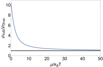
Figure 12: Ratio of the Dirac and holographic charge densities $\rho_{\rm AdS}/\rho_{\rm Dirac}$ as a function of $\mu/k_{B}T$. The black dashed line denotes $\rho_{\rm AdS}/\rho_{\rm Dirac}=1$.

For $g=2$, the phenomenological approach described yields $N\simeq 24$. We can therefore state that the approach we chose here of matching charge densities is self-consistent as it leads to a large value of $N\gg 1$, which is large enough to also suppress quantum gravitational $1/N^{2}$ corrections. We will use this value of $N$ for numerical estimates. Figure 12 shows the ratio between the charge densities from the Fermi-Dirac distribution and from holography. The difference is small for $\mu/k_{B}T>10$, and not too large for values closer to the charge neutrality point. This is due to the coinciding $\mu/k_{B}T$ dependence of both densities for $\mu>k_{B}T$. The dependence on $\mu/(k_{B}T)$ also drops out in this ratio for $\mu/(k_{B}T)\ll 1$. We hence could have matched the two distributions at the charge neutrality point as well, obtaining a slightly smaller value of $N\simeq 5$.

Phenomenological extrapolations from strongly coupled models have been widely employed in QCD.Hoyos et al. (2016); Casalderrey-Solana et al. (2014) Experience with these models of QCD tells that $N=3$ is already large enough to make quantitative statements at the $10\%$ level,Casalderrey-Solana et al. (2014) even at ’t Hooft coupling constants that are not far from $1$.

Finally, we comment on the quantum critical conductivity (IV.12) from AdS/CFT models such as (A.1). One reason for the naturalness of $\sigma_{Q}=e^{2}/h$ is the electromagnetic self-duality of the holographic action (A.1) if the Maxwell term is normalized canonically to $-\frac{1}{4}F_{\mu\nu}^{2}$.Herzog et al. (2007) This emergent discrete symmetry fixes $\sigma_{Q}=e^{2}/h$ in the Dirac regime $\mu/(k_{B}T)\ll 1$. Finite coupling corrections which break the self-duality can be calculated from universal higher derivative terms on the gravity side of the AdS/CFT correspondence.Myers et al. (2011) In summary, there is ample evidence that $\sigma_{Q}=e^{2}/h$ is the strong coupling limit of the perturbative quantum critical conductance $\sigma_{Q}=e^{2}/h$, which motivates our choice of normalization of the $F^{2}$ term in (A.1).

Appendix B Reynolds number for relativistic hydrodynamics

In the present appendix we derive the Reynolds number, $Re$, for relativistic flows. In non-relativistic hydrodynamics, $Re$ appears in the dimensionless Navier-Stokes equations as

$${D\vec{v}\over Dt}=-\nabla P+{1\over Re_{NS}}\triangledown^{2}\vec{v}$$ (B.1)

where ${D\over Dt}\equiv\partial_{t}+\vec{v}\cdot\nabla$ is the convective derivative.

A similar definition for $Re$ does not exist for relativistic hydrodynamics; we amend this below.

Our first derivation of $Re$ mimics the derivation of $Re_{NS}$; we’ll bring the relativistic equations of motion (EOM), $\partial_{\mu}T^{\mu\nu}=0$, into a form similar to the Navier-Stokes equations, and read off $Re$. Thus, we have

$$\begin{split}{1\over v^{2}_{F}}{D\vec{u}\over D\tau}&=-\left({\vec{u}\over v^{2}_{F}}{D\over D\tau}+\nabla\right)\ln(\varepsilon+p)-{\eta\over\varepsilon+p}\vec{\Sigma}\\ &\vec{\Sigma}^{i}\equiv\partial_{\mu}\sigma^{\mu i}\;,\;i=1,2\;,\;{D\over D\tau}\equiv u^{\mu}\partial_{\mu}\end{split}$$ (B.2)

Equation (B.2) is clearly the relativistic counterpart of the Navier-Stokes equations, (B.1). We bring (B.2) into a dimensionless form by applying the transformation $\vec{u}\rightarrow{\vec{u}/v_{\rm max}}\;,\;x^{\mu}\rightarrow{x^{\mu}/W}$, where $v_{\rm max}\equiv|\vec{u}|(y=W/2),W$ are the characteristic velocity and length scales of our flows (see Figure 1.). The result is

$${D\vec{u}\over D\tau} =-\left[\vec{u}{D\over D\tau}+\left({v_{F}\over v_{\rm max}}\right)^{2}\nabla\right]\ln(\varepsilon+p)$$

$$-\left({v_{F}\over v_{\rm max}}\right)^{2}{\eta v_{\rm max}\over W(\varepsilon+p)}\vec{\tilde{\Sigma}},$$ (B.3)

where $\vec{\tilde{\Sigma}}$ is the rescaled version of $\vec{\Sigma}$.

Now we can use (B) in order to read off $Re$. Unfortunately, there is not a single dimensionless number multiplying the second term in the r.h.s. of (B), because of $\vec{\tilde{\Sigma}}$. Thus there is no natural definition of $Re$ in the relativistic case. We can bypass this problem by considering the non-relativistic (NR) and the ultra-relativistic (UR) limits of (B).

• non-relativistic limit: In this case, $v_{F}/v_{\rm max}\gg 1$, and the non-relativistic $Re$ is

  $$Re_{NR}={(\varepsilon+p)W\over\eta v_{\rm max}}\left({v_{\rm max}\over v_{F}}\right)^{2}.$$ (B.4)

  $Re_{NR}$ is proportional to the Navier-Stokes $Re$. We see this if we substitute $\varepsilon=\rho v^{2}_{F}$ and $p={1\over 2}\epsilon$ , where $\rho$ is the fluid mass density, into (B.4) i.e.

  $$Re_{NR}={3\over 2}Re_{NS}={3\over 2}{\rho v_{\rm max}W\over\eta}.$$ (B.5)

• ultra-relativistic limit: In this case, we keep the terms proportional to $({v_{\rm max}/v_{F}})^{4}$ in $\vec{\tilde{\Sigma}}$ and obtain

  $$Re_{UR}={(\varepsilon+p)W\over\eta v_{\rm max}}\left({v_{F}\over v_{\rm max}}\right)^{2}.$$ (B.6)

Our second derivation of $Re$ is based on the physical meaning of $Re$, which is defined as the ratio of inertial forces to the ratio of viscous forces. As usual, the inertial and viscous forces are given by

$$F^{i}_{in}=\partial_{t}T^{0i}\;,\;F^{i}_{v}=-\eta\partial_{j}\sigma^{ji}\;,\;i=1,2$$ (B.7)

Therefore $Re$ can be defined through the ratio $\vec{F}_{in}/\vec{F}_{v}$. Computing this ratio leads us, as expected, to equations (B.5) and (B.6).

Equations (B.5) and (B.6) above summarize our derivation of $Re$ for non-relativistic and ultra-relativistic fluids.

References

- Narozhny et al. (2017) B. N. Narozhny, I. V. Gornyi, A. D. Mirlin, and J. Schmalian, (2017), 1704.03494 .
- Lucas and Fong (2017) A. Lucas and K. C. Fong, (2017), 1710.08425 .
- Molenkamp and de Jong (1994a) L. W. Molenkamp and M. J. M. de Jong, Solid-State Electronics 37, 551 (1994a).
- Molenkamp and de Jong (1994b) L. W. Molenkamp and M. J. M. de Jong, Physical Review B 49, 5038 (1994b).
- de Jong and Molenkamp (1995) M. J. M. de Jong and L. W. Molenkamp, Physical Review B 51, 13389 (1995), cond-mat/9411067 .
- Crossno et al. (2015) J. Crossno, J. K. Shi, K. Wang, X. Liu, A. Harzheim, A. Lucas, S. Sachdev, P. Kim, T. Taniguchi, K. Watanabe, T. A. Ohki, and K. C. Fong, Science , 1058 (2015), 1509.04713 .
- Moll et al. (2016) P. J. W. Moll, P. Kushwaha, N. Nandi, B. Schmidt, and A. P. Mackenzie, Science 351, 1061 (2016), arXiv:1509.05691 [cond-mat.str-el] .
- Bandurin et al. (2016) D. Bandurin, I. Torre, R. K. Kumar, M. B. Shalom, A. Tomadin, A. Principi, G. Auton, E. Khestanova, K. Novoselov, I. Grigorieva, et al., Science 351, 1055 (2016).
- Nam et al. (2017) Y. Nam, D.-K. Ki, D. Soler-Delgado, and A. F. Morpurgo, Nature Physics 13, 1207 (2017).
- Gurzhi (1968) R. N. Gurzhi, Soviet Physics Uspekhi 11, 255 (1968).
- Note (1) In order to meaningfully extract the hydrodynamic shear viscosity, the conditions for hydrodynamics need to apply as a low-energy effective theory. These conditions are e.g. spelled out in sec. II.1. Otherwise the result for the viscosity from e.g. the Kubo formula for the viscosity in quantum field theory or from effective approaches such as kinetic theory will not have a meaningful hydrodynamic interpretation as the viscosity of a fluid in local thermal equilibrium.
- Levitov and Falkovich (2016) L. Levitov and G. Falkovich, Nature Physics 12, 672 (2016).
- Pellegrino et al. (2016) F. M. Pellegrino, I. Torre, A. K. Geim, and M. Polini, Physical Review B 94, 155414 (2016).
- Torre et al. (2015) I. Torre, A. Tomadin, A. K. Geim, and M. Polini, Physical Review B 92, 165433 (2015), arXiv:1508.00363 [cond-mat.mes-hall] .
- Tomadin et al. (2014) A. Tomadin, G. Vignale, and M. Polini, Physical Review Letters 113, 235901 (2014).
- Moessner et al. (2018) R. Moessner, P. Surówka, and P. Witkowski, Phys. Rev. B 97, 161112 (2018).
- Kashuba et al. (2018) O. Kashuba, B. Trauzettel, and L. W. Molenkamp, Physical Review B 97, 205129 (2018).
- Maldacena (1998) J. M. Maldacena, Adv. Theor. Math. Phys. 2, 231 (1998), arxiv:9711200 [hep-th] .
- Gubser et al. (1998) S. S. Gubser, I. R. Klebanov, and A. M. Polyakov, Phys.Lett. B428, 105 (1998), arXiv:hep-th/9802109 [hep-th] .
- Witten (1998) E. Witten, Adv.Theor.Math.Phys. 2, 253 (1998), arXiv:hep-th/9802150 [hep-th] .
- Casalderrey-Solana et al. (2014) J. Casalderrey-Solana, H. Liu, D. Mateos, K. Rajagopal, and U. A. Wiedemann, Gauge/string duality, hot QCD and heavy ion collisions (Cambridge University Press, 2014).
- Ammon and Erdmenger (2015) M. Ammon and J. Erdmenger, Gauge/Gravity Duality: Foundations and Applications (Cambridge University Press, 2015).
- Zaanen et al. (2015) J. Zaanen, Y. Liu, Y.-W. Sun, and K. Schalm, Holographic duality in condensed matter physics (Cambridge University Press, 2015).
- Hartnoll et al. (2016) S. A. Hartnoll, A. Lucas, and S. Sachdev, (2016), arXiv:1612.07324 [hep-th] .
- Note (2) There are examples where hidden conserved quantities together with a long-range disorder potential invalidate the hydrodynamic approximation Lucas and Hartnoll (2018).
- Zaanen (2004) J. Zaanen, Nature 430, 512 (2004).
- Note (3) For an explanation of this fact, c.f. e.g. sec. 3.5 of Hartnoll et al. (2016).
- Bhattacharyya et al. (2008a) S. Bhattacharyya, V. E. Hubeny, S. Minwalla, and M. Rangamani, JHEP 02, 045 (2008a), arXiv:0712.2456 [hep-th] .
- Bhattacharyya et al. (2008b) S. Bhattacharyya, V. E. Hubeny, R. Loganayagam, G. Mandal, S. Minwalla, T. Morita, M. Rangamani, and H. S. Reall, JHEP 06, 055 (2008b), arXiv:0803.2526 [hep-th] .
- Bhattacharyya et al. (2009) S. Bhattacharyya, R. Loganayagam, S. Minwalla, S. Nampuri, S. P. Trivedi, and S. R. Wadia, JHEP 02, 018 (2009), arXiv:0806.0006 [hep-th] .
- Blake (2015) M. Blake, JHEP 09, 010 (2015), arXiv:1505.06992 [hep-th] .
- Policastro et al. (2001) G. Policastro, D. T. Son, and A. O. Starinets, Phys. Rev. Lett. 87, 081601 (2001), arXiv:hep-th/0104066 [hep-th] .
- Kovtun et al. (2005) P. Kovtun, D. T. Son, and A. O. Starinets, Phys. Rev. Lett. 94, 111601 (2005), arXiv:hep-th/0405231 [hep-th] .
- Note (4) For rotationally non-invariant systems, there can be violations of the bound, Mateos and Trancanelli (2011a); Rebhan and Steineder (2012). However, all such violations that have been found so far to leading order in the inverse string tension (dual to the coupling constant) or the gauge group rank (controlling the large limit) occur in unstable ground state, Mateos and Trancanelli (2011a, b). On the other hand, in systems with rotationally non-invariant but obviously stable ground states, the KSS bound (I.3) seems to be observed for all components of the viscosity tensor Erdmenger et al. (2013). To subleading order in (corresponding to finite coupling corrections), violations of (I.3) induce causality violations in the dual field theory Brigante et al. (2008); Camanho et al. (2016). Presumably only string theories including all order corrections is causal Camanho et al. (2016), but has never bee calculated in such a setup. Similar remarks apply to finite corrections Kats and Petrov (2009) which also correspond to higher derivative terms in the dual gravitational theory. In summary, there is good evidenceCremonini (2011) that (I.2\@@italiccorr) holds in the stable ground states of all consistent models.
- Delacrétaz et al. (2018) L. V. Delacrétaz, T. Hartman, S. A. Hartnoll, and A. Lewkowycz, (2018), arXiv:1805.04194 [hep-th] .
- Hartman et al. (2017) T. Hartman, S. A. Hartnoll, and R. Mahajan, Phys. Rev. Lett. 119, 141601 (2017), arXiv:1706.00019 [hep-th] .
- Song et al. (2011) H. Song, S. A. Bass, U. Heinz, T. Hirano, and C. Shen, Physical Review Letters 106, 192301 (2011).
- Note (5) For electrons in solids we have direct access to the hydrodynamic regime. In QCD, we need to reconstruct the hydrodynamic regime from the data collected by particle detectors back through the hadronization crossover.
- Novoselov et al. (2005) K. S. Novoselov, A. K. Geim, S. Morozov, D. Jiang, M. Katsnelson, I. Grigorieva, S. Dubonos, Firsov, and AA, nature 438, 197 (2005).
- König et al. (2007) M. König, S. Wiedmann, C. Brüne, A. Roth, H. Buhmann, L. W. Molenkamp, X.-L. Qi, and S.-C. Zhang, Science 318, 766 (2007).
- Klinkhamer and Volovik (2005) F. R. Klinkhamer and G. E. Volovik, Int. J. Mod. Phys. A20, 2795 (2005), arXiv:hep-th/0403037 [hep-th] .
- Volovik (2006) G. E. Volovik, Int. Ser. Monogr. Phys. 117, 1 (2006).
- Wan et al. (2011) X. Wan, A. M. Turner, A. Vishwanath, and S. Y. Savrasov, Phys. Rev. B 83, 205101 (2011).
- Fritz et al. (2008) L. Fritz, J. Schmalian, M. Müller, and S. Sachdev, Physical Review B 78, 085416 (2008), arXiv:0802.4289 .
- Müller et al. (2009) M. Müller, J. Schmalian, and L. Fritz, Physical Review Letters 103, 025301 (2009), arXiv:0903.4178 [cond-mat.mes-hall] .
- Note (6) In experiment, the channels are typically prepared by etching them out of a thin layer of material. During that process, the channel edges are sufficiently disordered, such that zero velocity boundary conditions are applicable.
- Note (7) In this work, we assume that we can vary independently of . This amounts to varying the coupling strength independent of the temperature, in which case, the entropy density at fixed temperature is a constant in thermal and chemical equilibrium. We leave the investigation on the possible experimental realization for the future.
- Note (8) The appearance of new non-hydrodynamic modes at finite couplingGrozdanov et al. (2016) may invalidate the hydrodynamic approximation. However, we note that in the present work our analysis is performed at finite density in 2+1 dimensions, while these resultsGrozdanov et al. (2016) apply to 3+1 dimensions at vanishing density. Since the structure of higher derivative terms in 3+1 dimensional gravity will be very different from the ones in 4+1 dimensional gravity, these resultsGrozdanov et al. (2016) are not directly applicable to our analysis. We note that in the context of applying AdS/CFT to heavy ion physics, the physical implications of these terms are still under debate.Strickland (2018) At present we therefore consider our monotonic coupling interpolation to be in the hydrodynamic regime. We point out that a detailed analysis of this issue will be necessary in 2+1 dimensions and at finite density as well.
- Davison et al. (2014) R. A. Davison, K. Schalm, and J. Zaanen, Physical Review B 89, 245116 (2014).
- Landau and Lifshitz (1987) L. Landau and E. Lifshitz, Fluid Mechanics, 2nd ed., Course of Theoretical Physics S (Butterworth-Heinemann, 1987).
- Romatschke (2010) P. Romatschke, International Journal of Modern Physics E 19, 1 (2010).
- Luciano Rezzolla (2013) O. Z. Luciano Rezzolla, Relativistic Hydrodynamics (Oxford University Press, 2013).
- Note (9) Introducing a nontrivial metric is useful when e.g. considering perturbations that correspond to a temperature gradient acting on the fluid Kadanoff and Martin (1963), and can be achieved by replacing partial derivatives in (II.4\@@italiccorr)-(II.5\@@italiccorr) by the covariant derivative with an appropriately chosen connection, which most of the time will be the metric compatible Christoffel connection.
- Note (10) We normalized the electric field by means of the fundamental constants and and in such a way that and .
- Note (11) Another common frame is Eckart frame, in which the fluid is comoving w.r.t. the current flow, amounting to in (II.7b\@@italiccorr). Another example can be found in Jensen et al. (2012), where the in the presence of a constant magnetic field can either be considered zeroth order in derivatives due to the constancy of and incorporated into the pressure, or, if is small, to be of first order due to the fact that the magnetic field is the derivative of the vector potential. It is possible to switch between both frames through field transformations, Kovtun (2012).
- Note (12) Scale invariance implies vanishing stress-energy tensor trace, =0, and hence . Furthermore, due to renormalization effects the Fermi velocity runs logarithmically at low temperatures Lucas and Fong (2017). Another reason for neglecting the bulk viscosity term is that we are working with incompressible fluid flows, i.e. .
- Note (13) The conservation equation for the current (II.5\@@italiccorr) is trivially satisfied for the flow we will introduce in sec. III, and hence we do not discuss it hereafter.
- Bruin et al. (2013) J. Bruin, H. Sakai, R. Perry, and A. Mackenzie, Science 339, 804 (2013).
- Gooth et al. (2017) J. Gooth, F. Menges, C. Shekhar, V. Süß, N. Kumar, Y. Sun, U. Drechsler, R. Zierold, C. Felser, and B. Gotsmann, arXiv preprint arXiv:1706.05925 (2017).
- Note (14) Note that we assume vanishing temperature gradients. If we were to relax this assumption, the spacetime dependence of should also be taken into account in the equations of motion.
- Vegh (2013) D. Vegh, (2013), arXiv:1301.0537 [hep-th] .
- Andrade and Withers (2014) T. Andrade and B. Withers, Journal of High Energy Physics 2014, 101 (2014).
- Davison (2013) R. A. Davison, Phys. Rev. D88, 086003 (2013), arXiv:1306.5792 [hep-th] .
- Brüne et al. (2014) C. Brüne, C. Thienel, M. Stuiber, J. Böttcher, H. Buhmann, E. G. Novik, C.-X. Liu, E. M. Hankiewicz, and L. W. Molenkamp, Physical Review X 4, 041045 (2014), arXiv:1407.6537 [cond-mat.mes-hall] .
- Majumder et al. (2007) A. Majumder, B. Müller, and X.-N. Wang, Phys. Rev. Lett. 99, 192301 (2007), arXiv:hep-ph/0703082 [hep-ph] .
- Buchel et al. (2005) A. Buchel, J. T. Liu, and A. O. Starinets, Nucl. Phys. B707, 56 (2005), arXiv:hep-th/0406264 [hep-th] .
- Note (15) We recall that is a priori physically independent of the electron-electron scattering rate .
- Hartnoll et al. (2007) S. A. Hartnoll, P. K. Kovtun, M. Müller, and S. Sachdev, Phys. Rev. B76, 144502 (2007), arXiv:0706.3215 [cond-mat.str-el] .
- Hartnoll and Herzog (2007) S. A. Hartnoll and C. P. Herzog, Phys. Rev. D76, 106012 (2007), arXiv:0706.3228 [hep-th] .
- Note (16) The quantum critical resistance is defined via Ohm’s law, , with the cross-sectional area of the wire. Here .
- Note (17) We assume that holds, such that we are in the hydrodynamic regime.
- Hanks (1963) R. W. Hanks, AIChE Journal 9, 45 (1963).
- Hanks (1969) R. W. Hanks, AIChE Journal 15, 25 (1969).
- Mendoza et al. (2011) M. Mendoza, H. J. Herrmann, and S. Succi, Physical Review Letters 106, 156601 (2011), arXiv:1201.6590 [cond-mat.mes-hall] .
- Note (18) We define the kinematic viscosity as the ratio of viscosity and energy density. There exists another kinematic viscosity, , defined as the ratio of viscosity and mass density. The two viscosities are related by .
- Note (19) A measurement of is more readily performed in a bulk sample where viscous effects are negligible, by comparing samples of different impurity content and extrapolating to the clean limit.
- Kiselev and Schmalian (2018) E. I. Kiselev and J. Schmalian, arXiv.org (2018), 1806.03933v2 .
- Goutéraux (2014) B. Goutéraux, JHEP 04, 181 (2014), arXiv:1401.5436 [hep-th] .
- Karch and O’Bannon (2007) A. Karch and A. O’Bannon, JHEP 09, 024 (2007), arXiv:0705.3870 [hep-th] .
- Note (20) In particular in the Dirac limit , , and the dependence on thermodynamic variables drops out of (IV.12\@@italiccorr).
- Note (21) In fact, the center flow can be understood as an effective channel flow with no-stress boundary conditions. These conditions are imposed at the edge of a layer of width . These boundary conditions then lead to Ohmic hydrodynamic flow at the center of the channel Lucas and Fong (2017).
- Anninos and Pastras (2009) D. Anninos and G. Pastras, Journal of High Energy Physics 2009, 030 (2009), arXiv:0807.3478 [hep-th] .
- Witczak-Krempa and Sachdev (2012) W. Witczak-Krempa and S. Sachdev, Phys. Rev. B 86, 235115 (2012).
- Witczak-Krempa and Sachdev (2013) W. Witczak-Krempa and S. Sachdev, Phys. Rev. B 87, 155149 (2013).
- Grozdanov and Starinets (2017) S. Grozdanov and A. O. Starinets, Journal of High Energy Physics 2017, 166 (2017).
- Gross and Sloan (1987) D. J. Gross and J. H. Sloan, Nuclear Physics B 291, 41 (1987).
- Jensen et al. (2012) K. Jensen, M. Kaminski, P. Kovtun, R. Meyer, A. Ritz, and A. Yarom, JHEP 05, 102 (2012), arXiv:1112.4498 [hep-th] .
- Hoyos (2014) C. Hoyos, Int. J. Mod. Phys. B28, 1430007 (2014), arXiv:1403.4739 [cond-mat.mes-hall] .
- Pellegrino et al. (2017) F. M. D. Pellegrino, I. Torre, and M. Polini, Physical Review B 96, 195401 (2017), arXiv:1706.08363 [cond-mat.mes-hall] .
- Delacretaz and Gromov (2017) L. V. Delacretaz and A. Gromov, Phys. Rev. Lett. 119, 226602 (2017), [Addendum: Phys. Rev. Lett.120,no.7,079901(2018)], arXiv:1706.03773 [cond-mat.str-el] .
- Note (22) A black brane is a black hole with planar horizon topology, in this case .
- de Haro et al. (2001) S. de Haro, S. N. Solodukhin, and K. Skenderis, Commun. Math. Phys. 217, 595 (2001), arXiv:hep-th/0002230 [hep-th] .
- Papadimitriou and Skenderis (2004) I. Papadimitriou and K. Skenderis, JHEP 10, 075 (2004), arXiv:hep-th/0407071 [hep-th] .
- Papadimitriou and Skenderis (2005) I. Papadimitriou and K. Skenderis, JHEP 08, 004 (2005), arXiv:hep-th/0505190 [hep-th] .
- Erdmenger et al. (2017) J. Erdmenger, D. Fernandez, P. Goulart, and P. Witkowski, JHEP 03, 147 (2017), arXiv:1611.09381 [hep-th] .
- Note (23) The renormalization of the Fermi velocity is negligible at most temperatures except exponentially small ones Lucas and Fong (2017).
- Note (24) We in particular do not claim that Einstein-Maxwell holography (A.1) can describe a weakly interacting Fermi liquid regime such as the one present in e.g. graphene at .
- Balasubramanian and McGreevy (2008) K. Balasubramanian and J. McGreevy, Phys. Rev. Lett. 101, 061601 (2008), arXiv:0804.4053 [hep-th] .
- Charmousis et al. (2010) C. Charmousis, B. Gouteraux, B. S. Kim, E. Kiritsis, and R. Meyer, JHEP 11, 151 (2010), arXiv:1005.4690 [hep-th] .
- Aharony et al. (2008) O. Aharony, O. Bergman, D. L. Jafferis, and J. Maldacena, JHEP 10, 091 (2008), arXiv:0806.1218 [hep-th] .
- Hoyos et al. (2016) C. Hoyos, D. Rodríguez Fernández, N. Jokela, and A. Vuorinen, Phys. Rev. Lett. 117, 032501 (2016), arXiv:1603.02943 [hep-ph] .
- Herzog et al. (2007) C. P. Herzog, P. Kovtun, S. Sachdev, and D. T. Son, Phys. Rev. D75, 085020 (2007), arXiv:hep-th/0701036 [hep-th] .
- Myers et al. (2011) R. C. Myers, S. Sachdev, and A. Singh, Phys. Rev. D83, 066017 (2011), arXiv:1010.0443 [hep-th] .
- Note (25) For example, where is the fluid and characteristic velocity, respectively.
- Note (26) Without loss of generality, we have set the external fields to zero and taken .
- Note (27) after rescaling contains terms proportional to .
- Note (28) Recall that the fluid in particular is conformal. This is in contrast to common non-relativistic fluids, for which . In this case, .
- Lucas and Hartnoll (2018) A. Lucas and S. A. Hartnoll, Phys. Rev. B97, 045105 (2018), arXiv:1706.04621 [cond-mat.str-el] .
- Mateos and Trancanelli (2011a) D. Mateos and D. Trancanelli, Phys. Rev. Lett. 107, 101601 (2011a), arXiv:1105.3472 [hep-th] .
- Rebhan and Steineder (2012) A. Rebhan and D. Steineder, Phys. Rev. Lett. 108, 021601 (2012), arXiv:1110.6825 [hep-th] .
- Mateos and Trancanelli (2011b) D. Mateos and D. Trancanelli, JHEP 07, 054 (2011b), arXiv:1106.1637 [hep-th] .
- Erdmenger et al. (2013) J. Erdmenger, D. Fernandez, and H. Zeller, JHEP 04, 049 (2013), arXiv:1212.4838 [hep-th] .
- Brigante et al. (2008) M. Brigante, H. Liu, R. C. Myers, S. Shenker, and S. Yaida, Phys. Rev. Lett. 100, 191601 (2008), arXiv:0802.3318 [hep-th] .
- Camanho et al. (2016) X. O. Camanho, J. D. Edelstein, J. Maldacena, and A. Zhiboedov, JHEP 02, 020 (2016), arXiv:1407.5597 [hep-th] .
- Kats and Petrov (2009) Y. Kats and P. Petrov, JHEP 01, 044 (2009), arXiv:0712.0743 [hep-th] .
- Cremonini (2011) S. Cremonini, Mod. Phys. Lett. B25, 1867 (2011), arXiv:1108.0677 [hep-th] .
- Grozdanov et al. (2016) S. Grozdanov, N. Kaplis, and A. O. Starinets, Journal of High Energy Physics 2016, 151 (2016).
- Strickland (2018) M. Strickland, in 27th International Conference on Ultrarelativistic Nucleus-Nucleus Collisions (Quark Matter 2018) Venice, Italy, May 14-19, 2018 (2018) arXiv:1807.07191 [nucl-th] .
- Kadanoff and Martin (1963) L. P. Kadanoff and P. C. Martin, Annals of Physics 24, 419 (1963).
- Kovtun (2012) P. Kovtun, INT Summer School on Applications of String Theory Seattle, Washington, USA, July 18-29, 2011, J. Phys. A45, 473001 (2012), arXiv:1205.5040 [hep-th] .