A functional approach to estimation of the parameters of generalized negative binomial and gamma distributions

Abstract

The generalized negative binomial distribution (GNB) is a new flexible family of discrete distributions that are mixed Poisson laws with the mixing generalized gamma (GG) distributions. This family of discrete distributions is very wide and embraces Poisson distributions, negative binomial distributions, Sichel distributions, Weibull–Poisson distributions and many other types of distributions supplying descriptive statistics with many flexible models. These distributions seem to be very promising for the statistical description of many real phenomena. GG distributions are widely applied in signal and image processing and other practical problems. The statistical estimation of the parameters of GNB and GG distributions is quite complicated. To find estimates, the methods of moments or maximum likelihood can be used as well as two-stage grid EM-algorithms. The paper presents a methodology based on the search for the best distribution using the minimization of $\ell^{p}$-distances and $L^{p}$-metrics for GNB and GG distributions, respectively. This approach, first, allows to obtain parameter estimates without using grid methods and solving systems of nonlinear equations and, second, yields not point estimates as the methods of moments or maximum likelihood do, but the estimate for the density function. In other words, within this approach the set of decisions is not a Euclidean space, but a functional space.

1 Introduction

The generalized negative binomial distribution (GNB) is a new flexible family of discrete distributions that are mixed Poisson laws with the mixing generalized gamma (GG) distributions. The GNB distributions were introduced and studied in [1] under the name of GG mixed Poisson distributions. This family of discrete distributions is very wide and embraces Poisson distributions (as limit points corresponding to a degenerate mixing distribution), negative binomial (Polya) distributions including geometric distributions (corresponding to the gamma mixing distribution, see [2]), Sichel distributions (corresponding to the inverse gamma mixing distributions, see [3]), Weibull–Poisson distributions (corresponding to the Weibull mixing distributions, see [4]) and many other types supplying descriptive statistics with many flexible models. These distributions seem to be very promising for the statistical description of many real phenomena being very convenient and almost universal models. It is quite natural to expect that, having introduced one more free parameter into the pure negative binomial model, namely, the power parameter in the exponent of the original gamma mixing distribution, instead of the negative binomial model one might obtain a more flexible GNB model that provides even better fit with the statistical data. For example, GNB distributions can be successfully applied to modeling statistical regularities in duration of specific periods in data.

The GG distributions are proposed in order to have a flexible Bayesian model with a mixing (prior) distribution which is “responsible” for the description of statistical regularities of the manifestation of external stochastic factors. The class of GG distributions was first described as a unitary family in $1962$ by E. Stacy [5]. The family of GG distributions contains practically all the most popular absolutely continuous distributions concentrated on the non-negative half-line including Weibull and gamma distributions.

GG distributions are widely applied in many practical problems. There are dozens of papers dealing with the application of GG distributions as models of regularities observed in practice. As an example, the following research areas involving models based on GG distributions can be mentioned:

• climatic and hydrological problems: drop size distributions [6], drought data [7], phenomena in warm clouds [8];

• synthetic-aperture radar (SAR) image processing and various applications: distribution for the real and imaginary parts of the complex SAR backscattered signal [9], flexible model for the SAR images with different land-cover typologies [10], statistical modeling of SAR images [11, 12];

• astrophysical problems, for example, new galaxy luminosity functions [13];

• speech signal processing: parametric characterization of speech spectra [14], modelling speech samples [15], real-time implementations of algorithms [16].

Apparently, the popularity of GG distributions is due to that most of them can serve as adequate asymptotic approximations, since all the representatives of the class of GG distributions listed above appear as limit laws in various limit theorems of probability theory in rather simple limit schemes.

The problem of statistical estimation of the parameters of GNB and GG distributions (for example, the search for maximum likelihood (ML) estimates) is quite complicated. To find the estimates of the parameters, the method of moments or ML method [17] for the GG distribution as well as the two-stage grid EM-algorithm for the GNB, can be used. It should be noted that the implementations of the methods of moments and ML method for GG distribution are difficult computational tasks, moreover, the efficiency depends on the sample size (ML method is better for large volumes).

The paper presents a methodology based on finding the best distribution using minimization of $\ell^{1}$-, $\ell^{2}$- and $\ell^{\infty}$-distances and $L^{1}$-, $L^{2}$- and $L^{\infty}$-metrics for GNB and GG distributions, respectively. This approach, first, allows to obtain parameter estimates without using grid methods and solving systems of nonlinear equations and, second, yields not point estimates as the methods of moments or maximum likelihood do, but the estimate for the density function. In other words, within this approach the set of decisions is not a Euclidean space, but a functional space.

2 The GNB and GG distributions

It will be assumed that all the random variables are defined on the same probability space $(\Omega,\,\mathfrak{F},\,{\mathbb{P}})$.

A random variable having the gamma distribution with shape parameter $r>0$ and scale parameter $\mu>0$ will be denoted $G_{r,\mu}$,

$$\mathbb{P}(G_{r,\mu}<x)=\int_{0}^{x}g(z;r,\mu)dz,\ \ \text{with}\ \ g(x;r,\mu)=\frac{\mu^{r}}{\Gamma(r)}x^{r-1}e^{-\mu x},\ x\geq 0,$$ (1)

where $\Gamma(r)$ is Euler’s gamma-function, $\Gamma(r)=\int_{0}^{\infty}x^{r-1}e^{-x}dx$, $r>0$.

A GG distribution is the absolutely continuous distribution defined by the density

$$g^{*}(x;r,\gamma,\mu)=\frac{|\gamma|\mu^{r}}{\Gamma(r)}x^{\gamma r-1}e^{-\mu x^{\gamma}},\ \ \ \ x\geq 0,$$ (2)

with $\gamma\in\mathbb{R}$, $\mu>0$, $r>0$. The distribution function corresponding to the density $g^{*}(x;r,\gamma,\mu)$ can be denoted $F^{*}(x;r,\gamma,\mu)$.

The properties of GG distributions were described in [5, 18]. A random variable with the density $g^{*}(x;r,\gamma,\mu)$ will be denoted $\overline{G}_{r,\gamma,\mu}$. It can be easily made sure that

$$\overline{G}_{r,\gamma,\mu}\stackrel{{\scriptstyle d}}{{=}}G_{r,\mu}^{1/\gamma},$$ (3)

and hence,

$$(\overline{G}_{r,\gamma,\mu})^{\gamma}\stackrel{{\scriptstyle d}}{{=}}G_{r,\mu}.$$ (4)

The symbol $\stackrel{{\scriptstyle d}}{{=}}$ in (3) and (4) denotes the coincidence of distributions.

A random variable $N_{r,p}$ is said to have the negative binomial (NB) distribution with parameters $r>0$ (“shape”) and $p\in(0,1)$ (“success probability”), if

$${\mathbb{P}}(N_{r,p}=k)=\frac{\Gamma(r+k)}{k!\Gamma(r)}\cdot p^{r}(1-p)^{k},\ \ \ \ k=0,1,2,...$$ (5)

Let $r>0$, $\gamma\in\mathbb{R}$ and $\mu>0$. We say that the random variable $N_{r,\gamma,\mu}$ has the GNB distribution, if

$${\mathbb{P}}(N_{r,\gamma,\mu}=k)=\frac{1}{k!}\int_{0}^{\infty}e^{-z}z^{k}g^{*}(z;r,\gamma,\mu)dz,\ \ \ \ k=0,1,2...,$$ (6)

and $g^{*}(z;r,\gamma,\mu)$ is determined by formula (2).

3 A functional approach to estimation of the parameters of GNB distributions

The problem of statistical estimation of the parameters of GNB distribution (for example, the search for maximum likelihood estimates) is extremely complicated. To find estimators, the two-stage grid EM-algorithm for the GNB distribution $F(x;r,\gamma,\mu)$ can be used. At the first stage, the main part of the support of the mixing distribution is determined. That is, a bounded interval is determined such that the probability of a GG distributed mixing random variable to fall into this interval is insignificantly less than one. This interval is covered by a finite grid containing (possibly, a very large number) $K\in\mathbb{N}$ of known nodes $\lambda_{1},...,\lambda_{K}$. The GNB distribution under study is approximated by the finite mixture of Poisson distributions:

$$F(x;r,\gamma,\mu)(x+0)\approx\sum_{j=0}^{[x]}\frac{1}{j!}\sum_{i=1}^{K}p_{i}e^{-\lambda_{i}}\lambda_{i}^{j},\ \ \ x\in\mathbb{R}.$$ (7)

In the mixture on the right-hand side of (7), only the parameters $p_{1},...,p_{K}$ are unknown. At the second stage, it remains to use some standard method for fitting the GG distribution to the histogram-type data $(\mu_{1},p_{1}),...,(\mu_{K},p_{K})$, obtained at the first stage. For example, the parameters $r$, $\gamma$ and $\mu$ can be determined as the point minimizing the corresponding chi-square statistic or some special least squares problem.

However, with a fixed grid, the two-stage method yields only approximate estimates of the parameters of GG distributions. Moreover, the accuracy of the approximation depends on the choice of the grid. The estimates can be consistent in the traditional sense only if the grid mesh becomes infinitely small as the sample size infinitely increases in an appropriate way. Moreover, the conditions unifying the rate of decrease of the grid mesh with the rate of increase of the sample size that provide the statistical consistency of the estimators are very cumbersome and practically unverifiable.

In this section we present an alternative methodology based on finding the best GNB distribution using minimization of $\ell^{1}$-, $\ell^{2}$- and $\ell^{\infty}$-distances (they correspond to the spaces of sequences whose series are absolutely convergent, the space of square-summable sequences and the space of bounded sequences, respectively). Namely, the histogram of the initial data should be obtained. The integer rule is used as bining algorithm (due to that the observations in the sample are integer), so bins are created for each value. Let $N_{b}$ be the number of histogram bins (with a uniform width that equals $1$), $\bf h$ be the vector of bar heights ($h_{i}\in[0,1]$ for all $i=1,\ldots,N_{b}$). The value of each component $h_{i}$ is equal to the ratio of a number of observations in the bin to a total number of observations, the sum of the bar areas is $1$. So, the bars of empirical distribution can be approximated by ones of GNB. For finding estimations of unknown parameters of generalized negative binomial distributions the following optimization problems should be solved (the density $g^{*}(x;r,\gamma,\mu)$ is determined by (2) and the probability ${\mathbb{P}}(N_{r,\gamma,\mu}=k)$ is determined by (6)).

• If the target function is based on $\ell^{1}$-distance:

  $$(r^{*},\gamma^{*},\mu^{*})=\arg\min_{r,\gamma,\mu}\sum\limits_{k=1}^{N_{b}}\left|\frac{1}{k!}\int_{0}^{\infty}e^{-z}z^{k}g^{*}(z;r,\gamma,\mu)dz-h_{k}\right|.$$ (8)

• If the target function is based on $\ell^{2}$-distance:

  $$(r^{*},\gamma^{*},\mu^{*})=\arg\min_{r,\gamma,\mu}\sqrt{\sum\limits_{k=1}^{N_{b}}\left(\frac{1}{k!}\int_{0}^{\infty}e^{-z}z^{k}g^{*}(z;r,\gamma,\mu)dz-h_{k}\right)^{2}}.$$ (9)

• If the target function is based on $\ell^{\infty}$-distance:

  $$(r^{*},\gamma^{*},\mu^{*})=\arg\min_{r,\gamma,\mu}\max\limits_{k=\overline{1,N_{b}}}\left|\frac{1}{k!}\int_{0}^{\infty}e^{-z}z^{k}g^{*}(z;r,\gamma,\mu)dz-h_{k}\right|.$$ (10)

Formulas (8)–(10) allow to obtain parameter estimates without using grid methods. It should be noted that this methodology can also be used for the classical negative binomial distribution (5) (the ratio (5) should be used in formulas (8)–(10) instead of (6)).

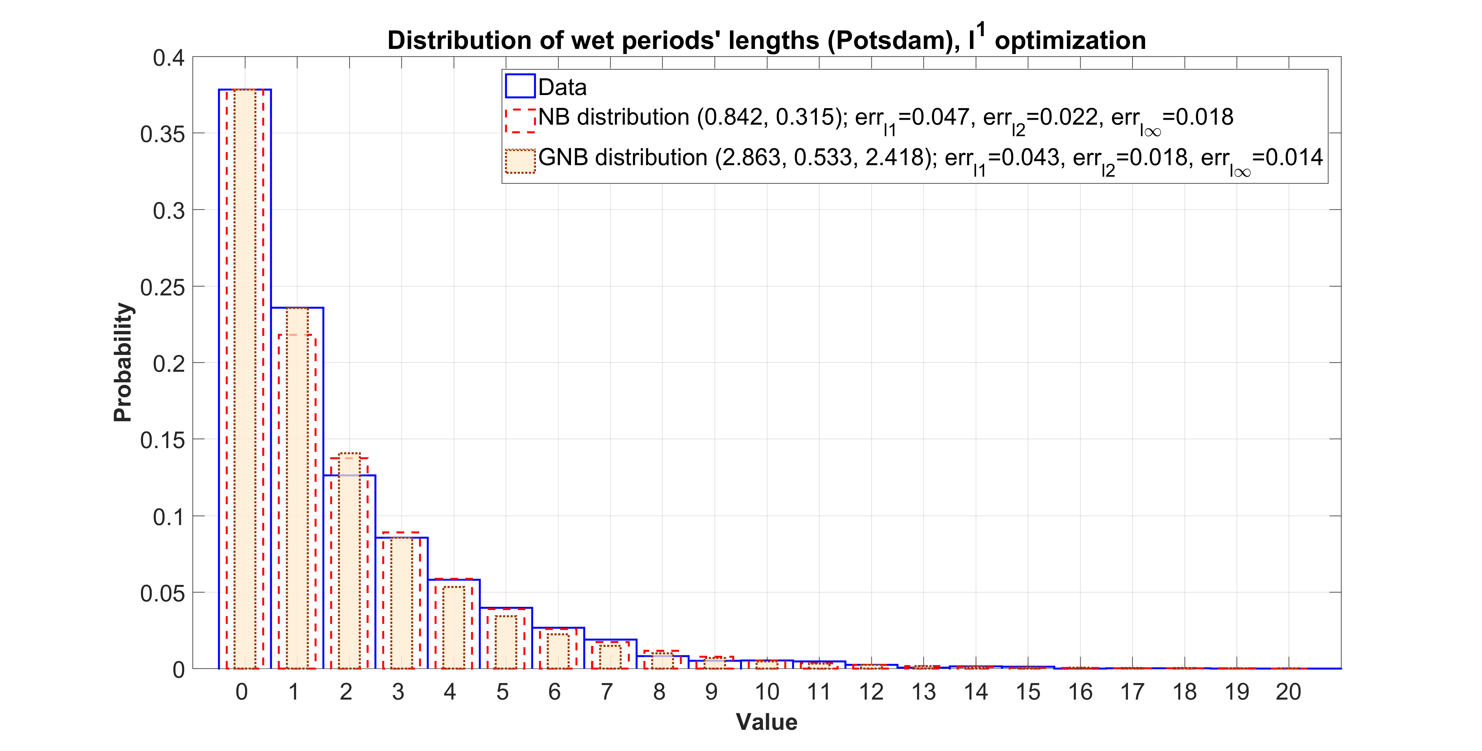
Figure 1: Approximation of the initial data distribution by optimization of $\ell^{1}$-distance.

A special MATLAB program is implemented for finding GNB approximations and plotting figures. The numerical optimization is based on the simplex search method [19]. The functions for estimating the values of all three unknown parameters of the GNB distribution or two parameters provided the shape parameter $r$ estimate based on NB distribution is given are created.

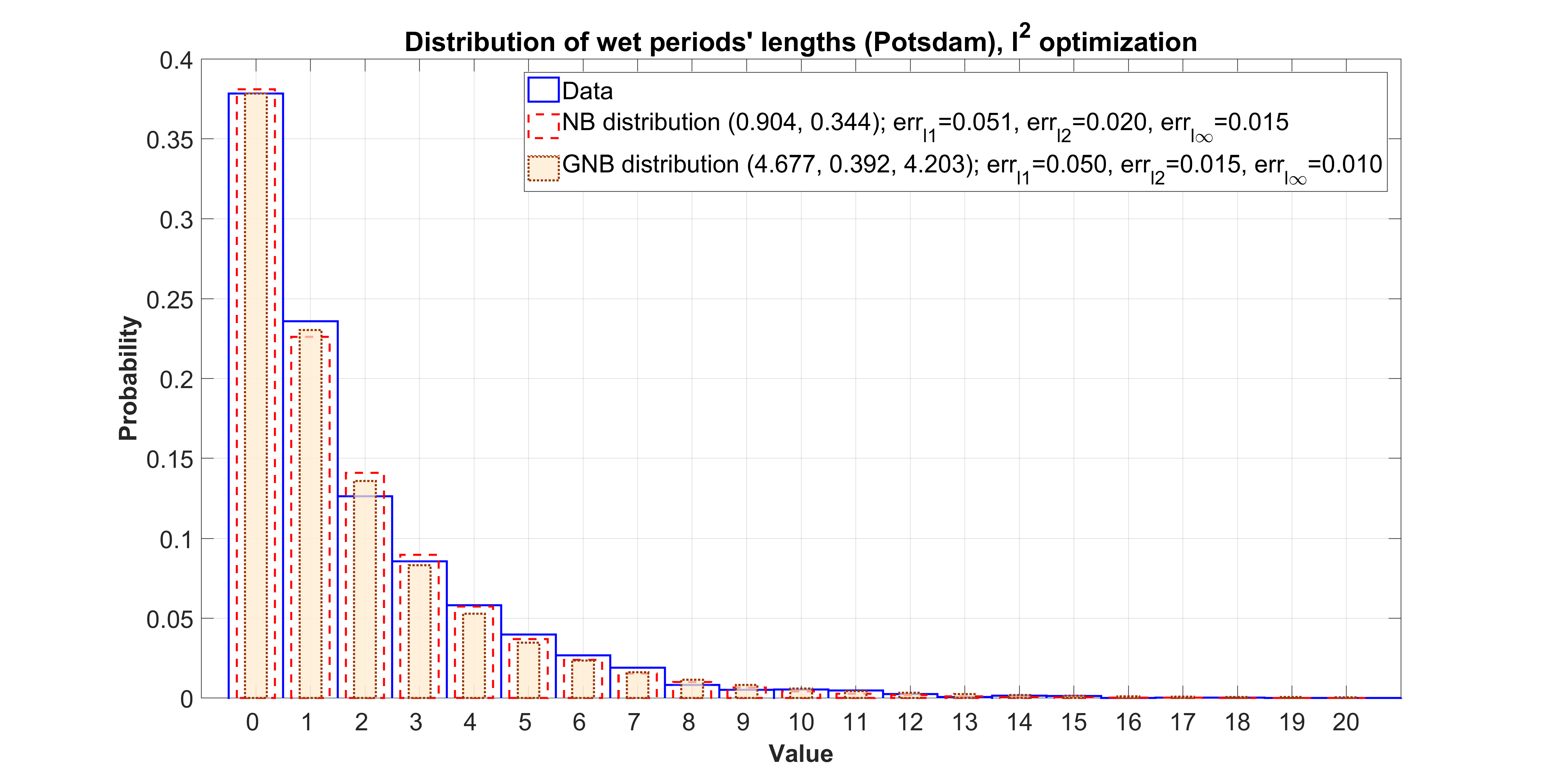
Figure 2: Approximation of the initial data distribution by optimization of $\ell^{2}$-distance.

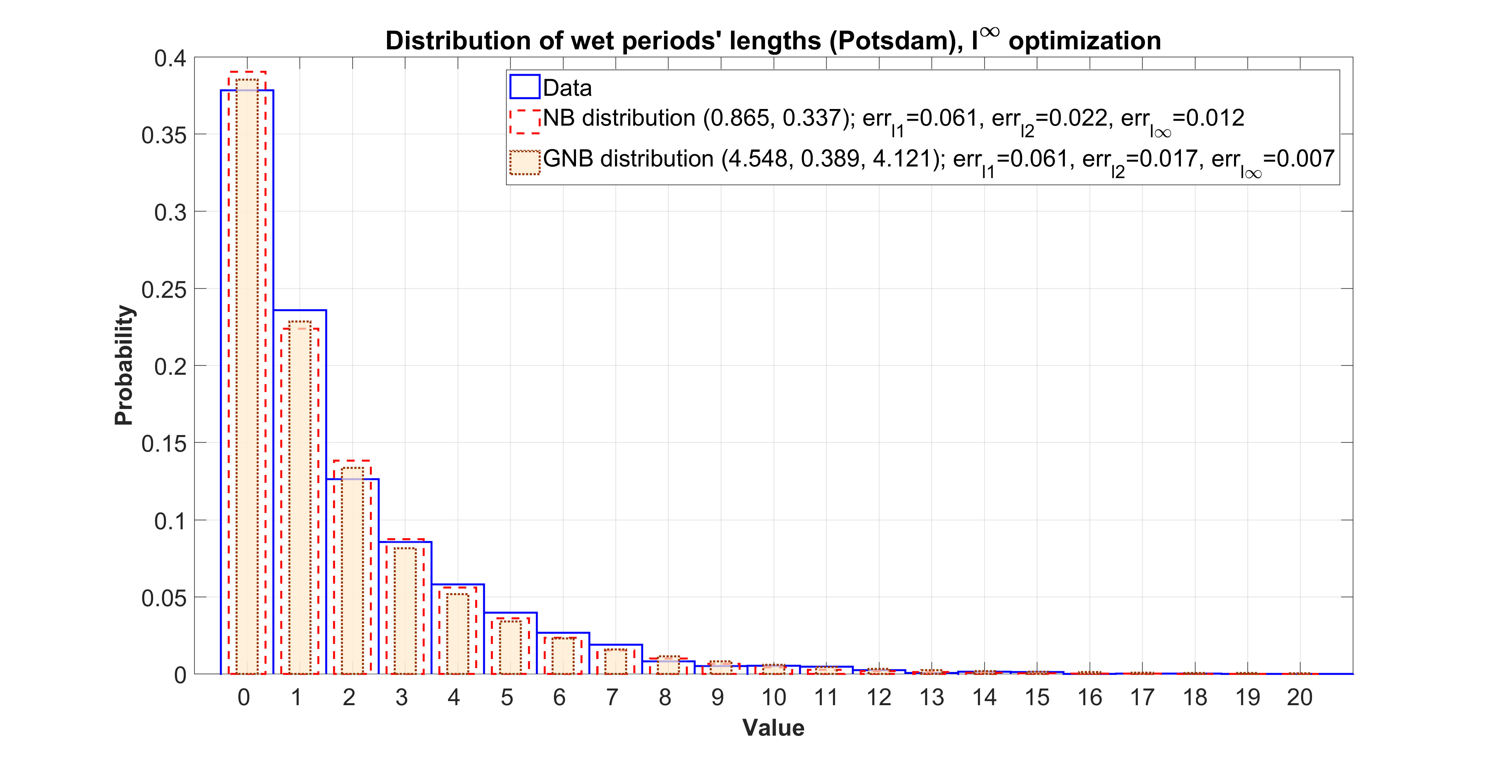
Figure 3: Approximation of the initial data distribution by optimization of $\ell^{\infty}$-distance.

The histogram and approximating graphs of the NB and GNB distributions as well as errors in the corresponding metrics are plotted. The examples of results are shown on Figs. 1–3. They demonstrate a high quality of the approximation of the histogram of the initial data by each type of distributions. Table 1 represents approximation errors, the parameters are estimated by each of the metrics. Obviously, the results for GNB distributions are better (see the bold marked items).

Table 1: Approximation errors for negative binomial and generalized negative binomial distributions, test sample.

Distribution	Error ($\ell^{1}$)	Error ($\ell^{2}$)	Error ($\ell^{\infty}$)
NB ($\ell^{1}$-optimization)	$0{,}047$	$0{,}022$	$0{,}018$
GNB ($\ell^{1}$-optimization)	$\bf 0{,}043$	$0{,}018$	$0{,}014$
NB ($\ell^{2}$-optimization)	$0{,}051$	$0{,}0195$	$0{,}015$
GNB ($\ell^{2}$-optimization)	$0{,}05$	$\bf 0{,}015$	$0{,}0097$
NB ($\ell^{\infty}$-optimization)	$0{,}061$	$0{,}022$	$0{,}012$
GNB ($\ell^{\infty}$-optimization)	$0{,}061$	$0{,}017$	$\bf 0{,}007$

4 Recurrence formulas for GNB distributions

Using formulas (2) and (6) we can obtain the following results:

$$\mathbb{P}(N_{r,\gamma,\mu}=k)=\frac{|\gamma|\mu^{r}}{\Gamma(r)k!}\int\limits_{0}^{\infty}e^{-z-\mu z^{\gamma}}\,z^{\gamma r+k-1}\,dz=\frac{|\gamma|\mu^{r}}{\Gamma(r)k!}\int\limits_{0}^{\infty}e^{-z-\mu z^{\gamma}}\,d\frac{z^{\gamma r+k}}{\gamma r+k}=$$

$$=\frac{|\gamma|\mu^{r}}{\Gamma(r)k!}\times\left[\frac{z^{\gamma r+k}}{\gamma r+k}\,e^{-z-\mu z^{\gamma}}\bigg{|}_{0}^{\infty}-\int\limits_{0}^{\infty}e^{-z-\mu z^{\gamma}}\frac{z^{\gamma r+k}}{\gamma r+k}(-1-\mu\gamma z^{\gamma-1})\,dz\right]=$$

$$=\frac{|\gamma|\mu^{r}}{\Gamma(r)k!}\times\left[\frac{1}{\gamma r+k}\int\limits_{0}^{\infty}e^{-z-\mu z^{\gamma}}z^{\gamma r+k}\,dz+\frac{\mu\gamma}{\gamma r+k}\int\limits_{0}^{\infty}e^{-z-\mu z^{\gamma}}z^{\gamma r+\gamma+k-1}\,dz\right]=$$

$$=\frac{k+1}{\gamma r+k}\,\mathbb{P}(N_{r,\gamma,\mu}=k+1)+\frac{\gamma^{2}\mu^{r+1}}{(\gamma r+k)\Gamma(r)k!}\int\limits_{0}^{\infty}e^{-z-\mu z^{\gamma}}z^{\gamma r+k-1+\gamma}\,dz=$$

$$=\frac{k+1}{\gamma r+k}\,\mathbb{P}(N_{r,\gamma,\mu}=k+1)+\frac{|\gamma|\mu}{\gamma r+k}\mathbb{P}(N_{r+1,\,\gamma,\mu}=k).$$

So, the recurrence formulas for GNB distributions can be represented as follows:

$$(\gamma r+k)\,\mathbb{P}(N_{r,\gamma,\mu}=k)=(k+1)\,\mathbb{P}(N_{r,\gamma,\mu}=k+1)+|\gamma|\mu\,\mathbb{P}(N_{r+1,\,\gamma,\mu}=k),$$

or

$$\mathbb{P}(N_{r,\gamma,\mu}=k+1)=\frac{\gamma r+k}{k+1}\,\mathbb{P}(N_{r,\gamma,\mu}=k)-\frac{|\gamma|\mu}{k+1}\,\mathbb{P}(N_{r+1,\,\gamma,\mu}=k).$$ (11)

Unfortunately, the representation (11) does not significantly simplify the computational process, since in addition to the value $\mathbb{P}(N_{r,\gamma,\mu}=k)$ a value $\mathbb{P}(N_{r+1,\gamma,\mu}=k)$ should be known.

5 A functional approach to the estimation of the parameters of GG distributions

In this section we present a methodology based on the search for the best GG distribution using minimization of $L^{1}$-, $L^{2}$- and $L^{\infty}$-metrics (they correspond to the spaces of functions for which the $p^{th}$ power of the absolute value is Lebesgue integrable, where functions that agree almost everywhere are identified).

The histogram of the initial data should be obtained. The Freedman–Diaconis rule [20] is used as bining algorithm due to its suitableness for data with heavy-tailed distributions. It uses a bin width of

$$2\,\frac{x_{0{.}75}-x_{0{.}25}}{\sqrt[3]{n}},$$ (12)

where $x_{0{.}25}$, $x_{0{.}75}$ are $0{.}25$- and $0{.}75$-quantiles, numerator of fraction (12) represents an interquartile range and $n$ is a sample size.

Let $N_{b}$ be the number of histogram bins, $\bf h$ be the vector of bar heights ($h_{i}\in[0,1]$ for all $i=1,\ldots,N_{b}$). The value of each component $h_{i}$ is equal to the ratio of the number of observations in the bin and the total number of observations, the sum of the bar areas is $1$. Let $\bf b$ be the vector of bin edges. The bars of empirical distribution should be approximated by GG distribution.

To find the estimates of unknown parameters of GG distributions the following optimization problems should be solved (the density $g^{*}(x;r,\gamma,\mu)$ is determined by (2)).

• If the target function is based on $L^{1}$-metric:

  $$(r^{*},\gamma^{*},\mu^{*})=\arg\min_{r,\gamma,\mu}\sum\limits_{k=1}^{N_{b}-1}\int\limits_{b_{k}}^{b_{k+1}}\left|g^{*}(z;r,\gamma,\mu)-h_{k}\right|\,dz.$$ (13)

• If the target function is based on $L^{2}$-metric:

  $$(r^{*},\gamma^{*},\mu^{*})=\arg\min_{r,\gamma,\mu}\sqrt{\sum\limits_{k=1}^{N_{b}-1}\int\limits_{b_{k}}^{b_{k+1}}\left(g^{*}(z;r,\gamma,\mu)-h_{k}\right)^{2}}\,dz.$$ (14)

• If the target function is based on $L^{\infty}$-metric:

  $$(r^{*},\gamma^{*},\mu^{*})=\arg\min_{r,\gamma,\mu}\max\limits_{k\in[1,N_{b}-1]}\int\limits_{b_{k}}^{b_{k+1}}\left|g^{*}(z;r,\gamma,\mu)-h_{k}\right|\,dz.$$ (15)

Formulas (13)–(15) allow to obtain parameter estimates without using grid methods. It should be noted that this methodology can also be used for the classical gamma distribution (1).

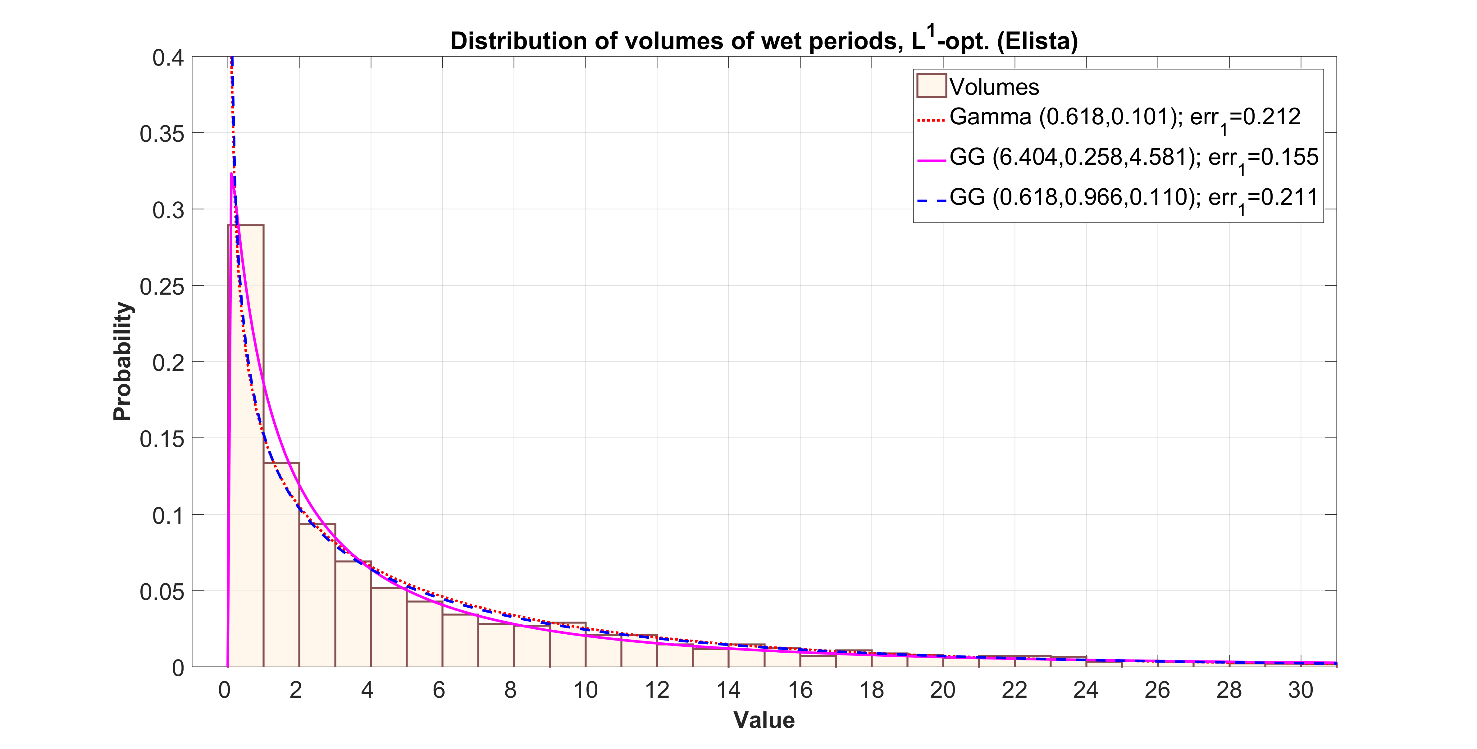
Figure 4: Approximation of the initial data distribution by optimization of $L^{1}$-metric.

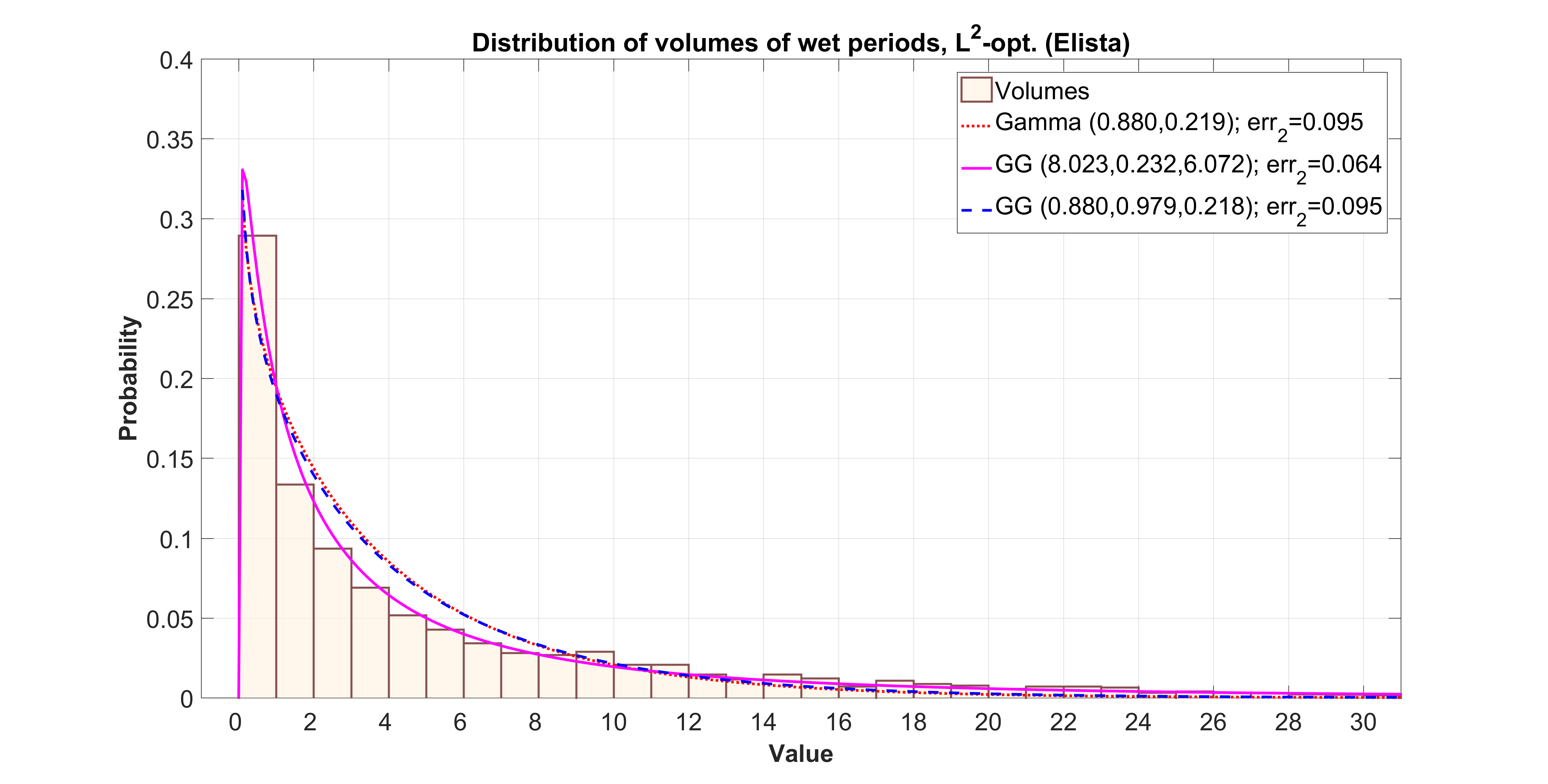
Figure 5: Approximation of the initial data distribution by optimization of $L^{2}$-metric.

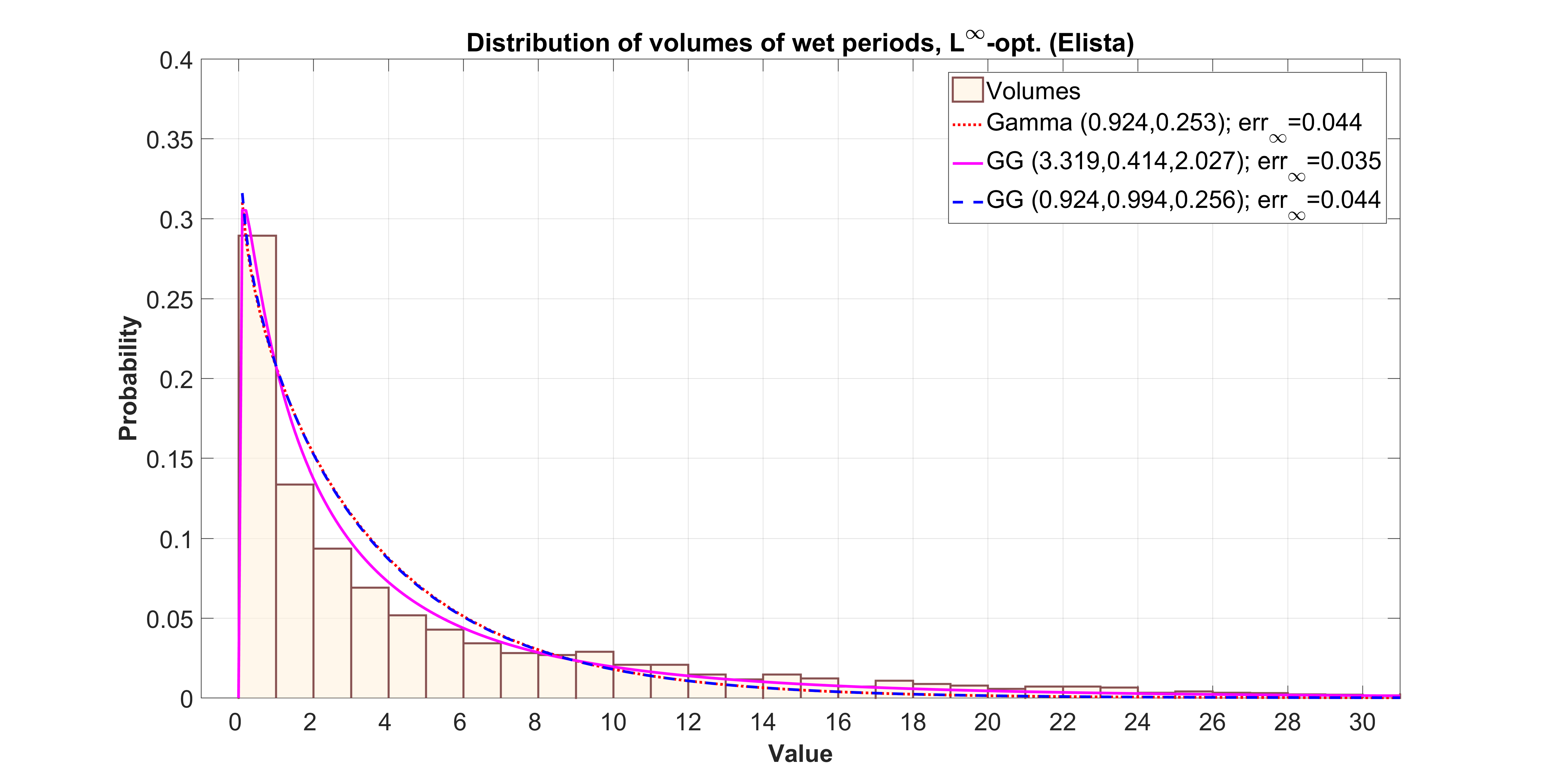
Figure 6: Approximation of the initial data distribution by optimization of $L^{\infty}$-metric.

A special MATLAB program is implemented for finding GG approximations and plotting figures. The numerical optimization is based on the simplex search method [19]. The functions for estimating values of all three unknown parameters of GG distribution or two parameters provided the shape parameter $r$ is given based on the gamma distribution model are created. The histogram and approximating probability density functions of gamma and GG distributions as well as errors in the corresponding metrics are plotted. The examples of results are shown on Figures 4–6.

They demonstrate a high quality of the approximation of the histogram of the initial data by each type of distributions. Table 2 represents approximation errors, the parameters are estimated by each of the metrics. Obviously, the results for GG distributions are better (see the bold marked items).

Table 2: Approximation errors for gamma and generalized gamma distributions, test sample.

Distribution	Error ($L^{1}$)	Error ($L^{2}$)	Error ($L^{\infty}$)
Gamma	$0{,}212$	$0{,}095$	$0{,}044$
GG	$\bf 0{,}155$	$\bf 0{,}064$	$\bf 0{,}035$
GG, fixed $r$	$0{,}211$	$0{,}095$	$0{,}044$

6 Conclusion

The classical negative binomial distribution was successfully used as a model for the number of subsequent wet days in precipitation problems for the data registered in climatically different points (see, for example, [21, 22, 23]). It was demonstrated that the fluctuations of the data with very high confidence fit the negative binomial distribution. Obviously, a more flexible GNB model could provide even better fit with the statistical data. Herewith the GG distribution can be effectively used to model aggregated data (for example, volumes accumulated over a period) and can be useful for statistical testing of hypotheses about their extremality.

Moreover, such types of mixed probability models are quite adequate for information systems (for example, in insurance [24, 25], financial mathematics [26, 27], physics [28, 29, 30], data flows [31] and many other fields). The developed functional methods for the estimation of the unknown distribution parameters can be implemented as numerical procedures in the research support system for stochastic data processing [32, 33] to analyze events in various information flows.

References

- [1] Korolev, V.Yu., Zeifman, A.I.: GG mixed Poisson distributions as mixed geometric laws and related limit theorems. arXiv:1703.07276v2 [math.PR], 11 December, 2017.
- [2] Greenwood, M., Yule, G.U. An inquiry into the nature of frequency-distributions of multiple happenings, etc.: Journal of the Royal Statistical Society. 83. 255–279 (1920)
- [3] Sichel, H.S. On a family of discrete distributions particularly suited to represent long tailed frequency data. In: Proceedings of the 3rd Symposium on Mathematical Statistics, pp. 51–97. CSIR, Pretoria (1971)
- [4] Korolev, V.Yu., Korchagin, A.Yu., Zeifman A.I.: Poisson theorem for the scheme of Bernoulli trials with random probability of success and a discrete analog of the Weibull distribution. Informatika i ee Primeneniya. 10(4), 11–20 (2016)
- [5] Stacy, E.W.: A generalization of the gamma distribution. Annals of Mathematical Statistics. 33, 1187–1192 (1962)
- [6] der Maur, A.N.F.: Statistical tools for drop size distributions: Moments and generalized gamma. Journal of the Atmospheric Sciences. 58(4), 407–418 (2001)
- [7] Nadarajah, S., Gupta, A.K.: Statistical tools for drop size distributions: Moments and generalized gamma. Mathematics and Computers in Simulation. 74(1), 1–7 (2007)
- [8] Xie, X., Liu, X.: Analytical three-moment autoconversion parameterization based on generalized gamma distribution. Journal of Geophysical Research-Atmospheres. 114, D17201 (2009)
- [9] Li, H.-C., Hong W., Wu, Y.-R., Fan, P.-Z.: An Efficient and Flexible Statistical Model Based on Generalized Gamma Distribution for Amplitude SAR Images. IEEE Transactions on Geoscience and Remote Sensing. 48(6), 2711–2722 (2010)
- [10] Li, H.-C., Hong W., Wu, Y.-R., Fan, P.-Z.: On the Empirical-Statistical Modeling of SAR Images With Generalized Gamma Distribution. IEEE Journal of Selected Topics in Signal Processing. 5(3), 386-397 (2011)
- [11] Qin, X., Zou, H., Zhou S., Ji, K.: Region-Based Classification of SAR Images Using Kullback-Leibler Distance Between Generalized Gamma Distributions. IEEE Geoscience and Remote Sensing Letters. 12(8), 1655–1659 (2015)
- [12] Sportouche, H., Nicolas, J.-M.., Tupin, F.: Mimic Capacity Of Fisher And Generalized Gamma Distributions For High-Resolution SAR Image Statistical Modeling. IEEE Journal of Selected Topics in Applied Earth Observations and Remote Sensing. 10(12), 5695–5711 (2017)
- [13] Zaninetti, L.: The Luminosity Function of Galaxies as Modeled by the Generalized Gamma Distribution. Acta Physica Polonica B. 41(4), 729-751 (2010)
- [14] Shin, J., Chang, J., Kim, N.: Statistical modeling of speech signals based on generalized gamma distribution. IEEE Signal Processing Letters. 12(3), 258–261 (2005)
- [15] Almpanidis, G., Kotropoulos, C.: Phonemic segmentation using the generalised Gamma distribution and small sample Bayesian information criterion. Speech Communication. 50(1), 38–55 (2008)
- [16] Song, K.-S.: Globally convergent algorithms for estimating generalized gamma distributions in fast signal and image processing. IEEE Transactions on Image Processing. 17(8), 1233–1250 (2008)
- [17] Huang, P.-H., Hwang, T.Y.: New moment estimation of parameters of the generalized gamma distribution using it’s characterization. Taiwanese Journal of Mathematics. 10(4), 1083–1093 (2006)
- [18] Zaks, L.M., Korolev, V.Yu.: Generalized variance gamma distributions as limit laws for random sums. Informatika i ee Primeneniya. 7(1), 105–115. (2013)
- [19] Lagarias, J.C., Reeds, J.A., Wright, M.H., Wright, P.E.: Convergence Properties of the Nelder-Mead Simplex Method in Low Dimensions. SIAM Journal of Optimization. 9(1), 112–147 (1998)
- [20] Freedman, D., Diaconis, P.Z.: On the histogram as a density estimator: theory. Zeitschrift Fur Wahrscheinlichkeitstheorie und Verwandte Gebiete. 57(4), 453–476 (1981)
- [21] Korolev, V.Yu., Gorshenin, A.K., Gulev, S.K., Belyaev, K.P., Grusho, A.A.: Statistical analysis of precipitation events. AIP Conference Proceedings. 1863, 090011 (2017)
- [22] Korolev, V.Yu., Gorshenin, A.K.: The probability distribution of extreme precipitation. Doklady Earth Sciences. 477(2), 1461–1466 (2017)
- [23] Gorshenin, A.K. Pattern-based analysis of probabilistic and statistical characteristics of precipitations. Informatika i ee Primeneniya. 11(4), 38–46 (2017)
- [24] Grandell, J.: Mixed Poisson Processes. Chapman and Hall, London (1997)
- [25] Bening, V.E., Korolev, V.Yu.: Generalized Poisson Models and Their Applications in Insurance and Finance. VSP, Utrecht (2002)
- [26] Gorshenin, A.K., Korolev, V.Yu., Zeifman, A.I., Shorgin, S.Ya., Chertok, A.V., Evstafyev, A.I., Korchagin, A.Yu.: Modelling stock order flows with non-homogeneous intensities from high-frequency data. AIP Conference Proceedings. 1558, 2394–2397 (2013)
- [27] Korolev, V.Yu., Chertok, A.V., Korchagin, A.Yu., Zeifman, A.I.: Modeling high-frequency order flow imbalance by functional limit theorems for two-sided risk processes. Applied Mathematics and Computation. 253, 224–241 (2015)
- [28] Korolev, V.Yu., Skvortsova, N.N. (eds.): Stochastic Models of Structural Plasma Turbulence. VSP, Utrecht (2006)
- [29] Batanov, G.M., Gorshenin, A.K., Korolev, V.Yu., Malakhov, D.V., Skvortsova, N.N.: The Evolution of Probability Characteristics of Low-Frequency Plasma Turbulence. Mathematical Models and Computer Simulations. 4(1), 10–25 (2012)
- [30] Gorshenin, A.K., Korolev, V.Yu., Skvortsova, N.N., Malakhov, D.V.: On non-parametric methodology of the plasma turbulence research. AIP Conference Proceedings. 1558, 2377–2380 (2013)
- [31] Gorshenin, A., Korolev, V.: Modelling of statistical fluctuations of information flows by mixtures of gamma distributions. In: Proceedings of 27th European Conference on Modelling and Simulation, pp. 569–572. Digitaldruck Pirrot GmbHP, Dudweiler (2013)
- [32] Gorshenin, A., Kuzmin, V.: On an interface of the online system for a stochastic analysis of the varied information flows. AIP Conference Proceedings. 1738, 220009 (2016)
- [33] Gorshenin, A.K., Kuzmin, V.Yu.: Research support system for stochastic data processing // Pattern Recognition and Image Analysis. 27(3), 518–524 (2017)