Low-dissipation Carnot-like heat engines at maximum efficient power

Abstract

We study the optimal performance of Carnot-like heat engines working in low dissipation regime using the product of the efficiency and the power output, also known as the efficient power, as our objective function. Efficient power function represents the best trade-off between power and efficiency of a heat engine. We find lower and upper bounds on the efficiency in case of extreme asymmetric dissipation when the ratio of dissipation coefficients at the cold and the hot contacts approaches, respectively, zero or infinity. In addition, we obtain the form of efficiency for the case of symmetric dissipation. We also discuss the universal features of efficiency at maximum efficient power and derive the bounds on the efficiency using global linear-irreversible framework introduced recently by one of the authors.

I Introduction

Carnot efficiency, $\eta_{\rm C}=1-T_{c}/T_{h}$, sets a theoretical upper bound on the efficiency of all heat engines working between two heat baths at temperatures $T_{c}$ and $T_{c}$ ($T_{c}<T_{h}$). The Carnot efficiency is attainable only in the reversible limit, whereby the processes occur so slowly that the resulting output power is zero. But, real heat engines operate at finite rates and hence produce finite power per cycle. So it is more useful to optimize the power output of the heat engines. The derivation of Curzon-Ahlborn (CA) efficiency $\eta_{CA}=1-\sqrt{1-\eta_{\rm C}}$ of an endoreversible engine Curzon and Ahlborn (1975), operating at maximum power (MP), marked the beginning of finite-time thermodynamics (FTT) de Vos (1992); Berry et al. (1999); Wu et al. (2004). In endoreversible models Curzon and Ahlborn (1975); de Vos (1985); Rubin and Andresen (1982), the work extracting part of the cycle is assumed to be internally reversible and there are no heat leaks between the heat baths. The irreversibility arises solely due to the finite rate of heat transfer between the working medium and the external heat baths. However, CA efficiency is not a universal result, and it is neither an upper nor a lower bound Van den Broeck (2005). In the linear response regime, efficiency at maximum power (EMP) comes out to be $\eta_{\rm C}/2$ for the the tight coupling condition Van den Broeck (2005). At the level of nonlinear response, Esposito et al. proved that second order term $\eta_{\rm C}^{2}/8$ is also universal if we have a left-right symmetry in addition to tight coupling condition Esposito et al. (2009).

Recently, using the assumption of low dissipation (LD), Esposito et al Esposito et al. (2010), derived upper and lower bounds for the EMP of Carnot-like heat engines. In addition, for the symmetric dissipation, they were able to reproduce the CA result. The LD models Esposito et al. (2010); Van den Broeck (2013); Schmiedl and Seifert (2008); de Tomás et al. (2012); Wang et al. (2012a); de Tomás et al. (2013); Guo et al. (2013a); Holubec and Ryabov (2015, 2016); Hernández et al. (2015); Wang and He (2012); Wang et al. (2012b); Guo et al. (2013b); Hu et al. (2013) have some advantages over the endoreversible models. It does not make use of any specific heat transfer law and also valid beyond the linear-response regime. A good comparison of LD models and endoreversible models is given in the Refs. Johal (2017a); Gonzalez-Ayala et al. (2016, 2017); Tang et al. (2018). Further, LD models were used to investigate the optimal performance of Carnot-like refrigerators de Tomás et al. (2012); Wang et al. (2012a); Hu et al. (2013), quantum heat engines Wang et al. (2012b); Guo et al. (2013b) and for the optimization of target functions other than power output de Tomás et al. (2013); Holubec and Ryabov (2015, 2016). Guo et. al. investigated the the optimal performance of LD heat engines for different types of heat cycles other than Carnot cycle Guo et al. (2013a).

But, heat engines operating at MP are not the most efficient ones and, hence, are not much economical. It has been already pointed out that actual thermal plants and heat engines should not operate at MP, but in a regime with slightly smaller power and appreciable larger efficiency Chen et al. (2001); de Vos (1992). The optimization of Omega criterion or ecological criterion Angulo-Brown (1991); Hernández et al. (2001); Singh and Johal (2017) and efficient power criterion Stucki (1980); Yan and Chen (1996); Yilmaz (2006) falls in such a regime. They pay equal attention to both power output and efficiency Arias-Hernandez et al. (2009). In this work, we investigate the optimization of efficient power criterion for a Carnot-like engine working in LD regime.

Efficient power criterion $P_{\eta}=\eta P$ represents the best compromise between the efficiency and power output of a heat engine. In was introduced by Stucki Stucki (1980) in the context of linear-irreversible thermodynamics (LIT) while studying the mitochondrial energetic processes. Later the idea was extended to the regime of FTT by Yan and Chen Yan and Chen (1996) and given the so-called name efficient power by Yilmaz Yilmaz (2006). It is also shown that the efficient power criterion is also well suited to study the optimization of steady and non-steady electric energy converters Valencia-Ortega (2016), thermionic generator Chen et al. (2017) and biological systems Stucki (1980); Arias-Hernandez et al. (2008); Chimal et al. (2017). For some naturally designed biological systems, maximum efficient power (MEP) conditions may lead to more efficient engines than those at maximum Omega function (MOF) or ecological function Chimal et al. (2017).

In this paper, we analyse the optimal performance of general class of LD Carnot-like heat engines using efficient power function as the objective function. In Sec.II, we discuss model of LD heat engine undergoing Carnot cycle. In Sec. III, we find the general expression for EMEP and obtain lower and upper bound on the efficiency. We also discuss universal features of EMEP in this section. Sec. IV is devoted to the comparison of rates of dissipation at hot and cold contacts for three different objective functions. In Sec. V, using a different optimization scheme, we obtain the same bounds on the EMEP as obtained for LD heat engines. We conclude in Sec. VI by highlighting the key results.

II Model of low-dissipation Carnot engine

As in the case of usual Carnot cycle, heat cycle in our case consists of two adiabatic and two isothermal steps. Adiabatic steps are assumed to be instantaneous and there is no entropy production along these branches. Let $t_{h}$ and $t_{c}$ be the time durations of the isothermal branches during which the system remains in contact with the hot and cold reservoirs respectively. During the heat exchange process with the hot (cold) bath, the change in entropy of the system can be split into two parts as follows

$$\Delta S_{j}=\Delta S_{j}^{r}+\Delta S_{j}^{ir},\qquad j=h,c$$ (1)

where $\Delta S_{j}^{r}$ is change in entropy of the system due to reversible heat transfer and $\Delta S_{j}^{ir}$ accounts for irreversible entropy production during the process. The first term is $Q_{h}/T_{h}$ for the heat absorbed from the hot reservoir at temperature $T_{h}$ and $Q_{c}/T_{c}$ for the heat transferred to cold reservoir at temperature $T_{c}$. In low dissipation limit, it is assumed that irreversible entropy production $\Delta S_{j}^{ir}$ during the heat transfer step is inversely proportional to the time duration for which the system remains in contact with the bath. Hence entropy production along the isothermal branch is given by $\Delta S_{j}^{ir}=\Sigma_{j}/t_{j}$, ($j=h,c$). Here $\Sigma_{h}$ and $\Sigma_{c}$ are dissipation coefficients, containing the information about the irreversibilities induced in the model as we deviate away from the reversible limit. It is self evident that the cycle approaches reversible limit as $t_{h}\rightarrow\infty$ and $t_{c}\rightarrow\infty$. Thus, at hold and cold contacts, we have respectively

$$\Delta S_{h} = \frac{Q_{h}}{T_{h}}+\frac{\Sigma_{h}}{t_{h}},$$ (2)

$$\Delta S_{c} = -\frac{Q_{c}}{T_{c}}+\frac{\Sigma_{c}}{t_{c}},$$ (3)

where $Q_{h},Q_{c}>0$. Since after undergoing the full cycle, the system returns to its initial state, the total entropy change in the whole cycle is zero: $\Delta S_{h}+\Delta S_{c}=0$. Therefore we have $\Delta S_{h}=-\Delta S_{c}=\Delta S>0$. Then the amount of heat exchanged with each reservoir can be written as

$$Q_{h} = T_{h}\left(\Delta S-\frac{\Sigma_{h}}{t_{h}}\right)\equiv T_{h}(\Delta S-x_{h}\Sigma_{h}),$$ (4)

$$Q_{c} = T_{c}\left(\Delta S+\frac{\Sigma_{c}}{t_{c}}\right)\equiv T_{c}(\Delta S+x_{c}\Sigma_{c}),$$ (5)

where we have used $x_{h}\equiv 1/t_{h}$ and $x_{c}\equiv 1/t_{h}$ for our convenience. The work extracted in a cycle with time period $t=t_{c}+t_{h}$ is $W=Q_{h}-Q_{c}$. So the efficiency $\eta$ and average output power $P$ per cycle is defined as

$$\eta=\frac{W}{Q_{h}}=1-\frac{Q_{h}}{Q_{c}}=1-\frac{T_{c}(\Delta S+x_{c}\Sigma_{c})}{T_{h}(\Delta S-x_{h}\Sigma_{h}},$$ (6)

$$P=\frac{Q_{h}-Q_{c}}{t_{h}+t_{c}}\equiv\frac{(Q_{h}-Q_{c})x_{h}x_{c}}{x_{c}+x_{h}}$$ (7)

III Efficient power in low dissipation regime

To study the optimal performance of a low dissipation Carnot engine, we will use efficient power $P_{\eta}=\eta P$ as the target function. Here, the efficient power represents the best compromise between the efficiency and average power of the engine. Using Eqs. (6) and (7) in the expression for $P_{\eta}$, we have

$$P_{\eta}=\eta P=\frac{(Q_{h}-Q_{c})^{2}}{Q_{h}}\frac{x_{c}x_{h}}{x_{c}+x_{h}}.$$ (8)

Setting the partial derivatives of $P_{\eta}$ with respect to $x_{c}$ and $x_{h}$ equal to zero, we have respectively the following two equations:

$$\frac{(Q_{h}-Q_{c})^{2}}{Q_{h}}x_{h}=2T_{c}\Sigma_{c}(x_{c}+x_{h})x_{c}\left[1-\frac{T_{c}(\Delta S+x_{c}\Sigma_{c})}{T_{h}(\Delta S-x_{h}\Sigma_{h})}\right],$$ (9)

and

$$\frac{(Q_{h}-Q_{c})^{2}}{Q_{h}}x_{c}=T_{h}\Sigma_{h}(x_{c}+x_{h})x_{h}\left[1-\frac{T_{c}^{2}}{T_{h}^{2}}\frac{(\Delta S+x_{c}\Sigma_{c})^{2}}{(\Delta S-x_{h}\Sigma_{h})^{2}}\right].$$ (10)

Using Eqs. (4) and (5) in Eqs. (9) and (10), we solve for $x_{h}$ and get the following expression (see Appendix A) for $x_{h}$

$$x_{h}=-\frac{\Delta SN}{8\Sigma_{h}B}-\frac{1}{2}\sqrt{K}-\frac{1}{2}\sqrt{K^{\prime}-\frac{1}{4\sqrt{K}}\left[\frac{\Delta S^{3}}{\Sigma_{h}^{3}}\left(\frac{12\eta_{\rm C}\Sigma_{h}}{B}-\frac{N^{3}}{8B^{3}}+\frac{MN}{2B^{2}}\right)\right]}$$ (11)

where we used the following notation

$$K = \frac{\Delta S^{2}}{\Sigma_{h}^{2}}\left[\frac{N^{2}}{16B^{2}}-\frac{M}{6B}+\frac{(A+\sqrt{A^{2}-4A^{\prime 3}})^{1/3}}{12\times 2^{1/3}\Sigma_{h}B}+\frac{\Sigma_{h}T}{6\times 2^{2/3}B(A+\sqrt{A^{2}-4A^{\prime 3}})^{1/3}}\right],$$

$$K^{\prime} = \frac{\Delta S^{2}}{\Sigma_{h}^{2}}\left[\frac{N^{2}}{8B^{2}}-\frac{M}{3B}-\frac{(A+\sqrt{A^{2}-4A^{\prime 3}})^{1/3}}{12\times 2^{1/3}\Sigma_{h}B}-\frac{\Sigma_{h}T}{6\times 2^{2/3}B(A+\sqrt{A^{2}-4A^{\prime 3}})^{1/3}}\right],$$

$$N = \Sigma_{h}\left[(1-\eta_{\rm C})(6-\eta_{\rm C})\gamma-6\right],$$

$$B = \Sigma_{h}\left[-(1-\eta_{\rm C})\gamma+1\right],$$

$$M = \Sigma_{h}\left[-3(1-\eta_{\rm C})(3-\eta_{\rm C})\gamma+(4\eta_{\rm C}+9)\right],$$

$$T = \Sigma_{h}^{2}[9(1-\eta_{\rm C})^{2}(3-\eta_{\rm C})^{2}\gamma^{2}-6(1-\eta_{\rm C})(3-2\eta_{\rm C})(9-5\eta_{\rm C})\gamma+(9-8\eta_{\rm C})^{2}],$$

$$A = 2M^{3}\Sigma_{h}^{3}+108\eta_{\rm C}\Sigma_{h}^{4}MN+108\eta_{\rm C}^{2}\Sigma_{h}^{4}N^{2}+3888\eta_{\rm C}^{2}\Sigma_{h}^{5}B-288\eta_{\rm C}^{2}\Sigma_{h}^{4}MB,$$

$$A^{\prime} = M^{2}\Sigma_{h}^{2}+36\eta_{\rm C}\Sigma_{h}^{3}N+48\eta_{\rm C}^{2}\Sigma_{h}^{3}B.$$ (12)

In the above equations, we have introduced the parameter $\gamma=\Sigma_{c}/\Sigma_{h}$. Now we seek the form of efficiency at maximum efficienct power (EMEP) $\eta^{*}=W/Q_{h}$, which is found to be (see Appendix B)

$$\eta^{*}=\frac{2\eta_{\rm C}}{3-2x_{h}\Sigma_{h}/\Delta S}.$$ (13)

Using Eqs. (11) and (12) in Eq. (13), we can obtain a closed-form expression for EMEP. The resulting form is too lengthy to be reproduced here. However, a couple of points about this expression need to be noted. Firstly, it depends only upon Carnot efficiency $\eta_{\rm C}$ and parameter $\gamma$. For some limiting cases, it reduces to well known forms for the efficiency obtained in literature. In the extreme asymmetric limit $\gamma\rightarrow 0$, the EMEP converges to the upper bound $\eta_{+}=(3-\sqrt{9-8\eta_{\rm C}})/2$, while for $\gamma\rightarrow\infty$, it reduces to the lower bound $\eta_{-}=2\eta_{\rm C}/3$. Thus

$$\eta_{-}\equiv\frac{2}{3}\eta_{\rm C}\leq\eta^{*}\leq\frac{1}{2}(3-\sqrt{9-8\eta_{\rm C}})\equiv\eta_{+}.$$ (14)

These upper and lower bounds on the efficiency were previously obtained by Holubec and Ryabov Holubec and Ryabov (2015) for the case of overdamped brownian particle undergoing a Carnot-like cycle using the framework of stochastic thermodynamics Schmiedl and Seifert (2008).

We pay special attention to the case of symmetric dissipation in which $\Sigma_{c}=\Sigma_{h}$, or $\gamma=1$. Under this condition, Eq. (13) reduces to

$$\eta_{\rm sym}=1-\frac{1}{4}(1-\eta_{\rm C})\left(1+\sqrt{1+\frac{8}{1-\eta_{\rm C}}}\right).$$ (15)

The same result was obtained in Refs. Yan and Chen (1996); Yilmaz (2006) for the endoreversible model of Carnot heat engine operating at MEP, under the tight-coupling condition. We expand Eq. (15) in Taylor’s series near equilibrium to reveal universal features of the EMEP.

$$\eta_{sym}=\frac{2}{3}\eta_{\rm C}+\frac{2}{27}\eta_{\rm C}^{2}+O(\eta_{\rm C}^{3}).$$ (16)

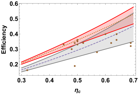
Figure 1: (Color online) Comparison of the bounds on efficiency with observed data. Red curves show the bounds for the EMEP. Gray lines represents the same for the EMP Esposito et al. (2010). Brown circles represent the observed efficiencies of various power plants as analyzed in Refs. Esposito et al. (2010); Holubec and Ryabov (2015); Johal (2017b). Dashed and dotted lines stand for $\eta_{\rm CA}$ and $\eta_{\rm sym}$ respectively.

The first two terms in the above equation were also derived for the EMEP of a nonlinear irreversible heat engine Zhang et al. (2017) working in strong coupling limit under the symmetric condition by using master equation model Esposito et al. (2009); Zhang et al. (2016). In Ref. Zhang et al. (2017), it is also shown that EMEP is given by $2\eta_{\rm C}/3$ in linear response regime. Hence, we confirm that universal features of efficiency Esposito et al. (2009); Zhang et al. (2016); Singh and Johal are not exclusive to the conditions of MP and MOF but also extend to the engines operating in MEP regime.

IV Rates of dissipation

Now we compare the average rates of dissipation for LD heat engines under optimal working conditions for power output, efficient power function and Omega ($\Omega$) function. In general, the average rates of dissipation for the LD model, at hot and cold contacts are given by Johal (2017a):

$$\mathcal{D}_{h}^{(f)}=\frac{T_{h}\Sigma_{h}}{t_{h}^{2}}\equiv T_{h}\Sigma_{h}x_{h}^{2},$$ (17)

$$\mathcal{D}_{c}^{(f)}=\frac{T_{c}\Sigma_{c}}{t_{c}^{2}}\equiv T_{c}\Sigma_{c}x_{c}^{2},$$ (18)

where $f(\equiv P,\;P_{\eta},\;\Omega)$ is the function being optimized. In case of LD engines operating at maximum power, the relation between $x_{h}$ and $x_{c}$ is given by Esposito et al. (2010)

$$\frac{x_{h}}{x_{c}}=\sqrt{\frac{T_{c}\Sigma_{c}}{T_{h}\Sigma_{h}}},$$ (19)

from which it follows that the average rates of dissipation at two thermal contacts are equal:

$$\mathcal{D}_{c}^{(P)}=\mathcal{D}_{h}^{(P)}.$$ (20)

Similarly for the case of maximum $\Omega$ function, we have de Tomás et al. (2013)

$$\frac{x_{c}}{x_{h}}=\sqrt{\frac{\Sigma_{h}(2-\eta_{\rm C})}{2\Sigma_{c}(1-\eta_{\rm C})}}.$$ (21)

So, we obtain

$$\mathcal{D}_{c}^{(\Omega)}=\mathcal{D}_{h}^{(\Omega)}\left(1-\frac{\eta_{\rm C}}{2}\right).$$ (22)

Since the factor $(1-\eta_{\rm C}/2)$ is always smaller than 1, the rate of dissipation is higher at the hot contact. Now we find the relation between rates of dissipation for the case of LD engines operating at MEP. From Eqs. (32) and (35), we have

$$\frac{x_{c}}{x_{h}}=\sqrt{\frac{\Sigma_{h}(2-\eta^{*})}{2\Sigma_{c}(1-\eta_{\rm C})}},$$ (23)

which can be solved to give

$$\mathcal{D}_{c}^{(P_{\eta})}=\mathcal{D}_{h}^{(P_{\eta})}\left(1-\frac{\eta^{*}}{2}\right).$$ (24)

Comparing Eqs. (20), (22) and (24), it is clear that ratio of cold to hot dissipation is smallest in the case of Omega function:

$$\frac{\mathcal{D}_{c}^{(\Omega)}}{\mathcal{D}_{h}^{(\Omega)}}<\frac{\mathcal{D}_{c}^{(P_{\eta})}}{\mathcal{D}_{h}^{(P_{\eta})}}<\frac{\mathcal{D}_{c}^{(P)}}{\mathcal{D}_{h}^{(P)}}=1.$$ (25)

Here, we emphasize that as the ratio of the rates of dissipation at the cold and the hot ends decreases, the efficiency of the engine increases, which is clear from the fact that in strong coupling limit, engines operating at MOF are the most efficient ones and the engines working in the MP regime are the least efficient Arias-Hernandez et al. (2009). We also note that in the cases of MP and MOF, the ratio of rates of dissipation is independent of dissipation constants $\Sigma_{c}$ and $\Sigma_{h}$, whereas for MEP it depends upon $\gamma$ as the general form of EMEP is a function of $\gamma$.

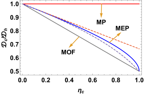
Figure 2: (Color online) Solid lines represent the ratio of the rates of dissipation at cold and hot contacts of the indicated function under symmetric dissipation, $\gamma=1$. Dashed upper and lower curves represent the ratio $\mathcal{D}_{c}^{(P_{\eta})}/\mathcal{D}_{h}^{(P_{\eta})}$ for the extreme asymmetric dissipation $\gamma\rightarrow\infty$ and $\gamma\rightarrow 0$, respectively.

V Global linear-irreversible principle

We noted in the above that the bounds on EMEP have also been obtained with other models such as the endoreversible model. The similarities and differences between endoreversible and LD models have been discussed recently Johal (2017a); Gonzalez-Ayala et al. (2016, 2017); Tang et al. (2018). While different such models assume a particular functional form or a mechanism for irreversible entropy generation, we discuss in the following a different formulation that has been recently proposed by one of the authors Johal (2018) and show that the same lower and upper bounds as obtained in Eq. (14) and (15) can be obtained using a different optimization scheme. In this so-called global linear-irreversible principle (GLIP) framework, we do not assume stepwise details of the cycle. Rather, the validity of LIT is assumed globally, i.e., for the complete cycle. Here, the thermal machine is considered as an irreversible channel with an effective heat conductivity $\lambda$, with an associated passage of a mean heat $\bar{Q}$ from hot to cold reservoir in the total cycle time $\tau$. Thereby, the relation between total cycle time $\tau$ and $\bar{Q}$ is given by Johal (2018)

$$\tau=\frac{\bar{Q}^{2}}{\lambda\Delta S_{\rm tot}},$$ (26)

where $\Delta S_{\rm tot}=Q_{c}/T_{c}-Q_{h}/T_{h}$, is the total entropy generated per cycle. Using the basic definitions and Eq. (26), the average efficient power is given by

$$P_{\eta}=\eta\frac{W}{\tau}=\frac{\lambda(Q_{h}-Q_{c})^{2}}{Q_{h}\bar{Q}^{2}}\Delta S_{\rm tot}=\frac{\lambda(Q_{h}-Q_{c})^{2}}{Q_{h}\bar{Q}^{2}}\left(\frac{Q_{c}}{T_{c}}-\frac{Q_{h}}{T_{h}}\right).$$ (27)

Defining $\nu=Q_{c}/Q_{h}$, we can rewrite Eq. (27) in terms of $\eta_{\rm C}$ and $\nu$:

$$P_{\eta}=\frac{\lambda}{T_{c}}(1-\nu)(\nu+\eta_{\rm C}-1)\frac{{Q}^{2}_{h}}{\bar{Q}^{2}}.$$ (28)

Now, in order to optimize the above objective function, we have to specify the form of $\bar{Q}$ which is assumed to be a mean value lying in the range $Q_{c}\leq\bar{Q}\leq Q_{h}$. We will discuss here only the extreme cases. Substituting $\bar{Q}=Q_{h}$ in Eq. (28) and optimizing with respect to $\nu$, EMEP comes out to be $\eta_{-}=2\eta_{\rm C}/3$. Similarly, for $\bar{Q}=Q_{c}$, the form of EMEP is $\eta_{+}=(3-\sqrt{9-8\eta_{\rm C}})/2$. Alternately, if we use the geometric mean $\bar{Q}=\sqrt{Q_{c}Q_{h}}$, the optimization of Eq. (28) yields the EMEP as in Eq. (15).

VI Conclusions

We have discussed the efficiency of a LD heat engine operating at MEP. In the limit of extremely asymmetric dissipation, we are able to obtain the lower and upper bounds on the efficiency of the engine, as well as the expression $\eta_{sym}$ for the symmetric case. The universal features of EMEP are highlighted. We also note that ratio of average dissipation rates at cold and hot contacts depends upon $\gamma$, see Eq. (24), whereas in the case of MP and MOF, the same ratio is independent of $\gamma$, see Eqs. (20) and (22). The derivation of forms of EMEP, similar to those obtained for LD Carnot-like engines, using the global principle of LIT, confirms the validity of our analysis.

Although the real power plants do not operate in a Carnot cycle, and the assumption of low dissipation may not be valid for them, it is compelling to compare the upper and lower bounds with the observed efficiencies. In Fig. 1, we have compared the observed data with the bounds obtained for LD engines operating at MP and MEP. Although not shown in Fig. 1, it is important to know that the area between the lower and upper bounds of MOF does not contain any observed data points Holubec and Ryabov (2015), whereas five and eight data points respectively lie within the areas bounded by the lower and upper bounds of EMEP and EMP. However, it is interesting to observe that the density of points (number of data points per unit area between the upper and lower bounds for the respective objective function shown in Fig. 1), is higher in the case of MEP criterion than for MP.

Appendix A

Substituting the values of $Q_{h}$ and $Q_{c}$ from Eqs. (4) and (5) into the Eqs. (9) and (10) and then adding, we have

$$T_{h}(\Delta S-x_{h}\Sigma_{h})-2T_{c}(\Delta S+x_{c}\Sigma_{c})-2T_{c}x_{c}\Sigma_{c}\left[1-\frac{T_{c}(\Delta S+x_{c}\Sigma_{c})}{T_{h}(\Delta S-x_{h}\Sigma_{h})}\right]$$

$$+T_{h}\left[1-\frac{T_{c}^{2}(\Delta S+x_{c}\Sigma_{c})^{2}}{T_{h}^{2}(\Delta S-x_{h}\Sigma_{h})}\right]-x_{h}\Sigma_{h}T_{h}\left[1-\frac{T_{c}^{2}(\Delta S+x_{c}\Sigma_{c})^{2}}{T_{h}^{2}(\Delta S-x_{h}\Sigma_{h})^{2}}\right]=0.$$ (29)

Further writing the above equation in terms of $\eta_{\rm C}=1-T_{c}/T_{h}$, we have

$$\Delta S -2x_{h}\Sigma_{h}-4(1-\eta_{\rm C})x_{c}\Sigma_{c}-2(1-\eta_{\rm C})\Delta S$$ (30)

$$+2(1-\eta_{\rm C})^{2}x_{c}\Sigma_{c}\frac{\Delta S+x_{c}\Sigma_{c}}{\Delta S-x_{h}\Sigma_{h}}+\Delta S(1-\eta_{\rm C})^{2}\frac{(\Delta S+x_{c}\Sigma_{c})^{2}}{(\Delta S-x_{h}\Sigma_{h})^{2}}=0.$$

Solving Eq. (30) for $x_{c}$, we have

$$x_{c}=\frac{1}{\Sigma_{c}(1-\eta_{\rm C})}\left[\frac{\Delta S^{2}\eta_{\rm C}}{3\Delta S-2x_{h}\Sigma_{h}}-x_{h}\Sigma_{h}\right].$$ (31)

Dividing Eqs. (9) and (10) and writing in terms of $\eta_{\rm C}$, we get

$$\frac{x_{c}^{2}}{x_{h}^{2}}=\frac{\Sigma_{h}}{2\Sigma_{c}}\left[\frac{\Delta S+x_{c}\Sigma_{c}}{\Delta S-x_{h}\Sigma_{h}}+\frac{1}{1-\eta_{\rm C}}\right].$$ (32)

Again solving Eq. (32) for $x_{c}$ and writing in terms of $\gamma$, we have

$$x_{c} = \frac{1}{4(1-\eta_{\rm C})\Sigma_{c}(\Delta S-x_{h}\Sigma_{h})}\bigg{[}\gamma x_{h}^{2}\Sigma_{h}^{2}(1-\eta_{\rm C})-x_{h}\Sigma_{h}\sqrt{\gamma(1-\eta_{\rm C})}$$ (33)

$$\times\sqrt{8\Delta S^{2}(2-\eta_{\rm C})-8\Delta Sx_{h}\Sigma_{h}(3-\eta_{\rm C})+\gamma x_{h}^{2}\Sigma_{h}^{2}(1-\eta_{\rm C})+8x_{h}^{2}\Sigma_{h}^{2}}\bigg{]}$$

Eliminating $x_{c}$ from Eqs. (31) and (33), we have the final expression for $x_{h}$ as given by Eq. (11).

Appendix B

Efficiency of the engine is given by:

$$\eta=\frac{W}{Q_{h}}=1-\frac{Q_{c}}{Q_{h}}.$$ (34)

Using Eq. (4) and (5) and writing in terms of $\eta_{\rm C}$, the expression for efficiency becomes

$$\eta=1-(1-\eta_{\rm C})\frac{\Delta S+x_{c}\Sigma_{c}}{\Delta S-x_{h}\Sigma_{h}}.$$ (35)

Rearranging the terms in Eq. (31), we obtain under conditions of MEP

$$(\Delta S+x_{c}\Sigma_{c})(1-\eta_{\rm C})=\frac{\Delta S^{2}\eta_{\rm C}}{3\Delta S-2x_{h}\Sigma_{h}}+\Delta S-x_{h}\Sigma_{h}-\Delta S\eta_{\rm C}.$$ (36)

Substituting Eq. (36) in Eq. (35), we obtain following form of efficiency

$$\eta^{*}=\frac{2\eta_{\rm C}}{3-2x_{h}\Sigma_{h}/\Delta S}.$$ (37)

.

References

- Curzon and Ahlborn (1975) F. L. Curzon and B. Ahlborn, Am. J. Phys. 43, 22 (1975).
- de Vos (1992) A. de Vos, Endoreversible Thermodynamics of Solar Energy Conversion (Oxford University Press, Oxford, UK, 1992).
- Berry et al. (1999) R. S. Berry, V. Kazakov, S. Sieniutycz, Z. Szwast, and A. M. Tsirlin, Thermodynamic Optimization of Finite-Time Processes (Wiley, Chichester, UK, 1999).
- Wu et al. (2004) C. Wu, L. Chen, and J. Chen, Advances in Finite-Time Thermodynamics: Analysis and Optimization (Nova Science, New York, 2004).
- de Vos (1985) A. de Vos, Am. J. Phys. 53, 57 (1985).
- Rubin and Andresen (1982) M. H. Rubin and B. Andresen, J. Appl. Phys. 53, 1 (1982).
- Van den Broeck (2005) C. Van den Broeck, Phys. Rev. Lett. 95, 190602 (2005).
- Esposito et al. (2009) M. Esposito, K. Lindenberg, and C. Van den Broeck, Phys. Rev. Lett. 102, 130602 (2009).
- Esposito et al. (2010) M. Esposito, R. Kawai, K. Lindenberg, and C. Van den Broeck, Phys. Rev. Lett. 105, 150603 (2010).
- Van den Broeck (2013) C. Van den Broeck, EPL (Europhysics Letters) 101, 10006 (2013).
- Schmiedl and Seifert (2008) T. Schmiedl and U. Seifert, EPL (Europhysics Letters) 81, 20003 (2008).
- de Tomás et al. (2012) C. de Tomás, A. C. Hernández, and J. M. M. Roco, Phys. Rev. E 85, 010104 (2012).
- Wang et al. (2012a) Y. Wang, M. Li, Z. C. Tu, A. C. Hernández, and J. M. M. Roco, Phys. Rev. E 86, 011127 (2012a).
- de Tomás et al. (2013) C. de Tomás, J. M. M. Roco, A. C. Hernández, Y. Wang, and Z. C. Tu, Phys. Rev. E 87, 012105 (2013).
- Guo et al. (2013a) J. Guo, J. Wang, Y. Wang, and J. Chen, Phys. Rev. E 87, 012133 (2013a).
- Holubec and Ryabov (2015) V. Holubec and A. Ryabov, Phys. Rev. E 92, 052125 (2015).
- Holubec and Ryabov (2016) V. Holubec and A. Ryabov, J. Stat. Mech. Theory Exp. 2016, 073204 (2016).
- Hernández et al. (2015) A. C. Hernández, A. Medina, and J. M. M. Roco, New J. Phys. 17, 075011 (2015).
- Wang and He (2012) J. Wang and J. He, Phys. Rev. E 86, 051112 (2012).
- Wang et al. (2012b) J. Wang, J. He, and Z. Wu, Phys. Rev. E 85, 031145 (2012b).
- Guo et al. (2013b) J. Guo, J. Wang, Y. Wang, and J. Chen, J. Appl. Phys. 113, 143510 (2013b).
- Hu et al. (2013) Y. Hu, F. Wu, Y. Ma, J. He, J. Wang, A. C. Hernández, and J. M. M. Roco, Phys. Rev. E 88, 062115 (2013).
- Johal (2017a) R. S. Johal, Phys. Rev. E 96, 012151 (2017a).
- Gonzalez-Ayala et al. (2016) J. Gonzalez-Ayala, A. C. Hernández, and J. M. M. Roco, J. Stat. Mech. Theory Exp. 2016, 073202 (2016).
- Gonzalez-Ayala et al. (2017) J. Gonzalez-Ayala, J. M. M. Roco, A. Medina, and A. C. Hernández, Entropy 19, 182 (2017).
- Tang et al. (2018) F. R. Tang, R. Zhang, H. Li, C. N. Li, W. Liu, and B. Long, Eur. Phys. J. Plus 133, 176 (2018).
- Chen et al. (2001) J. Chen, Z. Yan, G. Lin, and B. Andresen, Energy Convers. and Manage. 42, 173 (2001).
- Angulo-Brown (1991) F. Angulo-Brown, J. Appl. Phys. 69, 7465 (1991).
- Hernández et al. (2001) A. C. Hernández, A. Medina, J. M. M. Roco, J. A. White, and S. Velasco, Phys. Rev. E 63, 037102 (2001).
- Singh and Johal (2017) V. Singh and R. S. Johal, Entropy 19, 576 (2017).
- Stucki (1980) J. W. Stucki, Eur. J. Biochem. 109, 269 (1980).
- Yan and Chen (1996) Z. Yan and J. Chen, Phys. Lett. A 217, 137 (1996).
- Yilmaz (2006) T. Yilmaz, J. Energy Inst. 79, 38 (2006).
- Arias-Hernandez et al. (2009) L. A. Arias-Hernandez, M. A. Barranco-Jiménez, and F. Angulo-Brown, J. Energy Inst. 82, 223 (2009).
- Valencia-Ortega (2016) L. Valencia-Ortega, G. Arias-Hernandez, J.Non-Equilib. Thermodyn. 42, 187 (2016).
- Chen et al. (2017) L. Chen, Z. Ding, J. Zhou, W. Wang, and F. Sun, Eur. Phys. J. Plus 132, 293 (2017).
- Arias-Hernandez et al. (2008) L. A. Arias-Hernandez, F. Angulo-Brown, and R. T. Paez-Hernandez, Phys. Rev. E 77, 011123 (2008).
- Chimal et al. (2017) J. C. Chimal, N. Sánchez, and P. Ramírez, Journal of Physics: Conference Series 792, 012082 (2017).
- Johal (2017b) R. S. Johal, Eur. Phys. J. Spec. Top. 226, 489 (2017b).
- Zhang et al. (2017) Y. Zhang, J. Guo, G. Lin, and J. Chen, J. Non-Equilib. Thermodyn. 42, 253 (2017).
- Zhang et al. (2016) Y. Zhang, C. Huang, G. Lin, and J. Chen, Phys. Rev. E 93, 032152 (2016).
- (42) V. Singh and R. S. Johal, J. Stat. Mech.: Theory and Expt., accepted for publication (2018); arXiv:1805.03856 .
- Johal (2018) R. S. Johal, EPL (Europhysics Letters) 121, 50009 (2018).