DGLAP evolution for DIS diffraction production of high masses.

Abstract

In this paper we develop the DGLAP evolution for the system of produced gluons in the process of diffractive production in DIS, directly from the evolution equation in Color Glass Condensate approach. We are able to describe the available experimental data with small value of the QCD coupling ($\bar{\alpha}_{S}\approx 0.1$). We conclude that in diffractive production, we have a dilute system of emitted gluons and in the order to describe them, we need to develop the next-to-leading order approach in perturbative QCD.

I Introduction.

In this paper we continue to re-visit the process of diffractive production in the deep inelastic scattering in the framework of CGC/saturation approach (see Ref.KOLEB for review). In this approach the diffraction production is characterized by two new scales (two saturation momenta): $Q_{s}\left(Y-Y_{0},Y_{0}\right)$, which describes the dense system of produced gluons (see Fig. 1-a) and $Q_{s}\left(Y_{0}\right)$, which corresponds to the dense system of gluons that is responsible for $N_{el}$ (see Fig. 1-b). The equations, that govern the emission of gluons in this process, were proven long ago KOLE (see also Ref.HWS ; HIMST ; KLW ) but, they have not been investigated carefully for almost two decades. The efforts of high energy community were concentrated on simple models in which the diffractive production of quark-antiquark pair and one additional gluon has been considered (see Refs.GBKW ; GOLEDD ; SATMOD0 ; KOML ; MUSCH ; MASC ; MAR ; KLMV ). The successful description of the old experimental data led to an elusive impression, that it is not necessary to investigate the dense system of produced gluons in this process. In the previous paper CLMP we developed the saturation model, in which we describe the dense system of produced gluons. However, the comparison with the experimental data shows, that we failed to describe the data in spite of a number of the fitting parameters in the model. Based on this experience, we wish to study the emission of gluons in the DGLAP evolution with the hope, that the experimental data at small $\beta$ (see Fig. 1) can be interpreted as the production of a rather dense system of gluons, which is not in the saturation region, but approaching it. In other words, we wish to search the DGLAP evolution for dipole sizes for which $r^{2}\,Q^{2}_{s}\left(Y-Y_{0},Y_{0}\right)\,\,<\,\,1$. On the other hand, we will show that $r^{2}\,Q^{2}_{s}\left(Y_{0}\right)\,\sim\,1$ contribute to the elastic amplitude, which means that we have to take into account the saturation of gluons in the structure of $N_{el}$ in Fig. 1-b. Bearing this in mind we develop the DGLAP approach in the coordinate representation directly from the equations of Ref.KOLE .

The DGLAP evolution has been discussed (see for example, Ref.DGLAPOLD and reference therein) but mostly, using the Ingelman-Schlein factorization INSC and reducing the evolution of the diffractive structure function to the DGLAP equation for the Pomeron structure function. In this paper we take a completely different approach based on the evolution equation for the diffractive cross section of Ref.KOLE , in which we do not introduce the so called soft Pomeron and its structure.

The paper is organized as follows. In the next section we give a brief review of the energy evolution of the processes of the diffractive production in DIS, which have been derived in CGC/saturation approach (see Refs.KOLEB ; KOLE ). In section 3 we solve these equation in double log approximation (DLA) in the kinematic region where $r^{2}Q^{2}_{s}\left(Y_{0},b\right)\ll\,1$ and show that this solution can describe the experimental data. In section 4 we continue to discuss the DLA and expand it to the region $r^{2}Q^{2}_{s}\left(Y_{0},b\right)\,\leq\,1$. We put our main attention on fixing the initial conditions for the DLA equation. In section 5 we present the DGLAP evolution equation for the diffractive reduced cross sections. In the conclusions we summarize our results.

II The CGC/saturation equations for DIS diffractive productions

A sketch of the process of diffraction production in DIS is shown in Fig. 1-a, from this figure one can see that the main formula he form

$$\sigma^{\rm diff}(Y,Y_{0},Q^{2})\,\,\,=\,\,\int\,\,d^{2}r_{\perp}\int\,dz\,\,|\Psi^{\gamma^{*}}(Q^{2};r_{\perp},z)|^{2}\,\,\sigma_{\rm dipole}^{diff}(r_{\perp},Y,Y_{0})\,,$$ (1)

where $Y=\ln\left(1/x_{Bj}\right)$ and $Y_{0}$ is the minimum rapidity gap for the diffraction process (see Fig. 1-b). In other words, we consider diffraction production, in which all produced hadrons have rapidities larger than $Y_{0}$. For $\sigma_{\rm dipole}^{diff}(r_{\perp},Y,Y_{0})$ we have a general expression

$$\sigma_{\rm dipole}^{diff}(r_{\perp},Y,Y_{0})\,\,=\,\,\,\,\int\,d^{2}b\,N^{D}(r_{\perp},Y,Y_{0};\boldsymbol{b})\,,$$ (2)

where the structure of the amplitude $N^{D}$ is shown in Fig. 1-a.

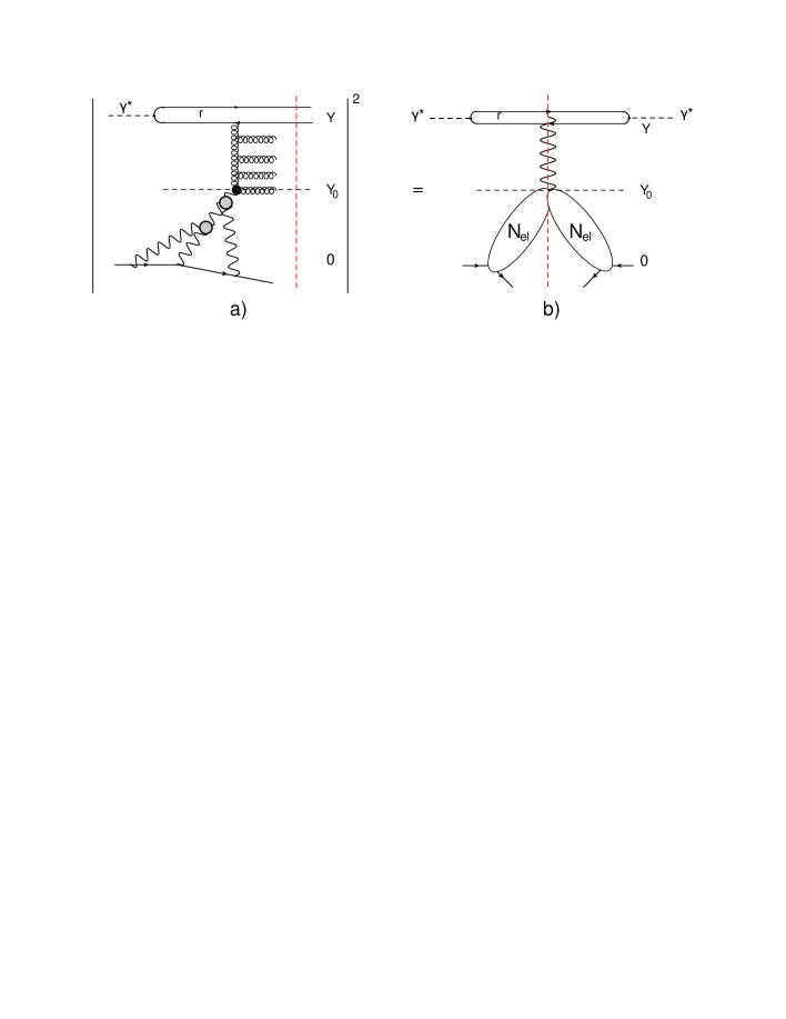
Figure 1: The graphic representation of the processes of diffraction production in the region of high mass. The wavy lines denote the BFKL Pomerons. $Y=\ln\left(1/x_{Bj}\right),Y_{0}=\ln\left(1/x_{I\!\!P}\right)$ and $\beta=Q^{2}/\left(Q^{2}+M^{2}_{X}\right)$, $x_{I\!\!P}=\left(Q^{2}+M^{2}_{X}\right)/s,x_{bj}=Q^{2}/s$ where $Q$ is the photon virtuality, $s$ the squared of energy and $M_{X}$ is the produced mass.

For $N^{D}$ the evolution equation has been derived in Ref.KOLE in the leading log(1/x) approximation (LLA) of perturbative QCD(see Ref.KOLEB for detail and general description of the LLA). Hence, we hope to describe the experimental data only in the kinematic region where both $\beta$ and $x_{I\!\!P}$ are very small ($Y-Y_{0}\,=\,\ln(1/\beta)\,\gg\,1$ and $Y_{0}=\ln(1/x_{{I\!\!P}})\,\gg\,1$ are large).

The equation as has been shown in Ref.KOLE , can be written in two forms. First, it turns out that for the new function

$${\cal N}\left(Y,Y_{0};r_{\perp},b\right)\,\,\equiv\,\,2N_{\rm el}\left(Y;r_{\perp},b\right)\,\,-\,\,N^{D}(r_{\perp},x,x_{0};b)$$ (3)

the equation has the same form as Balitsky-Kovchegov equation BK : viz.

$$\displaystyle{\frac{\partial{\cal N}\left(Y,Y_{0};\boldsymbol{x}_{01},\boldsymbol{b}\right)}{\partial Y}}\, = \,\displaystyle{\bar{\alpha}_{S}\int\frac{d^{2}{\mathbf{x_{2}}}}{2\pi}\frac{{\mathbf{x^{2}_{01}}}}{{\mathbf{x^{2}_{02}}}\,{\mathbf{x^{2}_{12}}}}\Bigg{\{}{\cal N}\left(Y,Y_{0};\boldsymbol{x}_{02},\boldsymbol{b}-\frac{1}{2}\boldsymbol{x}_{12}\right)+{\cal N}\left(Y,Y_{0};\boldsymbol{x}_{12},\boldsymbol{b}-\frac{1}{2}\boldsymbol{x}_{02}\right)\,-\,{\cal N}\left(Y,Y_{0};\boldsymbol{x}_{01},\boldsymbol{b}\right)}\,$$ (4)

$$- \,\displaystyle{{\cal N}\left(Y,Y_{0};\boldsymbol{x}_{02},\boldsymbol{b}-\frac{1}{2}\boldsymbol{x}_{12}\right){\cal N}\left(Y,Y_{0};\boldsymbol{x}_{12},\boldsymbol{b}-\frac{1}{2}\boldsymbol{x}_{02}\right)\Bigg{\}}}$$

with $\bar{\alpha}_{S}\,=\,N_{c}\alpha_{S}/\pi$ where $\alpha_{S}$ is QCD coupling and $N_{c}$ is the number of colours.

Note, that $\boldsymbol{r}=\boldsymbol{x}_{01}$, and the kernel of the equation describes the decay of a dipole to two dipoles: $\boldsymbol{x}_{01}\,\to\,\boldsymbol{x}_{02}\,+\,\boldsymbol{x}_{12}$. The initial condition for Eq. (4) has the following form:

$${\cal N}\left(Y=Y_{0},Y_{0};\boldsymbol{x}_{01},\boldsymbol{b}\right)\,\,=\,\,2\,N_{\rm el}\left(Y=Y_{0};\boldsymbol{x}_{01},\boldsymbol{b}\right)\,-\,N^{2}_{\rm el}\left(Y=Y_{0};\boldsymbol{x}_{01},\boldsymbol{b}\right)$$ (5)

Re-writing Eq. (4) as the equation for $N^{D}$ we obtain the second form of the set of the equations:

$$\frac{\partial N^{D}\left(Y,Y_{0};\boldsymbol{x}_{01},\boldsymbol{b}\right)}{\partial Y}\,=$$ (6)

$$\,\,\bar{\alpha}_{S}\int\,\frac{d^{2}\boldsymbol{x}_{2}}{2\pi}\frac{{\mathbf{x^{2}_{01}}}}{{\mathbf{x^{2}_{02}}}\,{\mathbf{x^{2}_{12}}}}\Bigg{\{}\,N^{D}\left(Y,Y_{0};\boldsymbol{x}_{02},\boldsymbol{b}-\frac{1}{2}\boldsymbol{x}_{12}\right)+N^{D}\left(Y,Y_{0};\boldsymbol{x}_{12},\boldsymbol{b}-\frac{1}{2}\boldsymbol{x}_{02}\right)\,-\,N^{D}\left(Y,Y_{0};\boldsymbol{x}_{01},\boldsymbol{b}\right)$$

$$+\,\,N^{D}(Y,Y_{0};\boldsymbol{x}_{02},\boldsymbol{b}-\frac{1}{2}\boldsymbol{x}_{12})N^{D}(Y,Y_{0};\boldsymbol{x}_{12},\boldsymbol{b}-\frac{1}{2}\boldsymbol{x}_{02})-2\,N^{D}(Y,Y_{0};\boldsymbol{x}_{02},\boldsymbol{b}-\frac{1}{2}\boldsymbol{x}_{12})N_{\rm el}(Y;\boldsymbol{x}_{12},\boldsymbol{b}-\frac{1}{2}\boldsymbol{x}_{02})$$

$$\,\,-2\,N^{D}(Y,Y_{0};\boldsymbol{x}_{12},\boldsymbol{b}-\frac{1}{2}\boldsymbol{x}_{02})N_{\rm el}(Y;\boldsymbol{x}_{02},\boldsymbol{b}-\frac{1}{2}\boldsymbol{x}_{12}\,+2\,N_{\rm el}(Y;\boldsymbol{x}_{02},\boldsymbol{b}-\frac{1}{2}\boldsymbol{x}_{12})N_{\rm el}(Y;\boldsymbol{x}_{12},\boldsymbol{b}-\frac{1}{2}\boldsymbol{x}_{02})]\,\Bigg{\}}.$$

The initial conditions are

$$N^{D}\left(Y=Y_{0},Y_{0};\boldsymbol{x}_{01},\boldsymbol{b}\right)\,\,=\,\,N^{2}_{\rm el}(Y_{0};\boldsymbol{x}_{01},\boldsymbol{b})$$ (7)

Eq. (7) accounts for the production of quark-antiquark pair integrated over its mass.

A general feature, is that the amplitude with fixed rapidity gap can be calculate as follows

$$n^{D}\left(Y,\mbox{ rapidity gap}=Y_{0};\boldsymbol{x}_{01},\boldsymbol{b}\right)\,=\,-\frac{\partial N^{D}\left(Y,Y_{0};\boldsymbol{x}_{01},\boldsymbol{b}\right)}{\partial Y_{0}}\,=\,\frac{\partial{\cal N}\left(Y,Y_{0};\boldsymbol{x}_{01},\boldsymbol{b}\right)}{\partial Y_{0}}\,$$ (8)

It should be noted that the initial condition for $n^{D}\left(Y,\delta Y=Y-Y_{0};\boldsymbol{x}_{01},\boldsymbol{b}\right)\,=\,\,N^{2}_{\rm el}(Y_{0};\boldsymbol{x}_{01},\boldsymbol{b})\,\delta\left(Y-Y_{0}\right)$. The appearance of $\delta$-function is the artifact of the LLA, in which we only sum contributions with large $\delta Y$. However, it has been shown GOLEDD ; MAR ; MUSCH that more careful estimates of the $q\bar{q}$ production leads to smearing of the $\delta$ function and, in the first approximation, the contribution of this production to $n^{D}$ can be written as

$$n^{D}\left(Y,\delta Y=Y-Y_{0};\boldsymbol{x}_{01},\boldsymbol{b}\right)\,\,=\,\,N^{2}_{\rm el}(Y_{0};\boldsymbol{x}_{01},\boldsymbol{b})\,e^{-\delta Y}$$ (9)

Eq. (9) shows that the production of $q\bar{q}$ pairs decreases as $d\sigma/dM^{2}_{X}\,\propto\,1/M^{4}_{x}$, which corresponds to the high energy behaviour of the amplitude due to $q\bar{q}$ exchange (see for example Ref.KOLEB , section 3.2).

III Double log approximation for the produced gluons for $\tau_{0}\,=\,r^{2}\,Q^{2}_{s}\left(Y_{0},b\right)\,<\,1$

In this section we consider the kinematic region in which $N_{\rm el}\left(Y_{0};\boldsymbol{x}_{01},\boldsymbol{b}\right)$ is in the vicinitity of the saturation scale $Q_{s}\left(Y_{0},b\right)$, but at $x^{2}_{01}\,Q^{2}_{s}\left(Y_{0},b\right)\,<\,1$. As it was found in Ref. IIML ; MUT we have geometric scaling behaviour in this region, and the amplitude behaves as

$${N_{\rm el}\left(Y_{0};\boldsymbol{x}_{01},\boldsymbol{b}\right)\,\,=\,\,{\rm c}\,\left(x^{2}_{10}\,Q^{2}_{s}\left(Y_{0},b\right)\right)^{1-\gamma_{cr}}}\,\,<\,\,1$$ (10)

in the leading order approximation of perturbative QCD (LOA) with $\gamma_{cr}=0.37$.

Considering Eq. (10), one can see that in this kinematic region we can, in general, neglect two terms in Eq. (6): the term which is proportional to $\left(N^{D}\right)^{2}$ at $Y-Y_{0}\ll Y_{0}$, since it is of the order of $N^{4}_{\rm el}$, and the term which is proportional to $N^{D}N_{\rm el}\propto N^{3}_{\rm el}$, while we have to keep all other terms.

Therefore, the equation takes the form:

$$\frac{\partial N^{D}\left(Y,Y_{0};\boldsymbol{x}_{01},\boldsymbol{b}\right)}{\partial Y}\,=$$ (11)

$$\,\bar{\alpha}_{S}\int\,\frac{d^{2}\boldsymbol{x}_{2}}{2\pi}\frac{{\mathbf{x^{2}_{01}}}}{{\mathbf{x^{2}_{02}}}\,{\mathbf{x^{2}_{12}}}}\Bigg{\{}\,N^{D}\left(Y,Y_{0};\boldsymbol{x}_{02},\boldsymbol{b}-\frac{1}{2}\boldsymbol{x}_{12}\right)+N^{D}\left(Y,Y_{0};\boldsymbol{x}_{12},\boldsymbol{b}-\frac{1}{2}\boldsymbol{x}_{02}\right)\,-\,N^{D}\left(Y,Y_{0};\boldsymbol{x}_{01},\boldsymbol{b}\right)$$

$$~{}~{}~{}~{}~{}~{}~{}~{}~{}~{}~{}~{}~{}~{}~{}~{}~{}~{}~{}~{}~{}~{}~{}~{}~{}~{}~{}~{}~{}~{}+2\,N_{\rm el}(Y;\boldsymbol{x}_{02},\boldsymbol{b}-\frac{1}{2}\boldsymbol{x}_{12})N_{\rm el}(Y;\boldsymbol{x}_{12},\boldsymbol{b}-\frac{1}{2}\boldsymbol{x}_{02})]\,\Bigg{\}}.$$

In this equation we take into account the corrections of the order $N^{2}_{el}$, but neglected the terms of the order of $N^{3}_{el}$ and $N^{4}_{el}$, assuming they are small. We believe that this equation will allow us to take into account the correction for $N_{el}\approx 0.4-0.5$.

Taking derivatives with respect to $Y_{0}$, we re-write Eq. (11) for the amplitude $n^{D}\left(Y,Y_{0},\boldsymbol{x}_{01},\boldsymbol{b}\right)$ that has been introduced in Eq. (8). It has the form of the linear equation:

$$\frac{\partial n^{D}\left(Y,Y_{0};\boldsymbol{x}_{01},\boldsymbol{b}\right)}{\partial Y}\,=$$ (12)

$$\,\,\bar{\alpha}_{S}\int\,\frac{d^{2}\boldsymbol{x}_{2}}{2\pi}\frac{{\mathbf{x^{2}_{01}}}}{{\mathbf{x^{2}_{02}}}\,{\mathbf{x^{2}_{12}}}}\Bigg{\{}\,n^{D}\left(Y,Y_{0};\boldsymbol{x}_{02},\boldsymbol{b}-\frac{1}{2}\boldsymbol{x}_{12}\right)+n^{D}\left(Y,Y_{0};\boldsymbol{x}_{12},\boldsymbol{b}-\frac{1}{2}\boldsymbol{x}_{02}\right)\,-\,n^{D}\left(Y,Y_{0};\boldsymbol{x}_{01},\boldsymbol{b}\right)\Bigg{\}}$$

The initial condition for this equation sshould be taken from Eq. (9) and it has the form:

$${n^{D}\left(Y_{0},Y_{0};\boldsymbol{x}_{01},\boldsymbol{b}\right)\,\,=\,\,N^{2}_{\rm el}\left(Y_{0};\boldsymbol{x}_{01},\boldsymbol{b}\right)}$$ (13)

The elastic amplitude is:

$$N_{\rm el}(Y;x_{10},b)\,\,=\,\,{\rm c}\left(x^{2}_{10}\,Q^{2}_{s}\left(Y,b\right)\right)^{\bar{\gamma}}\,\,\equiv\,\,{\rm c}\,\,e^{\bar{\gamma}\left(\bar{\alpha}_{S}\kappa\left(Y-Y_{0}\right)\,-\,\xi\right)}$$ (14)

where $\bar{\gamma}=1-\gamma_{cr}$ and $\xi\,\equiv\,\ln\left(1/\left(x^{2}_{10}\,Q^{2}_{s}\left(Y_{0},b\right)\right)\right)$. All other parameters of Eq. (14) will be defined in Eq. (19) below.

Taking the double Mellin transform,

$${n^{D}\left(Y,Y_{0},\xi,b\right)\,\,=\,\,\,\int_{C_{1}}\frac{d\gamma d\omega}{(2\pi i)^{2}}\,\phi(\omega,\gamma)\,e^{\bar{\alpha}_{S}\,\omega\,\left(Y-Y_{0}\right)\,\,+\,\,\left(\gamma-1\right)\xi}}$$ (15)

we obtain the solution to the equation of Eq. (12) in the following form:

$${n^{D}\left(Y,Y_{0},\xi,b\right)\,\,=\,\,\,\int_{C_{1}}\frac{d\gamma d\omega}{(2\pi i)^{2}}\,\frac{\phi_{in}\left(\gamma,Y_{0}\right)}{\omega-\chi\left(\gamma\right)}\,e^{\bar{\alpha}_{S}\,\omega\left(Y-Y_{0}\right)\,\,+\,\,\left(\gamma-1\right)\xi}}$$ (16)

where $\phi_{in}$ has to be determined from the initial condition of Eq. (24), and it has the form

$$\phi_{in}\left(\gamma,Y_{0}\right)\,\,=\,\,\,\frac{c^{2}}{\gamma-\tilde{\gamma}}$$ (17)

where $\bar{\gamma}\,=\,\,1-\gamma_{cr}$. In this paper we will use the value of $\gamma_{cr}$ which comes from the leading order estimates: $\gamma_{cr}\,\approx\,\,0.37$ which gives $\bar{\gamma}\,=\,\,1-\gamma_{cr}=0.63$ ,$\tilde{\gamma}=-1+2\gamma_{cr}=-0.26$.

Therefore, the solutionhas the form (see Fig. 1 for notations):

$${n^{D}\left(Y,Y_{0},\xi,b\right)\,\,=\,\,{\rm c}^{2}\int_{C_{1}}\frac{d\gamma}{2\pi i}\,\frac{1}{\gamma-\tilde{\gamma}}\,e^{\bar{\alpha}_{S}\,\chi\left(\gamma\right)\left(Y-Y_{0}\right)\,\,+\,\,\left(\gamma-1\right)\xi}}$$ (18)

with $\chi\left(\gamma\right)$ and $\kappa$ are equal to

$$\kappa\,\,=\,\,\frac{\chi\left(1-\gamma_{cr}\right)}{1-\gamma_{cr}};\,\,\,\,\chi\left(\gamma\right)\,=\,2\psi\left(1\right)-\psi\left(\gamma\right)-\psi\left(1-\gamma\right);$$ (19)

where $\psi(x)=d\ln\Gamma(x)/dx$ and $\Gamma$ is the Euler gamma function RY .The choice of the contour of integration over $\gamma$ (see Fig. 2) is standard for the solution of the BFKL Pomeron, and correctly reproduces the calculation of the gluon emission in perturbative QCD.

The contour of integration ($C_{1}$) is shown in Fig. 2. Recalling that $x^{2}_{01}\,Q^{2}_{s}\left(Y_{0},b\right)\,<\,1$ and $\xi>0$, we can safely move this contour, and for large values of $\delta Y=Y-Y_{0}$ and $\xi$, we can take the integral using the method of steepest decent. For $\alpha_{S}\delta Y\,\gg\,\xi$ we evaluate the integral by this method, integrating along the contour $C_{2}$ which crosses the real axis at $\gamma$ close to $\frac{1}{2}$. Here, we develop the double log(1/x) approach in which we replace the kernel of Eq. (19) by the $\chi\left(\gamma\right)\,=\,1/\gamma$. At $\xi\,\gg\,\bar{\alpha}_{S}\,\delta Y$, we can integrate by the method of steepest descend, but moving contour $C_{2}$ closer to $y$-axis in Fig. 2. For $\delta Y=0$ we can close the counter over pole $\gamma=\bar{\gamma}$. However, for $\delta Y\sim 1$ we cannot use the same method, since at $\gamma=0$ we have singularities in the kernel $\chi(\gamma)$.

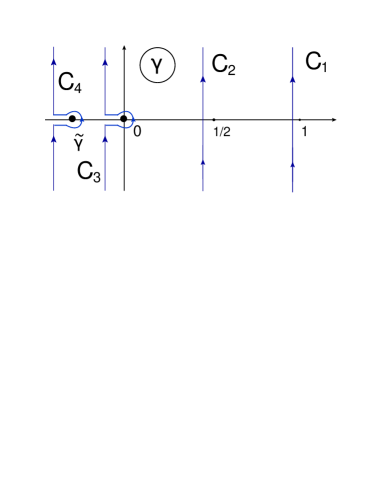
Figure 2: The contours of integration over $\gamma$

For developing the DLA , let us analyze the solution iterating the equation keeping $\bar{\alpha}_{S}\,\delta\,Y\,\,<\,1$. To obtain the solution as a sum of $\left(\delta Y\right)^{n}$ contributions we need to expand

$$e^{\bar{\alpha}_{S}\chi\left(\gamma\right)\left(Y-Y_{0}\right)}\,\,=\,\,\sum^{\infty}_{n=0}\,\frac{\left(\bar{\alpha}_{S}\chi(\gamma)\,\delta Y\right)^{n}}{n!}\,\,\xrightarrow{~{}~{}\gamma\to 0~{}~{}~{}}\,\,\sum^{\infty}_{n=0}\,\frac{1}{n!}\left(\frac{\bar{\alpha}_{S}\,\delta Y}{\gamma}\right)^{n}$$ (20)

For each term of this series, we need to plug in our solution, and integrate over $\gamma$. This integral takes the following form for the third term in Eq. (18) for $n\,\geq\,1$:

$$\oint_{C_{3}}\,d\gamma\,\left(\frac{\bar{\alpha}_{S}\,\delta Y}{\gamma}\right)^{n}\frac{e^{\left(\gamma-1\right)\xi}}{\gamma-\tilde{\gamma}}\,\,=\,\,\left(\bar{\alpha}_{S}\,\delta Y\right)^{n}\Bigg{\{}\frac{1}{\tilde{\gamma}}\frac{1}{(n-1)!}\left(\frac{e^{\left(\gamma-1\right)\xi}}{\gamma-\tilde{\gamma}}\right)^{(n)}_{\gamma,\gamma\to 0}\,+\,\frac{1}{\tilde{\gamma}^{n}}\,e^{\left(\tilde{\gamma}-1\right)\xi}\Bigg{\}}$$ (21)

For $n=0$, we only have the contribution of the second term in Eq. (21).

In Eq. (20) we evaluated the integral, closing the contour over the singularities of the BFKL kernel, which is the pole at $\gamma=0$, and over the pole $\gamma=\tilde{\gamma}$. The BFKL kernel also has poles at $\gamma\,=\,-n,\,n=1,2,3\dots$, but their contributions are exponentially suppressed with $\xi$ leading to the next twists contributions. Eq. (21) can be re-written as follows

$$\oint_{C_{3}}\,d\gamma\,\left(\frac{\bar{\alpha}_{S}\,\delta Y}{\gamma}\right)^{n}\frac{e^{\left(\gamma-1\right)\xi}}{\gamma-\tilde{\gamma}}\,\,=\,\,\left(\frac{\bar{\alpha}_{S}\,\delta Y}{\tilde{\gamma}}\right)^{n}\,e^{-\xi}\,\Bigg{\{}\frac{1}{\tilde{\gamma}}\frac{1}{(n-1)!}\,\sum_{k=0}^{n-1}\frac{\left(\tilde{\gamma}\,\xi\right)^{k}}{k!}\,\,+\,\,e^{\tilde{\gamma}\,\xi}\Bigg{\}}$$ (22)

The last term in Eq. (22) is the contribution at the pole $\gamma=\tilde{\gamma}$, while the first term is the sum of logs term giving the leading twist perturbative series.

Bearing this in mind we can re-write Eq. (18) in the following form

$$n^{D}\left(Y,Y_{0},\xi,b\right)\,\,=\\ \,\,{\rm c}^{2}\,\Bigg{\{}\int_{C_{1}-C_{4}}\frac{d\gamma}{2\pi i}\,\frac{1}{\gamma-\tilde{\gamma}}\,e^{\bar{\alpha}_{S}\,\chi\left(\gamma\right)\left(Y-Y_{0}\right)\,\,+\,\,\left(\gamma-1\right)\xi}\,\,+\,\,e^{\left(\tilde{\gamma}-1\right)\xi}\,e^{\bar{\alpha}_{S}\chi\left(\tilde{\gamma}\right)\,\left(Y-Y_{0}\right)}\Bigg{\}}$$ (23)

The first term in Eq. (23) is the difference between two integrals with contour $C_{1}$ and $C_{4}$, while the last term is the result of integrating over $\gamma$, with the contour $C_{4}$. The advantage of this form for the equation, is that it satisfies the initial condition, since the first term is equal to zero at $\delta Y=0$, and the first term generates all perturbative logs with respect to the dipole sizes.

In the situation when $\bar{\alpha}_{S}\,\delta Y\,\xi\,\geq\,1$ while $\bar{\alpha}_{S}\,\ll\,1$, the first term reduces to the double log approximation generating the contribution

$$n^{D}_{\rm 1-st\,term\,of\,{Eq.~{}(\ref{CR2})}}\left(Y,Y_{0},r\right)\,\,=\,\,{\rm c}^{2}\,\frac{\bar{\alpha}_{S}\delta Y}{|\bar{\gamma}|}\,e^{-\xi}\,\sum^{\infty}_{n=1}\frac{1}{n!(n-1)!}\left(\bar{\alpha}_{S}\delta Y\xi\right)^{n-1}\,=\,{\rm c}^{2}\,\frac{1}{|\bar{\gamma}|}\,\sqrt{\frac{\bar{\alpha}_{S}\delta Y}{\xi}}\,e^{-\xi}I_{1}\left(2\sqrt{\bar{\alpha}_{S}\delta Y\,\xi}\right)$$ (24)

which stems from the term with $\xi^{n-1}$ in Eq. (22).

Finally the double log contribution takes the form:

$$n^{D}\left(Y,Y_{0},\xi\right)\,\, = \,\,{\rm c}^{2}\Bigg{\{}\frac{\bar{\alpha}_{S}}{|\tilde{\gamma}|}\sqrt{\frac{\bar{\alpha}_{S}\delta Y}{\xi}}\,e^{-\xi}I_{1}\left(2\sqrt{\bar{\alpha}_{S}\delta Y\,\xi}\right)\,+\,\,e^{\left(\tilde{\gamma}-1\right)\xi}\,e^{-\frac{\bar{\alpha}_{S}}{\tilde{\gamma}}\,\left(Y-Y_{0}\right)}\Bigg{\}}$$ (25a)

$$= {\rm c}^{2}\frac{\bar{\alpha}_{S}}{|\tilde{\gamma}|}\sqrt{\frac{\bar{\alpha}_{S}\delta Y}{\xi}}\,e^{-\xi}I_{1}\left(2\sqrt{\bar{\alpha}_{S}\delta Y\,\xi}\right)\,\,+\,\,N^{2}_{el}\left(Y;\xi\right)\,e^{-\lambda_{1}\,\delta Y}$$ (25b)

In the leading order estimates the value of $\lambda_{1}=\bar{\alpha}_{S}/\tilde{\gamma}+2\,\bar{\alpha}_{S}/\gamma_{cr}$. However, this term describes the quark-antiquark production whose $\delta Y$ behaviour is given by Eq. (9). Based on this equation and, having in mind that the next to leading order corrections are large, we consider $\lambda_{1}$ as a free parameter in the description of the experimental data. We expect $\lambda_{1}\approx 1$ from Eq. (9), but we will discuss this term below in more detail.

In appendix A we remove the assumption that $\bar{\alpha}_{S}\,\delta Y\,\xi\gg\,1$.

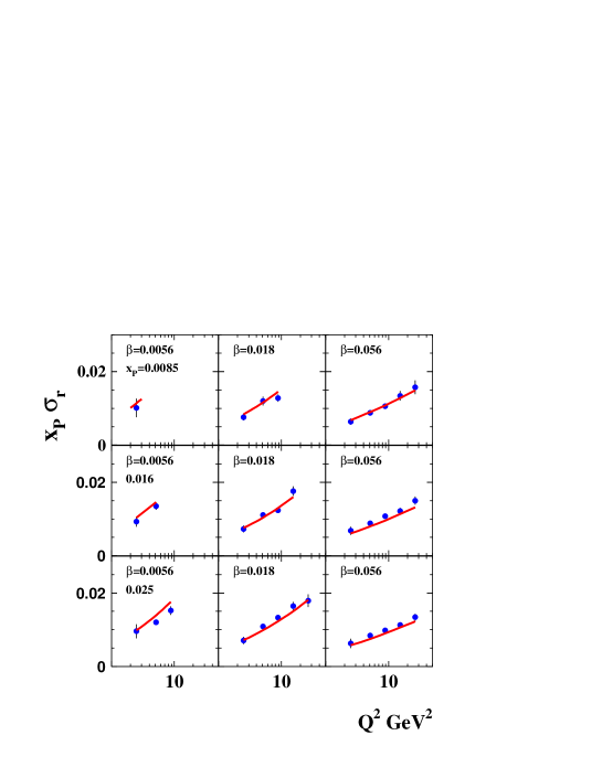
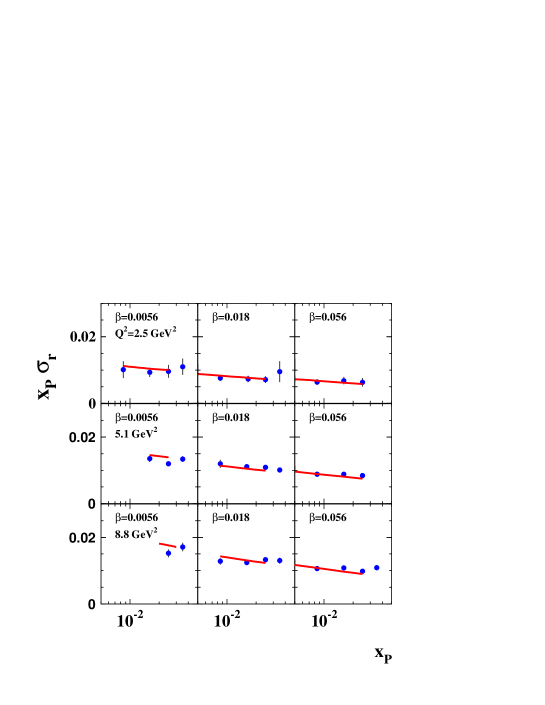
Fig. 3-a	Fig. 3-b

Figure 3: $\sigma^{\rm diff}\left(Y,Y_{0},Q^{2}\right)=x_{I\!\!P}\,\sigma_{r}$ versus $Q^{2}$ at fixed $\beta$ and $x_{I\!\!P}$ (Fig. 3-a) and versus $x_{I\!\!P}$ at fixed $\beta$ and $Q^{2}$ (Fig. 3-b). The data are taken from Ref. HERADATA .

Using Eq. (25b) we attempted to describe the combined set of the inclusive diffractive cross sections measured by H1 and ZEUS collaboration at HERA HERADATA . The measured cross sections were expressed in terms of reduced cross sections, $\sigma_{r}^{D(4)}$, which is related to the measured $ep$ cross section by

$$\frac{{\rm d}\sigma^{ep\rightarrow eXp}}{{\rm d}\beta{\rm d}Q^{2}{\rm d}\boldsymbol{x}_{I\!\!P}{\rm d}t}=\frac{4\pi\alpha^{2}}{\beta Q^{4}}\ \ \left[1-y+\frac{y^{2}}{2}\right]\ \ \sigma_{r}^{D(4)}(\beta,Q^{2},x_{I\!\!P},t)\ .$$ (26)

In the paper, the table of $x_{I\!\!P}\sigma_{r}^{D(3)}(\beta,Q^{2},x_{I\!\!P})=x_{I\!\!P}\int dt\,\,\sigma_{r}^{D(4)}(\beta,Q^{2},x_{I\!\!P},t)$ are presented at different values of $Q,\beta$ and $x_{I\!\!P}$. This cross section is equal to $\,\frac{Q^{2}}{4\pi^{2}}\,\sigma^{\rm diff}\left(Y,Y_{0},Q^{2}\right)$ where $\sigma^{\rm diff}\left(Y,Y_{0},Q^{2}\right)$ is given by Eq. (1). In the experimental data from Ref. HERADATA the integral in $t$ was performed in the region $0.09\,\leq\,t\,\leq 0.55\,GeV^{2}$, while our formulae are derived for the integration in $t$ from 0 to $\infty$. Assuming that the $b$-dependence of the saturation scale $Q_{s}\left(Y_{0},b\right)$ is the same as was suggested in Ref. CLP we estimate that the experimentally measured region in $t$ leads to factor 0.52 in $x_{I\!\!P}\sigma_{r}^{D(3)}(\beta,Q^{2},x_{I\!\!P})$.

For the fit 61 experimental points were selected which satisfy the following criteria: $Q^{2}\,\leq\,26.5\,GeV^{2}$, $\beta\,\leq\,0.18$ and $x_{I\!\!P}\,\leq\,0.025$. The region of $Q^{2}$ and $x_{I\!\!P}$ was chosen from the description of the HERA data for inclusive DISCLP , as the specification of the region of small $x_{I\!\!P}$, where the saturation model is able to fit the experimental data. The maximal value of $\beta$ can be considered as outcome of the fit. For larger $\beta$, our approach cannot describe the data. For this sample we obtain the fit with $\bar{\alpha}_{S}=0.119$ and $\lambda_{1}=0.6$ for the massless light quarks and for $m_{c}=1.4\,GeV$, where $m_{c}$ is the mass of $c$-quark. The value of $\chi^{2}$ is equal 62 leading to $\chi^{2}/{\rm d.o.f.}\,=1.02$. In Fig. 3 we show examples of the comparison of Eq. (25b) with the experimental data As expected $\lambda_{1}$ turns out to be close to 1. $N_{el}$ has been taken from Ref.CLP , where the HERA data on $F_{2}$, have been described in the CGC/saturation approach. It is instructive to note, that the value of parameter $c$, which is needed to fit the data, turns out to be about $0.3-0.4$. We believe, we can apply our approximation for such values of $c$. Comparing with the description of the same data in our previous paperCLMP , one can see that we obtain a much better agreement.

In Fig. 4 we show the average multiplicity of the emitted gluons $n=\sqrt{\bar{\alpha}_{S}\,\delta Y\,\xi}I_{0}\left(2\sqrt{\bar{\alpha}_{S}\,\delta Y\,\xi}\right)\Big{/}I_{1}\left(2\sqrt{\bar{\alpha}_{S}\,\delta Y\,\xi}\right)$. One can see, that we cannot restrict ourselves by calculating only one emitted gluon, as it has been discussed in Refs.GBKW ; GOLEDD ; SATMOD0 ; KOML ; MUSCH ; MASC ; MAR ; KLMV . On the other hand, the density is not large to use the CGC/saturation approach for this system of gluons. As we have discussed we developed the DLA, assuming that $\bar{\alpha}_{S}\,\ll\,1,\bar{\alpha}_{S}\,\xi\ll\,1,\,\bar{\alpha}_{S}\,\delta Y\,\ll\,1$ but $\bar{\alpha}_{S}\,\delta Y\,\xi\,\sim\,1$. We checked that describing the experimental data we have $\bar{\alpha}_{S}\,\xi\leq 0.35$ and $\bar{\alpha}_{S}\delta Y\,\leq\,0.6$ while $0.3\,<\,\bar{\alpha}_{S}\delta Y\xi\,<\,2$. Based on this estimates we believe that DLA can produce a good first approximation for understanding the structure of the produced gluons. On the other hand, these estimates show that we need to go beyond the DLA. The first corrections of this type we discuss in the appendix. Using Eq. (77) we tried to describe the data and obtain a good fit with $\chi^{2}=66$ for 61 experimental points. The values of parameters $\lambda_{1}=0.608$ and $\bar{\alpha}_{S}=0.149$ turns out to be close to the previous fit, showing that the corrections work in the right direction increasing the value of $\bar{\alpha}_{S}$. We firmly believe that the small values of the fitted $\bar{\alpha}_{S}$ stems from the higher order corrections, which should be taken into account.

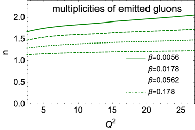
Figure 4: The average multiplicities of the emitted gluon at different values of $\beta$ as function of $Q^{2}$ using the parameters of the fit.

As has been mentioned we integrated in Eq. (1) only over kinematic region where $\tau_{0}\,=\,r^{2}\,Q^{2}_{s}\left(Y_{0},b\right)\,\leq\,1$. However, the region of $\tau_{0}\,\geq 1$ does not give a negligible contribution. We checked this, integrating the second term in Eq. (25b) over all $r$. We got reasonable description of the data reaching $\chi^{2}=100$ for 61 points but the values of parameters $\bar{\alpha}_{S}$ and $\lambda_{1}$ turn out to be quite different for this fit : $\bar{\alpha}_{S}=0.128$ and $\lambda_{1}=0.95$. This shows that we need to consider the kinematic region $\tau_{0}\,\leq\,1$. We do this in the next section.

IV Double log approximation for the produced gluons for $\tau_{0}\,=\,r^{2}\,Q^{2}_{s}\left(Y_{0},b\right)\,\leq\,1$

In this section we will consider Eq. (6), assuming that the elastic amplitude $N_{el}$ is in the saturation region with $\tau_{0}\,\approx\,1$. We consider that in this kinematic region $N_{el}\left(\tau_{0}=1\right)$ is not a small value, but is of the order of 1, and, therefore, we cannot use the small sizes of $N^{3}_{el}$ and $N^{4}_{el}$ as we did deriving Eq. (12).

We start with specification of Eq. (9) for the quark-antiquark production. This process has been discussed in Refs.GBKW ; GOLEDD ; SATMOD0 ; KOML ; MUSCH ; MASC ; MAR ; KLMV and we briefly review the results for the completeness of the presentation.

IV.1 $q\bar{q}$ production.

The total cross section of the quark-antiquark pair production is determined by $N^{2}_{\rm el}\left(r_{\perp},Y;\boldsymbol{b}\right)$ and it can be found from Eq. (1) with

$$\sigma_{\rm dipole}^{diff}(r_{\perp},Y)\,\,=\,\,\int d^{2}b\,N^{2}_{\rm el}\left(r_{\perp},Y;\boldsymbol{b}\right)$$ (27)

We need to re-write Eq. (1) in the following form to obtain the contribution of the $q\bar{q}$ production to the cross section with fixed produced mass $M_{X}$:

$$\sigma^{\rm diff}(Y,Q^{2})\,\,=\,\,\int dM^{2}_{X}\,\int\frac{d^{2}k_{T}}{(2\pi)^{2}}\,\delta\left(M^{2}_{X}\,-\,\frac{k^{2}_{T}}{z(1-z)}\right)\Bigg{(}\int d^{2}r_{\perp}\Psi^{\gamma^{*}}\left(Q;r_{\perp},z\right)N_{\rm el}\left(r_{\perp},Y;\boldsymbol{b}\right)\Psi^{q\bar{q}}\left(\boldsymbol{k}_{T};\boldsymbol{r}_{\perp}\right)\Bigg{)}^{2}$$ (28)

From Eq. (28) one can see that

$$\left(M^{2}_{X}+Q^{2}\right)\frac{d\sigma^{\rm diff}(Y,Y_{M}\,=\,\delta Y;Q^{2})}{dM^{2}_{X}}\,\,=\,\,x_{{I\!\!P}}\frac{d\sigma^{\rm diff}(Y,Y_{M}\,=\,\delta Y;Q^{2})}{dx_{{I\!\!P}}}\,=\,\frac{d\sigma^{\rm diff}(Y,Y_{M}\,=\,\delta Y;Q^{2})}{dY_{0}}\,\,$$

$$=\,\,\left(M^{2}_{X}+Q^{2}\right)\int^{1}_{0}dz\int d^{2}b\int\frac{d^{2}k_{T}}{(2\pi)^{2}}\,\delta\left(M^{2}_{X}\,-\,\frac{k^{2}_{T}}{z(1-z)}\right)\Bigg{(}\int d^{2}r_{\perp}\Psi^{\gamma^{*}}\left(Q;\boldsymbol{r}_{\perp},z\right)N_{\rm el}\left(r_{\perp},Y;\boldsymbol{b}\right)\Psi^{q\bar{q}}\left(\boldsymbol{k}_{T};\boldsymbol{r}_{\perp}\right)\Bigg{)}^{2}$$

$$=\,\,\,\frac{Q^{2}}{\beta}\,\int d^{2}b\int^{1}_{0}\!\!\!\!\!z(1-z)\,dz\Bigg{(}\int d^{2}r_{\perp}\Psi^{\gamma^{*}}\left(Q;\boldsymbol{r}_{\perp},z\right)N_{\rm el}\left(r_{\perp},Y;\boldsymbol{b}\right)\Psi^{q\bar{q}}\left(\boldsymbol{k}_{T};\boldsymbol{r}_{\perp}\right)\Bigg{)}^{2}\Bigg{|}_{k^{2}_{T}=M^{2}_{X}\,z\,(1-z)}$$ (29)

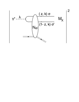
Figure 5: The diffraction production of the quark-antiquark pair with mass $M_{X}$. $\lambda,\sigma$ and $\sigma^{\prime}$ are photon, quark and antiquark helicities.

The wave functions of photon are known (see Ref. KOLEB Eqs.4.18 and 4.20) and have the following for

$\Psi^{q\bar{q}}\left(\boldsymbol{k}_{T};\boldsymbol{r}_{\perp}\right)$ are the plane waves. Plugging Eq. (30a) and Eq. (30c) into Eq. (IV.1) we obtain

$$\Psi_{T}\left(Q;r_{\perp},z\right)\, = \,\frac{eZ_{f}}{2\pi}\Bigg{\{}(1-\delta_{\sigma,\sigma})\,\left(1-2\,z\,-\,\sigma\,\lambda\right)\,ia_{f}\frac{\boldsymbol{\epsilon}^{\lambda}_{\perp}\cdot\boldsymbol{r}_{\perp}}{r_{\perp}}K_{1}\left(r_{\perp}\,a_{f}\right)\,+\,\delta_{\sigma\sigma^{\prime}}\frac{m_{f}}{\sqrt{2}}\left(1+\sigma\lambda\right)K_{0}\left(r_{\perp}\,a_{f}\right)\Bigg{\}};$$ (30a)

$$N_{T} = \,\,Q^{2}z(1-z)\,\,+\,\,m^{2}_{f}~{}~{}~{}~{}\mbox{where}~{}~{}m_{f}~{}~{}\mbox{ mass of the quark};$$ (30b)

$$\Psi_{L}\left(Q;r_{\perp},z\right)\, = \,\frac{eZ_{f}}{2\pi}2Qz(1-z)\left(1-\delta_{\sigma,\sigma^{\prime}}\right)K_{0}\left(r_{\perp}\,a_{f}\right)$$ (30c)

Plugging Eq. (30a) and Eq. (30c) into Eq. (IV.1) and taking into account that $\Psi^{q\bar{q}}$ are plane waves we obtain

$$\,\frac{d\sigma^{\rm diff}_{T}(Y,Y_{M}\,=\,\delta Y;Q^{2})}{dY_{0}} = \,\frac{2N_{c}\,\alpha_{\rm e.m.}}{\pi^{2}}\sum Z^{2}_{f}\frac{Q^{2}}{\beta}\int d^{2}b\int^{1}_{z}z(1-z)dz\left(N_{T}F^{2}_{T}\,+\,m^{2}_{f}\,F^{2}_{L}\right);$$ (31a)

$$\,\frac{d\sigma^{\rm diff}_{L}(Y,Y_{M}\,=\,\delta Y;Q^{2})}{dY_{0}} = \,\frac{2N_{c}\,\alpha_{\rm e.m.}}{\pi^{2}}\sum Z^{2}_{f}\frac{4Q^{4}}{\beta}\int d^{2}b\int^{1}_{z}\left(z(1-z)\right)^{3}dz\,F^{2}_{L};$$ (31b)

where $N_{T}=z+(1-z)^{2}$ and

$$F_{T}\, = \,\int\frac{r_{\perp}dr_{\perp}}{2}\,a_{f}\,K_{1}\left(a_{f}\,r_{\perp}\right)\,J_{1}\left(Q\sqrt{z(1-z))}\sqrt{\frac{1-\beta}{\beta}}\,r_{\perp}\right)\,N_{\rm el}\left(Y,r_{\perp};b\right);$$ (32a)

$$F_{L}\, = \,\int\frac{r_{\perp}dr_{\perp}}{2}\,\,K_{0}\left(a_{f}\,r_{\perp}\right)\,J_{0}\left(Q\sqrt{z(1-z))}\sqrt{\frac{1-\beta}{\beta}}\,r_{\perp}\right)\,N_{\rm el}\left(Y,r_{\perp};b\right)$$ (32b)

IV.2 Initial condition for evolution of $n^{D}$

We need to return to Eq. (6) to find the initial condition for the emission of the gluons in $n^{D}$. First, we will make the first iteration of this equation using Eq. (7) as the initial condition. Plugging in the initial condition for $N^{D}$ from Eq. (7) we obtain:

$$\frac{\partial}{\partial\,\delta Y}N^{D}\left(Y,Y_{0};\boldsymbol{x}_{01},\boldsymbol{b}\right)\,\,=\,\,\,\frac{\bar{\alpha}_{S}}{2\,\pi}\,x^{2}_{10}\,\int\,\frac{d^{2}\boldsymbol{x}_{02}}{\boldsymbol{x}^{2}_{02}\,\boldsymbol{x}^{2}_{12}}\Bigg{\{}-\,N^{2}_{\rm el}\left(Y_{0},\boldsymbol{x}_{01},\boldsymbol{b}\right)$$ (33)

$$+\,\,\Bigg{(}\,N_{\rm el}\left(Y_{0},\boldsymbol{x}_{02},\boldsymbol{b}-\frac{1}{2}\boldsymbol{x}_{12}\right)\,+\,N_{\rm el}\left(Y_{0},\boldsymbol{x}_{12},\boldsymbol{b}-\frac{1}{2}\boldsymbol{x}_{02}\right)-\,N_{\rm el}\left(Y_{0},\boldsymbol{x}_{02},\boldsymbol{b}-\frac{1}{2}\boldsymbol{x}_{12}\right)\,N_{\rm el}\left(Y_{0},\boldsymbol{x}_{12},\boldsymbol{b}-\frac{1}{2}\boldsymbol{x}_{02}\right)\Bigg{)}^{2}\Bigg{\}}$$

In Eq. (33) we have two region of integrations $x_{01}\,\gg\boldsymbol{x}_{02}$ (or $x_{01}\,\gg\boldsymbol{x}_{12}$ ) and $x_{20}\,\gg\,x_{10}$, which can lead to large logs and correspond to the singularities of the BFKL kernel. Let us first consider the region $x_{01}\,\gg\boldsymbol{x}_{02}$. In this region Eq. (33) takes the form:

$$\frac{\partial}{\partial\,\delta Y}N^{D}\left(Y,Y_{0};\boldsymbol{x}_{01},\boldsymbol{b}\right)\,\,\equiv\,\,I_{1}\,\,=\,\,\,\frac{1}{2}\,\bar{\alpha}_{S}\,\int^{x^{2}_{01}}\,\frac{d\boldsymbol{x}^{2}_{02}}{\boldsymbol{x}^{2}_{02}}\Bigg{\{}-\,N^{2}_{\rm el}\left(Y_{0};\boldsymbol{x}_{01},\boldsymbol{b}\right)$$ (34)

$$+\,\,\Bigg{(}\,N_{\rm el}\left(Y_{0};\boldsymbol{x}_{02},\boldsymbol{b}-\frac{1}{2}\boldsymbol{x}_{01}\right)\,+\,N_{\rm el}\left(Y_{0};\boldsymbol{x}_{01},\boldsymbol{b}-\frac{1}{2}\boldsymbol{x}_{02}\right)-\,N_{\rm el}\left(Y_{0};\boldsymbol{x}_{02},\boldsymbol{b}-\frac{1}{2}\boldsymbol{x}_{01}\right)\,N_{\rm el}\left(Y_{0};\boldsymbol{x}_{01},\boldsymbol{b}-\frac{1}{2}\boldsymbol{x}_{02}\right)\Bigg{)}^{2}\Bigg{\}}$$

From Eq. (34) we see that the log term which is originated from the gluon reggeization (the first term in the RHS of Eq. (33) and Eq. (34)), cancels with the term $(\dots)^{2}$ and the resulting integral over $x_{02}$ leads to the contribution which is proportional to $N^{2}_{\rm el}\left(Y_{0},\boldsymbol{x}_{01},\boldsymbol{b}\right)\,\sim\,\tau_{0}^{2\bar{\gamma}}$ (see appendix B for more detailed discussion of this contribution). We show below that this contribution is much smaller than the contribution that stem from the region of integration $x_{20}\,\gg\,x_{10}$ which generates $\ln\left(x^{2}_{10}\,Q^{2}_{s}\left(Y_{0},b\right)\right)$. The reason for this is that this term does not generate the log contribution ($\propto\xi^{n}$) and can be neglected in the DLA.

One can see that the the first iteration in this kinematic region is

$$\frac{\partial}{\partial\,\delta Y}\frac{N^{D}\left(Y,Y_{0};\boldsymbol{x}_{01},\boldsymbol{b}\right)}{x^{2}_{10}}\, = \,\frac{\bar{\alpha}_{S}}{2\,\pi}\int_{x_{10}}\,\frac{d^{2}\boldsymbol{x}_{02}}{\boldsymbol{x}^{4}_{20}}\Bigg{(}\,2\,N_{\rm el}\left(Y_{0};\boldsymbol{x}_{02},\boldsymbol{b}-\frac{1}{2}\boldsymbol{x}_{02}\right)\,-\,N^{2}_{\rm el}\left(Y_{0};\boldsymbol{x}_{02},\boldsymbol{b}-\frac{1}{2}\boldsymbol{x}_{02}\right)\Bigg{)}^{2}$$ (35)

The term of Eq. (35) stems from the emission of an extra gluon from quark - antiquark pair, while Eq. (34) describes the contribution of the virtual gluon to the $q\bar{q}$ production. In the general equation (see Eq. (6) ) this term corresponds to the reggeization of gluons.

The first observation is that the integral in the LHS of Eq. (35) is converged since

$$N_{\rm el}\left(Y;\boldsymbol{x}_{02},\boldsymbol{b}-\frac{1}{2}\boldsymbol{x}_{02}\right)\,\,=\,\,\left\{\begin{array}[]{l}\,\,\,\propto\,\,\left(x_{02}^{2}\,Q^{2}_{s}\left(Y_{0},b\right)\right)^{1-\gamma_{cr}}\,\,\,\,\,\mbox{for }\,\,\,x_{02}^{2}\,Q^{2}_{s}\left(Y_{0},b\right)\,\leq\,1\,\,\mbox{with}\,\,\gamma_{cr}=0.37;\\ \\ \,\,\,1\,\,-\,\,{\rm Const}\exp\left(-z^{2}/(2\kappa)\right)\,\,\,\,\,\mbox{for}\,\,\,x_{02}^{2}\,Q^{2}_{s}\left(Y_{0},b\right)\,\geq\,1\,;\end{array}\right.$$ (39)

where $z\,\,=\,\,\ln\left(x_{02}^{2}\,Q^{2}_{s}\left(Y_{0},b\right)\right)$.

Therefore, we can integrate in Eq. (35) from $x_{02}=0$. The RHS of Eq. (35) is $n^{D}\left(Y=Y_{0},Y_{0},x_{01};b\right)$ (see Eq. (8)). Finally, the initial condition for $n^{D}$ takes the form

$$n^{D}\left(Y=Y_{0},Y_{0},x_{01};b\right)\,\, = \,\,\frac{\bar{\alpha}_{S}}{2\,\pi}x^{2}_{01}\,\int_{0}\,\frac{d^{2}\boldsymbol{x}_{02}}{\boldsymbol{x}^{4}_{20}}\Bigg{(}\,2\,N_{\rm el}\left(Y_{0};\boldsymbol{x}_{02},\boldsymbol{b}-\frac{1}{2}\boldsymbol{x}_{02}\right)\,-\,N^{2}_{\rm el}\left(Y_{0};\boldsymbol{x}_{02},\boldsymbol{b}-\frac{1}{2}\boldsymbol{x}_{02}\right)\Bigg{)}^{2}$$ (40)

$$\,\,=\,\, \frac{\bar{\alpha}_{S}}{2\,\pi}\,\,x^{2}_{01}\,\bar{Q}^{2}\left(Y_{0},b\right)$$

with

$$\bar{Q}^{2}\left(Y_{0},b\right)\,\, = \,\,\int\frac{d^{2}\boldsymbol{x}_{02}}{\boldsymbol{x}^{4}_{20}}\Bigg{(}\,2\,N_{\rm el}\left(Y_{0};\boldsymbol{x}_{02},\boldsymbol{b}-\frac{1}{2}\boldsymbol{x}_{02}\right)\,-\,N^{2}_{\rm el}\left(Y_{0};\boldsymbol{x}_{02},\boldsymbol{b}-\frac{1}{2}\boldsymbol{x}_{02}\right)\Bigg{)}^{2}\,\,$$ (41)

$$= \,\,\,\,Q^{2}_{s}\left(Y_{0},b\right)\int\frac{\pi d\tau_{0}}{\tau^{2}_{0}}\Bigg{(}\,2\,N_{\rm el}\left(\tau_{0}\right)\,-\,N^{2}_{\rm el}\left(\tau_{0}\right)\Bigg{)}^{2}\,\,\,=\,\,\varepsilon\,\,Q^{2}_{s}\left(Y_{0},b\right)\,$$

where $\varepsilon$ is a constant. Since the integral over $\tau_{0}$ is convergent, the typical value of $\tau_{0}$ cannot be found analytically and we used our model CLP to estimate it. It turns out that $\varepsilon\,\approx\,\,1.2$.

It should be stressed that this contribution to $n^{D}$ is proportional to $x^{2}_{01}\,Q^{2}_{s}\left(Y_{0},b\right)$ and it is much larger than the contribution of the order of $\tau_{0}^{2\bar{\gamma}}$ that stems from the region $x^{2}_{01}\,\gg\,x^{2}_{02}$.

Finally, collecting all terms for the initial condition of $n^{D}$ we obtain

$$n^{D}\left(Y=Y_{0},Y_{0};x_{01},b\right)\,\,=\,\,\frac{\bar{\alpha}_{S}}{2\,\pi}\,\,x^{2}_{01}\,\bar{Q}^{2}\left(Y_{0},b\right)\,\,\,-\,\,5.62\,\,\bar{\alpha}_{S}N_{\rm el}^{2}(Y_{0};x_{10},b)$$ (42)

where the last term we discuss in the appendix B.

The first term in Eq. (42) was firstly derived in Ref. MAR , considering the extra gluon emission in perturbative QCD. Here, we derived it directly from Eq. (6) and and Eq. (8).

IV.3 DLA

Based on experience of the previous section we do not expect the number of emitted gluons will be large. Hence, we need to solve linear evolution equation (see Eq. (12)), with the initial condition of Eq. (42). This equation in the DLA takes the form

$$\frac{\partial}{\partial\,\delta Y}\Bigg{(}\frac{n^{D}\left(Y,Y_{0};\boldsymbol{x}_{01},\boldsymbol{b}\right)}{x^{2}_{01}}\Bigg{)}\,\,=\,\,\,\,\bar{\alpha}_{S}\,\int_{x^{2}_{01}}\!\!\!\frac{d\boldsymbol{x}^{2}_{02}}{\boldsymbol{x}^{2}_{02}}\,\Bigg{(}\frac{n^{D}\left(Y,Y_{0};\boldsymbol{x}_{02},\boldsymbol{b}\right)}{x^{2}_{02}}\Bigg{)}$$ (43)

Eq. (43) can be solved by the iteration with the answer:

$$n^{D}\left(Y,Y_{0};\boldsymbol{x}_{01},\boldsymbol{b}\right)\,\,=\,\,\frac{\bar{\alpha}_{S}}{2\,\pi}\,\,x^{2}_{01}\,\bar{Q}^{2}\left(Y_{0},b\right)\,\,I_{0}\left(2\sqrt{\bar{\alpha}_{S}\,\delta Y\,\xi}\right)\,\,=\,\,\varepsilon\,\frac{\bar{\alpha}_{S}}{2\,\pi}\,\,x^{2}_{01}\,Q_{s}^{2}\left(Y_{0},b\right)\,\,I_{0}\left(2\sqrt{\bar{\alpha}_{S}\,\delta Y\,\xi}\right)$$ (44)

The cross section has the following form

$$\sigma^{\rm diff}(Y,Y_{0},Q^{2})\,\,\, = \,\,\int\,\,d^{2}r_{\perp}\int\,dz\,\,|\Psi^{\gamma^{*}}(Q^{2};r_{\perp},z)|^{2}\,\int d^{2}b\,n^{D}_{{Eq.~{}(\ref{DLA2})}}\left(Y,Y_{0};\boldsymbol{x}_{01},\boldsymbol{b}\right)\,\,$$ (45)

$$+ \,\,\,\left(1-\,5.62\,\bar{\alpha}_{S}\right)\left(\frac{d\sigma^{\rm diff}_{T}(Y,Y_{M}\,=\,\delta Y;Q^{2})}{dY_{0}}\Bigg{|}_{{Eq.~{}(\ref{XST})}}\,+\,\,\,\frac{d\sigma^{\rm diff}_{L}(Y,Y_{M}\,=\,\delta Y;Q^{2})}{dY_{0}}\Bigg{|}_{{Eq.~{}(\ref{XSL})}}\right)$$

We compare Eq. (45) with the experimental data, choosing 42 experimental points (see Ref.HERADATA ) with $\beta\,\leq\,0.056$. All other kinematic variables were the same, as in section III, in this comparison. We obtain the description with $\chi^{2}=82$ and $\bar{\alpha}_{S}=0.063$. One can see that the value of $\bar{\alpha}_{S}$ turns out to be smaller than in the previous section. This fact can be an indication that the higher order corrections are essential, that we need to take into account the full DGLAP kernel for $\xi$ evolution. The high order correction we leave for the future publications, and consider the full DGLAP approach in the next section.

As far as comparison with the experimental data is concerned, we consider the comparison as a good, especially since we had only one parameter.

IV.4 $n^{D}$ in the vicinity of the saturation scale $Q_{s}\left(Y-Y_{0},b\right)$

Eq. (44) can be re-written at large $\delta Y$ as

$$n^{D}\left(Y,Y_{0};\boldsymbol{x}_{01},\boldsymbol{b}\right)\,\, = \,\varepsilon\,\frac{\bar{\alpha}_{S}}{2\,\pi}\,\,x^{2}_{01}\,Q_{s}^{2}\left(Y_{0},b\right)\,\,I_{0}\left(2\sqrt{\bar{\alpha}_{S}\,\delta Y\,\xi}\right)$$ (46)

$$\xrightarrow{\bar{\alpha}_{S}\,\delta Y\,\xi\,\gg\,1}\, \varepsilon\,\frac{\bar{\alpha}_{S}}{2\,\pi}\frac{1}{\sqrt{4\pi\sqrt{\bar{\alpha}_{S}\delta Y\,\xi}}}\exp\left(2\sqrt{\bar{\alpha}_{S}\delta Y\,\xi}\,-\,\xi\right)$$

From equation $2\sqrt{\bar{\alpha}_{S}\delta Y\,\xi}\,-\,\xi\,\,=\,0$ we find

$$\xi_{s}\,\,=\,\,\ln\left(\frac{1}{x^{2}_{s}\,Q_{s}\left(Y_{0}\right)}\right)\,\,=\,\,4\,\bar{\alpha}_{S}\,\delta Y$$ (47)

which is the equation for the saturation scale: $\xi_{s}=\bar{\alpha}_{S}\kappa\,\delta Y$, in the case of the DLA. However, we see that the solution is not a constant, but smoothly (logarithmically) depends on $\delta Y$. Therefore, the simple equation for $Q_{s}=Q_{0}\exp\left(\bar{\alpha}_{S}\kappa\,\delta Y\right)$ has to be corrected MUT ; MUPE ; KOLEB . It turns out MUT that the corrected formula for energy dependence of the saturation momentum has the following form:

$$Q^{2}_{s}\left(\delta Y\right)\,=\,Q^{2}_{0}\left(\frac{1}{\bar{\alpha}_{S}\delta Y}\right)^{\frac{3}{\left(2\,\bar{\gamma}\right)}}\,e^{\bar{\alpha}_{S}\,\kappa\,\delta Y}$$ (48)

From Eq. (47) one can see that $Q_{0}^{2}=Q^{2}_{s}\left(Y_{0}\right)$. Eq. (44) in the vicinity of the saturation scale, where $x^{2}_{01}Q^{2}_{s}\left(\delta Y\right)\sim 1$, gives

$$n^{D}\,\,=\,\,{\rm Const}\left(x^{2}_{01}\,Q^{2}_{s}\left(\delta Y\right)\right)^{\bar{\gamma}}\,\,=\,\,{\rm Const}\left(x^{2}_{01}Q^{2}_{s}\left(Y=0\right)\right)^{\bar{\gamma}}\,\frac{e^{\bar{\alpha}_{S}\,\kappa\,\bar{\gamma}Y}}{\left(\bar{\alpha}_{S}Y_{0}\,\bar{\alpha}_{S}\delta Y\right)^{3/2}}$$ (49)

Eq. (49) has simple meaning, that the scale of the dense system of emitted gluons is determined by the saturation scale $Q_{s}\left(\delta Y\right)$, which is equal for $\delta Y=0$ to the saturation scale of the parton system which leads to $N_{el}\left(x_{01},Y_{0}\right)$. This equation has been derived recently MUMU from different and more microscopic insight in the evolution of the emitted dipoles.

V DGLAP evolution for the emitted gluons and quarks at small $\beta$

Eq. (43), which sums the diagrams in the leading log approximation, guides us in writing the DLAP evolution equations. Indeed, it shows that the physics observable, for which we can write the DLA is $g^{D}\left(Y,Y_{0},x_{01}\right)\,\,\equiv\,\,n^{D}\left(Y,Y_{0};\boldsymbol{x}_{01},\boldsymbol{b}\right)\Big{/}x^{2}_{01}$ for which the equation can be re-written in the form

$$\frac{\partial g^{D}\left(Y,Y_{0},x_{01}\right)}{\partial\xi}\,\,=\,\,\bar{\alpha}_{S}\int^{Y}_{Y_{0}}dY^{\prime}\,g^{D}\left(Y^{\prime},Y_{0},x_{01}\right)\,\,=\,\,\bar{\alpha}_{S}\int^{\delta Y}_{0}d\,\delta Y^{\prime}\,g^{D}\left(\delta Y^{\prime},Y_{0},x_{01}\right)\$$ (50)

Eq. (50) is written for small $\beta$ but can be easily generalized for any values of $\beta$ replacing $dY^{\prime}=-d\beta^{\prime}/\beta^{\prime}$ integration by the DGLAP kernel: viz.

$$\frac{\partial\,\beta G^{D}\left(\beta,Y_{0},\xi\right)}{\partial\xi}\,\,=\,\,\bar{\alpha}_{S}\int^{1}_{\beta}d\beta^{\prime}P_{gg}\left(\beta^{\prime}\right)\,\left(\frac{\beta}{\beta^{\prime}}\,G^{D}\left(\frac{\beta}{\beta^{\prime}},\xi\right)\right)$$ (51)

where $\beta\,G\left(\beta,Y_{0},\xi\right)\,\equiv\,n^{D}\left(\beta,Y_{0},\xi\right)\,e^{-\xi}$, which is the gluon structure function for diffractively produced gluons in coordinate representation.

$$\beta\,G^{D}\left(\beta,Y_{0},\xi=0\right)\,\,=\,\,\frac{\bar{\alpha}_{S}}{2\pi}\varepsilon$$ (52)

The general form of the DGLAP DGLAP equation takes the form:

$$\frac{\partial}{\partial\,\xi}\left(\begin{array}[]{c}\beta\,G^{D}\left(\beta,Y_{0},\xi\right)\\ \beta\,\Sigma^{D}\left(\beta,Y_{0},\xi\right)\end{array}\right)\,\,=\,\,\bar{\alpha}_{S}\,\int^{1}_{\beta}d\beta^{\prime}\,\left(\begin{array}[]{cc}P_{gg}\left(\beta^{\prime}\right)&P_{gf}\left(\beta^{\prime}\right)\\ P_{fg}\left(\beta^{\prime}\right)&P_{ff}\left(\beta^{\prime}\right)\end{array}\right)\left(\begin{array}[]{c}\frac{\beta}{\beta^{\prime}}\,G^{D}\left(\frac{\beta}{\beta^{\prime}},Y_{0},\xi\right)\\ \frac{\beta}{\beta^{\prime}}\,\Sigma^{D}\left(\frac{\beta}{\beta^{\prime}},Y_{0},\xi\right)\end{array}\right)$$ (53)

In Eq. (53) $\Sigma\left(\beta,Y_{0},\xi\right)$ is the structure function of sea quarks and antiquarks in the coordinate representation. The initial condition in our approach uhas the form

$$\Sigma^{D}\left(\beta,Y_{0},\xi=0\right)\,\,=\,\,0$$ (54)

The splitting functions are well known and can be found in any text book (see Refs.KOLEB ; EKL for example).

We need to use the $\omega$-representation, viz.

$$f\left(\omega,\xi\right)\,=\,\int^{1}_{0}d\beta\beta^{\omega}\,f\left(\beta,\xi\right)\,=\,\int^{\infty}_{0}\,dY\,e^{\omega\,Y}\left(\beta f\left(\beta,\xi\right)\right);~{}~{}~{}~{}~{}~{}~{}~{}f\left(\beta,\xi\right)\,=\,\int^{\epsilon+i\infty}_{\epsilon-i\infty}\frac{d\omega}{2\,\pi\,i}\beta^{-\omega-1}\,f\left(\omega,\xi\right),$$ (55)

to solve Eq. (53). In this representation the equation takes the form:

$$\frac{\partial}{\partial\,\xi}\left(\begin{array}[]{c}\,G^{D}\left(\omega,Y_{0},\xi\right)\\ \,\Sigma^{D}\left(\omega,Y_{0},\xi\right)\end{array}\right)\,\,=\,\,\bar{\alpha}_{S}\,\left(\begin{array}[]{cc}\gamma_{gg}\left(\omega\right)&\gamma_{gf}\left(\omega\right)\\ \gamma_{fg}\left(\omega\right)&\gamma_{ff}\left(\omega\right)\end{array}\right)\left(\begin{array}[]{c}\,G^{D}\left(\omega,Y_{0},\xi\right)\\ \,\Sigma^{D}\left(\omega,Y_{0},\xi\right)\end{array}\right)$$ (56)

where

$$\gamma_{i,j}\,\,=\,\,\int^{1}_{0}dzz^{\omega}\,P_{i,j}\left(z\right)$$

and for the completeness of presentation their explicit forms in the leading order are given in the appendix C.

The solution to Eq. (56) in the region of small $\beta$, has been discussed in details in Ref. EKL . The solution to the secular(characteristic) equation that corresponds to Eq. (56) has the following form:

$$\lambda_{\pm}\,\,=\,\,\frac{1}{2}\Bigg{\{}\gamma_{ff}\left(\omega\right)\,+\,\gamma_{gg}\left(\omega\right)\,\,\pm\,\,\sqrt{\left(\gamma_{ff}\left(\omega\right)\,-\,\gamma_{gg}\left(\omega\right)\right)^{2}\,\,+\,\,4\,\gamma_{fg}\left(\omega\right)\,\gamma_{gf}\left(\omega\right)}\Bigg{\}}$$ (57)

In Fig. 6 we show the dependence on $\omega$ for $\lambda_{\pm}$. One can see that only $\lambda_{+}$ is large, at the small values of $\omega$ EKL . Indeed, the expansion of $\lambda_{\pm}$ EKL at $\omega=0$ gives (for $N_{c}=N_{f}=3$)

$$\lambda_{+}\left(\omega\right)\,\,=\,\,\frac{1}{\omega}\,\,-\,\,\frac{101}{108};~{}~{}~{}~{}~{}\lambda_{-}\,\,=\,\,-\frac{4}{27};$$ (58)

In ref.EKL it was noted that $\lambda_{+}\left(\omega\right)\,\,=\,\,\lambda_{\rm appr}\left(\omega\right)\,\,=\,\,1/\omega-1$ within 5% accuracy for the values of $\omega\leq 3$. It should be stressed that both $\lambda_{+}$ and $\lambda_{\rm approx}$ have zeros at $\omega=1$ which follow from the energy conservation.

Figure 6: $\lambda_{\pm}$ versus $\omega$ together with $\lambda_{\rm approx}\left(\omega\right)\,\,=\,\,\frac{1}{\omega}-1$.

The general form of the solution has the following formEKL :

$$\Bigg{\{}\mathbf{P}_{+}\,e^{\bar{\alpha}_{S}\,\lambda_{+}\left(\omega\right)\,\xi}\,\,+\,\,\mathbf{P}_{-}\,e^{\bar{\alpha}_{S}\,\lambda_{-}\left(\omega\right)\,\xi}\Bigg{\}}\left(\begin{array}[]{c}\,G\left(\omega,Y_{0},\xi=0\right)\\ \,\Sigma\left(\omega,Y_{0},\xi=0\right)\end{array}\right)$$ (59)

where operators $\mathbf{P}_{\pm}$ are the projectors on the eigenfunction of Eq. (56): $\mathbf{P}_{+}\,+\,\mathbf{P}_{-}\,\,\equiv\,\,\mathbf{I}$ where $\mathbf{I}$ is the unit operator. In Ref.EKL the operators $\mathbf{P}_{\pm}$ are found in the region of small $\omega$ (small $\beta$) and they have the form:

$$\mathbf{P}_{+}\,\,=\,\,\left(\begin{array}[]{cc}1&\frac{C_{F}}{C_{A}}\\ 0&0\end{array}\right)\,\,+\,\,\omega\,\left(\begin{array}[]{cc}\rho&-\,C_{F}\\ C_{F}&C_{A}\end{array}\right)\,\,=\,\,\left(\begin{array}[]{cc}1&4/9\\ 0&0\end{array}\right)\,\,+\,\,\omega\,\left(\begin{array}[]{cc}85/54&-\,4/3\\ 4/3&3\end{array}\right)$$ (60)

where $C_{A}=N_{c}$ , $\rho\,=\frac{C_{F}\,C_{A}}{4\,T_{R}\,N_{f}}+\frac{C_{F}}{2}-\frac{2C^{2}_{F}}{C_{A}}$ and $T_{R}=\frac{1}{2}$. The second equation shows the projector operator for $N_{c}=N_{f}=3$.

We need to find the initial conditions in $\omega$-representation. For $G\left(\omega,Y_{0},\xi\right)$ we need to re-write in $\omega$-representation Eq. (52) which takes the form

$$G^{D}\left(\omega,Y_{0},\xi\right)\,\,=\,\,\frac{\bar{\alpha}_{S}\,\varepsilon}{2\,\pi}\frac{1}{\omega}$$ (61)

The contribution of $G$ to Eq. (59) for $n^{D}$ is equal to (see Eq. (61))

$$n^{D}_{G}\,\,=\,\,e^{-\xi}\int^{\epsilon+i\infty}_{\epsilon-i\infty}\frac{d\,\omega}{2\,\pi\,i}\,\frac{\bar{\alpha}_{S}\,\varepsilon}{2\,\pi}\frac{1}{\omega}\,\Bigg{\{}e^{\omega\,\delta Y\,\,\,+\,\,\bar{\alpha}_{S}\,\lambda_{+}(\omega)\,\xi}\,\,+\,\,\rho\,\omega\,\left(e^{\omega\,\delta Y\,\,\,+\,\,\bar{\alpha}_{S}\,\lambda_{+}(\omega)\,\xi}\,\,-\,\,e^{\omega\,\delta Y\,\,\,+\,\,\bar{\alpha}_{S}\,\lambda_{-}(\omega)\,\xi}\right)\Bigg{\}}$$ (62)

For $\lambda_{+}\left(\omega\right)$ we use $\lambda_{\rm approx}\,=\,1/\omega-1$. This substitution simplifies the first term which takes the following form:

$$n^{D}_{1}\,=\,\,\frac{\bar{\alpha}_{S}}{2\pi}\left(x^{2}_{01}\,\bar{Q}^{2}\left(Y_{0},b\right)\right)\,e^{-\bar{\alpha}_{S}\,\xi}\,I_{0}\left(2\sqrt{\bar{\alpha}_{S}\,\delta Y\,\xi}\right)$$ (63)

The term with $\lambda_{-}$ decreases at large $\xi$ but it has singularities at $\omega=-k$ with $k=1,2,\dots$. Having this in mind we can find the corrections which could be essential at large $\beta$. In vicinity of $\omega=-1$, $\lambda_{-}$ takes a form (for $N_{c}=N_{f}=3$)

$$\lambda_{-}\left(\omega\right)\,\,=\,\,-\,\frac{7}{9}\frac{1}{\omega+1}$$ (64)

Replacing $\lambda_{-}$ by Eq. (64) and $\lambda_{+}$ by $\lambda_{\rm approx}$ we obtain for $n^{D}$

$$n^{D}\, = \,\,\frac{\bar{\alpha}_{S}}{2\pi}\left(x^{2}_{01}\,\bar{Q}^{2}\left(Y_{0},b\right)\right)\Bigg{\{}e^{-\bar{\alpha}_{S}\,\xi}\left(\,I_{0}\left(2\sqrt{\bar{\alpha}_{S}\,\delta Y\,\xi}\right)\,\,+\,\,\rho\sqrt{\frac{\bar{\alpha}_{S}\,\xi}{\delta Y}}\,I_{1}\left(2\sqrt{\bar{\alpha}_{S}\,\delta Y\,\xi}\right)\right)\,\,$$ (65)

$$+ \,\,\rho e^{-\delta Y}\sqrt{\frac{7\,\bar{\alpha}_{S}\,\xi}{9\,\delta Y}}\,J_{1}\left(2\sqrt{\frac{7}{9}\bar{\alpha}_{S}\,\delta Y\,\xi}\right)\Bigg{\}}$$

Finally, we need to replace $n^{D}_{{Eq.~{}(\ref{DLA2})}}$ in Eq. (45), by $n^{D}_{{Eq.~{}(\ref{NG4})}}$. We compare the resulting formula we compare with the 42 experimental points (see Ref.HERADATA ) with $\beta\,\leq\,0.056$, having the same other kinematic variables as in sections III and IV. We obtain the description with $\chi^{2}=97$ and $\bar{\alpha}_{S}=0.0549$. From this comparison we can conclude that the improvement which is related to the full kernels of the DGLAP equation, is not essential for the description of the experimental data.

VI Conclusions

In this paper we developed the DGLAP evolution in the region of small $x_{I\!\!P}$ and small $\beta$ for the diffractive production in DIS in two different cases: the elastic amplitude at $Y=Y_{0}$ is small and outside of the saturation region; and the saturation effects are essential in $N_{\rm el}$.Both approachers can describe the available experimental data but the price for this description is a small value of the QCD coupling ($\bar{\alpha}_{S}\sim 0.1$). The conclusion from these attempts is that the system of produced gluons are dilute, even at small values of $\beta$ as $\beta=0.0056$.

At first sight, the origin of this dilute system of gluons, stems from the small value of the elastic amplitude at $\tau_{0}=r^{2}Q^{2}_{s}\left(Y_{0},b\right)\,=\,1$. In Refs. CLP ; CLMP we found that $N_{\rm el}\left(\tau_{0}=1\right)=0.1-0.3$. However, we showed that from the master equations (see Eq. (4)), the initial condition for the gluons density of the emitted gluons has the form: $\frac{1}{2}\bar{\alpha}_{S}\,r^{2}\bar{Q}^{2}_{s}\left(Y_{0},b\right)$, where $\bar{Q}^{2}_{s}\left(Y_{0},b\right)$ is given by the integral over all $\tau$ (distances) in Eq. (41). This integral cannot be estimated only from $N_{\rm el}$ in the vicinity of the saturation scale, and we used the saturation models of Refs. CLP ; CLMP to its estimate it. The value, which we obtain $\bar{Q}^{2}_{s}\left(Y_{0},b\right)=1.2\,Q^{2}_{S}\left(Y_{0},b\right)$, shows that the smallness of $N_{\rm el}$ at $\tau_{0}=1$, does not induce a small initial gluon density.

Hence, the only reason for a small density of emitted gluons we is the small probabilities of their emission, which is characterized by small $\bar{\alpha}_{S}$. The only reasonable explanation why we obtain a small value of the coupling, stems from the importance of the next-to-leading corrections in DGLAP and BFKL evolution, which we are planning to approach in the future publications.

VII Acknowledgements

We thank our colleagues at Tel Aviv university and UTFSM for encouraging discussions. Our special thanks go to Asher Gotsman, Alex Kovner and Misha Lublinsky for elucidating discussions on the subject of this paper.

This research was supported by the BSF grant 2012124, by Proyecto Basal FB 0821(Chile), Fondecyt (Chile) grants 1140842, 1170319 and 1180118 and by CONICYT grant PIA ACT1406.

Appendix A Solution for $\bar{\alpha}_{S}\delta Y\,\xi\sim 1$.

In this appendix we obtain the cross section for the diffractive production in the kinematic region, where $r^{2}Q^{2}_{s}(Y_{0},b)\approx 1$ and $\delta Y\ll 1$, but do not use the assumption, that $\bar{\alpha}_{S}\xi\gg 1$ ,which we used in section IIC-3. As in this section we are dealing with the integral

$${\sum_{n=0}^{\infty}\frac{(\bar{\alpha}_{S}\delta Y)^{n}}{n!}\int_{C_{3}}\frac{d\gamma}{2\pi i}\dfrac{1}{\gamma^{n}}\dfrac{e^{(\gamma-1)\xi}}{\gamma-\tilde{\gamma}}.}$$ (66)

We wish to calculate this integral using the special function in the most compact and economic way. First, we note that for $n=0$, we can take the integral closing the contour of the integration over the pole $\gamma=\tilde{\gamma}$. For each $n\geq 1$, we can write the contribution as the convolution integral

$${\int_{C_{3}}\frac{d\gamma}{2\pi i}\dfrac{1}{\gamma^{n}}\dfrac{e^{(\gamma-1)\xi}}{\gamma-\tilde{\gamma}}}\,\,=\,\,\displaystyle{e^{(\tilde{\gamma}-1)\,\xi}\int_{x}^{1}\dfrac{1}{\Gamma(n)}(-\ln(t))^{n-1}t^{\tilde{\gamma}}\dfrac{dt}{t}},$$ (67)

with $x=e^{-\xi}$.

Plugging (67) into (66) we obtain the following expression

$$n^{D}(Y,Y_{0},\xi,b)\,=\,\,\,e^{(\tilde{\gamma}-1)\xi}\left(1+\displaystyle{\int_{x}^{1}\dfrac{\bar{\alpha}_{S}\delta Y}{\sqrt{\bar{\alpha}_{S}\delta Y\ln(1/t)}}I_{1}(2\sqrt{\bar{\alpha}_{S}\delta Y\ln(1/t)})t^{\tilde{\gamma}}\dfrac{dt}{t}}\right).$$ (68)

The next step is to express the integral on the r.h.s. in term of Lommel’s function. Using that

$$\dfrac{d}{dt}I_{0}(2\sqrt{\bar{\alpha}_{S}\delta Y\ln(1/t)})=-\dfrac{\bar{\alpha}_{S}\delta Y}{\sqrt{\bar{\alpha}_{S}\delta Y\ln(1/t)}}I_{1}(2\sqrt{\bar{\alpha}_{S}\delta Y\ln(1/t)})\dfrac{1}{t}.$$ (69)

the expression in (68) can be written as follows

$$n^{D}(Y,Y_{0},\xi,b)\,=\,\,e^{(\tilde{\gamma}-1)\xi}\left(1-\displaystyle{\int_{x}^{1}\dfrac{d}{dt}I_{0}(2\sqrt{\bar{\alpha}_{S}\delta Y\ln(1/t)})t^{\tilde{\gamma}}dt}\right).$$ (70)

Taking integration by parts into (70) we obtain

$$n^{D}(Y,Y_{0},\xi,b)\,=\,\,e^{-\xi}I_{0}(2\sqrt{\bar{\alpha}_{S}\delta Y\xi})+\tilde{\gamma}e^{(\tilde{\gamma}-1)\xi}\int_{x}^{1}I_{0}(2\sqrt{\bar{\alpha}_{S}\delta Y\ln(1/t)})\,t^{\tilde{\gamma}}\dfrac{dt}{t}.$$ (71)

Using $u=\sqrt{\ln(1/t)/\ln(1/x)}$, the integral in the above expression can be rewritten as

$$n^{D}(Y,Y_{0},\xi,b)=e^{-\xi}I_{0}(2\sqrt{\bar{\alpha}_{S}\delta Y\xi})+2\tilde{\gamma}\xi e^{-\xi}\int_{0}^{1}e^{\tilde{\gamma}\xi(1-u^{2})}I_{0}(2\sqrt{\bar{\alpha}_{S}\delta Y\,\xi}\,u)udu.$$ (72)

Introducing $z=2i\sqrt{\bar{\alpha}_{S}\delta Y\xi}$, $w=-2i\tilde{\gamma}\xi$ into (72) yields the following representation

$$n^{D}(Y,Y_{0},\xi,b)=\,\,\Bigg{(}e^{-\xi}I_{0}(2\sqrt{\bar{\alpha}_{S}\delta Y\xi})\,-\,e^{-\xi}\dfrac{1}{i}\left(U_{1}(w,z)\,\,+\,\,i\,U_{2}(w,z)\right)\Bigg{)},$$ (73)

where $U_{\nu}(w,z)$ denotes the Lommel function of two variables. The series representation

$$\begin{array}[]{rcl}U_{1}(w,z)&=&i\displaystyle{\sum_{m=0}^{\infty}\left(-\dfrac{\tilde{\gamma}\xi}{\sqrt{\bar{\alpha}_{S}\delta Y\xi}}\right)^{2m+1}I_{2m+1}(2\sqrt{\bar{\alpha}_{S}\delta Y\xi})}\\ U_{2}(w,z)&=&-\displaystyle{\sum_{m=0}^{\infty}\left(-\dfrac{\tilde{\gamma}\xi}{\sqrt{\bar{\alpha}_{S}\delta Y\xi}}\right)^{2m+2}I_{2m+2}(2\sqrt{\bar{\alpha}_{S}\delta Y\xi})}\end{array}$$ (74)

becomes

$$n^{D}(Y,Y_{0},\xi,b)=\,\,\left(e^{-\xi}I_{0}(2\sqrt{\bar{\alpha}_{S}\delta Y\xi})\,+\,e^{-\xi}\displaystyle{\sum_{m=1}^{\infty}\left(\dfrac{\tilde{\gamma}\xi}{\sqrt{\bar{\alpha}_{S}\delta Y\xi}}\right)^{m}I_{m}(2\sqrt{\bar{\alpha}_{S}\delta Y\xi})}\right).$$ (75)

As $\xi\gg 1$, the expression (75) it is not a suitable representation for the asymptotic analysis. This problem is resolved considering the generating function of the Bessel functions that can be written as follows

$$e^{(z/2)\left(t+t^{-1}\right)}=\displaystyle{\sum_{m=-\infty}^{\infty}t^{m}I_{m}(z)}$$ (76)

Introducing Eq. (76) into Eq. (75), and using that $I_{m}(z)=I_{-m}(z)$, we obtain

$$n^{D}(Y,Y_{0},\xi,b)=\,\,\left(e^{(\tilde{\gamma}-1)\xi+\dfrac{\bar{\alpha}_{S}\delta Y}{\tilde{\gamma}}}\,\,-\,\,\displaystyle{e^{-\xi}\sum_{m=1}^{\infty}\left(\dfrac{1}{\tilde{\gamma}}\sqrt{\dfrac{\bar{\alpha}_{S}\delta Y}{\xi}}\right)^{m}I_{m}(2\sqrt{\bar{\alpha}_{S}\delta Y\xi}).}\right)$$ (77)

At large $\bar{\alpha}_{S}\delta Y\xi$, Eq. (77) takes the form

$$n^{D}(Y,Y_{0},\xi,b)=\,\,\left(e^{(\tilde{\gamma}-1)\xi+\dfrac{\bar{\alpha}_{S}\delta Y}{\tilde{\gamma}}}\,-\,\frac{1}{2\sqrt{\pi}}\displaystyle{\left(\dfrac{(\bar{\alpha}_{S}\delta Y)}{\xi^{3}}\right)^{1/4}\,e^{-\xi+2\sqrt{\bar{\alpha}_{S}\delta Y\xi}}}\right)$$ (78)

If we consider $\sqrt{\bar{\alpha}_{S}\delta Y/\xi}$ being much larger than $\tilde{\gamma}$, one can see that this equation coincides with Eq. (25a)

Appendix B Initial conditions for the gluon emissions: terms that are proportional to $N^{2}_{el}$

. In this appendix we consider Eq. (34) in more details. Using $x^{2}_{ij}$ ,which denotes $\|\boldsymbol{x}_{ij}\|^{2}$, and $\boldsymbol{x}_{20}$ as the variable in the integration., we write

$$x_{12}^{2}=(x_{10}-x_{20})\cdot(x_{10}-x_{20})=x^{2}_{10}-2\|x_{10}\|\|x_{20}\|\cos(\theta)+x^{2}_{20},$$ (79)

where $\theta$ is the angle between $\boldsymbol{x}_{10}$ and $\boldsymbol{x}_{20}$. In the integral of Eq. (34) $\Omega_{1}$ is assumed to be $N_{el}(Y_{0},x_{ij},b)\sim(Q^{2}_{s}(Y_{0},b)^{2}x^{2}_{ij})^{\overline{\gamma}}$ since we are calculating this integral in the kinematic region $x^{2}_{01}\,Q^{2}_{s}\left(Y_{0},b\right)\,<\,1$. From this form of $N_{el}$ we obtain

$$\dfrac{N_{el}(Y_{0};x_{20},b)}{N_{el}(Y_{0};x_{10},b)} =(x^{2}_{20}/x^{2}_{10})^{\overline{\gamma}},$$ (80a)

$$\dfrac{N_{el}(Y_{0};x_{12},b)}{N_{el}(Y_{0};x_{10},b)} =\left(1-2\dfrac{\|x_{20}\|}{\|x_{10}\|}\cos(\theta)+\dfrac{x^{2}_{20}}{x^{2}_{10}}\right)^{\overline{\gamma}}.$$ (80b)

Using polar coordinate for integrating over $\boldsymbol{x}_{02}$ and introducing a new radial variable considering $r^{2}=x^{2}_{20}/x^{2}_{10}$, we obtain Eq. (34) in the form

$$I_{1}=\alpha_{S}f_{1}N_{\rm el}^{2}(Y_{0};x_{10},b)+\alpha_{S}f_{2}N_{\rm el}^{3}(Y_{0};x_{10},b)+\alpha_{S}f_{3}N_{\rm el}^{4}(Y_{0};x_{10},b),$$ (81)

with

$$f_{1} =\dfrac{1}{2\pi}\displaystyle{\int_{0}^{1}\dfrac{dr^{2}}{r^{2}}\int_{0}^{\pi}\dfrac{d\theta}{1-2r\cos(\theta)+r^{2}}\left[(r^{2})^{2\overline{\gamma}}+(1-2r\cos(\theta)+r^{2})^{2\overline{\gamma}}-1+2(r^{2})^{\overline{\gamma}}(1-2r\cos(\theta)+r^{2})^{\overline{\gamma}}\right]},$$ (82a)

$$f_{2} =\dfrac{1}{2\pi}\displaystyle{\int_{0}^{1}\dfrac{dr^{2}}{r^{2}}\int_{0}^{\pi}\dfrac{d\theta}{1-2r\cos(\theta)+r^{2}}\left[(r^{2})^{2\overline{\gamma}}(1-2r\cos(\theta)+r^{2})^{\overline{\gamma}}+(r^{2})^{\overline{\gamma}}(1-2r\cos(\theta)+r^{2})^{2\overline{\gamma}}\right]},$$ (82b)

$$f_{3} =\dfrac{1}{2\pi}\displaystyle{\int_{0}^{1}\dfrac{dr^{2}}{r^{2}}\int_{0}^{\pi}\dfrac{d\theta}{1-2r\cos(\theta)+r^{2}}\left[(r^{2})^{2\overline{\gamma}}(1-2r\cos(\theta)+r^{2})^{2\overline{\gamma}}\right]},$$ (82c)

It should be noted that all integrals in the above equations are convergent ones. Their values can be obtained through the hypergeometric functions. Specifically, in the procedure of the calculation we use the following relations:

$$\displaystyle{\int_{0}^{\pi}\dfrac{\sin^{(2\mu-1)}(\theta)}{(1-2a\cos(\theta)+a^{2})^{\nu}}} =B(\nu,1/2)\ _{2}F_{1}(\nu,\nu-\mu+(1/2);a^{2}),\qquad(a^{2}<1)$$ (83a)

$$\displaystyle{\int\dfrac{x^{b}}{1-x}dx} =\dfrac{x^{b+1}}{b+1}\ _{2}F_{1}(1,b+1,b+2;x),$$ (83b)

$$\displaystyle{\int x^{b}_{2}F_{1}(a,a,1,x)} =\dfrac{x^{b+1}}{b+1}\ _{3}F_{2}(\{a,a,b+1\},\{1,b+2\};x),$$ (83c)

$$\displaystyle{{}_{2}F_{1}(1,1,1,x)} =\dfrac{1}{1-x},$$ (83d)

$$\displaystyle{\lim_{x\to 1^{-}}\dfrac{{}_{2}F_{1}(a,b,c,x)}{-\ln(1-x)}} =\displaystyle{\dfrac{\Gamma(a+b)}{\Gamma(a)\Gamma(b)}}\qquad(c=a+b).$$ (83e)

Here $B$ denotes the Beta function whereas ${}_{p}F_{q}$ correspond to the (generalized) hypergeometric function represented by the following series:

$$_{p}F_{q}(\{p_{1},\dots,p_{m}\},\{q_{1},\dots,q_{n}\};x)=\displaystyle{\sum_{k=0}^{\infty}\dfrac{\prod_{j=1}^{m}(p_{j})_{k}}{\prod_{j=1}^{n}(q_{j})_{k}}\dfrac{x^{k}}{k!}}\qquad(|x|<1),$$ (84)

with $(a)_{k}=\Gamma(a+k)/\Gamma(a)$ (see Ref.RY for more details for integral representations of (83) and for the special functions, respectively). It should be stressed that the equation of (83e) shows that we do not face any logarithmic infrared divergency in our procedure of the estimates. Considering $\mu=1/2$ in (83a) (and knowing $B(1/2,1/2)=\pi$), the closed expression for angular integrals in (82a) is obtained. Finally, $f_{1}$ takes the form

$$f_{1}=\dfrac{1}{2}\displaystyle{\int_{0}^{1}dz\left[\dfrac{z^{2\overline{\gamma}-1}-1}{1-z}+\dfrac{1}{z}\ (_{2}F_{1}(1-2\overline{\gamma},1-2\overline{\gamma},1;z)-1)+2z^{\overline{\gamma}-1}\ _{2}F_{1}(1-\overline{\gamma},1-\overline{\gamma},1;z)\right],\ \textrm{(with $z=r^{2}$)}}$$ (85)

where

$$\begin{array}[]{rcl}\displaystyle{\int_{0}^{1}dz\dfrac{z^{2\overline{\gamma}-1}-1}{1-z}}&=&\psi(1)-\psi(2\overline{\gamma}),\\ \displaystyle{\int_{0}^{1}dz\dfrac{1}{z}\ (_{2}F_{1}(1-2\overline{\gamma},1-2\overline{\gamma},1;z)-1)}&=&\displaystyle{\sum_{k=1}^{\infty}\dfrac{((1-2\overline{\gamma})_{k})^{2}}{(k!)^{2}k}},\\ \displaystyle{\int_{0}^{1}dz\ _{2}F_{1}(1-\overline{\gamma},1-\overline{\gamma},1;z)z^{\overline{\gamma}-1}}&=&\displaystyle{\sum_{k=0}^{\infty}\dfrac{((1-\overline{\gamma})_{k})^{2}}{(k!)^{2}(\overline{\gamma}+k)}},\end{array}$$ (86)

and therefore

$$\begin{array}[]{rcl}f_{1}&=&\displaystyle{\dfrac{\psi(1)-\psi(2\overline{\gamma})}{2}+\dfrac{1}{2}\sum_{k=1}^{\infty}\dfrac{((1-2\overline{\gamma})_{k})^{2}}{(k!)^{2}k}+\sum_{k=0}^{\infty}\dfrac{((1-\overline{\gamma})_{k})^{2}}{(k!)^{2}(\overline{\gamma}+k)}},\\ &=&1.59\end{array}$$ (87)

Similarly, using (83) the terms $f_{2}$ and $f_{3}$ can be reduced to the following forms:

$$\begin{array}[]{rcl}f_{2}&=&-\displaystyle{\int_{0}^{1}dz\left[z^{2\overline{\gamma}-1}\ _{2}F_{1}(1-\overline{\gamma},1-\overline{\gamma},1;z)+z^{\overline{\gamma}-1}\ _{2}F_{1}(1-2\overline{\gamma},1-2\overline{\gamma},1;z)\right]}\\ &=&-\displaystyle{\sum_{k=0}^{\infty}\dfrac{((1-\overline{\gamma})_{k})^{2}}{(k!)^{2}(2\overline{\gamma}+k)}-\sum_{k=0}^{\infty}\dfrac{((1-2\overline{\gamma})_{k})^{2}}{(k!)^{2}(\overline{\gamma}+k)}},\\ &=&-\,2.53.\\ f_{3}&=&\displaystyle{\dfrac{1}{2}\int_{0}^{1}dz\ _{2}F_{1}(1-2\overline{\gamma},1-2\overline{\gamma},1;z)z^{2\overline{\gamma}-1}}\\ &=&\displaystyle{\dfrac{1}{2}\sum_{k=0}^{\infty}\dfrac{((1-2\overline{\gamma})_{k})^{2}}{(k!)^{2}(2\overline{\gamma}+k)}}\\ &=&0.413876\end{array}$$ (88)

Hence, the integral $I_{1}$ has the value

$$I_{1}=1.59\,\bar{\alpha}_{S}\,N_{\rm el}^{2}(Y_{0};x_{10},b)\,-\,2.53\bar{\alpha}_{S}\,N_{\rm el}^{3}(Y_{0};x_{10},b)\,+\,0.414\,\bar{\alpha}_{S}\,N_{\rm el}^{4}(Y_{0};x_{10},b),$$ (89)

and since $\tau_{0}\lessapprox 1$, we can safely assume that the value of $I_{1}$ is given by

$$I_{1}=1.59\,\bar{\alpha}_{S}\,N_{\rm el}^{2}(Y_{0};x_{10},b)$$ (90)

We now discuss the contribution of the following integral

$$I_{2}\,\, = \,\,\,\frac{\bar{\alpha}_{S}}{2\,\pi}\,x^{2}_{10}\,\int_{x^{2}_{01}}\,\frac{d^{2}\boldsymbol{x}_{02}}{\boldsymbol{x}^{2}_{02}\,\boldsymbol{x}^{2}_{12}}\Bigg{[}\Bigg{\{}-\,N^{2}_{\rm el}\left(Y_{0},\boldsymbol{x}_{01},\boldsymbol{b}\right)$$ (91)

$$+ \,\,\Bigg{(}\,N_{\rm el}\left(Y_{0},\boldsymbol{x}_{02},\boldsymbol{b}\right)\,+\,N_{\rm el}\left(Y_{0},\boldsymbol{x}_{12},\boldsymbol{b}\right)-\,N_{\rm el}\left(Y_{0},\boldsymbol{x}_{02},\boldsymbol{b}\right)\,N_{\rm el}\left(Y_{0},\boldsymbol{x}_{12},\boldsymbol{b}-\frac{1}{2}\boldsymbol{x}_{02}\right)\Bigg{)}^{2}\Bigg{\}}$$

$$- \,\,\Bigg{\{}2\,N_{\rm el}\left(Y_{0},\boldsymbol{x}_{02},\boldsymbol{b}\right)\,-\,N^{2}_{\rm el}\left(Y_{0},\boldsymbol{x}_{02},\boldsymbol{b}\right)\Bigg{\}}^{2}\Bigg{]}$$

It is clear that for the integral $I_{2}$ we have the same expansion as for $I_{1}$: viz.

$$I_{2}\,\,=\,\,\bar{\alpha}_{S}\,\tilde{f}_{1}N_{\rm el}^{2}(Y_{0};x_{10},b)\,+\,\bar{\alpha}_{S}\,\tilde{f}_{2}N_{\rm el}^{3}(Y_{0};x_{10},b)\,+\,\bar{\alpha}_{S}\,\tilde{f}_{3}N_{\rm el}^{4}(Y_{0};x_{10},b),$$ (92)

where each $\tilde{f}_{i}$ is described similarly as (82) but for $r$ being in the range $1\,\leq\,r\,\leq\,\,\infty$ . Changing the variable $r\to z$ with $z\,=\,1/r^{2}$ we obtain

$$\tilde{f}_{1}=\displaystyle{\dfrac{1}{2}\int_{0}^{1}dz\left[\dfrac{z^{1-2\overline{\gamma}}-1}{1-z}+z^{-2\overline{\gamma}}\left({}_{2}F_{1}(1-2\overline{\gamma},1-2\overline{\gamma},1,z)\,-\,1\right)+2z^{-2\overline{\gamma}}\left({}_{2}F_{1}(1-\overline{\gamma},1-\overline{\gamma},1,z)\,-\,1\right)\right]},$$ (93)

Taking integrals we obtain

$$\tilde{f}_{1} = -\,\frac{1}{2}\,H_{1-2\overline{\gamma}}+\frac{{}_{3}F_{2}(1-2\overline{\gamma},1-2\overline{\gamma},1-2\overline{\gamma};1,2-2\overline{\gamma};1)-1}{2(1-2\overline{\gamma})}\,+\,\frac{{}_{3}F_{2}(1-2\overline{\gamma},1-\overline{\gamma},1-\overline{\gamma};1,2-2\overline{\gamma};1)-1}{1-2\overline{\gamma}}$$ (94)

where $H_{1-2\overline{\gamma}}\,\,=\,\,\psi(1)-\psi(2(1-\overline{\gamma}))$ is harmonic number.

For the numerical value for $\overline{\gamma}$ we obtain that

$$\tilde{f}_{1}\,\,=\,\,0.448\,\bar{\alpha}_{S}\,\,\,N_{\rm el}^{2}(Y_{0};x_{10},b)$$ (95)

Calculating $\tilde{f}_{1}$ we assumed that the integral of Eq. (93) is diverged in the region of $\tau_{0}\sim 1$ where we can replace $N_{el}(Y_{0},x_{ij},b)$ by $(Q^{2}_{s}(Y_{0},b)^{2}x^{2}_{ij})^{\overline{\gamma}}$ . However, for estimates of the term $\,\bar{\alpha}_{S}\,\tilde{f}_{3}N_{\rm el}^{4}(Y_{0};x_{10},b)$ in Eq. (92) we cannot use this replacement and have to calculate it using the saturation model of Ref.CLP .

The last contribution, which proportional to $N_{\rm el}^{2}$, stems from Eq. (40) and Eq. (41).In both these equations we integrated over $x^{2}_{02}$ from $x^{2}_{02}=0$ while actually this integration should be for $x^{2}_{02}\geq x^{2}_{01}$. Hence we need to subtract the following integral

$$I_{4}\, = \,\frac{\bar{\alpha}_{S}}{2}x^{2}_{01}\,\int^{x^{2}_{01}}_{0}\,\frac{dx^{2}_{02}}{\boldsymbol{x}^{4}_{20}}\Bigg{(}\,2\,N_{\rm el}\left(Y_{0},\boldsymbol{x}_{02},\boldsymbol{b}-\frac{1}{2}\boldsymbol{x}_{02}\right)\,-\,N^{2}_{\rm el}\left(Y_{0},\boldsymbol{x}_{02},\boldsymbol{b}-\frac{1}{2}\boldsymbol{x}_{02}\right)\Bigg{)}^{2}$$ (96)

$$\,\,=\,\, \bar{\alpha}_{S}\left(\frac{2}{2\overline{\gamma}-1}N_{\rm el}^{2}(Y_{0};x_{10},b)\,-\,\frac{2}{3\overline{\gamma}-1}N_{\rm el}^{3}(Y_{0};x_{10},b)\,+\,\frac{1}{2(4\overline{\gamma}-1)}N_{\rm el}^{4}(Y_{0};x_{10},b)\right)$$

Collecting all contributions we can see that we need to add

$$f^{\Sigma}_{1}\,\,=\,\,-\,5.62\,\bar{\alpha}_{S}\,N_{\rm el}^{2}(Y_{0};x_{10},b)$$ (97)

Appendix C Anomalous dimensions of the DGLAP equations.

For the completeness of presentation we include the well know formulae for the anomalous dimensions in the leading order of perturbative QCD (see, for examples, Refs. KOLEB ; EKL ).

$$\gamma_{ff}(\omega)\,= \,\frac{C_{F}}{2\,N_{c}}\,\left\{\frac{3}{2}+\frac{1}{(1+\omega)\,(2+\omega)}-2\,\psi(\omega+2)+2\,\psi(1)\right\}$$ (98a)

$$\gamma_{gf}(\omega)\,= \,\,\frac{C_{F}}{2\,N_{c}}\,\left\{\frac{1}{2+\omega}+\frac{2}{\omega\,(1+\omega)}\right\}$$ (98b)

$$\gamma_{fg}(\omega)\,= \,\frac{N_{f}}{2\,N_{c}}\,\left\{\frac{1}{1+\omega}-\frac{2}{(2+\omega)\,(3+\omega)}\right\}$$ (98c)

$$\gamma_{gg}(\omega)\,= \,\frac{11\,N_{c}-2\,N_{f}}{12\,N_{c}}+\left\{\frac{1}{\omega\,(1+\omega)}+\frac{1}{(2+\omega)\,(3+\omega)}-\psi(\omega+2)+\psi(1)\right\}$$ (98d)

where $\psi(w)=\Gamma^{\prime}(w)/\Gamma(w)$ is the digamma function. Note that $\psi(1)=-\gamma_{E}$ where $\gamma_{E}$ is Euler’s constant. $N_{f}$ is the number of the fermions (quarks) and $C_{F}=(N^{2}_{c}-1)/(2\,N_{c})$.

Appendix D Energy evolution of the saturation scale.

In this appendix we discuss Eq. (48) as well as the fact that ${\rm Const}$ in Eq. (49) is proportional to $\ln\left(x^{2}_{01}Q^{2}_{s}\left(Y\right)\right)$. Eq. (48) can be written as

$$\ln\left(Q^{2}_{s}\left(\delta Y\right)\Big{/}Q^{2}_{s}\left(Y_{0}\right)\right)\,\,=\,\,\bar{\alpha}_{S}\,\kappa\,\delta Y\,-\,\frac{3}{2\,\bar{\gamma}}\,\ln\left(\delta Y\right)$$ (99)

First term was derived in Ref.GLR and the second in Ref.MUT . Let us introduce a new variable $z_{0}=\ln\left(x^{2}_{01}\,Q^{2}_{s}\left(Y_{0}\right)\right)\,+\,\bar{\alpha}_{S}\,\kappa\,\delta Y$. Eq. (99) stems from two observations. First, that for $z_{0}\,<\,0$ we can use for $n^{D}$ the solution of the linear equation:

$$n^{D}\left(z_{0}\,<\,0\right)\,=\,\int\frac{d\gamma}{2\,\pi\,i}n^{D}_{\rm in}\left(\gamma;\{\dots\}\right)\exp\Bigg{\{}\left(\chi\left(\bar{\gamma}\right)\,+\,\chi^{\prime}\left(\bar{\gamma}\right)\,\left(\gamma-\overline{\gamma}\right)\,+\,\frac{1}{2}\chi^{\prime\prime}\left(\bar{\gamma}\right)\,\left(\gamma-\bar{\gamma}\right)^{2}\right)\,\bar{\alpha}_{S}\,\delta Y\,-\,\left(1-\gamma\right)\xi\Bigg{\}}$$

$$=\,\,\int\frac{d\gamma}{2\,\pi\,i}n^{D}_{\rm in}\left(\gamma;\{\dots\}\right)\exp\Bigg{\{}\bar{\gamma}\,z_{0}\,\,+\,\frac{1}{2}\chi^{\prime\prime}\left(\bar{\gamma}\right)\,\left(\gamma-\bar{\gamma}\right)^{2}\,\,\bar{\alpha}_{S}\,\delta Y\,-\,\left(\bar{\gamma}-\gamma\right)\,z_{0}\Bigg{\}}$$ (100)

The second observation is that $n^{D}$ for $z_{0}\,=\,0$ is not a constant by $n^{D}\left(z_{0}=0\right)\,\xrightarrow{\delta Y\gg 1}1/\left(\bar{\alpha}_{S}\delta Y\right)$. This follows directly from semi-classical equations (see, for example, Ref.KOLEB , 4.5.3,Eq.4.187). Since on the critical line $z_{0}=0$ we can use the solution of Eq. (D) we see that $n^{D}\left(\gamma\{\dots\}\right)\,\,=\,\,\left(2/\bar{\alpha}_{S}\right)\,\left(\bar{\gamma}-\gamma\right)$. For $\xi\,\neq\,\bar{\alpha}_{S}\,\kappa\,\delta Y$, the integral of Eq. (D) taken by the method of steepest descent gives:

$$n^{D}\left(z_{0}\,<\,0\right)\,=\,2\sqrt{\frac{2\,\pi}{\chi^{\prime\prime}\left(\bar{\gamma}\right)}}\,\frac{z_{0}}{\left(\bar{\alpha}_{S}\,\delta Y\right)^{3/2}}\,e^{\bar{\gamma}\,z_{0}}$$ (101)

In Eq. (101) we consider $\delta Y\,\gg\,z_{0}$ and neglect the terms which rate proportional to $z^{2}_{0}/\delta Y$.

We need to taker Eq. (99) for the saturation momentum to compensate this behaviour. Plugging the new saturation momentum in Eq. (D) we obtain that in the vicinity of the new saturation momentum, $n^{D}$ takes the following form

$$n^{D}\,\,=\,\,{\rm Const}\,\ln\left(x^{2}_{01}\,Q^{2}\left(Y\right)\right)\,\left(x^{2}_{01}\,Q^{2}_{s}\left(\delta Y\right)\right)^{\bar{\gamma}}$$ (102)

Eq. (102) reproduces $n^{D}$ in the form obtained in Ref.MUMU .

References

- (1) Yuri V Kovchegov and Eugene Levin, “ Quantum Choromodynamics at High Energies", Cambridge Monographs on Particle Physics, Nuclear Physics and Cosmology, Cambridge University Press, 2012 .
- (2) Y. V. Kovchegov and E. Levin, Nucl. Phys. B 577 (2000) 221, [hep-ph/9911523].
- (3) M. Hentschinski, H. Weigert and A. Schafer, Phys. Rev. D 73 (2006) 051501, [hep-ph/0509272].
- (4) Y. Hatta, E. Iancu, C. Marquet, G. Soyez and D. N. Triantafyllopoulos, Nucl. Phys. A 773 (2006) 95, [hep-ph/0601150].
- (5) A. Kovner, M. Lublinsky and H. Weigert, Phys. Rev. D 74 (2006) 114023, [hep-ph/0608258].
- (6) K. J. Golec-Biernat and J. Kwiecinski, Phys. Lett. B 353 (1995) 329, [hep-ph/9504230].
- (7) E. Gotsman, E. Levin and U. Maor, Nucl. Phys. B 493 (1997) 354, [hep-ph/9606280].
- (8) K. J. Golec-Biernat and M. Wusthoff, Phys. Rev. D 60 (1999) 114023 [hep-ph/9903358]; Phys. Rev. D 59 (1998) 014017; [hep-ph/9807513].
- (9) Y. V. Kovchegov and L. D. McLerran, Phys. Rev. D 60 (1999) 054025 Erratum: [Phys. Rev. D 62 (2000) 019901], [hep-ph/9903246].
- (10) S. Munier and A. Shoshi, Phys. Rev. D 69 (2004) 074022, [hep-ph/0312022].
- (11) C. Marquet and L. Schoeffel, Phys. Lett. B 639 (2006) 471, [hep-ph/0606079].
- (12) C. Marquet, Phys. Rev. D 76 (2007) 094017, [arXiv:0706.2682 [hep-ph]].
- (13) H. Kowalski, T. Lappi, C. Marquet and R. Venugopalan, Phys. Rev. C 78 (2008) 045201, [arXiv:0805.4071 [hep-ph]].
- (14) C. Contreras, E. Levin, R. Meneses and I. Potashnikova, “CGC/saturation approach: an impact-parameter dependent model for diffraction production in DIS,” arXiv:1802.06344 [hep-ph].
- (15) T. Gehrmann and W. J. Stirling, Z. Phys. C 70 (1996) 89, [hep-ph/9503351]; Z. Kunszt and W. J. Stirling, “Hard diffractive scattering: Partons and QCD,” hep-ph/9609245, W. Buchmuller and A. Hebecker, Phys. Lett. B 355 (1995) 573, [hep-ph/9504374]; J. C. Collins, L. Frankfurt and M. Strikman, Phys. Lett. B 307 (1993) 161, [hep-ph/9212212].
- (16) G. Ingelman and P. E. Schlein, Phys. Lett. 152B (1985) 256.
- (17) I. Balitsky, [arXiv:hep-ph/9509348]; Phys. Rev. D60, 014020 (1999) [arXiv:hep-ph/9812311]; Y. V. Kovchegov, Phys. Rev. D60, 034008 (1999), [arXiv:hep-ph/9901281].
- (18) E. Iancu, K. Itakura and L. McLerran, Nucl. Phys. A 708 (2002) 327 [hep-ph/0203137].
- (19) A. H. Mueller and D. N. Triantafyllopoulos, Nucl. Phys. B 640 (2002) 331 [hep-ph/0205167];
- (20) I. Gradstein and I. Ryzhik, Table of Integrals, Series, and Products, Fifth Edition, Academic Press, London, 1994.
- (21) F. D. Aaron et al. [H1 and ZEUS Collaborations], Eur. Phys. J. C 72 (2012) 2175, [arXiv:1207.4864 [hep-ex]].
- (22) C. Contreras, E. Levin and I. Potashnikova, Nucl. Phys. A 948 (2016) 1, [arXiv:1508.02544 [hep-ph]].
- (23) S. Munier and R. B. Peschanski, Phys. Rev. D 69, 034008 (2004), [hep-ph/0310357].
-
(24)
V. N. Gribov and L. N. Lipatov, Sov. J. Nucl. Phys 15 (1972)
438;
G. Altarelli and G. Parisi, Nucl. Phys. B 126 (1977) 298;
Yu. l. Dokshitser, Sov. Phys. JETP 46 (1977) 641. - (25) R. K. Ellis, Z. Kunszt and E. M. Levin, Nucl. Phys. B 420 (1994) 517 Erratum: [Nucl. Phys. B 433 (1995) 498].
- (26) L. V. Gribov, E. M. Levin and M. G. Ryskin, Phys. Rept. 100 (1983) 1.
- (27) A. H. Mueller and S. Munier, “Rapidity gap distribution in diffractive deep-inelastic scattering and parton genealogy,” arXiv:1805.02847 [hep-ph].