Two-dimensional Anisotropic KPZ growth and limit shapes
Abstract.
A series of recent works focused on two-dimensional interface growth
models in the so-called Anisotropic KPZ (AKPZ) universality class,
that have a large-scale behavior similar to that of the
Edwards-Wilkinson equation. In agreement with the scenario
conjectured by D. Wolf [35], in all known AKPZ examples the
function giving the growth velocity as a function of the
slope has a Hessian with negative determinant (“AKPZ
signature”). While up to now negativity was verified model by model
via explicit computations, in this work we show that it actually has
a simple geometric origin in the fact that the hydrodynamic PDEs
associated to these non-equilibrium growth models preserves
the Euler-Lagrange equations determining the macroscopic shapes of
certain equilibrium two-dimensional interface models. In the
case of growth processes defined via dynamics of dimer models on
planar lattices, we further prove that the preservation of the
Euler-Lagrange equations is equivalent to
harmonicity of with respect to a natural complex structure.
2010 Mathematics Subject Classification: 82C20, 60J10,
60K35, 82C24
Keywords: Anisotropic KPZ universality class, growth models,
Euler-Lagrange equation, dimer model, complex Burgers equation
1. Introduction
In this work we consider stochastic interface growth models, i.e., irreversible Markov dynamics of -dimensional height functions . For reasons that we explain below, we are especially interested in the case . We refer the reader, e.g., to [1] for physical motivations: propagation of fronts in combustion, crystal growth, etc. There are various quantities of physical interest related to the large-scale evolution of such interfaces. An obvious one is the asymptotic speed of growth , i.e., the average increase of interface height in unit time, for large times. Actually, the speed of growth is in general a slope-dependent quantity , where is the local average interface slope. Other natural quantities are fluctuation exponents. In the long-time limit , the law of the height gradients of an initially flat profile of slope is expected to converge to a (non-reversible) stationary state . The standard deviation of the height difference at stationarity is expected to behave like for large , with the roughness exponent. Similarly, the growth exponent is defined111More precisely, one should look at the standard deviation of with , where is the differential of computed at . In other words, to correctly define the growth exponent one has to choose a reference frame moving along the line in space-time, that is the characteristic line of the PDE (2.7). so that the standard deviation of grows like for large .
The two-dimensional case is particularly interesting: it is expected that there is a rich interplay between the convexity properties of and the triviality or not of the critical exponents, where triviality means that they coincide with those of the linear Edwards-Wilkinson (EW) equation, recalled below. (Let us recall that and that for fluctuation growth in space of time for the EW equation is logarithmic.) The following is expected:
Conjecture 1.1.
If the Hessian matrix of has two eigenvalues of the same sign, i.e., if , then , while equalities hold if .
In the former case the growth model is said to belong to the Isotropic KPZ class and to the Anisotropic KPZ (AKPZ) class in the latter. This situation is in contrast with that of growth models where it is believed [21], and mathematically proven in several concrete examples [13], that as soon as .
Conjecture 1.1 originated from the work [35] by D. Wolf, who studied the large-scale behavior of the two-dimensional KPZ equation
| (1.1) |
via (perturbative in ) Renormalization Group (RG) arguments. In this equation, is a (suitably regularized) space-time white noise, is a real parameter tuning the strength of the non-linearity, and is a real symmetric matrix. This equation reduces to the EW equation when , and it is believed to capture the large-scale behavior of the growth model if is chosen to be as above. The outcome of Wolf’s work is that for the non-linearity is relevant (i.e., the large-scale properties of the solution of (1.1) differ from those of the EW equation as soon as ), while if and is small enough then the non-linearity is irrelevant.
Wolf’s predicted relation between the sign of and the non-triviality of the exponents has been successfully tested numerically both on the KPZ equation itself [19] and on microscopic growth models [32]. In particular, for models in the Isotropic KPZ class, exponents are known with large numerical precision and they seem to be universal [20]. There are also rigorous results about some specific AKPZ growth models, that we briefly review in Section 1.1. Apart from Wolf’s RG computations, however, we are not aware of any sound theoretical, let alone rigorous, argument supporting Conjecture 1.1. Even for those AKPZ growth models of Section 1.1 for which logarithmic fluctuation growth can be proved, the presently existing proofs of are based on explicit computations that give no intuition on the underlying mechanism. The goal of the present work is to shed new light on this issue.
Before coming to that, let us mention that there are various growth processes for which one can prove, via a sub-additivity argument [31], that the speed is a convex function of . This includes the cube-stacking model of [32], that is equivalent to Glauber dynamics of interfaces of the three-dimensional Ising model at zero temperature and positive magnetic field. Convexity of makes such models natural candidates for representatives of the Isotropic KPZ universality class. However, apart from refined numerics, nothing is known rigorously on their stationary states and their fluctuation exponents. As we argue at the end of Section 1.2, we have reasons to believe that their stationary states are not of Gibbs type.
1.1. Previous results on AKPZ models
Here we briefly review some mathematical results on AKPZ growth models; see also [34] for a recent review. The first result we are aware of in this direction is the study [28] of the Gates-Westcott evolution [18], where space is continuous in one direction and discrete in the other. This growth model can be seen as a collection of mutually interacting, one-dimensional PolyNuclear Growth models. The authors of [28] observed that evolution preserves a family of translation-invariant Gibbs measures that can be described in the free-fermionic language and, therefore, have determinantal correlations. This allowed them to prove that stationary fluctuations are logarithmic (whence ) and to compute the speed , which by direct inspection turns out to satisfy .
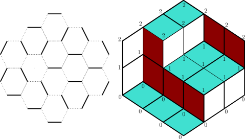
The other AKPZ growth models we mention below have the common feature of being defined in terms of dimer coverings of bipartite planar lattices (in particular, the honeycomb lattice and the square grid) or, equivalently, in terms of random tilings of the plane. It is a well-known fact [23] that dimer coverings of are in bijection with integer-valued height functions defined on the dual graph . See, e.g., Fig. 1 for lozenge tilings.
A general mechanism for obtaining AKPZ two-dimensional growth processes was suggested in [7], where the case of a particular continuous-time dynamics on the lozenge tilings of a half-plane was considered in detail as the main example (see also [8]). In this case, logarithmic growth of fluctuations in time and space was proven (whence ), the speed was computed, and the AKPZ signature was verified. The growth models generated by the procedure of [7] have the property of preserving families of Gibbs measures in certain unbounded regions of the plane. One can also prove that full-plane translation invariant Gibbs measures are stationary [33] (this requires extra non-trivial work because these dynamics involve unbounded particle jumps, which might cause the process to be ill-defined). A particular modification designed to preserve Gibbs measures inside bounded regions (hexagonal regions for lozenge tilings) was also suggested at the same time [10]. Other (discrete time) dynamics for lozenge tilings that fit into the formalism of [7] were considered in [3]; their speed of growth was computed there, and one can check that . Let us mention that an exposition of the general construction of [7] in terms of the formalism of Schur processes is available in [2] and another example for dimers on a square-hexagon lattice can be found in [9].
Another two-dimensional dynamics that recently attracted attention in the context of AKPZ growth model is the domino shuffling algorithm. While this evolution fits into the general framework of [7], it was actually introduced much earlier in [16, 29], as an algorithm that perfectly samples domino tilings of special domains of the plane called “Aztec diamonds”. However, the algorithm can be defined in more general domains: in particular, in the whole plane. Thanks to the above-mentioned mapping between a domino tiling and its discrete height function, the shuffling algorithm can be viewed as a two-dimensional growth model. In the whole plane, it preserves translation-invariant Gibbs measures of domino tilings. In the recent work [11], the shuffling algorithm was studied from the point of view of interface growth, and it was proven to belong to the AKPZ class, both in terms of vanishing of the growth exponents and in the sense that . An interesting fact observed in [11] is that, if the underlying dimer model is given non-uniform but periodic weights on , the speed function can be singular (non-differentiable) at isolated values of the slope (the case of weights with period in both space directions is worked out explicitly in [11]). At those slopes, growth exponents are still zero but the fluctuation variance is bounded in time and space.
We conclude this (incomplete) list of results by mentioning two more examples. The first one is an AKPZ growth model based on domino tilings in the plane, defined in Section 3.1 of [33], that at first sight does not seem to fit into the general formalism of [7]. The proof of logarithmic growth fluctuations, implying , as well as the computation of the speed of growth and a direct verification that can be found in [12]. The second one is the so-called -Whittaker process, introduced in [4] in the wider context of Macdonald processes. The -Whittaker dynamics reduces to the growth process of [7, 8] in the limit and to a Gaussian growth model (that has the same asymptotic large-scale behavior as the EW equation) in the limit [6, 5]. For every intermediate value of , it preserves certain Gibbs measures, both on the torus [14] and in certain unbounded domains of the plane. Logarithmic growth of fluctuations is not proven but conjectured.
For some of the models mentioned in this section, a hydrodynamic limit has been proven: the height profile, rescaled as , converges as to a non-random limit profile , that solves a first-order non-linear PDE of Hamilton-Jacobi type. See for instance [7, Th. 1.2] and [27] for a lozenge tiling dynamics, and [36] for the domino shuffling algorithm. Most likely, a similar convergence holds for the other models as well.
1.2. Preservation of Gibbs measures and of equilibrium shapes
A feature common to most (and possibly all) of the models cited in the previous section is that they admit certain translation-invariant Gibbs measures as stationary, but not reversible, measures for the height gradients (the law of the height itself is not stationary, since there is a non-zero average growth). In almost all of these models, Gibbs states have a determinantal (or free-fermion) structure, but this is not a general feature of AKPZ models: the -Whittaker process is not free-fermionic, for instance. The potential associated to these Gibbs measures is local and completely explicit: in several cases, for example for the lozenge dynamics of [7, 8], the Gibbs property means simply that, conditionally on the interface configuration outside any finite domain of the lattice, the configuration inside is uniformly distributed among all possible configurations compatible with . Actually, the general construction of [7] guarantees that these growth models preserve also non-translation invariant Gibbs measures, in the sense that if the initial condition is one such measure, then the law of the interface at a later time is another such measure (in general, a different one). See [7, Fig. 1.3] for a configuration sampled from one of these measure for lozenge tilings. Another example of preservation of non-translation-invariant Gibbs measure is provided by the domino shuffling algorithm: if at time the configuration is sampled from the Gibbs distribution in an Aztec diamond of size , at time it is distributed according to the Gibbs distribution in an Aztec diamond of size .
Preservation of Gibbs measures has a direct consequence on the hydrodynamic PDE of these growth models. To explain this, let us forget dynamics for a moment. According to the general principle of statistical mechanics, on large scales (i.e., rescaling height as and letting ), the height function sampled from a Gibbs measure concentrates around a non-random profile , the equilibrium shape. This profile is determined by minimizing a surface tension functional , with suitable boundary conditions. More explicitly, the function satisfies the Euler-Lagrange equation associated to such functional; due to convexity (see, e.g., [30, Ch. 4]) of the surface tension , this is a second-order PDE of elliptic type. Back to the growth models: the fact that the above AKPZ evolutions preserve Gibbs measures translates into the fact that their hydrodynamic PDE preserves the Euler-Lagrange equation. Namely, if the initial profile satisfies the Euler-Lagrange equation, then so does it at later times .
The main contribution of the present work, Theorem 2.1, is an elementary argument that shows that, roughly speaking, if the hydrodynamic PDE of a two-dimensional growth model preserves the Euler-Lagrange equation of some equilibrium interface model, then the speed of growth function satisfies . In the particular case where the growth model is defined in terms of lozenge tilings, or, more generally, in terms of a planar dimer model we show a stronger result (Theorems 3.2 and 3.3): the hydrodynamic PDE preserves the Euler-Lagrange equation of the dimer model if and only if the speed is a harmonic function with respect to a certain natural complex-valued variable defined in terms of the interface slope [24, 22].
We conclude this introduction with a couple of observations. First, we emphasize that Theorem 2.1 implies that the hydrodynamic PDE of Isotropic KPZ models, like the cube-stacking dynamics, cannot preserve the Euler-Lagrange equation of an equilibrium interface model with convex surface tension. This suggests the possibility that the stationary states of such growth processes are not of Gibbs type. The occurrence of non-Gibbs stationary states in irreversible interacting particle systems is believed to be a generic feature [26] but it has been proven only in very few examples (cf. Section 4.5.4 of [17] and references therein). Secondly, our argument might be instrumental in proving for some AKPZ models for which the explicit computation of is not possible. We think, in particular, of the above-mentioned -Whittaker process, whose invariant (Gibbs) measures are not of determinantal type and do not allow for explicit computations. A last remark is that, while in equilibrium statistical mechanics it is usually possible to guess the universality class a model belongs to from the symmetries of the Hamiltonian, for growth models it is not clear how to guess the convexity properties of from the definition of the generator.
2. Euler-Lagrange equation and AKPZ signature
From this point on, we denote macroscopic profiles (time-dependent as well as time-independent) by instead of , since the microscopic height will not appear in any of the subsequent arguments.
Let be the surface tension function of an equilibrium two-dimensional interface model, with denoting the surface tension at slope . We will denote by the derivative of w.r.t. components of , and by the matrix with
| (2.1) |
Since is convex, is positive definite (possibly not strictly). In many natural examples (notably the dimer model discussed in Section 3), the interface configurations are Lipschitz, and the allowed slopes belong to some convex set that in the dimer model setting is called “Newton Polygon”. In this case, equals outside and on the boundary of .
An “equilibrium shape” is a height profile that locally minimizes the surface tension functional
| (2.2) |
(One can also consider the optimization problem restricted to a sub-domain of the plane, in which case the boundary height on the boundary of is fixed.) More precisely, for every finite subset whose boundary is a smooth simple curve, the minimum of the functional
| (2.3) |
over functions on with boundary height is realized by the restriction of itself to . At every point where is , it satisfies the Euler-Lagrange equation
| (2.4) |
that is an elliptic PDE. While for solutions of the Euler-Lagrange equation are affine, this is not necessarily the case in dimension (and higher).
Now consider a two-dimensional growth model and assume it satisfies a hydrodynamic limit with speed function . Namely, its random height profile, once rescaled as explained at the end of Section 1.1, converges to the solution of the deterministic Hamilton-Jacobi equation
| (2.7) |
where is some function defined on the set of allowed slopes. Non-linear Hamilton-Jacobi equations like (2.7) are well-known to develop singularities (discontinuities of ) in finite time, and there is not a unique way of defining a weak solution after the time of appearance of singularities. However, the physically relevant solution defined for all times is the so-called viscosity solution [15], that can be obtained by adding to and then sending . We let denote the viscosity solution of (2.7) at time . We assume henceforth that is smooth enough so that the viscosity solution exists and is unique.
Our first result says, roughly speaking, that if the PDE (2.7) preserves the Euler-Lagrange equation (2.4), then the determinant of the Hessian of cannot be positive. More precisely:
Theorem 2.1.
Let be a slope in the interior of where both and are differentiable and where in (2.1) is strictly positive definite. Assume that there exists an equilibrium shape and a point where is differentiable, and such that:
-
•
and the Hessian of at is not zero;
-
•
one has
(2.8) for in a neighborhood of and sufficiently small.
Then, .
Proof.
For sufficiently small times the PDE (2.7) can be solved by the method of characteristics, and the solution is in the neighborhood of . Take that runs along the characteristic line started at , i.e.,
| (2.9) |
with the gradient of . Recall that is constant along the characteristic lines, so that is constant. Call
| (2.10) |
that equals zero by the assumption of the theorem.
Since is constant along characteristics, Eq. (2.10) gives
| (2.11) |
Using the chain rule for derivatives together with the definition (2.9) of characteristic lines we get
| (2.12) |
where
Altogether, we have obtained
| (2.13) |
with
| (2.14) |
For lightness of notation, call the Hessian matrix of computed at and write instead of . Assume by contradiction that and that is positive definite (the argument works analogously if and is negative definite), so that we can write it as . Also call the vector . We rewrite (2.13) as
Since the matrix is strictly positive definite,
By the assumption that the Hessian of at is non-zero, either or is non-zero. If one of them, say , is zero, then one gets
| (2.15) |
so that is not strictly positive definite, which is a contradiction. Also, if either or is zero, then again which contradicts the hypothesis . From now on we can therefore assume that . Also, cannot be orthogonal to ; otherwise
which is not possible since . In the remaining case where ,
| (2.16) |
that is a contradiction. Altogether, it is not possible that . ∎
3. Dimer model: Burgers equation and harmonicity of
In this section, we assume that is the surface tension of a dimer model on a bipartite, planar, periodic graph. We refer, e.g., to [23] for an introduction to dimer models and to [25] for the definition of their ergodic Gibbs measures; we recall here a minimum of basic facts. Given a planar, bipartite, periodic weighted graph (positive weights are associated to edges), dimer configurations are perfect matchings of , and a canonical construction allows to associate to a dimer configuration an integer-valued height function on faces of (the map is bijective up to a global additive constant for the height). The possible slopes of the height function belong to a convex polygon , called “Newton polygon”, whose vertices have integer coordinates. For every slope in the interior of there exists a unique translation invariant, ergodic Gibbs measure on dimer coverings, with average slope . Conditionally on the dimer configuration outside any finite sub-graph , assigns to any admissible dimer configuration in a probability proportional to the product of weights of edges occupied by dimers. Slopes that are in the interior of and whose coordinates are not both integer are called “liquid slopes”. In this case, is called a “liquid phase” and it is known that dimer correlations decay polynomially and the height field behaves like a log-correlated massless Gaussian field on large scales. If is in the interior of but has integer coordinates, then for generic choice of the edge weights the measure is a “gaseous” or “smooth” phase, with exponentially decaying correlations and height fluctuations222For special edge weights, the measure can be liquid (with polynomially decaying correlations) even for integer-valued slopes [25]. . A crucial object for the dimer model is the so-called characteristic polynomial : this is a Laurent polynomial in , that is associated to the weighted graph . For instance, the surface tension is obtained as the Legendre transform with respect of of
| (3.1) |
For the dimer model, it is known that the Euler-Lagrange equations (2.4) for equilibrium shapes can be expressed via a first-order PDE, that was called complex Burgers equation in [24]. Namely, for , define non-zero complex numbers via the relations333Our correspond to the complex conjugates of the similarly denoted complex numbers in [24].
| (3.2) |
According to [24, Theorem 1], at every point in the liquid region (i.e., such that in the neighborhood of , is with a liquid slope), the Euler-Lagrange equation (2.4) is equivalent to the “complex Burgers equation”
| (3.3) |
where denotes the derivative of w.r.t. . Note that relation (3.2) does not really fix because the argument is a multi-valued function; as explained in [24], the statement is that there exists a branch of the argument for which equality (3.2) is satisfied.
Take a point in the liquid region, where the gradient of is
| (3.4) |
for some such that . Locally around we can expand as
| (3.5) |
with . As discussed in [24, Sec. 2.3], the ratio is neither zero nor infinite. Then, by the implicit function theorem we can locally write as a differentiable function or, conversely, write as a differentiable function .
An identity that will be important in the following is that
| (3.6) |
that follows from [24, Eq. (12)]. We have also
| (3.7) |
that follow from (3.2).
Relations and (3.2) give a bijection between in a neighborhood of and the interface slope in a neighborhood of . Therefore, we can write locally (i.e., for close to ) the speed as some function .
Remark 3.1.
Globally, the mapping from to the slope is multi-valued, since for a given there may be many satisfying . Notable exceptions are the dimer model on the honeycomb lattice and the square grid with translation-invariant weights. We will briefly come back to these special cases in Section 3.1. See instead [11] for a growth model in a case where the solution of has several branches.
Let be the viscosity solution of the PDE (2.7). For small and around the solution is smooth, and we let be defined by (3.2) with replaced by , with a choice of the branch of the argument so that . Define also
| (3.8) |
so that iff the complex Burgers equation (3.3) holds.
Theorem 3.2.
Conversely, we have:
Theorem 3.3.
The restriction to small times is simply due to the fact that at large times the solution might not be pointwise differentiable in space and time, in which case is not well defined.
Remark 3.4.
Proof of Theorems 3.2 and 3.3.
We start by writing
| (3.10) |
where we used and . Also,
| (3.11) |
In the second step we used (3.6), in the third the identities
| (3.12) | |||||
and in the last (3.7).
Note that, writing and recalling the definition (3.8) of , one has
| (3.13) |
so that
| (3.14) |
because
Together with (3.10), (3.11), (3.12), we obtain
| (3.15) |
with and
| (3.16) |
Similarly, one gets
with
| (3.17) |
From (3.8) we see that
| (3.18) |
Computing the derivatives in (3.18) and simplifying, one is left in the end with
| (3.19) |
that is the main achievement of the computation.
Let us prove Theorem 3.2. By assumption, is zero at time zero and is also zero, so that
| (3.20) |
Note that vanishes only if is real. On the other hand, (3.13) implies that if then
| (3.21) |
and, as shown in [24, Sec. 2.3], the r.h.s. belongs to . The claim of the theorem then follows.
As for Theorem 3.3, recall from definitions (3.16) and (3.17) that are linear in and that is harmonic by assumption. If we consider as known functions of space and time, then one sees that the r.h.s. of (3.19) is Lipschitz in and its derivatives w.r.t. . As long as is sufficiently regular in space and time so that all derivatives exist, we see that remains zero if it is zero initially, as it is the solution of an initial value problem with Lipschitz right-hand side.
∎
3.1. A couple of concrete examples
For the dimer model on the honeycomb lattice with uniform weights, the characteristic polynomial is [23] and (with a conventional choice of coordinates on the honeycomb lattice) the Newton polygon is the triangle with vertices . The condition implies , and the mapping from to induced by (3.2) is a bijection from the upper half complex plane to . The -to-slope mapping is illustrated in Figure 2.

Some of the two-dimensional growth models mentioned in the introduction, notably those defined in [7] and [3], are known to preserve the Gibbs measures of the honeycomb dimer model. For these models, the speed of growth turns out to be a harmonic function of that, once expressed in terms of , can be checked by direct computation to have AKPZ signature: . Thanks to our Theorems 3.3 and 2.1, AKPZ signature follows simply by harmonicity.
Another natural example is when is the square grid with unit weights. With a natural choice of Kasteleyn matrix one finds the characteristic polynomial
Then, gives , and one easily checks that relations (3.2) give again a bijection between the upper half-plane and the Newton polygon, that in this case is the square with vertices . See Fig. 3 and also the discussion in [12, Sec. 2.4 and Fig. 3]. As we mentioned in the introduction, the two-dimensional domino-tiling growth model defined in Section 3.1 of [33] admits the Gibbs measures of the dimer model on as stationary states. The speed of growth was computed in [12]: while it has quite a complicated expression in terms of , see [12, Eq. (2.6)], once expressed in terms of it equals just . In [12, App. B], a lengthy but direct computation shows that ; again, this can be obtained as an immediate consequence of our present results.

Acknowledgements
We are grateful to Rick Kenyon, Senya Shlosman and Herbert Spohn for very helpful suggestions. A.B. was partially supported by the NSF grant DMS-1607901 and DMS-1664619. F.T. was partially supported by the CNRS PICS grant “Interfaces aléatoires discrètes et dynamiques de Glauber”, by ANR-15-CE40-0020-03 Grant LSD and by MIT-France Seed Fund “Two-dimensional Interface Growth and Anisotropic KPZ Equation”.
References
- [1] A.-L. Barabási and H. E. Stanley, Fractal concepts in surface growth, Cambridge University Press, 1995.
- [2] A. Borodin, Schur dynamics of the Schur processes, Advances in Mathematics, 228 (2011), 2268-2291.
- [3] A. Borodin, A. Bufetov and G. Olshanski, Limit shapes for growing extreme characters of , Ann. Appl. Probab. 25 (2015), 2339-2381.
- [4] A. Borodin, I. Corwin, Macdonald processes, Probab. Theory Relat. Fields 158 (2014), 225-400.
- [5] A. Borodin, I. Corwin, P. L. Ferrari, Anisotropic (2+1)d growth and Gaussian limits of q-Whittaker processes, Probab. Theory Rel. Fields, Online First, arXiv:1612.00321.
- [6] A. Borodin, I. Corwin, F. L. Toninelli, Stochastic heat equation limit of a -D growth model, Comm. Math. Phys. 350 (2017), 957-984.
- [7] A. Borodin and P. L. Ferrari, Anisotropic Growth of Random Surfaces in Dimensions, Comm. Math. Phys., 325 (2014), 603-684.
- [8] A. Borodin, P. L. Ferrari, Anisotropic growth of random surfaces in 2+1 dimensions: fluctuations and covariance structure. J. Stat. Mech. P02009 (2009).
- [9] A. Borodin, P. L. Ferrari, Random tilings and Markov chains for interlacing particles, arXiv:1506.03910.
- [10] A. Borodin, V. Gorin, Shuffling algorithm for boxed plane partitions, Adv. Math. 220 (2009), 1739-1770.
- [11] S. Chhita, F. Toninelli, A -dimensional Anisotropic KPZ growth model with a rigid phase, arXiv:1802.05493.
- [12] S. Chhita, P. L. Ferrari, F. Toninelli, Speed and fluctuations for some driven dimer models, to appear on Ann. Inst. H. Poincaré D, arXiv:1705.07641.
- [13] I. Corwin, Macdonald processes, quantum integrable systems and the Kardar-Parisi-Zhang universality class, Proc. of the ICM Seoul 2014, vol. 3, 1007-1034.
- [14] I. Corwin, F. L. Toninelli, Stationary measure of the driven two-dimensional -Whittaker particle system on the torus, Electron. Commun. Probab. 21 (2016).
- [15] M. G. Crandall, H. Ishii and P. L. Lions, User’s guide to viscosity solutions of second order partial differential equations, Bulletin of the American Mathematical Society, 27 (1) (1992), 1-67.
- [16] N. Elkies, G. Kuperberg, M. Larsen and J. Propp, Alternating-sign matrices and domino tilings, J. Algebraic Combin. 1 (1992), 111-132.
- [17] A.C.D. van Enter, R. Fernández and A.D. Sokal, Regularity properties and pathologies of position- space renormalization-group transformations: Scope and limitations of Gibbsian theory, J. Stat. Phys. 72, 879-1167, (1993).
- [18] D. J. Gates and M. Westcott, Stationary states of crystal growth in three dimensions, J. Stat. Phys. 81 (1995), 681-715.
- [19] T. Halpin-Healy and A. Assdah, On the kinetic roughening of vicinal surfaces, Phys. Rev. A, 46 (1992), 3527–3530.
- [20] T. Halpin-Healy, G. Palasantzas, Universal correlators & distributions as experimental signatures of -dimensional Kardar-Parisi-Zhang growth, Europhys. Lett. 105, 50001 (2014).
- [21] M. Kardar, G. Parisi, and Y. C. Zhang, (1986). Dynamic scaling of growing interfaces, Physical Review Letters 56 (1986), 889.
- [22] R. Kenyon, Height fluctuations in the honeycomb dimer model, Comm. Math. Phys. 281 (2008), 675-709
- [23] R. Kenyon, Lectures on dimers, In Statistical mechanics, volume 16 of IAS/Park City Math. Ser., pages 191-230. Amer. Math. Soc., Providence, RI, 2009.
- [24] R. Kenyon, A. Okounkov, Limit shapes and the complex Burgers equation, Acta Math. 199 (2007), 263-302.
- [25] R. Kenyon, A. Okounkov, and S. Sheffield, Dimers and amoebae, Ann. of Math., 163 (2006), 1019-1056.
- [26] J. L. Lebowitz and R. H. Schonmann, Pseudo-free energies and large deviations for non-Gibbsian FKG measures. Prob. Th. Rel. Fields 77 (1988), 49-64.
- [27] M. Legras, F. L. Toninelli, Hydrodynamic limit and viscosity solutions for a 2D growth process in the anisotropic KPZ class, to appear on Comm. Pure Appl. Math., arXiv:1704.06581.
- [28] M. Prähofer and H. Spohn, An Exactly Solved Model of Three Dimensional Surface Growth in the Anisotropic KPZ Regime, J. Stat. Phys. 88 (1997), 999-1012.
- [29] J. Propp, Generalized Domino-Shuffling, Theoret. Comput. Sci., 303 (2003), 267-301.
- [30] S. Sheffield, Random surfaces, Astérisque (2005).
- [31] T. Seppäläinen, Strong law of large numbers for the interface in ballistic deposition, Annales Inst. H. Poincaré: Prob. Stat. 36 (2000), 691-736.
- [32] L.-H. Tang, B. M. Forrest, D. E. Wolf, Kinetic surface roughening. II. Hypercube stacking models, Phys. Rev. A 45 (1992), 7162-7169.
- [33] F. L. Toninelli, A -dimensional growth process with explicit stationary measures, Ann. Probab. 45 (2017), 2899-2940.
- [34] F. L. Toninelli, -dimensional interface dynamics: mixing time, hydrodynamic limit and Anisotropic KPZ growth, to appear on Proc. of the ICM Rio de Janeiro 2018, arXiv:1711.05571.
- [35] D. E. Wolf, Kinetic roughening of vicinal surfaces, Phys. Rev. Lett. 67 (1991), 1783-1786.
- [36] X. Zhang, Domino shuffling height process and its hydrodynamic limit, preprint.