Effective quantum Zeno dynamics in dissipative quantum systems

Abstract

We investigate the time evolution of an open quantum system described by a Lindblad master equation with dissipation acting only on a part of the degrees of freedom ${\cal H}_{0}$ of the system, and targeting a unique dark state in ${\cal H}_{0}$. We show that, in the Zeno limit of large dissipation, the density matrix of the system traced over the dissipative subspace ${\cal H}_{0}$, evolves according to another Lindblad dynamics, with renormalized effective Hamiltonian and weak effective dissipation. This behavior is explicitly checked in the case of Heisenberg spin chains with one or both boundary spins strongly coupled to a magnetic reservoir. Moreover, the populations of the eigenstates of the renormalized effective Hamiltonian evolve in time according to a classical Markov dynamics. As a direct application of this result, we propose a computationally-efficient exact method to evaluate the nonequilibrium steady state of a general system in the limit of strong dissipation.

I Introduction

A quantum system interacting with an environment is, under a Markov assumption, well described by a Lindblad master equation (LME) Lindblad (1976); Gorini et al. (1976). It follows that the reduced density matrix (RDM) of the system undergoes a coherent and dissipative evolution Breuer and Petruccione (2002); Clark et al. (2010). If the coherent and dissipative parts of LME do not depend on time, then, after a transient, the system reaches a (unique) nonequilibrium steady state (NESS), which is independent of the initial conditions. Even if the NESS is trivial, the relaxation dynamics may not be: specially if a large dissipation-free subspace exists, the NESS can be approached through a complicated multi-stage evolution.

If the dissipation time-scales are short in comparison with the coherent evolution times, then the so-called quantum Zeno regime occurs. Quantum Zeno effect Misra and Sudarshan (1977); Koshino and Shimizu (2005) predicts an inhibition of quantum transitions in a quantum system subjected to frequent measurements. It has been observed experimentally, in various setups Itano et al. (1990); Kwiat et al. (1995); Signoles et al. (2014); Schäfer et al. (2014); Patil et al. (2015). Applications of Zeno effect include dissipation-protected realization of quantum gates Beige et al. (2000), engineering of nontrivial quantum states and implementation of universal quantum computations Verstraete et al. (2009); Yi et al. (2012); Elliott et al. (2015); Winkler et al. (2006) creating quantum simulators Stannigel et al. (2014), localization of a single atom in a lattice Ashida and Ueda (2015), realization of exotic effective dynamics Lee and Ruostekoski (2014); Elliott and Mekhov (2016), development of theoretical tools for a real-time observation of quantum many-body dynamics Ashida and Ueda (2017).

It is well recognized that the evolution of a system near the Zeno limit is not frozen but can proceed via Raman-like processes involving virtual levels, which couple states within a given Zeno subspace Kozlowski et al. (2016); Elliott and Vedral (2016), while the occupation of the virtual levels remains negligible.

In more details, one can distingish three stages of relaxation, occurring at different time scales. On the shortest time scale, only the degrees of freedom directly affected by the dissipation, relax to their stationary values. On the second, intermediate time scale, an effective coherent evolution takes place, governed by a dissipation-projected Hamiltonian Zanardi and Campos Venuti (2014). Finally, on the longest time scale, all system characteristics relax to their stationary values.

In this paper, we focus on the third stage of evolution and derive an effective dynamics of the system in the decoherence-free subspace. It happens that, in the assumed Zeno regime, and under the non-degeneracy assumption for the local kernel of the dissipator (2), this dynamics is also of Lindblad type. As an application, we demonstrate that the spectrum of the reduced density matrix, which does not change on the intermediate time scale, on the longest time scale evolves according to a classical Markov process, with generator $F$ computable from the LME entries.

II Main results

Consider an open quantum system, with finite Hilbert space ${\cal H}$, under strong dissipation acting only on a subspace $\mathcal{H}_{0}$ of the degrees of freedom, described by the Lindblad master equation,

$$\frac{\partial\rho(\tau)}{\partial\tau}=-\frac{i}{\hbar}\left[H,\rho(\tau)\right]+\Gamma{\cal D}[\rho(\tau)].$$ (1)

Let the dissipation-free subspace be ${\cal H}_{1}$, ${\cal H}={\cal H}_{0}\otimes{\cal H}_{1}$, and denote by $\mathop{\mathrm{tr}_{\mathcal{H}_{0}}}\limits$ and $\mathop{\mathrm{tr}_{\mathcal{H}_{1}}}\limits$ the trace over $\mathcal{H}_{0}$ and $\mathcal{H}_{1}$, having dimensions $d_{0}$ and $d_{1}$, respectively. We assume the Lindblad dissipator $\mathcal{D}$ to target a unique state $\psi_{0}\in\mathcal{H}_{0}$, namely,

$$\left(\mathop{\mathrm{tr}_{\mathcal{H}_{1}}}\limits\mathcal{D}\right)\psi_{0}=0.$$ (2)

The aim of this paper is to show that, in the Zeno limit, when the effective dissipation strength $\Gamma$ is much stronger than the unitary part of the evolution, the solution of the problem (1) for all times $\tau>O(1)$ has the approximate form

$$\rho(\tau)=\psi_{0}\otimes R(\tau),$$

where $R(\tau)=\mathop{\mathrm{tr}_{\mathcal{H}_{0}}}\limits\rho(\tau)$ evolves according to another LME

$$\frac{\partial R(\tau)}{\partial\tau}=-\frac{i}{\hbar}\left[\tilde{H},R(\tau)\right]+\frac{1}{\Gamma}\tilde{\mathcal{D}}[R(\tau)].$$ (3)

More precisely, we demonstrate that

$$\|\rho(\tau)-\psi_{0}\otimes R(\tau)\|=O\left(\frac{1}{\Gamma}\right),$$ (4)

for $\Gamma\to\infty$ and for all times $\tau\gg 1/\Gamma$. The choice of the norm $\|\cdot\|$ is rather arbitrary. Note that the LMEs (1) and (3), besides being defined in terms of different Hamiltonians and dissipators, have dissipation strength $\Gamma$ and $1/\Gamma$, respectively.

Using $1/\Gamma\ll 1$ as a small parameter, we obtain the above result by writing the Dyson series for the Liouvillian dynamics associated to the LME (1). We start rescaling the time $\Gamma\tau=t$ in the original LME. In the limit of strong dissipation $\Gamma\gg 1$, we obtain an equation with a perturbative term,

$$\frac{\partial\rho}{\partial t}=\mathcal{D}[\rho]-\frac{i}{\Gamma}\left[H,\rho\right]=(\mathcal{L}_{0}+K)\rho=\mathcal{L}\rho,$$ (5)

where $\mathcal{L}=\mathcal{L}_{0}+K$ and the linear operators $\mathcal{L}_{0}$ and $K=-(i/\Gamma)\left[H,\cdot\right]$ denote the dissipator and the commutator, respectively. The formal solution of Eq. (5) is

$$\rho(t)=e^{\mathcal{L}t}\rho(0)=\mathcal{E}(t)\rho(0),$$ (6)

where the propagator $\mathcal{E}(t)$ satisfies

$$\mathcal{E}(t)=e^{\mathcal{L}_{0}t}\left(1+\int_{0}^{t}dt_{1}e^{-\mathcal{L}_{0}t_{1}}K\mathcal{E}(t_{1})\right).$$ (7)

Iterating Eq. (7) we get the Dyson expansion. Up to the second order we obtain

$$\mathcal{E}(t)= \ e^{\mathcal{L}_{0}t}\left(1+\int_{0}^{t}\!\!\!dt_{1}e^{-\mathcal{L}_{0}t_{1}}Ke^{\mathcal{L}_{0}t_{1}}\right.$$

$$+\left.\int_{0}^{t}\!\!\!dt_{1}e^{-\mathcal{L}_{0}t_{1}}Ke^{\mathcal{L}_{0}t_{1}}\int_{0}^{t_{1}}\!\!\!dt_{2}e^{-\mathcal{L}_{0}t_{2}}Ke^{\mathcal{L}_{0}t_{2}}+\dots\right).$$ (8)

Introduce the spectral projection $\mathcal{P}_{0}$ onto the kernel of the dissipator $\mathcal{L}_{0}$, namely, $\mathcal{P}_{0}=\lim_{t\rightarrow\infty}\exp(\mathcal{L}_{0}t)$. Define also its complement $\mathcal{Q}_{0}=I_{\mathcal{H}}-\mathcal{P}_{0}$, where $I_{\mathcal{H}}$ is the identity operator in the space $\mathcal{H}$. Obviously, $\mathcal{P}_{0}\mathcal{Q}_{0}=0$. If $1/\Gamma$ is small, the dissipative part of the Lindbladian constrains the system to a decoherence-free subspace. In fact, the leakage outside of decoherence-free subspace (defined as the subspace belonging to the dissipator Kernel) can be rigorously proven to be negligible, see Ref. Zanardi and Campos Venuti (2014). Therefore, we shall only consider an evolution inside the decoherence-free subspace, which is given by the propagator $\mathcal{P}_{0}\mathcal{E}(t)\mathcal{P}_{0}$. Performing the calculations as indicated in Appendix A, we obtain

$$\mathcal{P}_{0}\mathcal{E}(t)\mathcal{P}_{0}= \ \mathcal{P}_{0}+t\mathcal{P}_{0}K\mathcal{P}_{0}+\frac{t^{2}}{2!}(\mathcal{P}_{0}K\mathcal{P}_{0})^{2}$$

$$-t\mathcal{P}_{0}K\mathcal{Q}_{0}\mathcal{S}K\mathcal{P}_{0}+\ldots,$$ (9)

where $\ldots$ is the contribution from the remaining orders of the Dyson expansion, and $\mathcal{S}$ is the pseudo-inverse of the dissipator,

$$\mathcal{L}_{0}\mathcal{S}=\mathcal{S}\mathcal{L}_{0}=\mathcal{Q}_{0}.$$ (10)

Note that the first three terms in Eq. (9) can be exponentiated, as $\mathcal{P}_{0}\exp(t\mathcal{P}_{0}K\mathcal{P}_{0})$. They all describe a unitary dynamics within the decoherence-free subspace, as is seen by applying the propagator $\mathcal{P}_{0}K\mathcal{P}_{0}$ on a state $\rho=\psi_{0}\otimes R$,

$$\mathcal{P}_{0}K\mathcal{P}_{0}\rho =-\frac{i}{\Gamma}\mathcal{P}_{0}[H,\psi_{0}\otimes R]$$

$$=-\frac{i}{\Gamma}\psi_{0}\otimes\mathop{\mathrm{tr}_{\mathcal{H}_{0}}}\limits\left(H(\psi_{0}\otimes R)-(\psi_{0}\otimes R)H\right)$$

$$=-\frac{i}{\Gamma}\psi_{0}\otimes\left[h_{D},R\right],$$ (11)

where $h_{D}$ is the dissipation-projected Hamiltonian

$$h_{D}=\mathop{\mathrm{tr}_{\mathcal{H}_{0}}}\limits\left(\left(\psi_{0}\otimes I_{\mathcal{H}_{1}}\right)H\right).$$ (12)

Since the operator $K$ is proportional to the small parameter $1/\Gamma$, we conclude that the terms $t\mathcal{P}_{0}K\mathcal{P}_{0}$ and $\frac{t^{2}}{2!}(\mathcal{P}_{0}K\mathcal{P}_{0})^{2}$ give a contribution $O(1)$ to the propagator for times $t\sim O(\Gamma)$, while the last term $-t\mathcal{P}_{0}K\mathcal{Q}_{0}\mathcal{S}K\mathcal{P}_{0}$ contributes $O(1)$ changes to the propagator for $t\sim O(\Gamma^{2})$. The physical interpretation of Eq. (9) is thus as follows. One observes three different processes, taking place at different time scales $\tau=t/\Gamma$: (i) at short times $\tau\sim 1/\Gamma$, the system is projected onto the decoherence-free subspace; (ii) at intermediate times $\tau\sim 1$, the evolution inside the decoherence-free subspace is unitary $\mathcal{P}_{0}K\mathcal{P}_{0}\sim-i\psi_{0}\otimes[h_{D},\cdot]$; (iii) at large times $\tau\sim\Gamma$ the term $t\mathcal{P}_{0}K\mathcal{Q}_{0}\mathcal{S}K\mathcal{P}_{0}$ sets in. Note that the slowest part of the evolution, taking place at the longest time scale, cannot by any means be ignored since it is the only part containing a relaxation towards the NESS. In fact, the unitary evolution alone governed by the effective Hamiltonian (12), does not lead to any relaxation.

To derive the evolution equation from the Dyson expansion, assume the system to start in the dissipation-free subspace, i.e., $\rho(0)=\mathcal{P}_{0}\rho(0)$. This is equivalent to assuming the factorized initial state $\rho(0)=\psi_{0}\otimes R(0)$. The time evolution inside the decoherence-free subspace is given by $\mathcal{P}_{0}\mathcal{E}(t)\mathcal{P}_{0}[\psi_{0}\otimes R(0)]=\psi_{0}\otimes R(t)$. We obtain the evolution equation in differential form considering $\lim_{t\rightarrow 0}[\rho(t)-\rho(0)]/t=\partial\rho/\partial t$. Using the Dyson expansion, tracing over $\mathcal{H}_{0}$, and rescaling the time $t/\Gamma=\tau$, we obtain

$$\frac{\partial R}{\partial\tau} =-i\left[h_{D},R(\tau)\right]+\frac{1}{\Gamma}W$$ (13)

$$W =-\Gamma^{2}\mathop{\mathrm{tr}_{\mathcal{H}_{0}}}\limits\left(\mathcal{P}_{0}K\mathcal{Q}_{0}SK\mathcal{P}_{0}\rho\right)$$ (14)

Equation (13) is valid for time scales beyond the shortest one, i.e., $\tau\gg 1/\Gamma$. The total error of the effective description (13) of the evolution $\rho(0)\rightarrow\rho(\tau)\approx\psi_{0}\otimes R(\tau)$ for large $\Gamma$ results from two contributions: a leakage outside the dissipation-free subspace and higher order dissipation terms, both contributions being generically of order $1/\Gamma$, see also Fig. 1.

To evaluate $W$ from Eq. (14), we make two assumptions: (i) the kernel of $\mathcal{L}_{0}$ is one-dimensional, i.e., the eigenvalue $0$ of the dissipator is non-degenerate,

$$\mathcal{L}_{0}\psi_{0} =0;$$ (15)

(ii) $\mathcal{L}_{0}$ is diagonalizable, i.e., a basis $\psi_{k}$ (not necessarily orthogonal) exists,

$$\mathcal{L}_{0}\psi_{k} =\xi_{k}\psi_{k}.$$ (16)

Note that $\psi_{k}^{\dagger}$ are also eigenvectors of the dissipator, with eigenvalues $\xi_{k}^{*}$, namely, $\mathcal{L}_{0}\psi_{k}^{\dagger}=\xi_{k}^{*}\psi_{k}^{\dagger}$. We also introduce a complementary basis $\varphi_{k}$, trace-orthonormal to the basis $\psi_{j}$,

$$\mathop{\mathrm{tr}}\limits(\varphi_{k}\psi_{j}) =\delta_{k,j}.$$ (17)

Hereafter, we work in the representation in which $\psi_{k},\varphi_{k}$ are square matrices.

First, we note that the action of $\mathcal{P}_{0}$ on the arbitrary element $X\in\mathcal{H}$ is

$$\mathcal{P}_{0}X =\psi_{0}\otimes\mathop{\mathrm{tr}_{\mathcal{H}_{0}}}\limits X.$$ (18)

In fact, due to the definition of $\mathcal{P}_{0}$ we have

$$\mathcal{P}_{0}X =\lim_{t\rightarrow\infty}e^{\mathcal{L}_{0}t}X=\lim_{t\rightarrow\infty}e^{\mathcal{L}_{0}t}\sum_{k}\psi_{k}\otimes x_{k}$$

$$=\sum_{k}\lim_{t\rightarrow\infty}e^{\xi_{k}t}\psi_{k}\otimes x_{k}=\psi_{0}\otimes x_{0},$$ (19)

since the real part of all $\xi_{k}$ for $k>0$ is strictly negative. In the decomposition $X=\sum_{k}\psi_{k}\otimes x_{k}$, the element $x_{0}$ can be found using the trace-orthonormal basis $\varphi_{k}$ as $x_{0}=\mathop{\mathrm{tr}_{\mathcal{H}_{0}}}\limits(\varphi_{0}\otimes I_{\mathcal{H}_{1}})X$. The element $\varphi_{0}$ of this basis, satisfying $\mathop{\mathrm{tr}}\limits(\varphi_{0}\psi_{k})=\delta_{k,0}$, can always be chosen as the unit matrix, $\varphi_{0}=I_{\mathcal{H}_{0}}$, since all the eigenfunctions of the dissipator with nonzero eigenvalues are traceless, and $\mathop{\mathrm{tr}}\limits\psi_{0}=1$. Substituting $x_{0}=\mathop{\mathrm{tr}_{\mathcal{H}_{0}}}\limits X$ in Eq. (19), we obtain Eq. (18).

It is convenient to define the Hamiltonian decomposition

$$H =\sum_{n}\varphi_{n}\otimes g_{n}=\sum_{n}\varphi_{n}^{\dagger}\otimes g_{n}^{\dagger},$$ (20)

$$g_{k} =\mathop{\mathrm{tr}_{\mathcal{H}_{0}}}\limits((\psi_{k}\otimes I_{\mathcal{H}_{1}})H).$$ (21)

We have, step by step,

$$\mathcal{P}_{0}\rho(0) =\rho(0),$$

$$(\Gamma K)\mathcal{P}_{0}\rho(0) =-i\left[H,\rho(0)\right]$$

$$=-i\sum_{m,n}\left(C_{mn}\psi_{m}^{\dagger}\otimes(g_{n}R)-\mathrm{H.c.}\right),$$

$$\mathcal{Q}_{0}S(\Gamma K)\mathcal{P}_{0}\rho(0) =-i\!\!\!\sum_{m>0,n}\frac{1}{\xi_{m}^{*}}\left(C_{mn}\psi_{m}^{\dagger}\otimes(g_{n}R)-\mathrm{H.c.}\right),$$

where

$$C_{mn} =\mathop{\mathrm{tr}}\limits\left(\varphi_{m}^{\dagger}\varphi_{n}\psi_{0}\right).$$ (22)

Since $\varphi_{0}=I_{\mathcal{H}_{0}}$, the coefficients $C_{mn}$ satisfy

$$C_{0n} =C_{n0}=\delta_{0,n}.$$ (23)

In the last step, using Eqs. (17) and (18), we arrive at

$$W =\!\!\!\!\sum_{m>0,n>0}\left(\frac{C_{mn}}{-\xi_{m}^{*}}\left(-g_{m}^{\dagger}g_{n}R+g_{n}Rg_{m}^{\dagger}\right)+\mathrm{H.c.}\right).$$ (24)

Note that the term $n=0$ does not appear in the sum (24) because of Eq. (23). Using the substitution $-C_{mn}/\xi_{m}^{*}=Y_{mn}=A_{mn}/2+iB_{mn}$ with $A_{mn}=Y_{mn}+Y_{nm}^{*}$ positive matrix and $B_{mn}=(Y_{mn}-Y_{nm}^{*})/(2i)$ Hermitian matrix, and changing the order of summation in the H.c. term in (24), we can put $W$ in the general Lindbladian form,

$$W=-i[\tilde{H}_{a},R]+\tilde{\mathcal{D}}R,$$ (25)

$$\tilde{H}_{a}=\!\!\!\!\!\!\sum_{m>0,n>0}\!\!\!\!\!B_{mn}g_{m}^{\dagger}g_{n},$$ (26)

$$\tilde{\mathcal{D}}R=\!\!\!\!\!\!\sum_{m>0,n>0}\!\!\!\!\!A_{mn}\left(g_{n}Rg_{m}^{\dagger}-\frac{1}{2}g_{m}^{\dagger}g_{n}R-\frac{1}{2}Rg_{m}^{\dagger}g_{n}\right).$$ (27)

According to Eq. (13), from the above expression of $W$ we conclude that the effective time evolution of the system in the dissipation-free subspace has the standard Lindblad form of Eq. (3), with $\tilde{H}=h_{D}+\tilde{H}_{a}/\Gamma$ and the dissipator $\tilde{\mathcal{D}}/\Gamma$ with $\tilde{\mathcal{D}}$ given by Eq. (27). Note that the stronger is the dissipation $\Gamma$ in the original system, the weaker is the effective dissipation (of order $1/\Gamma$) in the effective dynamics Carollo et al. (2006).

III Heisenberg spin chain with the first spin in a target state

To illustrate our findings, we consider a system of interacting spins, with one spin strongly dissipatively coupled to an environment which targets an arbitrary mixed state $\psi_{0}$ of that spin. In the Lindblad formalism, this is achieved via the application of two Lindblad operators Prosen (2011),

$$L_{1}=\sqrt{\frac{1+\mu}{2}}|0^{\perp}\rangle\langle 0|,\qquad L_{2}=\sqrt{\frac{1-\mu}{2}}|0\rangle\langle 0^{\perp}|,$$ (28)

where $|0\rangle$ is an arbitrary normalized state in $\mathcal{H}_{0}\equiv\mathbb{C}_{2}$, $\left\langle 0^{\perp}|0\right\rangle=0$ and $\mu$ real parameter with $0\leq\mu\leq 1$. The resulting dissipator $\mathcal{L}_{0}=\mathcal{D}_{L_{1}}+\mathcal{D}_{L_{2}}$, where

$$\mathcal{D}_{L}X =LXL^{\dagger}-\frac{1}{2}(L^{\dagger}LX+XL^{\dagger}L),$$ (29)

targets the arbitrary mixed state of a single spin

$$\psi_{0}=\frac{1+\mu}{2}|0\rangle\langle 0|+\frac{1-\mu}{2}|0^{\perp}\rangle\langle 0^{\perp}|.$$ (30)

In fact, $\psi_{0}$ is an eigenvector of the dissipator $\mathcal{L}_{0}$ with eigenvalue $\xi_{0}=0$, namely, $\mathcal{L}_{0}\psi_{0}=0$. The other eigenvectors and the corresponding eigenvalues of $\mathcal{L}_{0}$ are

$$\psi_{1} =|0\rangle\langle 0^{\perp}|,\qquad\xi_{1}=-\frac{1}{2},$$ (31)

$$\psi_{2} =|0^{\perp}\rangle\langle 0|,\qquad\xi_{2}=-\frac{1}{2},$$ (32)

$$\psi_{3} =|0\rangle\langle 0|-|0^{\perp}\rangle\langle 0^{\perp}|,\qquad\xi_{3}=-1.$$ (33)

The trace-orthonormal basis $\varphi_{k}$ satisfying $\mathop{\mathrm{tr}}\limits(\varphi_{k}\psi_{m})=\delta_{k,m}$ is given by

$$\varphi_{0} =I_{\mathbb{C}_{2}},$$ (34)

$$\varphi_{1} =|0^{\perp}\rangle\langle 0|,$$ (35)

$$\varphi_{2} =|0\rangle\langle 0^{\perp}|,$$ (36)

$$\varphi_{3} =\frac{1-\mu}{2}|0\rangle\langle 0|-\frac{1+\mu}{2}|0^{\perp}\rangle\langle 0^{\perp}|.$$ (37)

Given the explicit form of $\varphi_{k},\psi_{k}$, we readily compute the coefficients $C_{mn}$ from Eq. (22). The only nonzero coefficients $C_{mn}$ are the diagonal ones: $C_{00}=1$, $C_{11}=(1+\mu)/2$, $C_{22}=(1-\mu)/2$, $C_{33}=(1-\mu^{2})/4$. Substituting them into Eq. (24) and using Eq. (25), we obtain $\tilde{H}_{a}=0$ and

$$\tilde{\mathcal{D}} =2(1+\mu)\mathcal{D}_{g_{1}}+2(1-\mu)\mathcal{D}_{g_{1}^{\dagger}}+\frac{1}{2}(1-\mu^{2})\mathcal{D}_{g_{3}}.$$ (38)

The operators $g_{k}$, given by Eq. (21), can be evaluated afterward the Hamiltonian $H$ of the system is specified.

For definiteness, we consider the coherent part of the dynamics to be given by an open anisotropic $XYZ$ Heisenberg spin chain, with Hamiltonian

$$H=\sum_{n=1}^{N-1}\vec{\sigma}_{n}\cdot(J\vec{\sigma}_{n+1}),$$ (39)

where $\vec{\sigma}_{n}=(\sigma_{n}^{x},\sigma_{n}^{y},\sigma_{n}^{z})$ and $J=\mathrm{diag}(J_{x},J_{y},J_{z})$ is the anisotropy tensor of the exchange interaction. We parametrize the state $|0\rangle$ via spherical coordinates $\theta,\varphi$,

$$|0\rangle=\left(\begin{array}[]{c}\cos(\theta/2)e^{-i\varphi/2}\\ \sin(\theta/2)e^{i\varphi/2}\end{array}\right).$$ (42)

Introducing a standard unit vector in polar coordinates,

$$\vec{n}(\theta,\varphi)=(\sin\theta\cos\varphi,\sin\theta\sin\varphi,\cos\theta),$$

and other two unit vectors defined as $\vec{n}^{\prime}=\vec{n}\left(\frac{\pi}{2}-\theta,\varphi+\pi\right)$, $\vec{n}^{\prime\prime}=\vec{n}\left(\frac{\pi}{2},\varphi+\frac{\pi}{2}\right)$, in such a way that the triplet $\vec{n},\vec{n}^{\prime},\vec{n}^{\prime\prime}$ forms an orthonormal basis in the three-dimensional space, we find

$$g_{1} =(J\vec{n}^{\prime})\cdot\vec{\sigma}_{1}-i(J\vec{n}^{\prime\prime})\cdot\vec{\sigma}_{1},$$ (43)

$$g_{3} =2(J\vec{n})\cdot\vec{\sigma}_{1}.$$ (44)

Note that, after tracing over the spin space of the first site as indicated in (21), in the above expressions we renumerate the $N-1$ sites not directly affected by the dissipation as $1,2,\dots,M=N-1$. With this convention, the dissipation-projected Hamiltonian is still an anisotropic $XYZ$ Heisenberg Hamiltonian as $H$ but with $M$ sites and a boundary field

$$h_{D}=\sum_{j=1}^{M-1}\vec{\sigma}_{j}\cdot(J\vec{\sigma}_{j+1})+(J\vec{n})\cdot\vec{\sigma}_{1}.$$ (45)

The Hamiltonian (45) and the dissipator defined by Eq. (38) determine the effective LME which governs the time evolution of the reduced density matrix $R(\tau)$ in the Zeno limit.

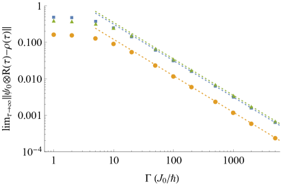
Figure 1: Asymptotic error (Euclidean norm) $\lim_{\tau\to\infty}\|\psi_{0}\otimes R(\tau)-\rho(\tau)\|$ as a function of the dissipation strength $\Gamma$ for the $XYZ$ Heisenberg spin chain with dissipation acting on the first and last spins. Here, $R(\tau)$ is the solution of Eq. (13) whereas $\rho(\tau)$ is the solution of Eq. (1). Parameters: $N=4$, $J_{x}=J_{0},J_{y}=2.2J_{0},J_{z}=0.77J_{0}$ for all data-points. Triangles: $\theta_{L}=\varphi_{L}=\theta_{R}=\varphi_{R}=0$, $\mu_{L}=0.9,\mu_{R}=0.7$. Squares: $\theta_{L}=\pi/3$,$\varphi_{L}=\pi/4$, $\theta_{R}=3\pi/7$, $\varphi_{R}=4\pi/15$, $\mu_{L}=0.9,\mu_{R}=0.7$. Circles: $\theta_{L}=\pi/3$,$\varphi_{L}=\pi/4$, $\theta_{R}=3\pi/7$, $\varphi_{R}=4\pi/15$, $\mu_{L}=0.5,\mu_{R}=-0.3$. The straight lines with slope $1/\Gamma$ are guides to the eye.

IV Heisenberg spin chain with the first and the last spins in a target state

Previous results straightforwardly extend to more general setups. As an example, consider the same spin chain discussed above with dissipation acting only at the boundary spins $1$ and $N$. Within this setup, and by tuning of the Hamiltonian parameters, one can generate, in the Zeno limit, a bulk NESS ranging from a maximally mixed state Popkov et al. (2015) to a pure spin-helix state carrying ballistic current of magnetization Popkov and Presilla (2016); Popkov et al. (2017). Here we assume the dissipation to target generic spin-$1/2$ mixed states, $\psi_{0}^{L}$ and $\psi_{0}^{R}$, at the sites $1$ and $N$, respectively,

$$\psi_{0}^{L} =\frac{1+\mu_{L}}{2}|0_{L}\rangle\langle 0_{L}|+\frac{1-\mu_{L}}{2}|0_{L}^{\perp}\rangle\langle 0_{L}^{\perp}|,$$ (46)

$$\psi_{0}^{R} =\frac{1+\mu_{R}}{2}|0_{R}\rangle\langle 0_{R}|+\frac{1-\mu_{R}}{2}|0_{R}^{\perp}\rangle\langle 0_{R}^{\perp}|.$$ (47)

As discussed above, this is realized by applying two Lindblad operators, of the form (28), at each end of the chain with parameters $\mu_{L}$ and $\mu_{R}$, respectively.

Overall the dissipation targets a state which is the product of the states targeted at the left and right boundaries, $\psi_{0}=\psi_{0}^{L}\otimes\psi_{0}^{R}$. The eigenvalues of the full dissipator are the sum of the eigenvalues of the left and right boundary dissipators separately, $\xi_{m_{L}}+\xi_{m_{R}}$, and the respective eigenvectors are $\psi_{m_{L},m_{R}}=\psi^{L}_{m_{L}}\otimes\psi^{R}_{m_{L}}$, where the individual $\psi^{L,R}_{m}$ have the form (33). The Hamiltonian decomposition in terms of the trace-orthonormal basis for the left and right dissipators, $\varphi^{L}_{n_{L}}$,$\varphi^{R}_{n_{R}}$, now reads

$$H=\sum_{n_{L},n_{R}}\varphi^{L}_{n_{L}}\otimes g_{n_{L},n_{R}}\otimes\varphi^{R}_{n_{R}},$$ (48)

$$g_{n_{L},n_{R}}=\mathop{\mathrm{tr}_{1,N}}\limits[(\psi^{L}_{n_{L}}\otimes I^{2^{N-1}})H(I^{2^{N-1}}\otimes\psi^{R}_{n_{R}})].$$ (49)

We can therefore apply the general formula (24), with $\xi_{m}\to\xi_{m_{L}}+\xi_{m_{R}}$ and $g_{n}\to g_{n_{L},n_{R}}$. Note that, due to the locality of the interactions, $g_{n_{L},n_{R}}=0$ if $n_{L}n_{R}\neq 0$. After some algebra, and using Eq. (23), we obtain that Eq. (24) splits into the sum of two contributions, associated to the left and right ends of the chain,

$$W =\tilde{\mathcal{D}}_{L}R+\tilde{\mathcal{D}}_{R}R,$$ (50)

where, according to (38),

$$\tilde{\mathcal{D}}_{L} =2(1+\mu_{L})\mathcal{D}_{g_{10}}+2(1-\mu_{L})\mathcal{D}_{g_{10}^{\dagger}}+\frac{1}{2}(1-\mu_{L}^{2})\mathcal{D}_{g_{30}},$$

$$\tilde{\mathcal{D}}_{R} =2(1+\mu_{R})\mathcal{D}_{g_{01}}+2(1-\mu_{R})\mathcal{D}_{g_{01}^{\dagger}}+\frac{1}{2}(1-\mu_{R}^{2})\mathcal{D}_{g_{03}}.$$

Also in the present case, $W$ does not have coherent contributions of the kind (26).

The operators $g_{k0},g_{0k}$, as well as the dissipation-projected Hamiltonian $h_{D}$, can be evaluated exactly as in the previous case of a single spin directly affected by the dissipation. The result is expressed in terms of the parameters $\mu_{L},\mu_{R}$ and of the polar coordinates $\theta_{L},\varphi_{L}$ and $\theta_{R},\varphi_{R}$ which define the states $|0_{L}\rangle$ and $|0_{R}\rangle$. In particular, the Hamiltonian $h_{D}$ is again a $XYZ$ Hamiltonian with $M=N-2$ spins, namely, those not directly affected by the dissipation, with two boundary terms relative to the spins 1 and $M$. Explicit formulas will be given elsewhere. In Figs. 1, 2 and 3 we illustrate the behavior of the resulting effective LME in comparison with the exact dynamics of the system.

V Evaluation of the NESS in the Zeno limit

As a direct application of our findings, we can compute the NESS in the Zeno limit, bypassing the solution of the LME. Denote $R_{\infty}=\lim_{\Gamma\rightarrow\infty,\tau\rightarrow\infty}R(\tau)$. From the LME (3) we have

$$[R_{\infty},h_{D}] =0.$$

If the spectrum of the dissipation projected Hamiltonian $h_{D}$ is nondegenerate, then $h_{D}$ and $R_{\infty}$ share the same set of eigenvectors $|\alpha\rangle$. It follows that

$$R_{\infty}=\sum_{\alpha}\nu_{\alpha}^{\infty}|\alpha\rangle\langle\alpha|.$$ (51)

Deriving from (3) an evolution equation for the populations of the eigenstates of $h_{D}$, $\nu_{\alpha}(\tau)=\langle\alpha|R(\tau)|\alpha\rangle$, assuming that the effective dissipator has the canonical form $\mathcal{\tilde{D}}\cdot=\sum_{k}A_{k}({\tilde{L}}_{k}\cdot{\tilde{L}}_{k}^{\dagger}-\frac{1}{2}\{\cdot,{\tilde{L}}_{k}^{\dagger}{\tilde{L}}_{k}\})$ starting from the state $R(\tau)=\sum_{\alpha}\nu_{\alpha}(\tau)|\alpha\rangle\langle\alpha|$, we obtain in the Zeno limit

$$\frac{\partial\nu_{\alpha}(\tau)}{\partial\tau} =\sum_{\beta\neq\alpha}w_{\beta\alpha}\nu_{\beta}-\nu_{\alpha}\sum_{\beta\neq\alpha}w_{\alpha\beta},$$ (52)

$$w_{\beta\alpha} =\frac{1}{\Gamma}\sum_{k}A_{k}\left|\langle\alpha|\tilde{L}_{k}|\beta\rangle\right|^{2}.$$ (53)

We recognize Eq. (52) as the classical master equation of a Markov process with transition rates $w_{\alpha\beta}$. This is a manifestation of the well-known fact that a part of the degrees of freedom of the LME evolves in time via a classical Markov process Breuer and Petruccione (2002); Lesanovsky and Garrahan (2013). Perron-Frobenius theorem guarantees an existence of a time-independent steady state solution of Eq. (52), with non-negative entries $\nu_{\alpha}^{\infty}$. After normalization $\sum_{\alpha}\nu_{\alpha}^{\infty}=1$, the coefficients $\nu_{\alpha}^{\infty}$ acquire the double meaning of eigenvalues of the reduced NESS (51), and steady state probabilities in the associated classical Markov process, see Fig. 2 for an illustration. Note that by diagonalizing $h_{D}$ one gets both the eigenvectors $|\alpha\rangle$ of $R_{\infty}$ and the transition rates $w_{\alpha\beta}$ (and, therefore, the eigenvalues $\nu_{\alpha}^{\infty}$). Thus, the problem of finding the NESS, which generically requires the diagonalization of the full Lindbladian, represented by a non-Hermitian matrix of size $d^{2}\times d^{2}$, reduces, in the Zeno limit, to the diagonalization of the Hermitian matrix $h_{D}$, of size $d_{1}\times d_{1}$ with $d_{1}<d$. In the example discussed in the Sec. IV, we have $d=2^{N}$ and $d_{1}=d/4$.

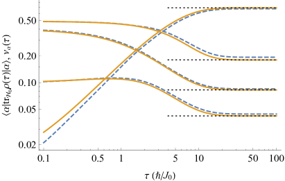
Figure 2: Populations of the eigenstates of $h_{D}$, $\langle\alpha|\mathop{\mathrm{tr}_{\mathcal{H}_{0}}}\limits\rho(\tau)|\alpha\rangle$ (dashed lines) and solutions $\nu_{\alpha}(\tau)$ of the classical Markov equation (52) (solid lines) as a function of time $\tau$ for the $XYZ$ Heisenberg spin chain with dissipation acting on the first and last spins. We set $\Gamma=50J_{0}/\hbar$ and all the other parameters are as in Fig. 1, case of squares. The initial condition is $\rho(0)=\psi_{0}^{L}\otimes R(0)\otimes\psi_{0}^{R}$, where $R(0)$ is a diagonal matrix with entries $0.01,0.4,0.1,0.49$ in the $h_{D}$ basis. The straight dotted lines indicate the exact eigenvalues of $\mathop{\mathrm{tr}_{\mathcal{H}_{0}}}\limits\rho(\tau)$ for $\tau\rightarrow\infty$ in Zeno limit, computed from the Markov process with the rates (53).

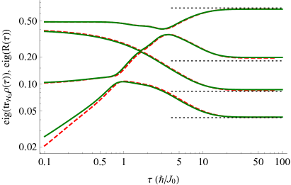
Figure 3: Comparison of the LME and LME effective dynamics: eigenvalues of $\mathop{\mathrm{tr}_{\mathcal{H}_{0}}}\limits\rho(\tau)$ (dashed lines) and of $R(\tau)$ (solid lines) as a function of time $\tau$. Same parameters and same straight dotted lines as in Fig. 2. Note the similarity with Fig. 2 except for the avoided level crossings.

VI Conclusions

One might be concerned that, since our results hold in the Zeno limit, an impractically strong dissipation must be provided. However, one-dimensional quantum many-body systems with dissipation acting on a few degrees of freedom are well suited for an effective Zeno description whenever their size is sufficiently large. To see this fact, consider a one-dimensional system of size $N$ with local interactions and dissipation acting near the edges. Let $\Gamma$ be the finite strength of the dissipation. A perturbation spreads with finite speed (see e.g. Lieb-Robinson bound Lieb and Robinson (1972)), so that the relaxation time of the system toward the global steady state increases at least linearly with the system size, $\tau_{\mathrm{bulk}}\sim N\hbar/J_{0}$, see, e.g., Ref. Žnidarič (2015), while the relaxation of the edges takes a time of the order $\tau_{\mathrm{diss}}\sim 1/\Gamma$. Here, $J_{0}$ is a factor which fixes the energy scale associated to the Hamiltonian of the system. For arbitrary $\Gamma$ and sufficiently large $N$, that is

$$\frac{\hbar\Gamma}{J_{0}}\gg\frac{1}{N},$$ (54)

the system enters an effective Zeno regime $\tau_{\mathrm{diss}}\ll\tau_{\mathrm{bulk}}$, so the NESS of the system should be well approximated by the NESS computed in the Zeno limit $\Gamma\rightarrow\infty$. For a few cases for which exact results are known, validity of the (54) can be demonstrated, see, e.g. Refs. Prosen (2011); Popkov et al. (2013). However if the Zeno NESS is protected by extra symmetries, singular NESS behavior can happen.

Appendix A Proof of Eq. (9)

Here, we compute the Dyson series up to the second order of the perturbation $K$. The calculation follows in part Ref. Zanardi and Campos Venuti (2014) and uses a similar notation.

The time-evolution of the state $\rho=\psi_{0}\otimes R$ is be defined via a Dyson series for $\mathcal{E}(t)\mathcal{P}_{0}$. Up to the second order of the Dyson series, we have

$$\mathcal{E}(t)\mathcal{P}_{0} =e^{\mathcal{L}_{0}t}\left(1+\int_{0}^{t}dt_{1}e^{-\mathcal{L}_{0}t_{1}}Ke^{\mathcal{L}_{0}t_{1}}+\int_{0}^{t}dt_{1}e^{-\mathcal{L}_{0}t_{1}}Ke^{\mathcal{L}_{0}t_{1}}\int_{0}^{t_{1}}dt_{2}e^{-\mathcal{L}_{0}t_{2}}Ke^{\mathcal{L}_{0}t_{2}}+\dots\right)\mathcal{P}_{0}$$

$$=\mathcal{P}_{0}+e^{\mathcal{L}_{0}t}\int_{0}^{t}dt_{1}e^{-\mathcal{L}_{0}t_{1}}Ke^{\mathcal{L}_{0}t_{1}}\mathcal{P}_{0}+e^{\mathcal{L}_{0}t}\int_{0}^{t}dt_{1}e^{-\mathcal{L}_{0}t_{1}}Ke^{\mathcal{L}_{0}t_{1}}\int_{0}^{t_{1}}dt_{2}e^{-\mathcal{L}_{0}t_{2}}Ke^{\mathcal{L}_{0}t_{2}}\mathcal{P}_{0}.$$ (55)

In passing from the first to the second line we have used the obvious relation

$$e^{\mathcal{L}_{0}t}\mathcal{P}_{0}=\mathcal{P}_{0}e^{\mathcal{L}_{0}t}=\mathcal{P}_{0}.$$ (56)

Let us focus on the second term of Eq. (A) and insert the identity decomposition $I=\mathcal{Q}_{0}+\mathcal{P}_{0}$:

$$e^{\mathcal{L}_{0}t}\int_{0}^{t}dt_{1}e^{-\mathcal{L}_{0}t_{1}}Ke^{\mathcal{L}_{0}t_{1}}\mathcal{P}_{0}$$

$$\qquad=e^{\mathcal{L}_{0}t}\int_{0}^{t}dt_{1}e^{-\mathcal{L}_{0}t_{1}}(\mathcal{P}_{0}+\mathcal{Q}_{0})Ke^{\mathcal{L}_{0}t_{1}}\mathcal{P}_{0}$$

$$\qquad=t\mathcal{P}_{0}K\mathcal{P}_{0}+e^{\mathcal{L}_{0}t}\int_{0}^{t}dt_{1}e^{-\mathcal{L}_{0}t_{1}}\mathcal{Q}_{0}K\mathcal{P}_{0}.$$ (57)

In the second term of Eq. (A), we split the integral

$$e^{\mathcal{L}_{0}t}\int_{0}^{t}dt_{1}e^{-\mathcal{L}_{0}t_{1}}\mathcal{Q}_{0}K\mathcal{P}_{0}$$

$$\qquad=e^{\mathcal{L}_{0}t}\left(\int_{0}^{{-\infty}}dt_{1}\dots+\int_{{-\infty}}^{t}dt_{1}\dots\right)$$

$$\qquad=e^{\mathcal{L}_{0}t}\int_{0}^{{-\infty}}dt_{1}e^{-\mathcal{L}_{0}t_{1}}\mathcal{Q}_{0}K\mathcal{P}_{0}$$

$$\qquad\qquad-\int_{t}^{{-\infty}}dt_{1}e^{\mathcal{L}_{0}(t-t_{1})}\mathcal{Q}_{0}K\mathcal{P}_{0},$$ (58)

and, after the substitutions $t_{1}\to-\tilde{t}_{1}$, $dt_{1}\to-d\tilde{t}_{1}$, we obtain

$$e^{\mathcal{L}_{0}t}\int_{0}^{t}dt_{1}e^{-\mathcal{L}_{0}t_{1}}\mathcal{Q}_{0}K\mathcal{P}_{0}$$

$$\qquad=-e^{\mathcal{L}_{0}t}\int_{0}^{{\infty}}d\tilde{t}_{1}e^{\mathcal{L}_{0}\tilde{t}_{1}}\mathcal{Q}_{0}K\mathcal{P}_{0}$$

$$\qquad\qquad+\int_{-t}^{{\infty}}d\tilde{t}_{1}e^{\mathcal{L}_{0}(t+\tilde{t}_{1})}\mathcal{Q}_{0}K\mathcal{P}_{0}.$$ (59)

Next, we make the change of variable $t+\tilde{t}_{1}\rightarrow u$, $d\tilde{t}_{1}\rightarrow du$ in the second integral of Eq. (A) and obtain

$$e^{\mathcal{L}_{0}t}\int_{0}^{t}dt_{1}e^{-\mathcal{L}_{0}t_{1}}\mathcal{Q}_{0}K\mathcal{P}_{0}$$

$$\qquad=-e^{\mathcal{L}_{0}t}\int_{0}^{{\infty}}d\tilde{t}_{1}e^{\mathcal{L}_{0}\tilde{t}_{1}}\mathcal{Q}_{0}K\mathcal{P}_{0}+\int_{0}^{{\infty}}due^{\mathcal{L}_{0}u}\mathcal{Q}_{0}K\mathcal{P}_{0}.$$ (60)

Renaming $\tilde{t}_{1},u\rightarrow t$, we can write

$$e^{\mathcal{L}_{0}t}\int_{0}^{t}dt_{1}e^{-\mathcal{L}_{0}t_{1}}\mathcal{Q}_{0}K\mathcal{P}_{0}=\left(e^{\mathcal{L}_{0}t}-I\right)\mathcal{S}K\mathcal{P}_{0},$$ (61)

where

$$\mathcal{S}=-\int_{0}^{{\infty}}dte^{\mathcal{L}_{0}t}\mathcal{Q}_{0}$$ (62)

is the pseudo-inverse of the dissipator, namely,

$$\mathcal{L}_{0}\mathcal{S}=\mathcal{S}\mathcal{L}_{0}=\mathcal{Q}_{0}.$$ (63)

The operator $\mathcal{S}$ is bounded, since the eigenvalues of $\mathcal{L}_{0}$ (apart from the nondegenerate $0$ eigenvalue which is excluded by the multiplication with $\mathcal{Q}_{0}$) are nonzero and finite. Combining Eqs. (A) and (61), we conclude

$$\mathcal{E}(t)\mathcal{P}_{0} =\mathcal{P}_{0}+t\mathcal{P}_{0}K\mathcal{P}_{0}+\left(e^{\mathcal{L}_{0}t}-I\right)\mathcal{S}K\mathcal{P}_{0}+\ldots$$ (64)

($\ldots$ denoting contributions from second and higher orders), which retrieves the result reported in Ref. [1]. Equation (64) shows, in particular, that the leaking outside the dissipation-free subspace for times $t>1/\Gamma$ is of order $1/\Gamma$, namely,

$$\|\rho(t)-\psi_{0}\otimes\mathop{\mathrm{tr}_{\mathcal{H}_{0}}}\limits\rho(t)\| =O\left(\Gamma^{-1}\right).$$ (65)

The evolution inside the decoherence-free subspace is given by $\mathcal{P}_{0}\mathcal{E}(t)\mathcal{P}_{0}$. Making use of Eq. (56), up to the second order Dyson term we thus obtain

$$\mathcal{P}_{0}\mathcal{E}(t)\mathcal{P}_{0}=\mathcal{P}_{0}+t\mathcal{P}_{0}K\mathcal{P}_{0}+\mathcal{P}_{0}e^{\mathcal{L}_{0}t}$$

$$\qquad\times\int_{0}^{t}dt_{1}e^{-\mathcal{L}_{0}t_{1}}Ke^{\mathcal{L}_{0}t_{1}}\int_{0}^{t_{1}}dt_{2}e^{-\mathcal{L}_{0}t_{2}}Ke^{\mathcal{L}_{0}t_{2}}\mathcal{P}_{0}.$$ (66)

Now we estimate the $O(K^{2})$ contribution to $\mathcal{P}_{0}\mathcal{E}(t)\mathcal{P}_{0}$:

$$\mathcal{P}_{0}e^{\mathcal{L}_{0}t}\int_{0}^{t}dt_{1}e^{-\mathcal{L}_{0}t_{1}}Ke^{\mathcal{L}_{0}t_{1}}\int_{0}^{t_{1}}dt_{2}e^{-\mathcal{L}_{0}t_{2}}Ke^{\mathcal{L}_{0}t_{2}}\mathcal{P}_{0}$$

$$\qquad=\mathcal{P}_{0}\int_{0}^{t}dt_{1}\int_{0}^{t_{1}}dt_{2}Ke^{\mathcal{L}_{0}t_{1}-\mathcal{L}_{0}t_{2}}K\mathcal{P}_{0}$$

$$\qquad=\mathcal{P}_{0}\int_{0}^{t}dt_{1}\int_{0}^{t_{1}}dt_{2}Ke^{\mathcal{L}_{0}t_{1}-\mathcal{L}_{0}t_{2}}(\mathcal{P}_{0}+\mathcal{Q}_{0})K\mathcal{P}_{0}$$

$$\qquad=\frac{t^{2}}{2}(\mathcal{P}_{0}K\mathcal{P}_{0})^{2}$$

$$\qquad\qquad+\mathcal{P}_{0}K\int_{0}^{t}dt_{1}e^{\mathcal{L}_{0}t_{1}}\int_{0}^{t_{1}}dt_{2}e^{-\mathcal{L}_{0}t_{2}}\mathcal{Q}_{0}K\mathcal{P}_{0}$$

$$\qquad=\frac{t^{2}}{2}(\mathcal{P}_{0}K\mathcal{P}_{0})^{2}+\mathcal{P}_{0}K\int_{0}^{t}dt_{1}\left(e^{\mathcal{L}_{0}t}-I\right)\mathcal{S}K\mathcal{P}_{0}$$

$$\qquad=\frac{t^{2}}{2}(\mathcal{P}_{0}K\mathcal{P}_{0})^{2}-t\mathcal{P}_{0}K(\mathcal{P}_{0}+\mathcal{Q}_{0})\mathcal{S}K\mathcal{P}_{0}$$

$$\qquad\qquad+\mathcal{P}_{0}K\int_{0}^{t}dt_{1}e^{\mathcal{L}_{0}t}\mathcal{S}K\mathcal{P}_{0}.$$ (67)

Let us concentrate on the last term of the above expression. Inserting the identity decomposition $I=\mathcal{Q}_{0}+\mathcal{P}_{0}$ and using Eq. (56), we have

$$\mathcal{P}_{0}K\int_{0}^{t}dt_{1}e^{\mathcal{L}_{0}t}\mathcal{S}K\mathcal{P}_{0}$$

$$\qquad=\mathcal{P}_{0}K\int_{0}^{t}dt_{1}e^{\mathcal{L}_{0}t}(\mathcal{P}_{0}+\mathcal{Q}_{0})\mathcal{S}K\mathcal{P}_{0}$$

$$\qquad=t\mathcal{P}_{0}K\mathcal{P}_{0}\mathcal{S}K\mathcal{P}_{0}+\mathcal{P}_{0}K\int_{0}^{t}dt_{1}e^{\mathcal{L}_{0}t}\mathcal{Q}_{0}\mathcal{S}K\mathcal{P}_{0}.$$ (68)

Gathering all terms of order $K^{2}$, we conclude

$$\mathcal{P}_{0}e^{\mathcal{L}_{0}t}\int_{0}^{t}dt_{1}e^{-\mathcal{L}_{0}t_{1}}Ke^{\mathcal{L}_{0}t_{1}}\int_{0}^{t_{1}}dt_{2}e^{-\mathcal{L}_{0}t_{2}}Ke^{\mathcal{L}_{0}t_{2}}\mathcal{P}_{0}$$

$$\qquad=\frac{t^{2}}{2}(\mathcal{P}_{0}K\mathcal{P}_{0})^{2}-t\mathcal{P}_{0}K\mathcal{Q}_{0}\mathcal{S}K\mathcal{P}_{0}$$

$$\qquad\qquad+\mathcal{P}_{0}K\int_{0}^{t}dt_{1}e^{\mathcal{L}_{0}t}\mathcal{Q}_{0}\mathcal{S}K\mathcal{P}_{0}.$$ (69)

In the last term of Eq. (69), the integral over time converges, thus this term is of order $\|K^{2}\|=O(1/\Gamma^{2})$ and can be neglected. Bringing together Eqs. (66) and (69), we obtain Eq. (9).

References

• Lindblad (1976) G. Lindblad, “On the generators of quantum dynamical semigroups,” Communications in Mathematical Physics 48, 119–130 (1976).
• Gorini et al. (1976) V. Gorini, A. Kossakowski,  and E. C. G. Sudarshan, “Completely positive dynamical semigroups of $N$-level systems,” Journal of Mathematical Physics 17, 821–825 (1976).
• Breuer and Petruccione (2002) H.-P. Breuer and F. Petruccione, The Theory of Open Quantum Systems (Oxford University Press, Oxford, 2002).
• Clark et al. (2010) S. R. Clark, J. Prior, M. J. Hartmann, D. Jaksch,  and M. B. Plenio, “Exact matrix product solutions in the Heisenberg picture of an open quantum spin chain,” New Journal of Physics 12, 025005 (2010).
• Misra and Sudarshan (1977) B. Misra and E. C. G. Sudarshan, “The Zeno’s paradox in quantum theory,” Journal of Mathematical Physics 18, 756–763 (1977).
• Koshino and Shimizu (2005) K. Koshino and A. Shimizu, “Quantum zeno effect by general measurements,” Physics Reports 412, 191 – 275 (2005).
• Itano et al. (1990) W. M. Itano, D. J. Heinzen, J. J. Bollinger,  and D. J. Wineland, “Quantum zeno effect,” Phys. Rev. A 41, 2295–2300 (1990).
• Kwiat et al. (1995) P. Kwiat, H. Weinfurter, T. Herzog, A. Zeilinger,  and M. A. Kasevich, “Interaction-free measurement,” Phys. Rev. Lett. 74, 4763–4766 (1995).
• Signoles et al. (2014) A. Signoles, A. Facon, D. Grosso, I. Dotsenko, S. Haroche, J.-M. Raimond, M. Brune,  and S. Gleyzes, “Confined quantum Zeno dynamics of a watched atomic arrow,” Nature Physics 10, 715–719 (2014).
• Schäfer et al. (2014) F. Schäfer, I. Herrera, S. Cherukattil, C. Lovecchio, F. S. Cataliotti, F. Caruso,  and A. Smerzi, “Experimental realization of quantum Zeno dynamics,” Nature Communications 5, 1–6 (2014).
• Patil et al. (2015) Y. S. Patil, S. Chakram,  and M. Vengalattore, “Measurement-induced localization of an ultracold lattice gas,” Phys. Rev. Lett. 115, 140402 (2015).
• Beige et al. (2000) A. Beige, D. Braun, B. Tregenna,  and P. L. Knight, “Quantum computing using dissipation to remain in a decoherence-free subspace,” Phys. Rev. Lett. 85, 1762–1765 (2000).
• Verstraete et al. (2009) F. Verstraete, M. M. Wolf,  and J. Ignacio Cirac, “Quantum computation and quantum-state engineering driven by dissipation,” Nature Physics 5, 633–636 (2009).
• Yi et al. (2012) W. Yi, S. Diehl, A. J. Daley,  and P. Zoller, “Driven-dissipative many-body pairing states for cold fermionic atoms in an optical lattice,” New Journal of Physics 14, 055002 (2012).
• Elliott et al. (2015) T. J. Elliott, W. Kozlowski, S. F. Caballero-Benitez,  and I. B. Mekhov, “Multipartite entangled spatial modes of ultracold atoms generated and controlled by quantum measurement,” Phys. Rev. Lett. 114, 113604 (2015).
• Winkler et al. (2006) K. Winkler, G. Thalhammer, F. Lang, R. Grimm, J. Hecker Denschlag, A. J. Daley, A. Kantian, H. P. Büchler,  and P. Zoller, “Repulsively bound atom pairs in an optical lattice,” Nature (London) 441, 853–856 (2006).
• Stannigel et al. (2014) K. Stannigel, P. Hauke, D. Marcos, M. Hafezi, S. Diehl, M. Dalmonte,  and P. Zoller, “Constrained dynamics via the zeno effect in quantum simulation: Implementing non-abelian lattice gauge theories with cold atoms,” Phys. Rev. Lett. 112, 120406 (2014).
• Ashida and Ueda (2015) Y. Ashida and M. Ueda, “Diffraction-unlimited position measurement of ultracold atoms in an optical lattice,” Phys. Rev. Lett. 115, 095301 (2015).
• Lee and Ruostekoski (2014) M. D. Lee and J. Ruostekoski, “Classical stochastic measurement trajectories: Bosonic atomic gases in an optical cavity and quantum measurement backaction,” Phys. Rev. A 90, 023628 (2014).
• Elliott and Mekhov (2016) T. J. Elliott and I. B. Mekhov, “Engineering many-body dynamics with quantum light potentials and measurements,” Phys. Rev. A 94, 013614 (2016).
• Ashida and Ueda (2017) Y. Ashida and M. Ueda, “Multiparticle quantum dynamics under real-time observation,” Phys. Rev. A 95, 022124 (2017).
• Kozlowski et al. (2016) W. Kozlowski, S. F. Caballero-Benitez,  and I. B. Mekhov, “Non-hermitian dynamics in the quantum zeno limit,” Phys. Rev. A 94, 012123 (2016).
• Elliott and Vedral (2016) T. J. Elliott and V. Vedral, “Quantum quasi-zeno dynamics: Transitions mediated by frequent projective measurements near the zeno regime,” Phys. Rev. A 94, 012118 (2016).
• Zanardi and Campos Venuti (2014) P. Zanardi and L. Campos Venuti, “Coherent quantum dynamics in steady-state manifolds of strongly dissipative systems,” Phys. Rev. Lett. 113, 240406 (2014).
• Carollo et al. (2006) A. Carollo, M. F. Santos,  and V. Vedral, “Coherent quantum evolution via reservoir driven holonomies,” Phys. Rev. Lett. 96, 020403 (2006).
• Prosen (2011) T. Prosen, “Exact nonequilibrium steady state of a strongly driven open XXZ chain,” Phys. Rev. Lett. 107, 137201 (2011).
• Popkov et al. (2015) V. Popkov, M. Salerno,  and R. Livi, “Full decoherence induced by local fields in open spin chains with strong boundary couplings,” New Journal of Physics 17, 023066 (2015).
• Popkov and Presilla (2016) V. Popkov and C. Presilla, “Obtaining pure steady states in nonequilibrium quantum systems with strong dissipative couplings,” Phys. Rev. A 93, 022111 (2016).
• Popkov et al. (2017) V. Popkov, C. Presilla,  and J. Schmidt, “Targeting pure quantum states by strong noncommutative dissipation,” Phys. Rev. A 95, 052131 (2017).
• Lesanovsky and Garrahan (2013) I. Lesanovsky and J. P. Garrahan, “Kinetic constraints, hierarchical relaxation, and onset of glassiness in strongly interacting and dissipative rydberg gases,” Phys. Rev. Lett. 111, 215305 (2013).
• Lieb and Robinson (1972) E. H. Lieb and D. W. Robinson, “The finite group velocity of quantum spin systems,” Comm. Math. Phys. 28, 251–257 (1972).
• Žnidarič (2015) M. Žnidarič, “Relaxation times of dissipative many-body quantum systems,” Phys. Rev. E 92, 042143 (2015).
• Popkov et al. (2013) V. Popkov, D. Karevski,  and G. M. Schütz, “Driven isotropic heisenberg spin chain with arbitrary boundary twisting angle: Exact results,” Phys. Rev. E 88, 062118 (2013).