Temporal disorder in discontinuous non-equilibrium phase transitions: general results

Abstract

We develop a general theory for discontinuous non-equilibrium phase transitions into an absorbing state in the presence of temporal disorder. We focus in two paradigmatic models for discontinuous transitions: the quadratic contact process (in which activation is only spread when two nearest-neighbor sites are both active) and the contact process with long-range interactions. Using simple stability arguments (supported by Monte Carlo simulations), we show that temporal disorder does not destroy the discontinuous transition in the former model. For the latter one, the first-order transition is turned into a continuous one only in the strong-disorder limit, with critical behavior belonging to the infinite-noise universality class of the contact process model. Finally, we have found that rare temporal fluctuations dramatically changes the behavior of metastable phase turning it into a temporal Griffiths inactive phase characterized by an exponentially large decay time.

I Introduction

Non-equilibrium phase transitions have constituted a rich and lively topic of research for many years. They occur in a wide variety of models in ecology Kussell and Vucelja (2014), epidemic spreading Pastor-Satorras et al. (2015), sociophysics Sen and Chakrabarti (2013), catalytic reactions Ziff et al. (1986), depinning interface growth Tang and Leschhorn (1992); Buldyrev et al. (1992), turbulent flow Pomeau (1986), among other fields Marro and Dickman (1999); Henkel et al. (2008); Ódor (2004).

Since disorder due to spatial or temporal inhomogeneities is almost an unavoidable ingredient in many real systems, it is then desirable to understand their effects on these phase transitions. For continuous phase transitions, it was earlier recognized that spatial and temporal disorder changes the critical behavior whenever the generalized Harris criterion is violated Kinzel (1985); Noest (1986): quenched spatial disorder is relevant whenever $d\nu_{\perp}>2$ is violated while temporal disorder is relevant when $\nu_{\parallel}=z\nu_{\perp}>2$ is violated; with $\nu_{\perp},$ $\nu_{\parallel}$ and $z$ being critical exponents of the clean phase transition and $d$ being the number of spatial dimensions. Since the critical exponents of the directed percolation universality class violate the Harris criterion, it was then argued that this was the reason why it was never seen in experiments Hinrichsen (2000) (see however Ref. Takeuchi et al., 2007).

Later, it was shown that spatial disorder yields a critical behavior in the exotic universality class of infinite-randomness type surrounding accompanied by a Griffiths effects in the inactive phase Hooyberghs et al. (2003); Vojta and Dickison (2005); Vojta and Lee (2006); Hoyos (2008); de Oliveira and Ferreira (2008); Vojta et al. (2009). More recently, it was shown that temporal disorder yields to analogous effects, namely, an exotic infinite-noise universality class accompanied by a temporal Griffiths active phase Vazquez et al. (2011); Vojta and Hoyos (2015); Barghathi et al. (2016); Solano et al. (2016).

The effects of disorder in discontinuous non-equilibrium phase transitions are much less understood. It was initially shown that quenched spatial disorder can turn a discontinuous transition into a continuous one Hoenicke and Figueiredo (2000) and later, it was argued that it actually prohibits phase coexistence and discontinuous transitions in $d\leq 2$ Villa Martín et al. (2014). In the case of temporal disorder, however, a recent numerical study indicates that first-order phase transitions can happen in low-dimensional systems de Oliveira and Fiore (2016).

In this work, we develop a general theory for discontinuous non-equilibrium phase transition in the presence of temporal disorder. Analysis of two paradigmatic models in mean-field level is sufficient to draw quantitative accurate predictions which we confirm in $d=1$ and $2$ via Monte Carlo simulations. Our main result is that temporal disorder does not forbid first-order phase transitions. In addition, it can also turn a discontinuous transition into a continuous one when disorder is sufficiently strong. Furthermore, we find an interesting novel phenomena: temporal disorder turns the clean metastable active phase into a temporal Griffiths inactive phase characterized by extremely large decay times.

The remainder of this article, we define the studied models in Sec. II, develop our main theory in Sec. III where a mean-field analysis is performed. In Sec. IV we provide Monte Carlo simulations confirming our theory and leave concluding remarks to Sec. A.

II The models

The usual contact process (CP) model Harris (1974); Marro and Dickman (1999) is defined on a $d$-dimensional lattice in which each site is either active ($A$) or inactive ($I$). The corresponding dynamics has the following processes: (i) a spontaneous inactivation and (ii) an autocatalytic activation via nearest-neighbor contact. In the former, a single active site spontaneously decays to the inactive state with rate $\mu$. In the latter, an active site turns an inactive nearest-neighbor site into an active one with rate $\lambda$. Schematically, $A\stackrel{{\scriptstyle\mu}}{{\rightarrow}}I$ and $A+I\stackrel{{\scriptstyle\lambda}}{{\rightarrow}}2A$, respectively.

In this work, we study a particular case of the second Schlögl model Schlögl (1972), known as the quadratic contact process (QCP) model and a version of the CP model with long-range interactions known as the $\sigma$CP model Ginelli et al. (2005). They are identical to the CP model except for the activity spreading dynamics. In the QCP model, activity is spread via the contact with two active nearest-neighbor sites: $2A+I\stackrel{{\scriptstyle\lambda}}{{\rightarrow}}3A$. In the $\sigma$CP model, the activation rate depends on the length $\ell$ of the continuous string of inactive sites between two active ones, i.e., $\lambda\rightarrow\lambda_{\ell}=\lambda\left(1+a\ell^{-\sigma}\right)$, where $a\geq 0$ and $\sigma>0$ are constants controlling the long-range “interaction” (with $a=0$ recovering the CP model). Schematically, the reaction is $A+I^{\ell}\stackrel{{\scriptstyle\lambda_{\ell}}}{{\rightarrow}}2A+I^{\ell-1}$, where $I^{\ell}$ denotes the continuous string of $\ell$ inactive sites.

For simplicity, we set $\mu+\lambda=1$ and only deals with $\lambda\in[0,1]$.

Noise fluctuations (temporal disorder) are introduced in these models by considering $\lambda$ as a random time-dependent variable. For concreteness, we divide the system time evolution in time intervals of equal duration $\Delta t$ within which $\lambda$ is constant, i.e., over the $i$-th time interval the activity spreading rate equals $\lambda=\lambda_{i}$, with $\lambda_{i}$ being an independent random variable drawn from a binary probability density distribution

$$P(\lambda)=p\delta(\lambda-\lambda_{-})+\left(1-p\right)\delta(\lambda-\lambda_{+}),$$ (1)

with $\lambda_{+}>\lambda_{-}$. For later convenience, we rewrite $\lambda_{\pm}$ in terms of the average $\overline{\lambda}=p\lambda_{-}+\left(1-p\right)\lambda_{+}$ and $\delta\lambda=\lambda_{+}-\lambda_{-}$ (which represents the disorder strength), namely, $\lambda_{+}=\overline{\lambda}+p\delta\lambda$ and $\lambda_{-}=\overline{\lambda}-\left(1-p\right)\delta\lambda$. We report that we have also considered box-like distributions and have found no qualitative difference.

III The mean-field approach

In this Section, we present our mean-field approach for the effects of temporal disorder on the first-order non-equilibrium phase transitions to an absorbing state.

III.1 The clean system

We start by reviewing some key aspects of the clean phase transition and later consider the effects of temporal disorder.

III.1.1 Mean-field approach for the clean QCP model

Let us start with the QCP model at the level of one-site mean-field theory. The density of active sites $\rho$ obeys the following logistic equation

$$\frac{{\rm d}\rho}{{\rm d}t}=-(1-\lambda)\rho+\lambda\rho^{2}(1-\rho),$$ (2)

where the first term on the RHS accounts for the spontaneous inactivation processes, whereas the second one corresponds to the activity spreading.

There are three steady-state (time-independent) solutions $\rho_{\infty}$ for Eq. (2):

$$\rho_{\infty}^{(I)}=0,\mbox{ }\rho_{\infty}^{(S)}=\frac{1}{2}+\alpha,\mbox{ and }\rho_{\infty}^{(U)}=\frac{1}{2}-\alpha,$$ (3)

with $\alpha=\sqrt{\frac{5}{4}-\frac{1}{\lambda}}$. A phase transition occurs at $\lambda=\lambda_{c}=\frac{4}{5}$ above which $\rho_{\infty}^{(S)}$ and $\rho_{\infty}^{(U)}$ exist ($\alpha\in\mathbb{R}$). As $\rho_{\infty}^{(S,U)}\rightarrow\frac{1}{2}$ when $\lambda\rightarrow\lambda_{c}^{+}$, notice the transition is discontinuous with the order parameter being $\rho_{c}=\frac{1}{2}$ at the transition. In order to better understand the phases surrounding the transition point, we study the stability of the steady-state solutions $\rho_{\infty}$ by linearizing Eq. (2). It is found that $\rho_{\infty}^{(I)}$ is a stable solution for $0\leq\lambda<\lambda^{*}=1$ with small deviations from it ($r=\rho-\rho_{\infty}$) vanishing exponentially $r\sim e^{-\left(1-\lambda\right)t}$ for large $t$. Likewise, $\rho_{\infty}^{(S)}$ is a stable solution (for $\lambda>\lambda_{c}$) with small deviations vanishing as $\left|r\right|\sim e^{-\left[\left(\frac{5}{2}+\alpha\right)\lambda-2\right]t}$ for large $t$. Finally, the $\rho_{\infty}^{(U)}$ is an unstable solution (for $\lambda>\lambda_{c}$) in which deviations grow as $\left|r\right|\sim e^{\left[2-\left(\frac{5}{2}-\alpha\right)\lambda\right]t}$ for small $t$. At the transition point $\lambda=\lambda_{c}$, the solutions $\rho_{\infty}^{(S,U)}$ degenerate and become a saddle point. In this case when $\rho>\rho_{c}=\rho_{\infty}^{(S,U)}$, the deviations vanish algebraically as $r\sim t^{-1}$ for large $t$, otherwise when $\rho<\rho_{c}$, they increase as $r\approx-\left|r_{0}\right|(1+\left|r_{0}\right|\rho_{c}\lambda_{c}t)$ for small $t$.

We call attention to the fact that for $\lambda_{c}\leq\lambda<\lambda^{*}$ there are two stable solutions $\rho_{\infty}^{(I,S)}$ being one of them corresponding to the inactive absorbing state. As we show latter, this bistability is an important feature for understanding the temporal disorder effects. For this reason, we refer to this region of the active phase as metastable phase.

Figure 1: Mean-field phase diagram of the clean (a) QCP and (b) $\sigma$CP models (see main text). The dashed line denotes a first-order phase transition and the solid line denotes a second order one belonging to the directed percolation universality class. The dotted line denotes the end of the bistability in the active phase. For the QCP model, $\lambda_{c}=\frac{4}{5}$. For the $\sigma$CP model, $\lambda^{*}=\frac{1}{2}$.

The mean-field phase diagram of the QCP model is shown in Fig. 1(a). For $0\leq\lambda<\lambda_{c}$, the system is in the inactive phase in which any activity becomes extinct as $t\rightarrow\infty$ with $\rho\rightarrow\rho_{\infty}^{(I)}$. For $\lambda_{c}<\lambda<1$, the system is in the metastable phase in which activity persists ($\rho\rightarrow\rho_{\infty}^{(S)}$) indefinitely if the initial density $\rho(0)\equiv\rho_{0}$ is greater than $\rho_{\infty}^{(U)}$, otherwise the system evolves towards the absorbing state. The transition at $\lambda=\lambda_{c}$ between the inactive and the metastable phase is discontinuous. Finally, at $\lambda=\lambda^{*}=1$ the system is in the usual active phase.

It worth noting that Eq. (2) can be fully integrated, yielding

$$\ln\left(\frac{\rho}{\rho_{0}}\right)-\left(\frac{\rho_{\infty}^{(S)}}{2\alpha}\right)\ln\left(\frac{\rho-\rho_{\infty}^{(U)}}{\rho_{0}-\rho_{\infty}^{(U)}}\right)$$

$$+\left(\frac{\rho_{\infty}^{(U)}}{2\alpha}\right)\ln\left(\frac{\rho-\rho_{\infty}^{(S)}}{\rho_{0}-\rho_{\infty}^{(S)}}\right) =-\left(1-\lambda\right)t.$$ (4)

From this solution, all previous conclusions follow straightforwardly. Evidently, at the transition point $\lambda=\lambda_{c}$, a direct integration of the resulting logistic equation $\frac{{\rm d}\rho}{{\rm d}t}=-\lambda_{c}\rho(\rho-\rho_{c})^{2}$ yields to

$$\ln\left(\frac{\rho_{0}\left(\rho-\rho_{c}\right)}{\rho\left(\rho_{0}-\rho_{c}\right)}\right)+\frac{\rho_{c}\left(\rho_{0}-\rho\right)}{\left(\rho-\rho_{c}\right)\left(\rho_{0}-\rho_{c}\right)}=\rho_{c}^{2}\lambda_{c}t.$$ (5)

Decay time towards the absorbing state close to the transition: general results

An important quantity for our analysis is the time $T$ necessary for the system to decay into the absorbing state when it is in the inactive phase but very close to the transition, i.e., when $\lambda=\lambda_{c}-\ell$, with $0<\ell\ll\lambda_{c}$ (see Fig. 2). A intuitive definition for $T$ would be the following: starting from $\rho_{0}=1,$ the decay time $T$ is such that$\rho(T)\ll\rho_{c}$. Although this can be easily accomplished, we adopt another (and more elegant) one: We define $T$ as the time interval for the evolution from $\rho_{0}=\rho_{c}+\epsilon$ to $\rho(T)=\rho_{c}-\epsilon$, with $0<\epsilon\ll\rho_{c}$. Since we now have to small parameters $\frac{\ell}{\lambda_{c}}$ and $\frac{\epsilon}{\rho_{c}}$, we now need to specify which one is smaller. Since we wish to connect with the first definition, we then require that $\frac{\ell}{\lambda_{c}}\lll\frac{\epsilon}{\rho_{c}}$. Inspections o the resulting logistic equation show that $\ell\rho_{c}^{2}\ll\epsilon^{2}\lambda_{c}$ is sufficient.

We are now in position of computing $T$. This task can accomplish in more general grounds (applicable to other models) by considering a logistic equation of type

$$\frac{{\rm d}\rho}{{\rm d}t}=\rho\left(\lambda f(\rho)-1\right).$$ (6)

(The choice $f=1+\rho-\rho^{2}$ recovers the QCP model.) The discontinuous transition point $\lambda_{c}$ and density $\rho_{c}$ are obtained from $\lambda_{c}f(\rho_{c})=1$ and $f^{\prime}(\rho_{c})=0$. Defining $\rho(t)=\rho_{c}-r(t)$, we study the time $T$ required for $r(t)$ evolving from $-\epsilon$ to $\epsilon$. Expanding the logistic equation (6) for $\left|r\right|$ and $\ell$ (and noticing that $f^{\prime\prime}(\rho_{c})<0$), then

$$\frac{\text{d}r}{r^{2}+R^{2}}\approx\frac{\pi}{RT}\text{d}t,$$ (7)

where $R=\sqrt{\frac{2\ell}{\left|f^{\prime\prime}(\rho_{c})\right|}}f(\rho_{c})$ and

$$T=\frac{2\pi}{\sqrt{2\ell\left|f^{\prime\prime}(\rho_{c})\right|}\rho_{c}}=t_{0}\left(\lambda_{c}-\lambda\right)^{-\phi}.$$ (8)

The time scale $T$ is exactly the decay time obtained by integrating Eq. (7) from $-\epsilon$ to $\epsilon$ and taking the limit $\epsilon\gg R$. We finally conclude that, in the mean-field approximation, $T$ diverges with exponent $\phi=\frac{1}{2}$. (For the QCP model, the microscopic time scale is $t_{0}=2\pi$, see also Fig. (2)).

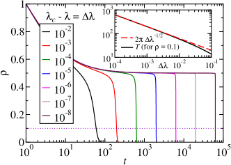
Figure 2: The mean-field density $\rho$ as a function of time $t$ for the QCP model for various activation rates $\lambda$ in the inactive phase $\lambda<\lambda_{c}$. The inset shows the time $T$ when $\rho=0.1$ (dotted line of the main panel). The dashed line is the analytical result Eq. (8).

III.1.2 Mean-field approach for the clean $\sigma$CP model

In this case, at the level of one-site mean-field theory, the density of active sites $\rho$ is obtained from

$$\frac{{\rm d}\rho}{{\rm d}t} =-(1-\lambda)\rho+\lambda\rho^{2}\sum_{{\rm\ell=1}}^{\infty}(1+a\ell^{-\sigma})(1-\rho)^{\ell}$$

$$=(2\lambda-1)\rho-\lambda\rho^{2}\left[1-ag_{\sigma}(1-\rho)\right],$$ (9)

where $g_{\nu}(z)=\sum_{\ell=1}^{\infty}\frac{z^{\ell}}{\ell^{\nu}}=\frac{1}{\Gamma(\nu)}\int_{0}^{\infty}\frac{x^{\nu-1}}{z^{-1}e^{x}-1}{\rm d}x$ is the Polylogarithm function which, for $0\leq z<1$ and $\nu>0$, becomes the familiar Bose-Einstein function. Notice that when $ag_{\sigma}\left(1-\rho\right)\geq 1$, the nonlinear term $\propto\rho^{2}$ changes sign and a new behavior is expected, otherwise the same physics of the usual CP model is recovered. Finally, notice that Eq. (9) is of the type (6) with $f=2-\rho\left(1-ag_{\sigma}\left(1-\rho\right)\right)$.

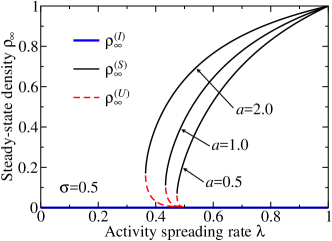
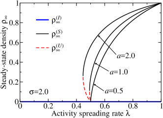
Figure 3: The possible steady-state densities $\rho_{\infty}$ as a function of the activity spreading rate $\lambda$ for the values of the exponent $\sigma=0.5$ (top) and $\sigma=2.0$ (bottom panel) and various values of the parameter $a$ as indicated.

As in the QCP model, there is a trivial steady-state density $\rho_{\infty}^{(I)}=0$ representing the inactive absorbing state. It is stable for $\lambda\leq\lambda^{*}=\frac{1}{2}$ and unstable for $\lambda>\lambda^{*}$. Thus, $\lambda>\lambda^{*}$ delimits the usual active phase (without bistability). Nontrivial steady-state densities are shown in Fig. 3 for some values of $a$ and $\sigma$, which are the real solutions of the equation $f(\rho_{\infty})=\lambda^{-1}$, namely

$$\rho_{\infty}\left[1-ag_{\sigma}(1-\rho_{\infty})\right]=2-\lambda^{-1}.$$ (10)

When $\lambda>\lambda^{*}$, Eq. (10) has only one stable solution $\rho_{\infty}^{(S)}$ corresponding to the usual active phase as already anticipated. When $f^{\prime}\left(0\right)>0$ (or $ag_{\sigma}(1)>1$), Eq. (10) has two finite-density steady-state solutions: $\rho_{\infty}^{(S)}$ and $\rho_{\infty}^{(U)}$ (with $\rho_{\infty}^{(S)}\geq\rho_{\infty}^{(U)}$) which are stable and unstable, respectively. Thus, the region $\lambda_{c}<\lambda<\lambda^{*}$ corresponds to the metastable phase. At $\lambda=\lambda^{*}$, the bistability of the active phase ends.

For $f^{\prime}(0)>0,$ it is clear the transition from the inactive phase to a metastable phase at $\lambda=\lambda_{c}<\lambda^{*}$ is discontinuous. The order parameter $\rho_{c}$ at the discontinuous transition is obtained from $f^{\prime}(\rho_{c})=0$, i.e., $a^{-1}=g_{\sigma}(1-\rho_{c})-\frac{\rho_{c}}{1-\rho_{c}}g_{\sigma-1}(1-\rho_{c})$. The corresponding transition point is $\lambda_{c}=f^{-1}(\rho_{c})=[2-\rho_{c}(1-ag_{\sigma}(1-\rho_{c}))]^{-1}$ [see the dashed line in Fig. 1(b)]. On the other hand if $ag_{\sigma}\left(1\right)\leq 1$, the transition from the inactive to the active phase is continuous at $\lambda=\lambda^{*}$ and belonging to the directed percolation universality class.

Finally, at the inactive phase but near the transition point to the metastable phase, $\lambda=\lambda_{c}-\ell$, the time needed for decay from an initial state such that $\rho(0)>\rho_{c}$ diverges when $\ell\rightarrow 0^{+}$ as $T=t_{0}\ell^{-\phi}$, with exponent $\phi=\frac{1}{2}$ and constant $t_{0}=2\pi\left(\rho_{c}^{-1}-1\right)/\sqrt{2a\left[\left(2-\rho_{c}\right)g_{\sigma-1}-\rho_{c}g_{\sigma-2}\right]}$, according to Eq. (8).

III.2 Overview of the temporal disorder effects

Let us now discuss the effects of temporal disorder on the clean phase diagram of the QCP and $\sigma$CP models (see Fig. 1). For simplicity, we assume that $\lambda$ takes only two possible distinct values with equal and independent probabilities [see Eq. (1) for $p=1/2$] along system time evolution. As will become clear, although we base our quantitative conclusions on the mean-field analysis, our conclusions are qualitatively applicable to any dimension provided that it supports a discontinuous phase transition.

III.2.1 Effects on the phases

Firstly, let us discuss the effects of temporal disorder on the nature of the phases, i.e., let us discuss the case in which both $\lambda_{-}$ and $\lambda_{+}$ are in the same (clean) phase.

When $0\leq\lambda_{\pm}<\lambda_{c}$, the system inevitably evolves into the absorbing state, and hence, the inactive phase is not qualitatively affected by the temporal disorder. Naturally, the decay dynamics change whether $\lambda=\lambda_{+}$ or $\lambda_{-}$.

Likewise, the active phase is also unaffected by disorder ($\lambda^{*}<\lambda_{\pm}\leq 1$). Evidently, the steady-state density $\rho_{\infty}$ fluctuates between the corresponding values $\rho_{\infty}^{(S)}(\lambda_{-})$ and $\rho_{\infty}^{(S)}(\lambda_{+})$, but the main feature of supporting long-standing activity regardless of the initial state (provided that $\rho_{0}\neq 0$) is unaffected.

The analysis of the metastable phase is more involving. Since $\rho_{\infty}^{(U)}(\lambda_{+})<\rho_{\infty}^{(U)}(\lambda_{-})$ [see, e.g., Eq. (3) and Fig. 3], when the initial state density $\rho_{0}\geq\rho_{\infty}^{(U)}(\lambda_{-})$ [$\rho_{0}\leq\rho_{\infty}^{(U)}(\lambda_{+})$], the system will evolve to the active [inactive] state just like in the clean metastable phase. The new feature happens when $\rho_{\infty}^{(U)}(\lambda_{+})<\rho_{0}<\rho_{\infty}^{(U)}(\lambda_{-})$. In this case, the fate of the density will depend on the details of the temporal fluctuation. If a rare fluctuation of long activity window appears in the beginning, i.e., if initially $\lambda=\lambda_{+}$ for a sufficiently long period, the density then increases beyond $\rho_{\infty}^{(U)}(\lambda_{-})$ and the system will thus evolve towards the long-standing activity. On the other hand if this rare fluctuation is such that$\lambda=\lambda_{-}$, then $\rho$ will become less than $\rho_{\infty}^{(U)}(\lambda_{+})$ putting the system towards inactivity. The lack of determinism for the evolution of $\rho(t)$ based only on knowledge of the initial condition $\rho_{0}$ is a new feature appearing in the metastable phase due to temporal disorder in the region $\rho_{\infty}^{(U)}(\lambda_{+})<\rho_{0}<\rho_{\infty}^{(U)}(\lambda_{-})$.

III.2.2 Effects on the phase transitions

Let us now discuss the more interesting cases when $\lambda_{-}$ and $\lambda_{+}$ are in different phases of the clean phase diagram. We start analyzing the case when there is a mix of the inactive ($\lambda_{-}<\lambda_{c}$) and the metastable ($\lambda_{c}\leq\lambda_{+}<\lambda^{*}$) phases. Here, temporal disorder destroys the metastable phase replacing it by the inactive one. The explanation is simple. After a sufficiently long time, the system encounters with probability one a rare fluctuation in which $\lambda=\lambda_{-}$ for a sufficiently long time interval [greater than $T$ in Eq. (8)]. When this happens, $\rho$ evolves below $\rho_{\infty}^{(U)}(\lambda_{+})$ and thus, the system activity decays towards extinction. In addition, notice that the first-order character of the transition between the inactive and metastable phase (happening when $\lambda_{-}\rightarrow\lambda_{c}$) is preserved.

Because extinction happens only after a large and rare temporal interval in the inactive phase, we call this phase as temporal Griffiths inactive phase. Evidently, confirming the complete destruction of the metastable phase numerically is a difficult task since the time $T^{\prime}$ needed for $\rho$ evolving below $\rho_{\infty}^{(U)}(\lambda_{+})$ is exponentially large in the interesting regime of $\lambda_{-}$ being sufficiently close to $\lambda_{c}$ (or $\Delta t\ll T$) and $\lambda_{+}$ being far from $\lambda_{c}$. On average, the upper limit time for decaying into the absorbing state is given by (see Appendix (A))

$$\ln\overline{T^{\prime}}\sim-\frac{\ln p}{\Delta t\left(\lambda_{c}-\lambda_{-}\right)^{\phi}},$$ (11)

with $p$ and $\Delta t$ defined in Eq. (1) and the diverging $T\sim\left(\lambda_{c}-\lambda_{-}\right)^{-\phi}$, as defined in Eq. (8). The fact that $T^{\prime}$ is very different from $T$ when approaching the transition reinforces our definition of temporal Griffiths inactive phase. In the usual quenched (spatially) disordered case, the inactive phase near the transition is called Griffiths phase because of the slower decay into the absorbing state due to the existence of rare and large regions locally in the active phase. In our case, however, a rare fluctuation in the inactive phase is required.

In order to illustrate the numerical effort for confirming the instability of the Metastable phase towards the Temporal Griffiths Inactive one, we plot in the top panel of Fig. (4) (for clarity, only) $20$ different disorder realizations together with the average over $10^{3}$ disorder realizations. Notice the large spread of the decaying time for different samples, as a consequence, the average $\rho$ decays smoothly over $2$ orders of magnitude. Thus, we conclude that the average and typical decay times behave very differently (another reason for associating this phase to Griffiths physics). In addition, and most importantly for our discussion, notice the difference between the decay times of the clean and random systems. It rapidly increases for smaller time windows $\Delta t$ in accordance with Eq. (11) as shown in the bottom panel. Even though we have the analytical solution Eq. (4), we could not reach the required time for the explicit demonstration of the instability of the metastable phase for $\Delta t=1$, which would happen for $T^{\prime}\sim 10^{14}$.

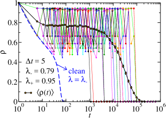
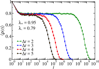
Figure 4: The mean-field density $\rho$ as a function of time for the QCP model. The temporal disorder parameters are $p=\frac{1}{2}$, $\lambda_{-}=0.79$ and $\lambda_{+}=0.95$. In the top panel, $\rho$ is shown for $20$ disorder realizations by the data in various symbols and colors and thin lines for $\Delta t=5$. The average density $\left\langle\rho\right\rangle$ (circles with thick lines) is obtained from $10^{3}$ disorder realizations. In the bottom panel, the density is averaged for $10^{3}$ disorder realizations for different time windows $\Delta t$. In all cases, the lines connecting data symbols are guide to the eyes.

When $\lambda_{-}<\lambda_{c}$ (inactive phase) and $\lambda_{+}\geq\lambda^{*}$ (active phase), the actual system phase is decided by the analysis of the low-density dynamics Eqs. (2) and (9).

For the QCP model, the density decays exponentially in the inactive phase as $\rho\sim e^{-(1-\lambda_{-})t}$ in the $\rho\rightarrow 0$ limit. The active phase appears only when $\lambda=1$ and thus, $\partial_{t}\rho\sim\rho^{2}$. Therefore $\rho$ grows much slower than the exponential. Consequently, the system is in the temporal Griffiths inactive phase.

For the $\sigma$CP model, on the other hand, the fate in the low-density regime is determined by the competition between periods of inactivation, in which $\rho\sim e^{{}^{2\left(\lambda_{-}-\lambda^{*}\right)t}}$, with $\lambda^{*}=\frac{1}{2}$, and periods of activation, in which $\rho\sim e^{{}^{2\left(\lambda_{+}-\lambda^{*}\right)t}}$. Therefore, the system is in the active phase if $\lambda_{+}+\lambda_{-}>2\lambda^{*}$, and it is in the inactive phase if $\overline{\lambda}<\lambda^{*}$. For $\overline{\lambda}=\lambda^{*}$, the system is at the infinite-noise critical point in the same universality class of the temporally disordered CP model Vojta and Hoyos (2015). Evidently, both the inactive and active phases are of temporal Griffiths type. The latter has Griffiths singularities in the same sense as in the contact process model with temporal disorder in which the lifetime of finite systems does not increase exponentially with the system volume (as in the pure active phase) but rather as a power-law Vazquez et al. (2011); Vojta and Hoyos (2015); Barghathi et al. (2016).

Finally let us analyze the case when there is a mix of the metastable ($\lambda_{c}\leq\lambda_{-}<\lambda^{*}$) and active ($\lambda_{+}\geq\lambda^{*}$) phases. Again, we analyze details of the dynamics in the low-density regime. Since the metastable phase behaves just as the inactive one in the low-density regime, the same conclusions are obtained for $\lambda_{-}$ in the inactive and $\lambda_{+}$ in the active phases applies.

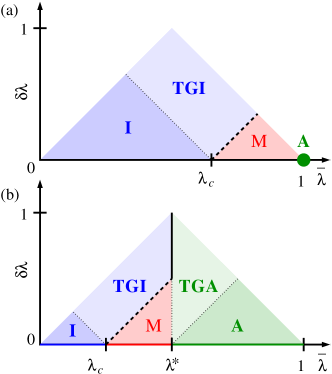
Figure 5: The mean-field phase diagram in the temporally disordered case for the (a) QCP and (b) $\sigma$CP models. The temporal disorder parameters are defined in Eq. (1) with $p=1/2$. In the $\sigma$CP model, we are considering that $a\zeta\left(\sigma\right)>1$, otherwise the metastable phase vanishes. Dashed (solid) lines denote first (second)-order phase transitions. Dotted lines represent crossovers. The parameter space outside the shaded triangle is unphysical. For the QCP model, $\lambda_{c}=\frac{4}{5}$ while it depends on $a$ and $\sigma$ for the $\sigma$CP model; and $\lambda^{*}=\frac{1}{2}$. (A) stands for active, (I) for inactive, (M) for metastable and (TG) for temporal Griffiths.

We are now able to determine the mean-field phase diagram for the QCP and $\sigma$CP models in the presence of temporal disorder as shown in Fig. 5. The dotted line are just crossovers. The inactive and active phases, apart from trivial fluctuations, are akin to the pure phases as discussed in Sec. III.2.1. (Notice however that for the QCP model only the pure active phase exists.) The temporally disordered metastable phase ($\delta\lambda\neq 0$) is also akin to the pure one except for the unpredictability of the fate of the system state when the initial density is between the $\rho_{\infty}^{(U)}\left(\lambda_{+}\right)$ and $\rho_{\infty}^{(U)}\left(\lambda_{-}\right)$ as discussed in Sec. III.2.1. The temporal Griffiths phases have the same nature of their hosting phases but with different behaviors due to rare temporal fluctuations. The dashed lines are metastable—inactive first-order transitions while the solid line in the $\sigma$CP model is a continuous inactive—active phase transition in the infinite-noise universality class of the CP model. Finally, notice that this is the first example of a non-equilibrium phase transition in which there are temporal Griffiths phases in both sides of the transition.

III.3 The probability density distribution for the density of active sites

Due to noise (temporal disorder), the density of active sites greatly fluctuates from sample to sample. It is thus desirable to obtain the probability $R(\rho,t)$ of finding the system density between $\rho$ and $\rho+{\rm d}\rho$ at time $t$.

Let us start by analyzing the cases in which the density can become arbitrarily small in the long-time limit. On then can be obtained $R\left(\rho,t\right)$ using the methods of Ref. Vojta and Hoyos, 2015, where the logistic equations (2) and (9) are linearized. In this approximation, the problem can be mapped into a random walk problem for $x=-\ln\rho$. The nonlinear terms are then replaced by a reflecting wall at the origin ensuring that the walker position is always $x\geq 0$ ($\rho\leq 1$). Therefore, the probability density distribution becomes

$$Q\left(x,t\right)=\sqrt{\frac{2}{\pi\sigma_{v}^{2}n}}e^{-\frac{\left(x-\bar{v}n\right)^{2}}{2\sigma_{a}^{2}n}}-2\frac{\bar{v}}{\sigma_{v}^{2}}e^{\frac{2x\bar{v}}{\sigma_{v}^{2}}}\Phi\left(\frac{-x-vn}{\sigma_{v}\sqrt{n}}\right),$$ (12)

where $\Phi\left(z\right)=\frac{1}{\sqrt{2\pi}}\int_{-\infty}^{z}e^{-\frac{1}{2}y^{2}}{\rm d}y$ is the cumulative normal distribution, $\overline{v}$ and $\sigma_{v}$ are the random walker bias and bare width, respectively, and $n=t/\Delta t$ measures time in units of the time interval $\Delta t$. For the QCP model, $\overline{v}=\overline{\mu\Delta t}=\left(1-\overline{\lambda}\right)\Delta t$ and $\sigma_{v}^{2}=\overline{\left(\mu\Delta t\right)^{2}}-\left(\overline{\mu\Delta t}\right)^{2}=\frac{1}{4}\delta\lambda^{2}\Delta t^{2}$, whereas for the $\sigma$CP model, $\overline{v}=\overline{\left(\mu-\lambda\right)\Delta t}=2\left(\lambda^{*}-\overline{\lambda}\right)\Delta t$ and $\sigma_{v}^{2}=\delta\lambda^{2}\Delta t^{2}$.

The result (12) is accurate far from the reflecting wall and in the long time regime. Hence, in the inactive phase we find that

$$Q_{{\rm inactive}}(x,t)\approx\sqrt{\frac{\Delta t}{2\pi\sigma_{v}^{2}t}}e^{-\frac{(x-\overline{x}_{{\rm inactive}})^{2}}{2\sigma_{v}^{2}t/\Delta t}},$$ (13)

where $\overline{x}_{{\rm inactive}}=\overline{v}n+\frac{\sigma_{v}^{2}}{2\bar{v}}+{\cal O}\left(t^{-1}\right)$ is the walker mean value, with the constant term being the leading correction due to the reflecting wall. Notice that $Q_{{\rm inactive}}$ represents a simple random walker drifting away from the origin as $t\rightarrow\infty$.

The result (12) can also be applied to the active phase close to the transition (which happens only for the $\sigma$CP model for $\overline{\lambda}\apprge\lambda^{*}$), yielding

$$Q_{{\rm active}}(x,t\rightarrow\infty)\approx-\frac{2\bar{v}}{\sigma_{v}^{2}}e^{\frac{2\bar{v}}{\sigma_{v}^{2}}x}=\frac{e^{-x/\overline{x}_{{\rm active}}}}{\overline{x}_{{\rm active}}},$$ (14)

where the walker mean value is $\overline{x}_{{\rm active}}=\frac{\sigma_{v}^{2}}{2\left|\overline{v}\right|}$.

Naturally, Eq. (12) also applies to the transition between the active and inactive phases in which

$$Q_{{\rm critical}}\left(x,t\right)\approx\sqrt{\frac{2\Delta t}{\pi\sigma_{v}^{2}t}}e^{-\frac{x^{2}\Delta t}{2\sigma_{v}^{2}t}}.$$ (15)

Notice that $Q_{{\rm critical}}$ is a half Gaussian distribution which broadens without limit as $t\rightarrow\infty$ illustrating the infinite-noise criticality concept. This also implies that the walker mean value is $\overline{x}_{{\rm critical}}=\sqrt{\frac{2\sigma_{v}^{2}t}{\pi\Delta t}}$.

The result (12) can also be applied to the entire metastable phase of both models if one starts with sufficiently small initial densities [below $\rho_{\infty}^{(U)}(\lambda_{+})$]. In this case, the metastable phase behaves similarly to the inactive phase, and hence, $Q_{{\rm inactive}}$ in Eq. (13) accurately describes the probability density distribution.

We now comment on the cases in which the density $\rho$ does not become small. These happen for the active phase (of the $\sigma$CP model) far away from the inactive phase and for the metastable phase (of both models) provided that one starts with a sufficiently high initial density [above $\rho_{\infty}^{(U)}(\lambda_{-})$]. Clearly, the density of active sites fluctuates between the values $\rho_{\infty}^{(S)}(\lambda_{-})$ and $\rho_{\infty}^{(S)}(\lambda_{+})$. Since the nonlinear terms in Eqs. (2) and (9) are important, it becomes cumbersome to analytically predict the resulting stationary probability density distribution $R(\rho,t)\rightarrow S(\rho)$. For instance, if $\Delta t$ is much greater than the relaxation time required to go from $\rho_{\infty}^{(S)}(\lambda_{-})$ to $\rho_{\infty}^{(S)}(\lambda_{+})$ (and vice-versa), then one mostly finds $\rho$ either very close to $\rho_{\infty}^{(S)}(\lambda_{-})$ or $\rho_{\infty}^{(S)}(\lambda_{+})$. Therefore, $S(\rho)$ is approximately a bimodal distribution peaked around $\rho_{\infty}^{(S)}(\lambda_{-})$ and $\rho_{\infty}^{(S)}(\lambda_{+})$. On the other hand for small $\Delta t$, the system has little time to relax between $\rho_{\infty}^{(S)}(\lambda_{-})$ and $\rho_{\infty}^{(S)}(\lambda_{+})$. Hence, $S(\rho)$ will be peaked at some value between $\rho_{\infty}^{(S)}(\lambda_{-})$ and $\rho_{\infty}^{(S)}(\lambda_{+})$.

Finally, let us analyze the last case in which both $\lambda_{+}$ and $\lambda_{-}$ are in the metastable phase and the initial density is such that $\rho_{\infty}^{(U)}(\lambda_{+})<\rho_{0}<\rho_{\infty}^{(U)}(\lambda_{-})$. As discussed in Sec. III.2, the fate of the activity depends on the details of the temporal disorder. If initially $\lambda=\lambda_{+}$ for a long interval of time, then the density will increase above $\rho_{\infty}^{(U)}(\lambda_{-})$ and thus will remain finite in the stationary regime. Otherwise if $\lambda=\lambda_{-}$ for a long time window, the system then evolves towards the inactive absorbing state. In this case therefore, the distribution of $\rho$ will have two components resulting in $(1-\alpha)S(\rho)+\alpha\rho^{-1}Q_{{\rm inactive}}(e^{-\rho},t)$, where $\alpha$ is the probability that the system evolves into the absorbing state.

We report that we have confirmed all the above results by numerically solving Eqs. (2) and (9) in the presence of temporal disorder via the Euler method and then computing the corresponding probability density distribution. Here, we only show in Fig. 6 the logarithm of the typical density as a function of time for parameters near the transition between the inactive and active phases for the $\sigma$CP model. We also show as solid lines the analytical prediction for the infinite-noise criticality in the long-time regime as discussed after Eqs. (13)—(15). The agreement is remarkable.

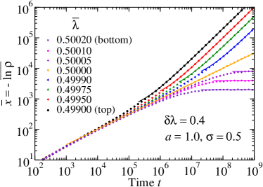
Figure 6: The logarithm of the typical density as a function of the time $t$ for the $\sigma$CP model at the mean-field level. The long-range interaction parameters are $a=1$ and $\sigma=0.5$. The temporal disorder parameters are $\delta\lambda=0.4$ and $\Delta t=10$ [see Eq. (1)]. Data points are averaged over $N=5\times 10^{5}$ disorder realizations. Error bars are about the size of the symbols. Solid lines are the analytical predictions (no fitting parameters) based on the simple random walk picture (see main text).

IV Monte Carlo simulations

Our Monte Carlo simulations were performed in the lowest dimensions in which both models exhibit a first-order phase transition: $d=2$ and $d=1$ for the QCP and the $\sigma$CP models, respectively Windus and Jensen (2007); Fiore and de Oliveira (2007). In all cases, we consider periodic boundary conditions and $\mu=1-\lambda$ with $0<\lambda<1$. For the $\sigma$CP model, we have studied only the case $\sigma=0.5$ and $a=2$.

As discussed in Sec. III, simulations of first-order transitions demands long computational times especially in the presence of temporal disorder. For this reason, our purpose is not to provide precise quantitative numbers, but rather confirm the qualitative scenario of the temporal disorder effects on the first-order phase transitions of Sec. III. Hence, we firstly review the clean system in order to confirm the metastability of the active phase and the algebraically diverging time $T$ in Eq. (8). Then, we provide data supporting the instability of the metastable phase towards the absorbing state when temporal disorder allows for fluctuations into the inactive phase. Finally, we confirmed the infinite-noise criticality governing the transition between the inactive and active phases which takes place in the strong disorder regime of the $\sigma$CP model. We emphasize that it is not our purpose to perform a careful quantitative study. Thus, finite-size effects, unimportant for our discussion, may be strongly present in our data.

IV.1 The Monte Carlo dynamics

The actual dynamics is implemented following Ref. Dickman, 1999. In the 2D square lattice QCP model, an active site, say, $i$, is randomly chosen among all $M$ active sites in the system. With probability $\frac{\mu}{\mu+\lambda}=1-\lambda$, site $i$ becomes inactive whereas, with complementary probability, one of its four nearest neighbor sites, say, $j$, is randomly chosen. If $j$ is active, the system state remains unchanged; if not, it will become active if there is at least one pair of diagonal nearest-neighbors active sites. Otherwise, the state remains unchanged. Finally, the time is increased by $1/M$.

The dynamics in the 1D $\sigma$CP model is very similar. After randomly choosing a site $i$ among all the $M$ active ones, we also choose with equal probability one of the two directions in the lattice. Then, we compute the corresponding activity spreading rate $\lambda_{\ell}=\lambda\left(1+a\ell^{-\sigma}\right)$, with $\ell$ being the distance (in units of lattice spacing) to the next active site in the chosen direction. Afterwards, with probability $\frac{\mu}{\mu+\lambda_{\ell}}=\frac{1-\lambda}{1+\lambda a\ell^{-\sigma}}$ the site $i$ becomes inactive whereas, with complementary probability, the nearest-neighbor site in that chosen direction becomes active (if it was already active, the system state remains unchanged). As in the QCP model, the time is incremented by $1/M$. In these cases, one performs averages over $N_{{\rm MC}}$ different Monte Carlo runs. Since we also aim to study the metastable phase, we need as well to perform simulations starting from a partially filled lattice in which a fraction $0<\rho_{0}<1$ of sites (randomly chosen) is active.

Temporal disorder is implemented as explained in Sec. II. We start with an activity spreading rate drawn from Eq. (1), and whenever the many time increments sum $\Delta t$, a new $\lambda$ is drawn from the same binary distribution.

In the usual clean CP model, one usually performs simulations averaging over $N_{\text{MC}}$ different Monte Carlo runs. In our study, we also need to average over $N_{\text{D}}$ different disorder realizations of the temporal sequence $\{\lambda_{1},\,\lambda_{2},\,\lambda_{3},\,\dots\}$. We verified that our results have no dependence on $N_{\text{MC}}$ as long as $N_{\text{D}}\gg 1$, i.e., it is sufficient using only one Monte Carlo run $N_{{\rm MC}}=1$ for a given temporal sequence $\{\lambda_{i}\}$ provided that the number of different disorder realizations $N_{\text{D}}$ is sufficiently large. In addition, because we want to study the metastable phase, we need as well to perform simulations starting from a partially filled lattice in which a fraction $0<\rho_{0}<1$ of (randomly chosen) sites is active. Therefore, we also need to average over $N_{\text{S}}$ different initial states for each sequence $\{\lambda_{i}\}$. We report that only one different state $N_{\text{S}}=1$ for each temporal sequence is sufficient for obtained unbiased and reliable data as long as the number of different disorder realizations $N_{\text{D}}$ is large. For these reasons, in what follows, we present our data average averaged over $N_{\text{D}}=N$ disorder realizations. This means that only one Monte Carlo run $N_{\text{MC}}=1$ for each of these sequences were performed. For the cases in which $0<\rho_{0}<1$, this also means that $N$ different initial states were considered in the simulation.

IV.2 The clean system

Let us start by analyzing the clean case. The metastability of the active phase near a first-order non-equilibrium phase transition into an absorbing state has been reported in the literature in many different situations Mikhailov (1990); Meerson and Sasorov (2011). It persists in any spatial dimension supporting a first-order phase transition and we have confirmed it in both studied models.

In Fig. 7, we plot the average density of active sites $\rho(t)$ as a function of time $t$ for the QCP model for systems of linear size $L=200$ (we have also used $L=400$ and verified the same conclusions). In the top panel, the initial density is fixed at $\rho_{0}=1$ and the activity spreading rate $\lambda$ is varied. In the remaining panels,$\rho_{0}$ is varied while $\lambda$ is fixed at $0.8613$ (middle) and $0.98$ (bottom). From the top and middle panels we conclude that a first-order phase transition takes place at $0.8610<\lambda_{c}\leq 0.8613$. Interestingly, we conclude from the bottom panel that, in similarity with the mean-field results of Sec. III.1.1, the active phase of the QCP model is entirely metastable (except for the trivial case $\lambda=1$). We have also confirmed it for slightly different implementations of the dynamics and for $\lambda=0.99$. We thus conjecture that this is a general feature of the active phase of the QCP model for any spatial dimension $d\geq 2$.

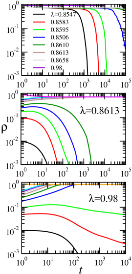
Figure 7: The average density as a function of the simulation time for the QCP. In the top panel, $\rho$ is shown for various $\lambda$ starting for $\rho_{0}=1$. The middle and bottom panels show $\rho$ for $\lambda=0.8613$ and $\lambda=0.98$ and various different initial densities $\rho_{0}$. Data are averaged over $10^{2}$ (for the cases when $\rho$ is large for large $t$)—$10^{5}$ (otherwise) different Monte Carlo runs for systems of linear size $L=200$.

In Fig. 8 we study the $\sigma$CP model for $a=2.0$ and $\sigma=0.5$ for systems size $L=10^{5}$. As in the mean-field approach, we find an active metastable phase in the interval $\lambda_{c}\leq\lambda<\lambda^{*}$ where we have identified $\lambda_{c}\geq 0.643$ and $\lambda^{*}\leq 0.670$.

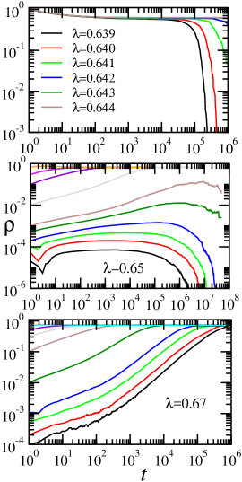
Figure 8: Similar to Fig. 7 but for the $\sigma$CP model with $a=2.0$, $\sigma=0.5$, $L=10^{5}$ and the data are averaged over $10^{3}$—$10^{5}$ different Monte Carlo runs.

We close this section by studying the time $T\sim\left(\lambda_{c}-\lambda\right)^{-\phi}$ required for the system decaying into the absorbing state as $\lambda\rightarrow\lambda_{c}$ (see Fig. 9). We estimate $T$ from the data on the top panels of Figs. 7 and 8 when $\rho(T)=0.1$. (We have used further data with fewer statistics which are not shown.) We find the decay exponent $\phi\approx 1.56(1)$ and $4.52(1)$ for the QCP and $\sigma$CP, respectively. Also, we obtain the transition points $\lambda_{c}=0.8611(3)$ and $0.647(2)$ (for the QCP and $\sigma$CP models, respectively) from the data fitting. Notice that we could not study $T$ for more than 2 orders of magnitude close to the transition point and thus, our estimate may be plagued with large systematic errors.

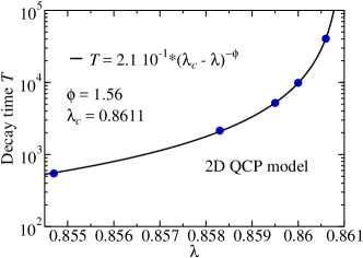
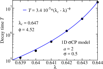
Figure 9: The decay time $T$ to the system toward the absorbing state as a function of s $\lambda$ for the (top) QCP and (bottom) $\sigma$CP models. In both cases, we observe an algebraic behavior of type $(\lambda_{c}-\lambda)^{-\phi}$, where $\phi=1.56(1)$ and $4.52(3)$, respectively.

IV.3 Temporal disorder

We start our study analyzing the 2D QCP model. In panels (a) and (c) of Fig. 10 we confirm the instability of the active phase ($\lambda_{+}=1.0$) with respect to temporal fluctuations into the inactive phase $\lambda_{-}<\lambda_{c}\approx 0.8613$. In panel (a), we show for various $\lambda_{-}$ close to $\lambda_{c}$ that the systems do not decay into the absorbing state up to large times $\sim 10^{7}$, which could be naively interpreted as the system being active. However, as discussed in Eq. (11), this is not the case because the required time for decaying is extremely large. Increasing $\Delta t$ to $10^{4}$ [see panel (c)] reveals the instability of the active phase of the 2D QCP model, just as in the mean-field approach. Panel (b) of Fig. (10) corroborates the metastability of the transition point $\lambda_{-}=\lambda_{c}$ and $\lambda_{+}=1$ between the inactive to the active phase of the QCP model, and therefore, confirms the preservation of the first-order transition character with respect to temporal disorder in the QCP model. Finally, similar to panel (c), in panel (d) we confirm the instability of the metastable phase ($\lambda_{c}<\lambda_{+}=0.95<\lambda^{*}=1$) towards the absorbing state. We report that the transition point $\lambda_{-}=\lambda_{c}$ and $\lambda_{+}=0.95$ is also metastable [as in panel (b)]. Finally,we conclude that the phase diagram for the random 2D QCP model is just as the mean-field one shown in Fig. 5(a) with $\lambda_{c}\approx 0.8613$.

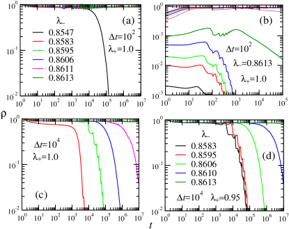
Figure 10: The average density $\rho$ as a function of time $t$ for the 2D QCP model for systems of size $L=200$ averaged over $N_{\text{MC}}=10^{2}$—$10^{5}$ disorder realizations. The disorder parameters [see Eq. (1)] $\lambda_{\pm}$ are indicated in the legends [the one in panel (a) also applies to (c)], $p=\frac{1}{2}$, and $\Delta t=10^{2}$ for panels (a) and (b) and $\Delta t=10^{4}$ for (c) and (d). In all panels the initial density is $\rho_{0}=1$ except in panel (b) where $\rho_{0}$ is varied.

Figure 11 shows the main numerical results for the 1D $\sigma$CP. In panel (a) and (c) we plot $\rho(t)$ for many cases in which $\lambda_{-}<\lambda_{c}\approx 0.643$ is in the inactive phase while $\lambda_{+}=0.650<\lambda^{*}\approx 0.670$ is in the metastable phase. As in the QCP model, the instability of the metastable phase is manifest for the time window studied only when we consider sufficiently large $\Delta t=10^{5}$ as shown in panel (c). Panel (c) is analogous to panel (a) but $\lambda_{+}=0.700>\lambda^{*}$ is in the active phase, and the simulations start from $\rho_{0}=5\times 10^{-5}$. As can be seen, the active phase is stable for $\lambda_{-}\gtrapprox 0.620$. Finally, panel (d) shows $\rho(t)$ starting from different initial conditions for $\lambda_{+}=0.700$ in the active phase and $\lambda_{-}=0.645$ in the metastable one. In this condition, it is clear that the system is effectively active with no indications of bistability. Due to the small range of the metastable phase ($0.643<\lambda<0.670$) we could not reliably study the crossover line between the metastable and active phases analogous to the dotted line in Fig. 5(b).

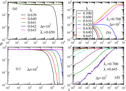
Figure 11: The average density as a function of time for the disordered 1D $\sigma$CP with disorder parameters [see Eq. (1)] $p=\frac{1}{2}$, $\Delta t$ and $\lambda_{\pm}$ are indicated by the legends [with the ones in panel (a) applying for panel (c) as well]. The system size is $L=10^{5}$ averaged over $10^{2}$—$10^{4}$ disorder realizations. In panel (a) and (c), $\lambda_{+}=0.65$ is in the metastable phase while the various $\lambda_{-}\leq\lambda_{c}\approx 0.643$ are in the inactive phase. Panel (b) shows $\rho$ (starting from $\rho_{0}=5\times 10^{-5}$) for various $\lambda_{-}$ in the inactive phase while $\lambda_{+}=0.700$ is in the active one. Panel (d) $\rho$ starting from various different initial conditions for $\lambda_{+}$ in the active phase while $\lambda$ is in the metastable one.

As shown in Fig. 11(b), there is a transition between the active and inactive phases for large $\delta\lambda$. Our final numerical study is to confirm that this transition is in the infinite-noise criticality. We then repeat the study of Fig. 11(b) but starting from the full lattice $\rho_{0}=1$ as shown in Fig. 12. We find that for $\lambda_{-}\approx 0.6195(5)$ the system is critical with average density vanishing (for 2 orders of magnitude in time) as $\rho(t)\sim(\ln t)^{-1}$ ,exactly the same behavior of a system in the infinite-noise criticality of the CP model Vojta and Hoyos (2015); Barghathi et al. (2016).

Figure 12: The average density as a function of time for the $\sigma$CP with $\lambda_{+}=0.7$, $p=\frac{1}{2}$,$\Delta t=10^{2}$ and various distinct values of $\lambda_{-}$. The straight (blue) line has slope $\rho\sim(\ln t)^{-1}$ for more than two orders of magnitude in $t$. The system size is $L=10^{5}$ averaged over $10^{3}$—$3\times 10^{3}$ different disorder realizations.

Finally, we comment on the phase diagram of the random $\sigma$CP. As in Fig. 5(b), the dashed line representing the first-order phase transition is preserved in any dimensions, i.e., its slope independs on $d$. For the studied case ($a=2$ and $\sigma=0.5$ in $d=1$) we find that $\lambda_{c}\approx 0.643$ and $\lambda^{*}\approx 0.670$. We could not determine the dotted line separating the bistability region from the usual active one. For the continuous transition between the inactive and active phase (solid line), we report that we have numerically verified that it tilts to the right favoring the inactive phase. This is expected because inactivation always provide an exponential decay of $\rho$ for any dimension. On the other hand, only in the mean-field approximation the activity spreads exponential fast. For finite dimensions, it can only spread ballistically. Therefore, we expect a smaller active phases when compared with mean field, and thus, the solid line must tilt to the right.

V Conclusions

We have established a general theory of the effect of temporal disorder in discontinuous non-equilibrium phase transitions into an absorbing state. A quantitative analysis is present in the framework of mean-field approach as well as numerical simulations in finite dimensions for two paradigmatic models exhibiting first-order phase transitions, namely the quadratic contact process (QCP) and the contact process with long-range interactions ($\sigma$CP) models. Our work provides an analytical basis for the numerical findings of Ref. de Oliveira and Fiore, 2016 that, in contrast to the spatial disorder, temporal disorder does not forbid discontinuous transition in low dimensional systems. This is not to be mistaken as a weaker effect in comparison since the metastable active phase is replaced by the temporal Griffiths inactive phase.

We have found that temporal disorder noise does not qualitatively affect the phases when the fluctuations are confined within the phases, except for small details in the metastable phase as discussed in Sec. III.2.1.

On the other hand, the metastable phase is always unstable against temporal disorder whenever it allows for fluctuations into the inactive phase. Due to rare temporal fluctuations, the metastable phase becomes a temporal Griffiths inactive phase in which the decay time become exponentially large [see Eq. (11)]. Furthermore, our general mean-field results show that the temporal Griffiths inactive phase is a more general phenomena expected to appear in any non-equilibrium first-order phase transition into an absorbing state.

For the QCP model, the active phase is also unstable against temporal disorder and thus, only exists in the clean limit. As a consequence, the first-order character of the transition is not destabilized by temporal disorder for any disorder strength. In contrast for the $\sigma$CP model, the active phase is robust against small fluctuations into the inactive phase. As a consequence, the first-order transitions is turned into a continuous one when the disorder strength is sufficiently strong. In addition, we have found that the critical behavior belongs to the infinite-noise universality class of the contact process model, but with two Griffiths phases surrounding it.

Finally, we notice that the inactive phase being characterized by an absorbing state is not a necessary condition for our theory. The bistability of the active phase is. Therefore, although we have focused only on two models, we expect that our theory applies to other models exhibiting discontinuous non-equilibrium phases transitions such as, e.g., the ZGB model Ziff et al. (1986) and the majority-vote with inertia model chen and shen (2017).

Appendix A Decaying time near the temporal Griffiths inactive—metastable phase transition

We intend to estimate the average time $\overline{T^{\prime}}$ for decaying when the system undergoes a first-order phase transition from the inactive to the metastable phase in the presence of temporal disorder.

For simplicity, consider the case of binary disorder as defined in Eq. (1) where $\lambda_{-}<\lambda_{c}$ places the system in the inactive phase and $\lambda_{c}<\lambda_{+}<\lambda^{*}$ places the system in the metastable one. In this case, notice there are only three relevant time scales in the problem: the time interval $\Delta t$, the decay time $\tau_{-}$ (related to $\lambda_{-}$) and the relaxation time $\tau_{+}$ (related to $\lambda_{+}$). Precisely, the second is defined as the time required for the system to evolve from $\rho^{(S)}(\lambda_{+})$ to $\rho^{(U)}(\lambda_{+})$ when $\lambda=\lambda_{-}$ while the latter is the other way round when $\lambda=\lambda_{+}$.

Let us consider the case when the disordered system is close to the metastable phase, thus $\lambda_{c}\gg\lambda_{c}-\lambda_{-}>0$ [implying $\tau_{-}\sim T$ in Eq. (8)]. For further simplicity, consider the case $\tau_{+}\ll\Delta t\ll\tau_{-}$ (which could possibly be accomplished when $\lambda_{+}$ is deep in the metastable phase: $\lambda^{*}\gg\lambda^{*}-\lambda_{+}>0$). With those assumptions, the only way of decaying into the absorbing state (starting from the initial condition $\rho_{0}=1$) is via a sufficiently long and continuous sequence of $k=\tau_{-}/\Delta t$ inactive time intervals ($\lambda=\lambda_{-}$) such that $\rho$ becomes less than $\rho^{(U)}(\lambda_{+})$ afterwards.

Since this long sequence is rare, the waiting time $T^{\prime}$ can be extremely long as we show in the following. Consider intervals of duration $\tau_{-}$ which appear with probability $p_{\tau}=p^{k}$, with $p$ being the probability for an interval being of inactive type [see Eq. (1)]. Then, starting from an active state, the probability that the system decays just after the $n$th of such time intervals is

$$P_{n}=\left(1-p_{\tau}\right)^{n-1}p_{\tau}.$$ (16)

Thus, the average waiting time for decaying into the absorbing state is

$$\overline{T^{\prime}}\approx\tau_{-}\sum_{n=1}^{\infty}nP_{n}=\tau_{-}p^{-\frac{\tau_{-}}{\Delta t}},$$

and we recall that $\tau_{-}\sim T$.

References

- Kussell and Vucelja (2014) E. Kussell and M. Vucelja, Reports on Progress in Physics 77, 102602 (2014).
- Pastor-Satorras et al. (2015) R. Pastor-Satorras, C. Castellano, P. Van Mieghem, and A. Vespignani, Rev. Mod. Phys. 87, 925 (2015).
- Sen and Chakrabarti (2013) P. Sen and B. K. Chakrabarti, Sociophysics: An Introduction (Oxford University Press, Oxford, UK, 2013).
- Ziff et al. (1986) R. M. Ziff, E. Gulari, and Y. Barshad, Phys. Rev. Lett. 56, 2553 (1986).
- Tang and Leschhorn (1992) L.-H. Tang and H. Leschhorn, Phys. Rev. A 45, R8309 (1992).
- Buldyrev et al. (1992) S. V. Buldyrev, A.-L. Barabási, F. Caserta, S. Havlin, H. E. Stanley, and T. Vicsek, Phys. Rev. A 45, R8313 (1992).
- Pomeau (1986) Y. Pomeau, Physica D 23, 3 (1986).
- Marro and Dickman (1999) J. Marro and R. Dickman, Nonequilibrium Phase Transitions in Lattice Models (Cambridge University Press, Cambridge, England, 1999).
- Henkel et al. (2008) M. Henkel, H. Hinrichsen, and S. Lübeck, Non-Equilibrium Phase Transitions, Volume I: Absorbing Phase Transitions (Springer, Dordrecht, The Netherlands, 2008).
- Ódor (2004) G. Ódor, Rev. Mod. Phys. 76, 663 (2004).
- Kinzel (1985) W. Kinzel, Zeitschrift für Physik B Condensed Matter 58, 229 (1985).
- Noest (1986) A. J. Noest, Phys. Rev. Lett. 57, 90 (1986).
- Hinrichsen (2000) H. Hinrichsen, Braz. J. Phys. 30, 69 (2000).
- Takeuchi et al. (2007) K. A. Takeuchi, M. Kuroda, H. Chaté, and M. Sano, Phys. Rev. Lett. 99, 234503 (2007).
- Hooyberghs et al. (2003) J. Hooyberghs, F. Iglói, and C. Vanderzande, Phys. Rev. Lett. 90, 100601 (2003).
- Vojta and Dickison (2005) T. Vojta and M. Dickison, Phys. Rev. E 72, 036126 (2005).
- Vojta and Lee (2006) T. Vojta and M. Y. Lee, Phys. Rev. Lett. 96, 035701 (2006).
- Hoyos (2008) J. A. Hoyos, Phys. Rev. E 78, 032101 (2008).
- de Oliveira and Ferreira (2008) M. M. de Oliveira and S. C. Ferreira, Journal of Statistical Mechanics: Theory and Experiment 2008, P11001 (2008).
- Vojta et al. (2009) T. Vojta, A. Farquhar, and J. Mast, Phys. Rev. E 79, 011111 (2009).
- Vazquez et al. (2011) F. Vazquez, J. A. Bonachela, C. López, and M. A. Muñoz, Phys. Rev. Lett. 106, 235702 (2011).
- Vojta and Hoyos (2015) T. Vojta and J. A. Hoyos, EPL (Europhysics Letters) 112, 30002 (2015).
- Barghathi et al. (2016) H. Barghathi, T. Vojta, and J. A. Hoyos, Phys. Rev. E 94, 022111 (2016).
- Solano et al. (2016) C. M. D. Solano, M. M. de Oliveira, and C. E. Fiore, Phys. Rev. E 94, 042123 (2016).
- Hoenicke and Figueiredo (2000) G. L. Hoenicke and W. Figueiredo, Phys. Rev. E 62, 6216 (2000).
- Villa Martín et al. (2014) P. Villa Martín, J. A. Bonachela, and M. A. Muñoz, Phys. Rev. E 89, 012145 (2014).
- de Oliveira and Fiore (2016) M. M. de Oliveira and C. E. Fiore, Phys. Rev. E 94, 052138 (2016).
- Harris (1974) T. E. Harris, Ann. Prob. 2, 969 (1974).
- Schlögl (1972) F. Schlögl, Zeitschrift für Physik 253, 147 (1972).
- Ginelli et al. (2005) F. Ginelli, H. Hinrichsen, R. Livi, D. Mukamel, and A. Politi, Phys. Rev. E 71, 026121 (2005).
- Windus and Jensen (2007) A. Windus and H. J. Jensen, Journal of Physics A: Mathematical and Theoretical 40, 2287 (2007).
- Fiore and de Oliveira (2007) C. E. Fiore and M. J. de Oliveira, Phys. Rev. E 76, 041103 (2007).
- Dickman (1999) R. Dickman, Phys. Rev. E 60, R2441 (1999).
- Mikhailov (1990) A. S. Mikhailov, in Foundations of Synergetics I: Distributed Active Systems, Vol. 51, edited by Hermann Haken (Springer-Verlag, Berlin Heidelberg, 1990).
- Meerson and Sasorov (2011) B. Meerson and P. V. Sasorov, Phys. Rev. E 83, 011129 (2011).
- chen and shen (2017) H. Chen, C. Shen, H. Zhang, G. Li, Z. Hou and J. Kurths, Phys. Rev. E 95, 042304 (2017).