Parameter-uniform numerical methods for singularly perturbed parabolic problems with incompatible boundary-initial data

Abstract

Numerical approximations to the solution of a linear singularly perturbed parabolic reaction-diffusion problem with incompatible boundary-initial data are generated, The method involves combining the computational solution of a classical finite difference operator on a tensor product of two piecewise-uniform Shishkin meshes with an analytical function that captures the local nature of the incompatibility. A proof is given to show almost first order parameter-uniform convergence of these numerical/analytical approximations. Numerical results are given to illustrate the theoretical error bounds.

1 Introduction

We examine singularly perturbed parabolic problems in one space dimension, with an incompatibility between the initial condition and a boundary condition. These problems arise in mathematical models in fluid dynamics [8] and, in particular, models for flow in porous media [3]. The solutions of these problems typically exhibit boundary layers, initial layers and initial-boundary layers. In this paper we are interested in constructing a parameter-uniform numerical algorithm [2] for this class of singularly perturbed problems.

Numerical methods generate finite dimensional approximations $U^{N}$ (where $N$ is the number of mesh elements used in each coordinate direction) to the continuous solution $u$ at the selected nodal points within the continuous domain $\bar{Q}$. A global approximation $\bar{U}^{N}$ can also be created, using a user chosen choice of interpolating basis functions. In this paper, we shall simply employ bilinear basis functions. Parameter-uniform numerical methods [2] satisfy a theoretical error bound of the form:

$$\|u-\bar{U}^{N}\|_{\bar{Q}}\leq CN^{-p},\quad p>0;$$

where $\|\cdot\|_{\bar{Q}}$ is the $L_{\infty}$ norm on the closed domain $\bar{Q}$, $C$ is a generic constant, which depends on the problem data but is independent of $N$ and the singular perturbation $\varepsilon$. We emphasize that this error bound estimates the pointwise error at all points in the domain $\bar{Q}$ of the continuous solution. Parameter-uniform convergence at the nodes is a necessary, but not a sufficient, condition for parameter-uniform global convergence. If a numerical method is parameter-uniform at the nodes, then the distribution of the mesh points and the selected form of interpolation will determine whether the method is globally parameter-uniform or not.

Within the literature on singularly perturbed problems, there are two common approaches to designing a parameter-uniform method: fitted operator (see e.g. [15]) or fitted mesh methods [2]. Fitted operator methods tend to use a quasi-uniform discretization of the domain and incorporate analytical information about the solution character within the layers, into the choice of special basis functions (in a finite element framework) or (in the case of finite differences) by choosing a special finite difference operator that is exact in the case of constant coefficient one dimensional model problems. On the other hand, fitted mesh methods use a priori information about the layer structure to construct an appropriate non-uniform distribution of the mesh points.

For some classes of singularly perturbed problems with boundary layers, fitted operator methods on a uniform mesh exist which satisfy a parameter-uniform error bound at the nodes, but these fitted operator methods are not globally parameter-uniformly convergent [2], when some form of polynomial interpolation is employed. In the case of one-dimensional problems not containing characteristic boundary layers, global convergence can be guaranteed if one subsequently incorporates exponential splines to form the interpolant [17]; but this form of non-polynomial spline interpolation is difficult to extend to elliptic problems in higher dimensions. Moreover, a nodally parameter-uniform fitted operator method cannot be constructed for a class of singularly perturbed heat equations, if one only uses a uniform mesh [2, 13]. This same impasse is faced when dealing with elliptic problems, whose solutions contain characteristic boundary layers. However, a fitted piecewise-uniform Shishkin mesh coupled with a classical discrete operator produces a parameter-uniform numerical method for singularly perturbed heat equations [14] and for elliptic problems with characteristic layers [16]. Moreover, parameter-uniform numerical methods, using an appropriate Shishkin mesh have been designed for a wide class of singularly perturbed problems [11]. These problem classes include problems with both boundary and initial layers.

To establish pointwise parameter uniform error bounds on numerical approximations to the solutions of singularly perturbed parabolic problems, most publications assume second level compatibility conditions and sufficient regularity of the data so that the solution is in $C^{4+\gamma}(\bar{Q})$ in the closed domain $\bar{Q}$. Interested readers are referred, for example, to [19]. In the case of singularly perturbed parabolic problems in one space dimension and using appropriate fitted meshes, these compatibility constraints can be relaxed to zero order, without an adverse effect on the rate of uniform convergence [18]. Hence, parameter-uniform numerical methods exist when the boundary and initial data are simply assumed to be continuous.

However, there are difficulties with constructing a fitted mesh method for problems with an incompatibility between the initial and a boundary condition; or for a problem with a discontinuity in a boundary or the initial condition [9, 10]. Hemker and Shishkin [10] constructed a fitted operator method on a uniform mesh, which is nodally parameter-uniform for a singularly perturbed heat equation with a discontinuity in the initial condition; but the method is not globally parameter-uniform, using bilinear interpolation. An extension of this fitted operator method to a fitted operator method on a fitted piecewise-uniform mesh was constructed in [5], but this again failed to be parameter-uniform globally, using bilinear interpolation. The interpolation failed to produce an accurate global approximation in a neighbourhood of the point, where the initial condition and a boundary condition were incompatible.

Another approach to dealing with a problem having discontinuous data is to replace the problem with a regularized problem with continuous data [6]. This approach is strongly related to the penalty method discussed in [1]. For example, the problem

$$u_{t}-\varepsilon u_{xx}=f(x,t),\qquad x,t>0;$$

$$u(0,t)=0,\ t>0;\quad u(x,0)=1,\ x>0$$

can be approximated by the solution $u^{r}$ of the regularized problem:

$$u^{r}_{t}-\varepsilon u^{r}_{xx}=f(x,t),\qquad x,t>0;$$

$$u^{r}(0,t)=0,\ t>0;\quad u^{r}(x,0)=1-e^{-x/\sqrt{\varepsilon}},\ x\geq 0.$$

Parameter-uniform numerical approximations to $u^{r}$ can be generated, but (see [6]) these approximations are only accurate approximations to $u$ outside a neighbourhood of the point $(0,0)$. In other words, this approach will not generate parameter-uniform global approximations to the original problem with an incompatibility between the boundary and initial data.

In this paper, we examine an alternative approach to dealing with this problem class, which uses an idea examined numerically in [4] in the non-singularly perturbed case (set $\varepsilon=1$). Given a differential operator $L$, the solution $u$ of the continuous problem

$$Lu=f,\ \hbox{in}\ Q,\quad u=g,\ \hbox{on}\ \bar{Q}\setminus Q=:\partial Q,\quad\hbox{where}\quad g\notin C^{0}(\partial Q);$$

is written as the sum of two components $u=s+y$. The function $s$ matches the incompatibility in the solution $u$ and the other term $y$ satisfies the singularly perturbed problem

$$Ly=f-Ls,\ \hbox{in}\ Q,\quad y=g-s,\ \hbox{on}\ \bar{Q}\setminus Q,\quad\hbox{where}\quad g-s\in C^{0}(\partial Q).$$

In this paper, we design a parameter-uniform numerical method for this secondary problem, which generates a global approximation $\bar{Y}$ to $y$. In this way, we can generate parameter-uniform numerical approximations $s+\bar{Y}$ to the solution $u$ of a singularly perturbed problem with an incompatibility between the initial condition and a boundary condition. Note that here we restrict the discussion to problems in one space dimension. Extensions of the method to two space dimensions are not obvious [1] and require further investigation.

The rest of the paper is structured as follows. In the next section, we define the problem class to be examined, we decompose the continuous solution into various components and we derive parameter-explicit bounds on the derivatives of each of these components. In Section 3, we construct the numerical method and we establish a parameter-uniform bound on the error. In Section 4, we present the results of some numerical experiments with a representative test problem. For the sake of completeness, we write out the compatibility conditions of levels zero, one and two in the first appendix. Finally, in a second appendix, we present some properties of an analytical function which are used in the proof of Theorem 3.

Notation. Throughout the paper, $C$ denotes a generic constant that is independent of the singular perturbation parameter $\varepsilon$ and of all discretization parameters. The $L_{\infty}$ norm on the domain $D$ shall be denoted by $\|\cdot\|_{D}$ and the subscript is omitted if the domain is $\bar{Q}$.

2 Continuous problem

Consider the singularly perturbed parabolic problem: Find $u:\bar{Q}\rightarrow\mathbb{R}$ with $Q:=(0,1)\times(0,T],$ such that

$$Lu:=\varepsilon(u_{t}-u_{xx})+b(x,t)u=f(x,t),\quad(x,t)\in Q;$$ (1a)

$$u(0,t)=g_{L}(t),\ u(1,t)=g_{R}(t)\ t\geq 0,\quad u(x,0)=\phi(x),\ 0<x<1;$$ (1b)

$$\phi(0^{+})\neq g_{L}(0),\quad\phi(1^{-})=g_{R}(0),$$ (1c)

$$b_{x}(0,0)=0\quad\hbox{and}\quad b(x,t)>\beta>0,\ \forall t\geq 0;$$ (1d)

$$f,b\in C^{4+\gamma}(\bar{Q}),\ g_{L},g_{R}\in C^{2}[0,T],\ \phi\in C^{4}[0,1].$$ (1e)

Observe that the solution of this problem is discontinuous at the corner $(0,0)$ of the domain $\bar{Q}$. We define the related constant coefficient differential operator

$$L_{0}z:=\varepsilon(z_{t}-z_{xx})+b(0,0)z,$$ (2)

so that (by (1d))

$$|(L-L_{0})z(x,t)|\leq C(x^{2}+t)|z(x,t)|.$$

It is important to point out that the coefficient $b(x,t)$ can depend on both the space and time variables. In the special case where this coefficient only depends on time, then the singularity associated with the incompatibility at $(0,0)$ can be found analytically.

We also assume the compatibility conditions at the point $(1,0)$

$$\varepsilon(g_{R}^{\prime}(0^{+})-\phi_{xx}(1^{-}))+b(1,0)g_{R}(0)=f(1,0);$$ (3)

$$\varepsilon(g_{R}^{\prime\prime}(0^{+})-\phi_{xxxx}(1^{-}))+b(1,0)(g^{\prime}_{R}(0)+\phi_{xx}(1^{-}))$$

$$\hskip 5.69046pt+b_{t}(1,0)g_{R}(0)+2b_{x}(1,0)\phi_{x}(1^{-})+b_{xx}(1,0)\phi(1^{-})=\bigl{(}f_{t}+f_{xx}\bigr{)}(1,0);$$ (4)

Here we simply assume these additional compatibility conditions in order to concentrate on the issues near $(0,0)$, associated with the lack of corresponding compatibility conditions being assumed at $(0,0)$. The numerical method presented below will satisfy the same error bound, established in Theorem 4, even when the data does not satisfy the constraints (3), (4). In this section, the solution $u$ is decomposed in a sum of terms, some associated with the layers in the solution and some terms (denoted below by $A_{0}z_{0}(x,t)+A_{1}z_{1}(x,t)+A_{2}z_{2}(x,t)$) associated with the lack of compatibility being assumed at $(0,0)$. If we did not assume (3), (4), then additional terms of the form $A^{R}_{1}z_{1}(1-x,t)+A^{R}_{2}z_{2}(1-x,t)$ would be included in the expansion of the continuous solution; and the influence of these additional terms on the numerical analysis, could be tracked in the exact same way as the terms $A_{1}z_{1}(x,t)+A_{2}z_{2}(x,t)$ are handled in the error analysis below. Hence, it is solely for the sake of clarity of exposition in this section of the paper, that we assume the compatibility conditions (3), (4).

Decompose the solution of (1) into the sum

$$u=A_{0}e^{-\frac{b(0,0)t}{\varepsilon}}\operatorname{erfc}\left(\frac{x}{2\sqrt{t}}\right)+y,\quad A_{0}:=g_{L}(0)-\phi(0^{+}),$$ (5)

where $\operatorname{erfc}(z)$ is the complimentary error function

$$\operatorname{erfc}(z):=\frac{2}{\sqrt{\pi}}\int_{s=z}^{\infty}e^{-s^{2}}\ ds.$$

Note that the function

$$z_{0}(x,t):=e^{-\frac{b(0,0)t}{\varepsilon}}\operatorname{erfc}\left(\frac{x}{2\sqrt{t}}\right)$$

is the first of a family of functions defined as the solutions of the constant coefficient homogeneous quarter plane problems, where for all $n=0,1,2,\ldots$

$$L_{0}z_{n}=0,\ x,t>0,\ z_{n}(0,t)=t^{n}e^{-\frac{b(0,0)t}{\varepsilon}},\ t>0,\ z_{n}(x,0)=0,\ x>0.$$ (6)

In Appendix 2, we explicitly write out several derivatives of these functions and we discuss the regularity of these functions.

In this section, we establish a priori bounds on the derivatives of the continuous function $y:=u-A_{0}z_{0}$, which satisfies the problem

$$Ly=f(x,t)-A_{0}(L-L_{0})z_{0}(x,t),\ \hbox{ in }Q;$$ (7a)

$$y(0,t)=g_{L}(t)-A_{0}e^{-\frac{b(0,0)t}{\varepsilon}},\quad y(1,t)=g_{R}(t)-A_{0}z_{0}(1,t),\quad t\geq 0;$$ (7b)

$$y(x,0)=\phi(x),\quad 0<x<1.$$ (7c)

We introduce extended domains, where various subcomponents of the solution $y$ will be defined: For arbitrary positive constants $p,q,r$,

$$\bar{Q}^{*}:=[-p,1+q]\times[-r,T];\ \bar{Q}^{*}_{S}:=[0,1]\times[-r,T];\ \bar{Q}^{*}_{B}:=[-p,1+q]\times[0,T].$$

To avoid excessive notation, we shall denote smooth extensions of the functions $b,f$ to some larger domain by $b^{*},f^{*}$ (such that $f^{*}|_{\bar{Q}}\equiv f$), even those these extensions will be taken over different domains.

The solution of (7) can be decomposed into a sum of a regular component $v$ and several layer components $w$ (with a subscript to identify the location of the layer) defined as follows:

$$y=v+w_{L}+w_{R}+w_{I}+w_{IB};$$ (8a)

where the regular component $$v$$ satisfies the problem

$$L^{*}v^{*}=f^{*},\quad\hbox{ in }Q^{*},\quad v^{*}=v^{*},\ \hbox{ on }\partial Q^{*}.$$ (8b)

The boundary/initial values for the regular component are determined from the reduced solution $$v_{0} v_{1} v^{*}=v^{*}_{0}+\varepsilon v^{*}_{1} v_{0} v_{1}$$ and a correction . We write , where the reduced solution and the correction are defined via

$$v^{*}_{0}=\bigl{(}\frac{f}{b}\bigr{)}^{*},\hbox{ in }Q^{*};$$ (8c)

$$L^{*}v^{*}_{1}=(v_{0})^{*}_{xx}-(v_{0})^{*}_{t},\quad\hbox{ in }Q^{*},\quad v^{*}_{1}=0,\ \hbox{ on }\partial Q^{*}.$$ (8d)

The boundary layer components $$w_{L},w_{R}$$ satisfy the homogeneous problems

$$L^{*}w^{*}_{R}=L^{*}w^{*}_{L}=0,\ \hbox{ in }Q^{*}_{S};$$ (8e)

$$w^{*}_{L}(0,t)=(y-v^{*})^{*}(0,t),\ w^{*}_{L}(x,-r)=0,\ w^{*}_{L}(1,t)=0,\ \hbox{ on }\partial Q_{S}^{*};\quad$$ (8f)

$$w^{*}_{R}(0,t)=0,\ w^{*}_{R}(x,-r)=0,\ w^{*}_{R}(1,t)=(y-v^{*})^{*}(1,t),\ \hbox{ on }\partial Q_{S}^{*}.\quad$$ (8g)

The initial layer function $$w_{I}$$ satisfies the problem

$$L^{*}w^{*}_{I}=0\,\quad\hbox{in}\quad Q^{*}_{B};$$ (8h)

$$w^{*}_{I}(-p,t)=0,\ w^{*}_{I}(x,0)=(y-v^{*})^{*}(x,0),\ w^{*}_{I}(1+q,t)=0,\hbox{ on }\partial Q_{B}^{*}.$$ (8i)

Having defined the problems over the extended domains, to avoid compatibility issues, all of these components are in $$C^{4+\gamma}(\bar{Q})$$.

Finally, the initial-boundary layer component $w_{IB}$ satisfies the problem

$$Lw_{IB}=-A_{0}(L-L_{0})z_{0}(x,t),\quad(x,t)\in Q;$$ (8j)

$$w_{IB}(0,t)=-w^{*}_{I}(0,t),\quad w_{IB}(1,t)=-w^{*}_{I}(1,t),\quad t\geq 0;$$ (8k)

$$w_{IB}(x,0)=-w^{*}_{L}(x,0)-w^{*}_{R}(x,0),\quad 0<x<1.$$ (8l)

The regularity of this key component $w_{IB}$ is discussed below in Theorem 3.

Theorem 1.

For all $0\leq i+2j\leq 4$, we have the following bounds.

For the regular component $$v\in C^{4+\gamma}(\bar{Q})$$,

$$\left\|\frac{\partial^{i+j}v}{\partial x^{i}\partial t^{j}}\right\|\leq C\left(1+\varepsilon^{1-(i/2+j)}\right);$$ (9a)

and, for all points $$(x,t)\in Q w_{L},w_{R}\in C^{4+\gamma}(\bar{Q})$$, the boundary layer components satisfy

$$|w_{L}(x,t)|\leq Ce^{-\sqrt{\frac{\beta}{\varepsilon}}x};\quad|w_{R}(x,t)|\leq Ce^{-\sqrt{\frac{\beta}{\varepsilon}}(1-x)};\,$$ (9b)

$$\left|\frac{\partial^{i+j}}{\partial x^{i}\partial t^{j}}w_{L}(x,t)\right|\leq C\varepsilon^{-(i/2+j)}e^{-\sqrt{\frac{\beta}{\varepsilon}}x},$$ (9c)

$$\left|\frac{\partial^{i+j}}{\partial x^{i}\partial t^{j}}w_{R}(x,t)\right|\leq C\varepsilon^{-(i/2+j)}e^{-\sqrt{\frac{\beta}{\varepsilon}}(1-x)}.$$ (9d)

In addition, for $$1\leq j\leq 2$$, the time derivatives satisfy

$$\max\left\{\left\|\frac{\partial^{j}w_{L}}{\partial t^{j}}\right\|,\left\|\frac{\partial^{j}w_{R}}{\partial t^{j}}\right\|\right\}\leq C\varepsilon^{1-j}.$$ (9e)

Proof.

Using the stretched variables

$$\zeta=\frac{x}{\sqrt{\varepsilon}}\quad\hbox{and}\quad\eta=\frac{t}{\varepsilon}$$

problem (8d) transforms into the problem

$$\tilde{v}_{\zeta\zeta}-\tilde{v}_{\tau}+\tilde{b}\tilde{v}=\tilde{f}_{1},\quad\hbox{in}\left(\frac{-p}{\sqrt{\varepsilon}},\frac{1+q}{\sqrt{\varepsilon}}\right)\times\left(\frac{-r}{\varepsilon},\frac{T}{\varepsilon}\right],$$

where

$$\tilde{v}(\zeta,\tau)=v^{*}_{1}(x,t)\quad\hbox{and}\quad\tilde{f}_{1}(\zeta,\tau)=(v_{0})^{*}_{xx}-(v_{0})^{*}_{t}.$$

Applying the a priori bounds [12] on the derivatives of the solution $\tilde{v}$, and transforming back to the original variables $(x,t)$, we get that

$$\left\|\frac{\partial^{i+j}v_{1}^{*}}{\partial x^{i}\partial t^{j}}\right\|\leq C\left(1+\varepsilon^{-(i/2+j)}\right),\ 0\leq i+2j\leq 4,$$ (10)

and we have deduced the bounds (9a) on the derivatives of the regular component. A maximum principle, the assumption $b(x,t)>\beta$, the corresponding bounds (10) and the argument from [14, Theorem 4] yield the bounds on the boundary layer components $w_{L},w_{R}$ (9b)-(9d).

Note that

$$L^{*}\frac{\partial w^{*}_{L}}{\partial t}=-\frac{\partial b}{\partial t}w^{*}_{L},\ \hbox{ in }Q^{*}_{S};$$

$$\frac{\partial w^{*}_{L}}{\partial t}(0,t)=\frac{\partial(y-v^{*})^{*}}{\partial t}(0,t),\ \frac{\partial w^{*}_{L}}{\partial t}(x,-r)=0,\ \frac{\partial w^{*}_{L}}{\partial t}(1,t)=0,\ \hbox{ on }\partial Q_{S}^{*}.$$

Using the stretched variables and the earlier argument, we deduce that

$$\left\|\frac{\partial^{i+j}}{\partial x^{i}\partial t^{j}}\Bigl{(}\frac{\partial w^{*}_{L}}{\partial t}\Bigr{)}\right\|\leq C\left(1+\varepsilon^{-(i/2+j)}\right),\ 0\leq i+2j\leq 2,$$

which yields the final bounds (9e) on the time derivatives of the layer components. ∎

Theorem 2.

For the initial layer component $$w_{I}\in C^{4+\gamma}(\bar{Q})$$ and

$$|w_{I}(x,t)| \leq Ce^{-\frac{\beta t}{\varepsilon}},\,\ (x,t)\in Q;$$ (11a)

$$\left|\frac{\partial^{i+j}w_{I}}{\partial x^{i}\partial t^{j}}(x,t)\right| \leq C\varepsilon^{-i/2}\varepsilon^{-j}e^{-\frac{\beta t}{\varepsilon}},\ 0\leq i+2j\leq 4;$$ (11b)

$$\left|\frac{\partial^{i}w_{I}}{\partial x^{i}}(x,t)\right| \leq C(1+\varepsilon^{1-i/2})e^{-\frac{\beta t}{\varepsilon}},\quad i=1,2,3,4.$$ (11c)

Proof.

Note that for the initial condition $\|w^{*}_{I}(x,0)\|\leq C$, the boundary conditions $w^{*}_{I}(-p,t)=w^{*}_{I}(1+q,t)=0$ and

$$L^{*}e^{-\frac{\beta t}{\varepsilon}}=(b^{*}(x,t)-\beta)e^{-\frac{\beta t}{\varepsilon}}\geq 0.$$

The bound (11a) follows from the maximum principle.

To deduce bounds on the derivatives of $w_{I}$, we repeat the argument from [14]. Transforming to the stretched variables $\zeta=x/\sqrt{\varepsilon},\eta=t/\varepsilon$ we have

$$\left(\frac{\partial}{\partial\eta}-\frac{\partial^{2}}{\partial\zeta^{2}}+\tilde{b}I\right)(\tilde{w}^{*}_{I})=0,\quad\hbox{in }\left(-\frac{p}{\sqrt{\varepsilon}},\frac{1+q}{\sqrt{\varepsilon}}\right)\times\left(0,\frac{T}{\varepsilon}\right],$$

$$\left|\frac{\partial^{i}\tilde{w}^{*}_{I}}{\partial\zeta^{i}}(\zeta,0)\right|\leq C,\qquad 0\leq i\leq 4.$$

From the interior Schauder estimates [12, §4.10], we have that for any neighbourhood $\tilde{N}_{\delta}\in\left(-\frac{p}{\sqrt{\varepsilon}},\frac{1+q}{\sqrt{\varepsilon}}\right)\times\left(1,T/\varepsilon\right)$

$$\left\|\frac{\partial^{i+j}\tilde{w}^{*}_{I}}{\partial\eta^{j}\partial\zeta^{i}}\right\|_{\tilde{N}_{\delta}}\leq C\Bigl{\|}\tilde{w}^{*}_{I}\Bigr{\|}_{\tilde{N}_{2\delta}}\leq Ce^{-\beta(\eta-2\delta)}\leq Ce^{-\beta\eta};\quad 1\leq i+2j\leq 4;$$

and in the initial layer region $(-\frac{p}{\sqrt{\varepsilon}},\frac{1+q}{\sqrt{\varepsilon}})\times(0,1]$, simply use

$$\Bigl{\|}\frac{\partial^{i+j}\tilde{w}^{*}_{I}}{\partial\eta^{j}\partial\zeta^{i}}\Bigr{\|}_{\tilde{N}_{\delta}}\leq C\leq Ce^{-\beta\eta},\qquad\hbox{as}\quad\eta\leq 1.$$

After transforming back to the original variables, we have thus established the pointwise bounds (11b) on the partial derivatives of $w_{I}$.

To establish sharper bounds on the space derivatives of $w_{I}$, we differentiate the differential equation (8h) with respect to the space variable and formulate parabolic problems for $(w^{*}_{I})_{x}$ and $(w^{*}_{I})_{xx}$.

$$L^{*}\bigl{[}(w^{*}_{I})_{x}\bigr{]}=-b^{*}_{x}w^{*}_{I},\hbox{ in }Q^{*}_{B};\|(w^{*}_{I})_{x}(x,0)\|\leq C,\ -p<x<1+q.$$

The extensions can be constructed so that $\|(w^{*}_{I})_{x}(-p,t)\|\leq C,\|(w^{*}_{I})_{x}(1+q,t)\|\leq C$. Repeating the above argument with the maximum principle and the stretched variables, one can deduce that

$$\left|\frac{\partial^{i+j}}{\partial x^{i}\partial t^{j}}\left(\frac{\partial w^{*}_{I}}{\partial x}\right)(x,t)\right|\leq C\left(1+\varepsilon^{-(i/2+j)}\right)e^{-\frac{\beta t}{\varepsilon}},\ 0\leq i+2j\leq 2.$$

Note further,

$$L^{*}\bigl{[}(w^{*}_{I})_{xx}\bigr{]}=-b^{*}_{xx}w^{*}_{I}-2b^{*}_{x}(w^{*}_{I})_{x},\hbox{ in }Q^{*}_{B}$$

$$(w^{*}_{I})_{xx}(-p,t)=0,\quad(w^{*}_{I})_{xx}(1+q,t)=0,\ t\geq 0$$

$$(w^{*}_{I})_{xx}(x,0)=((y-v^{*})^{*}(x,0))_{xx},\ -p<x<1+q.$$

Repeating the argument, one can deduce that

$$\left|\frac{\partial^{i+j}}{\partial x^{i}\partial t^{j}}\left(\frac{\partial^{2}w^{*}_{I}}{\partial x^{2}}\right)(x,t)\right|\leq C\left(1+\varepsilon^{-(i/2+j)}\right)e^{-\frac{\beta t}{\varepsilon}},\ 0\leq i+2j\leq 2,$$

which complete the proof. ∎

We consider now the initial-boundary layer component $w_{IB}$ defined in (8j)-(8l). As $y$ is continuous and the components $v,w_{L},w_{R},w_{I}$ are smooth, zero-order compatibility conditions (for $w_{IB}$) are satisfied. We further decompose the initial-boundary layer term via

$$w_{IB}(x,t)=A_{1}z_{1}(x,t)+w_{C}(x,t),$$

where the constant $A_{1}$ is specified in (35) and the function $z_{1}$ is defined in (6). Note that $z_{1}\not\in C^{2+\gamma}(\bar{Q})$.

Theorem 3.

The initial-boundary layer component $w_{C}\in C^{2+\gamma}(\bar{Q})$. For all $(x,t)\in\bar{Q}$

$$|w_{C}(x,t)|\leq Ce^{-\frac{\beta t}{\varepsilon}};$$ (12a)

and

$$\left|\frac{\partial^{2}w_{C}}{\partial x^{2}}(x,t)\right|+\left|\frac{\partial w_{C}}{\partial t}(x,t)\right|\leq C+C\varepsilon^{-1}\left(e^{-\sqrt{\frac{\beta}{\varepsilon}}x}+e^{-\sqrt{\frac{\beta}{\varepsilon}}(1-x)}+e^{-\frac{\beta t}{\varepsilon}}\right)$$ (12b)

$$\left|\frac{\partial^{4}w_{C}}{\partial x^{4}}(x,t)\right|+\left|\frac{\partial^{2}w_{C}}{\partial t^{2}}(x,t)\right|\leq C\varepsilon^{-1}+C\varepsilon^{-2}\left(e^{-\sqrt{\frac{\beta}{\varepsilon}}x}+e^{-\sqrt{\frac{\beta}{\varepsilon}}(1-x)}+e^{-\frac{\beta t}{\varepsilon}}\right)$$ (12c)

Proof.

From Appendix 2, the initial-boundary layer component $w_{C}$ can be written in the form

$$w_{C}(x,t)=(A_{2}z_{2}+A_{0}\Psi+R_{C})(x,t),$$

where the function $z_{2}$ is defined in (6) and the other terms $A_{2},\Psi(x,t)$ are defined in Appendix 2. From this construction

$$R_{C} = w_{C}-A_{2}z_{2}-A_{0}\Psi=w_{IB}-A_{1}z_{1}-A_{2}z_{2}-A_{0}\Psi$$

$$= (u-A_{0}z_{0}-A_{1}z_{1}-A_{2}z_{2}-A_{0}\Psi)-(v+w_{L}+w_{R}+w_{I})$$

$$= y_{2}-(v+w_{L}+w_{R}+w_{I}).$$

In Appendix 2, it is established that $y_{2}\in C^{4+\gamma}(\bar{Q})$, which implies that $R_{C}\in C^{4+\gamma}(\bar{Q})$.

The remainder $R_{C}(x,t)$ satisfies the problem

$$LR_{C} = Ly_{2}-f$$

$$= O(t^{2}+x^{4}+x^{2}t)A_{0}z_{0}+O(t+x^{2})A_{2}z_{2}+O(t+x^{2})A_{1}z_{1}$$

$$+\varepsilon^{-1}A_{0}O(t+x^{2})\bigl{(}O(x^{2}t+t^{2})z_{0}+O(xt^{2}+t^{3})(z_{0})_{x}+O(t^{3})(z_{0})_{xx}$$

$$+O(t^{4})(z_{0})_{xxx}\bigr{)};$$

$$R_{C}(x,0) = -(w_{L}^{*}+w_{R}^{*})(x,0),\quad 0<x<1,$$

$$R_{C}(0,t) = -\bigl{(}w^{*}_{I}+A_{1}z_{1}+A_{2}z_{2}+A_{0}\Psi\bigr{)}(0,t),\ t>0,$$

$$R_{C}(1,t) = -\bigl{(}w^{*}_{I}+A_{1}z_{1}+A_{2}z_{2}+A_{0}\Psi\bigr{)}(1,t),\ t>0.$$

Although the functions $z_{2},\Psi\not\in C^{4+\gamma}{(\bar{Q})}$, we still have the necessary bounds on the higher derivatives of these functions. See Appendix 2 for details. It remains to bound the derivatives of $R_{C}$.

Using the bounds in (32) we have that

$$\Bigl{|}\frac{\partial^{i+2j}}{\partial x^{i}\partial t^{j}}(LR_{C}(x,t))\Bigr{|}\leq C\varepsilon^{-j}e^{-\frac{\beta t}{\varepsilon}},\qquad 0\leq i+2j\leq 2;$$

and, from the previous two theorems and the fact that $R_{C}\in C^{4+\gamma}(\bar{Q})$, we deduce that

$$\left|\frac{\partial^{j}}{\partial t^{j}}R_{C}(0,t)\right|+\left|\frac{\partial^{j}}{\partial t^{j}}R_{C}(1,t)\right|\leq C\varepsilon^{-j}e^{-\frac{\beta t}{\varepsilon}};\ 0\leq j\leq 2;$$

$$\left|\frac{\partial^{i}}{\partial x^{i}}R_{C}(x,0)\right|\leq C\varepsilon^{-i/2}\left(e^{-\sqrt{\frac{\beta}{\varepsilon}}x}+e^{-\sqrt{\frac{\beta}{\varepsilon}}(1-x)}\right);\ 0\leq i\leq 4.$$

From the maximum principle we then have that

$$|R_{C}(x,t)|\leq Ce^{-\frac{\beta t}{\varepsilon}}.$$

Using the stretched variables $x/\sqrt{\varepsilon},t/\varepsilon$ and the argument from the proofs of the previous theorems, we can deduce that

$$\Bigl{|}\frac{\partial^{i+j}}{\partial x^{i}\partial t^{j}}R_{C}(x,t)\Bigr{|}\leq C\varepsilon^{-j}e^{-\frac{\beta t}{\varepsilon}},\qquad 0\leq i+2j\leq 4.$$

This completes the proof. ∎

3 Numerical Method

To accurately capture the layers in both space and time, we use a tensor product of two piecewise-uniform Shishkin meshes [2] $\bar{Q}^{N,M}:=\omega^{N}_{x}\times\omega^{M}_{t}$. The space Shishkin mesh $\omega^{N}_{x}:=\{x_{i}\}^{N}_{i=0}$ is fitted to the two boundary layers by splitting the space domain as follows:

$$[0,\sigma]\cup[\sigma,1-\sigma]\cup[1-\sigma,1].$$ (13a)

The $$N N/4:N/2:N/4 \sigma$$ space mesh points are distributed in the ratio across these three subintervals. The transition point (in space) is taken to be

$$\sigma:=\min\left\{0.25,2\sqrt{\frac{\varepsilon}{\beta}}\ln N\right\}.$$ (13b)

The Shishkin mesh $$\omega^{M}_{t}:=\{t_{j}\}^{M}_{j=0} [0,\tau]\cup[\tau,1] \tau$$ splits the time domain into two subintervals and the mesh points in time are distributed equally between these two subintervals. The transition point (in time) is taken to be

$$\tau:=\min\left\{0.5,{\frac{\varepsilon}{\beta}}\ln M\right\}.$$ (13c)

We confine our attention to the case where $\sigma<0.25$ and $\tau<0.5$. For the other case, where $\sigma=0.25$ or $\tau=0.5$, a classical argument can be applied. We denote by $Q^{N,M}:=\bar{Q}^{N,M}\cap Q$ and $\partial Q^{N,M}:=\bar{Q}^{N,M}\setminus Q^{N,M}$.

We use a classical finite difference operator on this mesh to produce the following numerical method:

$$L^{N,M}Y(x_{i},t_{j})=\Bigl{(}f-A_{0}(b-b(0,0))z_{0}\Bigr{)}(x_{i},t_{j}),\qquad(x_{i},t_{j})\in Q^{N,M},$$ (14a)

$$Y(x_{i},t_{j})=y(x_{i},t_{j}),\qquad(x_{i},t_{j})\in\partial Q^{N,M},$$ (14b)

$$\hbox{where}\quad L^{N,M}Y(x_{i},t_{j}):=(\varepsilon D^{-}_{t}-\varepsilon\delta^{2}_{x}+b(x_{i},t_{j})I)Y(x_{i},t_{j}).$$ (14c)

The finite difference operators are defined by

$$D^{+}_{x}Y(x_{i},t_{j}):=D^{-}_{x}Y(x_{i+1},t_{j}),\quad D^{-}_{x}Y(x_{i},t_{j}):=\frac{Y(x_{i},t_{j})-Y(x_{i-1},t_{j})}{h_{i}},$$

$$D^{-}_{t}Y(x_{i},t_{j}):=\frac{Y(x_{i},t_{j})-Y(x_{i},t_{j-1})}{k_{j}},\quad\delta^{2}_{x}Y(x_{i},t_{j}):=\frac{(D^{+}_{x}-D^{-}_{x})Y(x_{i},t_{j})}{\hbar_{i}},$$

and the mesh steps are $h_{i}:=x_{i}-x_{i-1},\,\hbar_{i}=(h_{i+1}+h_{i})/2,\,k_{j}:=t_{j}-t_{j-1}$.

We prove below in Theorem 4 that the scheme (14) is uniformly convergent using a truncation error argument. It is well known that the scheme (14) satisfies a discrete maximum principle and it is used to derive error estimates from appropriate truncation error estimates. We recall that the discrete maximum principle establishes that if $Z$ is a grid function that satisfies

$$L^{N,M}Z\geq 0\hbox{ on }Q^{N,M}\hbox{ and }Z\geq 0\hbox{ on }\partial Q^{N,M},\hbox{ then }Z\geq 0\hbox{ on }\bar{Q}^{N,M}.$$

We now describe how the truncation error estimates are deduced. Away from the transition points, the mesh is uniform and a classical truncation error argument yields the bound

$$\left|L^{N,M}(Y-y)(x_{i},t_{j})\right|\leq Ch_{i}^{2}\varepsilon\|y_{xxxx}\|+Ck_{j}\varepsilon\|y_{tt}\|,\quad x_{i}\neq\sigma,1-\sigma.$$

In addition, the discrete solution can be decomposed along the same lines as the continuous solution. That is,

$$Y=V+W_{L}+W_{R}+W_{IB}+W_{I},$$

where these discrete functions are defined by

$$L^{N,M}V=Lv(x_{i},t_{j}),\quad L^{N,M}W_{L,R,IB,I}(x_{i},t_{j})=Lw_{L,R,IB,I}(x_{i},t_{j})$$

and on the boundary

$$V(x_{i},t_{j})=v(x_{i},t_{j}),\ W_{L,R,IB,I}(x_{i},t_{j})=w_{L,R,IB,I}(x_{i},t_{j}),\ (x_{i},t_{j})\in\partial Q^{N,M}.$$

Theorem 4.

Let be $Y$ the solution of the finite difference scheme (14) and $y$ the solution of the problem (7). Then, the following nodal error estimates are satisfied

$$\|y-Y\|_{\bar{Q}^{N,M}}\leq C\left(N^{-2}(\max\{\ln^{2}N,\ln M\})+M^{-1}\ln^{2}M\right).$$ (15)

Proof.

From the estimates (9a), the truncation error for the regular component is bounded by:

$$\bigl{|}L^{N,M}(V-v)(x_{i},t_{j})\bigl{|} \leq Ch_{i}^{2}\varepsilon\|v_{xxxx}\|+Ck_{j}\varepsilon\|v_{tt}\|$$

$$\leq C(N^{-1}\ln N)^{2}+CM^{-1}\ln M,\,x_{i}\neq\sigma,1-\sigma;$$ (16a)

$$\bigl{|}L^{N,M}(V-v)(x_{i},t_{j})\bigl{|} \leq C\sqrt{\varepsilon}N^{-1}\ln N+CM^{-1}\ln M,\,x_{i}=\sigma,1-\sigma.$$ (16b)

By employing a suitable barrier function, described in [14], we can deduce from the estimates (16) and the discrete maximum principle

$$\|v-V\|_{\bar{Q}^{N,M}}\leq C(N^{-1}\ln N)^{2}+CM^{-1}\ln M.$$ (17)

Using the exponential bounds on the derivatives of the boundary layer components $w_{L}$ and $w_{R}$ given in Theorem 1 and the definition of the space Shishkin mesh $\omega^{N}_{x}$, we bound its truncation errors (see [14, Theorem 6] for details) as follows:

$$\left|L^{N,M}(W_{L}-w_{L})(x_{i},t_{j})\right| \leq C(N^{-1}\ln N)^{2}+CM^{-1}\ln M,$$ (18a)

$$\left|L^{N,M}(W_{R}-w_{R})(x_{i},t_{j})\right| \leq C(N^{-1}\ln N)^{2}+CM^{-1}\ln M,$$ (18b)

for all $(x_{i},t_{j})\in Q^{N,M}$. The discrete maximum principle yields the bound

$$\|W_{L}-w_{L}\|_{\bar{Q}^{N,M}} \leq C(N^{-1}\ln N)^{2}+CM^{-1}\ln M,$$ (19a)

$$\|W_{R}-w_{R}\|_{\bar{Q}^{N,M}} \leq C(N^{-1}\ln N)^{2}+CM^{-1}\ln M.$$ (19b)

In the case of the initial layer function, note that

$$e^{-b(0,0)k_{j}/\varepsilon}\leq\left(1+\frac{b(0,0)k_{j}}{\varepsilon}\right)^{-1}$$

and, using a discrete barrier function $B(t_{j})$, we deduce that

$$|W_{I}(x_{i},t_{j})|\leq\prod_{m=1}^{j}\left(1+\frac{\beta k_{m}}{\varepsilon}\right)^{-1}=:B(t_{j}),$$

as

$$\varepsilon D^{-}_{t}B(t_{j})+b(x_{i},t_{j})B(t_{j})=(b(x_{i},t_{j})-\beta)B(t_{j})\geq 0.$$

This barrier function $B(t_{j})$ and the estimates (11) are used to deduce bounds for truncation error associated with the component $w_{I}$. First, outside the initial layer, where $t_{j}\geq\tau,$ we have

$$|W_{I}(x_{i},t_{j})-w_{I}(x_{i},t_{j})|\leq|W_{I}(x_{i},t_{j})|+|w_{I}(x_{i},t_{j})|\leq CM^{-1},$$ (20)

and within the initial layer, where $t_{j}<\tau$,

$$\bigl{|}L^{N,M}(W_{I}-w_{I})(x_{i},t_{j})\bigl{|}$$

$$\hskip 85.35826pt\leq C(N^{-1}\ln N)^{2}+CM^{-1}\ln M,\ x_{i}\neq\sigma,1-\sigma,$$ (21a)

$$\bigl{|}L^{N,M}(W_{I}-w_{I})(x_{i},t_{j})\bigl{|}$$

$$\hskip 85.35826pt\leq C\sqrt{\varepsilon}N^{-1}\ln N+CM^{-1}\ln M,\ x_{i}=\sigma,1-\sigma.$$ (21b)

As in the case of the continuous initial-boundary layer component $w_{IB}$, we introduce the secondary decomposition

$$W_{IB}=W_{C}+A_{1}Z_{1},$$

where the components $W_{C},Z_{1}$ are defined as the solutions of

$$L_{0}^{N,M}W_{C}:=(\varepsilon D^{-}_{t}-\varepsilon\delta^{2}_{x}+b(0,0))W_{C}=0,\ \hbox{on}\ Q^{N,M}\quad\hbox{and}\quad W_{C}=w_{C}\ \hbox{on}\ \partial Q^{N,M};$$

$$L_{0}^{N,M}Z_{1}=0,\ \hbox{on}\ Q^{N,M}\quad\hbox{and}\quad Z_{1}=z_{1}\ \hbox{on}\ \partial Q^{N,M}.$$

Note that, using a discrete maximum principle,

$$|W_{C}(x_{i},t_{j})|\leq C\prod_{m=1}^{j}\left(1+\frac{\beta k_{m}}{\varepsilon}\right)^{-1},\quad|Z_{1}(x_{i},t_{j})|\leq C\varepsilon\prod_{m=1}^{j}\left(1+\frac{\beta k_{m}}{\varepsilon}\right)^{-1}.$$

The error $W_{IB}-w_{IB}$ is decomposed into the sum

$$W_{IB}-w_{IB}=W_{C}-w_{C}+A_{1}(Z_{1}-z_{1}),\qquad\varepsilon|A_{1}|\leq C.$$

From the earlier exponential bounds on each of the four individual terms $W_{C},w_{C},Z_{1},z_{1}$ we establish that for $t_{j}\geq\tau$

$$|W_{IB}(x_{i},t_{j})-w_{IB}(x_{i},t_{j})| \leq |W_{C}(x_{i},t_{j})|+|w_{C}(x_{i},t_{j})|+A_{1}(|Z_{1}(x_{i},t_{j})|+|z_{1}(x_{i},t_{j})|)$$

$$\leq CM^{-1}.$$

Within the initial layer, from Theorem 3, we have that for $t_{j}<\tau$,

$$\bigl{|}L^{N,M}(W_{C}-w_{C})(x_{i},t_{j})\bigl{|}$$

$$\hskip 5.69046pt\leq C(N^{-1}\ln N)^{2}+CM^{-1}\ln M,\quad x_{i}\notin[\sigma,1-\sigma],$$ (22a)

$$\bigl{|}L^{N,M}(W_{C}-w_{C})(x_{i},t_{j})\bigl{|}\leq C\sqrt{\varepsilon}(N^{-1}\ln N)+C\frac{H}{\sqrt{\varepsilon}}e^{-\frac{\beta(\sigma+H)}{\sqrt{\varepsilon}}}+CM^{-1}\ln M$$

$$\hskip 5.69046pt\leq C\sqrt{\varepsilon}(N^{-1}\ln N)+C(N^{-1}\ln N)^{2}+CM^{-1}\ln M,\,x_{i}=\sigma,1-\sigma,$$ (22b)

$$\bigl{|}L^{N,M}(W_{C}-w_{C})(x_{i},t_{j})\bigl{|}$$

$$\hskip 5.69046pt\leq C(N^{-1}\ln N)^{2}+C\frac{H^{2}}{\varepsilon}e^{-\frac{\beta(\sigma+H)}{\sqrt{\varepsilon}}}+CM^{-1}\ln M$$

$$\hskip 5.69046pt\leq C(N^{-1}\ln N)+C(N^{-1}\ln N)^{2}+CM^{-1}\ln M,\,x_{i}\in(\sigma,1-\sigma),$$ (22c)

where $$H H=2(1-2\sigma)/N=O(N^{-1})$$ is the mesh width in the coarse region, i.e., .

Collecting the truncation error bounds (21) and (22) we have for $t_{j}<\tau$

$$\bigl{|}L^{N,M}((W_{I}+W_{C})-(w_{I}+w_{C}))(x_{i},t_{j})\bigl{|}$$

$$\hskip 56.9055pt\leq C(N^{-1}\ln N)^{2}+CM^{-1}\ln M,\ x_{i}\neq\sigma,1-\sigma,$$

$$\bigl{|}L^{N,M}((W_{I}+W_{C})-(w_{I}+w_{C}))(x_{i},t_{j})\bigl{|}$$

$$\hskip 56.9055pt\leq C\sqrt{\varepsilon}(N^{-1}\ln N)+CM^{-1}\ln M,\ x_{i}=\sigma,1-\sigma,$$

and $|(W_{I}+W_{C})-(w_{I}+w_{C}))(x_{i},\tau)|\leq CM^{-1}.$ Hence, the truncation error is first order only along the spatial transition lines $x_{i}=\sigma,1-\sigma$. By employing again a suitable barrier function, described in [14], we can deduce for $(x_{i},t_{j})\in[0,1]\times[0,\tau]$

$$|(W_{I}+w_{C})-(w_{I}+w_{C}))(x_{i},\tau)|\leq C(N^{-1}\ln N)^{2}+CM^{-1}\ln M.$$ (23)

We employ a different argument to bound the error

$$E^{j}_{i}:=A_{1}(Z_{1}-z_{1})(x_{i},t_{j}),\quad\hbox{for}\quad 1\leq j\leq M/2.$$

From Appendix 2, $\varepsilon|A_{1}|\leq C$ and below we bound the truncation error

$${\cal T}_{i,j}:=|(L^{N,M}_{0}-L_{0})A_{1}z_{1}(x_{i},t_{j})|$$

using the bounds on the derivatives of $z_{1}$ given in Appendix 2. The truncation error at the first time level $t=t_{1}$ is thus bounded as follows

$${\cal T}_{i,1}\leq C\left\|\frac{\partial^{2}z_{1}}{\partial x^{2}}\right\|_{X^{1}_{i}}+C\left\|\frac{\partial z_{1}}{\partial t}\right\|_{T^{1}_{i}}\leq C$$

where $X^{j}_{i}:=[x_{i-1},x_{i+1}]\times\{t_{j}\},\,T^{j}_{i}:=\{x_{i}\}\times[t_{j-1},t_{j}]$. For the other time levels $2\leq j\leq M/2$, we have for $x_{i}\in(0,\sigma)\cup(1-\sigma,1)$

$${\cal T}_{i,j} \leq C\left(h^{2}\left\|\frac{\partial^{4}z_{1}}{\partial x^{4}}\right\|_{X^{j}_{i}}+k\left\|\frac{\partial^{2}z_{1}}{\partial t^{2}}\right\|_{T^{j}_{i}}\right)\leq C\left(h^{2}\left(1+\frac{\varepsilon}{t_{j}}\right)+\frac{k}{t_{j-1}}\right)$$

and for $x_{i}\in[\sigma,1-\sigma]$

$${\cal T}_{i,j}\leq C\left(\left\|\frac{\partial^{2}z_{1}}{\partial x^{2}}\right\|_{X^{j}_{i}}+k\left\|\frac{\partial^{2}z_{1}}{\partial t^{2}}\right\|_{T^{j}_{i}}\right)\leq C\left(z_{0}(x_{i-1},t_{j})+\frac{k}{t_{j-1}}\right).$$

As in [18, pg. 916] and also using $(x-2t\sqrt{b(0,0)/\varepsilon})^{2}\geq 0$, we have

$$\operatorname{erfc}(z)\leq\frac{e^{-z^{2}}}{z+\sqrt{z^{2}+4/\pi}}\leq Ce^{-z^{2}},\ z\geq 0,\quad e^{-\frac{x^{2}}{4t}}\leq e^{\frac{b(0,0)t}{\varepsilon}}e^{-\sqrt{\frac{b(0,0)}{\varepsilon}}x};$$

which yield, for all $x_{i}\geq\sigma$,

$$z_{0}(x_{i-1},t_{j})\leq Ce^{-\sqrt{\frac{b(0,0)}{\varepsilon}}x_{i-1}}\leq Ce^{\sqrt{\frac{b(0,0)}{\varepsilon}}h}e^{-\sqrt{\frac{b(0,0)}{\varepsilon}}\sigma}\leq CN^{-2}.$$

Thus, for $x_{i}\in[\sigma,1-\sigma]$, we have the truncation error bound

$${\cal T}_{i,j}\leq C\left(\frac{k}{t_{j-1}}+N^{-2}\right).$$

We again follow the argument in [18] and note that at each time level, $t=t_{j},\ 1\leq j\leq M/2$,

$$-\varepsilon\delta^{2}_{x}E^{j}_{i}+\left(b(x_{i},t_{j})+\frac{\varepsilon}{k}\right)E^{j}_{i}={\cal T}_{i,j}+\frac{\varepsilon}{k}E^{j-1}_{i}.$$

From this we can deduce that

$$|E^{j}_{i}| \leq C\frac{k}{\varepsilon}\left({\cal T}_{i,1}+\sum_{n=2}^{j}{\cal T}_{i,n}\right)$$ (24)

$$\leq CM^{-1}(\ln M)+C\frac{k}{\varepsilon}MN^{-2}+C\left(\frac{k}{\varepsilon}+h^{2}\right)\int_{s=1}^{M/2}\frac{ds}{s}$$

$$\leq C(M^{-1}\ln M+N^{-2})\ln M.$$

The error estimates (17), (19), (20), (3), (23) and (24) prove the nodal error bound (15) and the result follows. ∎

One can extend the nodal error estimate (15) to a global error estimate by applying the argument in [2, pp. 56-57]. Note that, in general, we use a bound on the second space and time derivative (of each component) to establish this global error bound. However, in the case of the terms $w_{IB},w_{C},z_{1}$, we use the alternative interpolation bound over each rectangle $Q_{i,j}:=(x_{i},x_{i+1})\times(t_{j},t_{j+1})$ of the form

$$\|(z-\bar{z})(x,t)\|_{Q_{i,j}}\leq C(t_{j+1}-t_{j})\|z_{t}\|_{Q_{i,j}}+C(x_{i+1}-x_{i})^{2}\|z_{xx}\|_{Q_{i,j}}.$$

Moreover, in the case of the term involving $z_{1}$, note that

$$A_{1}|(z_{1})_{t}(x,t)|\leq\frac{C}{\varepsilon}e^{-\beta t/\varepsilon}.$$

Corollary 1.

Let $Y$ be the solution of the finite difference scheme (14) and $y$ the solution of the problem (7). Then, the following global error estimates are satisfied

$$\|y-\bar{Y}\|\leq C\left(N^{-2}(\max\{\ln^{2}N,\ln M\})+M^{-1}\ln^{2}M\right),$$ (25)

where $\bar{Y}$ denotes the bilinear interpolant of the discrete function $Y$ from the the values of the grid $\bar{Q}^{N,M}$ to the domain $\bar{Q}$.

Note that it is the presence of the fitted mesh (in both space and time) that yields global parameter-uniform convergence.

4 Numerical results

Consider the following sample problem from the problem class (1):

$$b(x,t)=1+x^{2}+t,\quad f(x,t)=e^{-x},$$ (26a)

$$\phi(x)=1-x,\quad g_{L}(t)=0,\ g_{R}(t)=-t^{2},$$ (26b)

and the domain is $Q=(0,1)\times(0,1]$. Observe that $1=\phi(0)\neq g_{L}(0)=0$ and the compatibility conditions (3) and (4) are not satisfied at $x=1,t=0$. This problem is a minor variant of a problem considered on the half line $x>0$ in [8, §2] to illustrate the interaction of initial and boundary layers.

The component $y$, which is defined in (7), is the solution of the problem

$$Ly=e^{-x}+(b(x,t)-b(0,0))z_{0}(x,t)\quad(x,t)\in Q,$$ (27a)

$$y(0,t)=z_{0}(0,t),\ y(1,t)=-t^{2}+z_{0}(1,t),\ t\geq 0,$$ (27b)

$$y(x,0)=1-x,\ 0<x<1,$$ (27c)

where we recall that $z_{0}(x,t)=e^{-\frac{b(0,0)t}{\varepsilon}}\operatorname{erfc}\left(\frac{x}{2\sqrt{t}}\right)$ and $y\in C^{0}(\partial Q)$. Nevertheless, the component $y$ for this example does not satisfy the first-order compatibility condition (29c) at the corner $(0,0)$.

The exact solution of problem (27) is unknown. In Figure 1 the computed approximation $U$ (generated from the finite difference scheme (14)) to the solution $u$ of Example (26) is displayed. The solution surface reveals that $u$ has initial and boundary layers. In all the figures of this section we consider the values of $\varepsilon=2^{-12}$ and $N=M=64$.

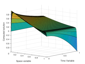
(a) Entire domain $\bar{Q}$

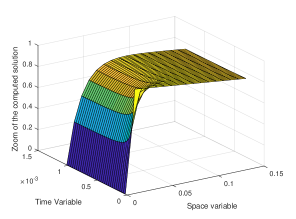
(b) A zoom in on the corner $(0,0)$

Figure 1: Example (26): The numerical approximation to the solution $u$ with $\varepsilon=2^{-12}$ and $N=M=64$

The orders of convergence of the finite difference scheme (14) are estimated using the two-mesh principle [2]. We denote by $Y^{N,M}$ and $Y^{2N,2M}$ the computed solutions with (14) on the Shishkin meshes $Q^{N,M}$ and $Q^{2N,2M}$, respectively. These solutions are used to computed the maximum two-mesh global differences

$$D^{N,M}_{\varepsilon}:=\|\bar{Y}^{N,M}-\bar{Y}^{2N,2M}\|_{Q^{N,M}\cup Q^{2N,2M}}$$

where $\bar{Y}^{N,M}$ and $\bar{Y}^{2N,2M}$ denote the bilinear interpolation of the discrete solutions $Y^{N,M}$ and $Y^{2N,2M}$ on the mesh $Q^{N,M}\cup Q^{2N,2M}$. Then, the orders of global convergence $Q^{N,M}_{\varepsilon}$ are estimated in a standard way [2]

$$Q^{N,M}_{\varepsilon}:=\log_{2}\left(\frac{D^{N,M}_{\varepsilon}}{D^{2N,2M}_{\varepsilon}}\right).$$

The uniform two-mesh global differences $D^{N,M}$ and their corresponding uniform orders of global convergence $Q^{N,M}$ are calculated by

$$D^{N,M}:=\max_{\varepsilon\in S}D^{N,M}_{\varepsilon},\quad Q^{N,M}:=\log_{2}\left(\frac{D^{N,M}}{D^{2N,2M}}\right),$$

where $S=\{2^{0},2^{-1},\ldots,2^{-30}\}$. This is a sufficiently large set of values for the singular perturbation parameter $\varepsilon$ to view the uniform convergence of the scheme (14).

The maximum two-mesh global differences $D^{N,M}_{\varepsilon}$ and the orders of global convergence $Q^{N,M}_{\varepsilon}$ associated with the problem (27) are displayed in Table 1. The uniform two-mesh global differences $D^{N,M}$ and their orders of convergence $Q^{N,M}$ are given in the last row of this table. These numerical results are in line with the error estimate (25) showing that the method is an almost first-order uniformly global convergent scheme.

Table 1: Example (26): Maximum and uniform two-mesh global differences and orders of global convergence associated with the solution $y$ of problem (27)

	N=64	N=128	N=256	N=512	N=1024	N=2048	N=4096
	M=16	M=32	M=64	M=128	M=256	M=512	M=1024
$\varepsilon=2^{0}$	3.287E-03	1.822E-03	9.570E-04	4.893E-04	2.467E-04	1.237E-04	6.192E-05
	0.851	0.929	0.968	0.988	0.996	0.999
$\varepsilon=2^{-1}$	5.854E-03	3.435E-03	1.860E-03	9.647E-04	4.899E-04	2.466E-04	1.236E-04
	0.769	0.885	0.947	0.978	0.991	0.996
$\varepsilon=2^{-2}$	9.217E-03	6.107E-03	3.510E-03	1.875E-03	9.660E-04	4.896E-04	2.464E-04
	0.594	0.799	0.905	0.957	0.980	0.991
$\varepsilon=2^{-3}$	1.266E-02	8.951E-03	6.250E-03	3.540E-03	1.877E-03	9.654E-04	4.892E-04
	0.500	0.518	0.820	0.915	0.960	0.981
$\varepsilon=2^{-4}$	1.266E-02	9.162E-03	6.499E-03	4.197E-03	2.545E-03	1.481E-03	8.388E-04
	0.466	0.495	0.631	0.722	0.781	0.820
$\varepsilon=2^{-5}$	2.200E-02	9.263E-03	6.521E-03	4.199E-03	2.544E-03	1.480E-03	8.384E-04
	1.248	0.506	0.635	0.723	0.781	0.820
$\varepsilon=2^{-6}$	2.990E-02	1.127E-02	6.530E-03	4.199E-03	2.543E-03	1.480E-03	8.382E-04
	1.408	0.787	0.637	0.723	0.781	0.820
$\varepsilon=2^{-7}$	3.123E-02	1.499E-02	6.551E-03	4.204E-03	2.543E-03	1.480E-03	8.382E-04
	1.058	1.194	0.640	0.725	0.781	0.820
$\varepsilon=2^{-8}$	3.125E-02	1.561E-02	7.510E-03	4.218E-03	2.547E-03	1.480E-03	8.382E-04
	1.001	1.056	0.832	0.728	0.783	0.821
$\varepsilon=2^{-9}$	4.082E-02	1.562E-02	7.807E-03	4.245E-03	2.550E-03	1.482E-03	8.388E-04
	1.386	1.001	0.879	0.735	0.783	0.821
$\varepsilon=2^{-10}$	7.276E-02	2.209E-02	7.812E-03	4.299E-03	2.569E-03	1.486E-03	8.397E-04
	1.720	1.499	0.862	0.743	0.790	0.824
$\varepsilon=2^{-11}$	7.349E-02	3.025E-02	1.121E-02	4.426E-03	2.582E-03	1.490E-03	8.410E-04
	1.281	1.432	1.341	0.778	0.793	0.825
$\varepsilon=2^{-12}$	7.352E-02	3.025E-02	1.099E-02	4.372E-03	2.611E-03	1.497E-03	8.446E-04
	1.281	1.461	1.330	0.743	0.803	0.826
$\varepsilon=2^{-13}$	7.354E-02	3.026E-02	1.099E-02	4.372E-03	2.611E-03	1.503E-03	8.428E-04
	1.281	1.461	1.330	0.743	0.797	0.835
	.	.	.	.	.	.	.
	.	.	.	.	.	.	.
	.	.	.	.	.	.	.
$\varepsilon=2^{-29}$	7.360E-02	3.027E-02	1.100E-02	4.372E-03	2.611E-03	1.503E-03	8.428E-04
	1.282	1.461	1.331	0.743	0.797	0.835
$\varepsilon=2^{-30}$	7.360E-02	3.027E-02	1.100E-02	4.372E-03	2.611E-03	1.503E-03	8.428E-04
	1.282	1.461	1.331	0.743	0.797	0.835
$D^{N,M}$	7.360E-02	3.027E-02	1.121E-02	4.426E-03	2.611E-03	1.503E-03	8.446E-04
$Q^{N,M}$	1.282	1.433	1.341	0.761	0.797	0.832

Finally, we give some information about the distribution of the errors. In Figure 2 we display the two-mesh nodal differences $|(Y^{N,M}-\bar{Y}^{2N,2M})(x_{i},t_{j})|$ with $(x_{i},t_{j})\in Q^{N,M}$; and it is observed that the largest differences occur within the layers and, within the initial layer, the maximum two-mesh differences occur at the earlier times.

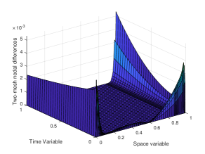
(a) Entire domain $\bar{Q}$

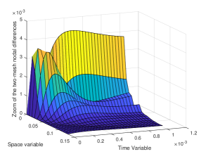
(b) A zoom in on the corner $(0,0)$

Figure 2: Example (26): Two-mesh nodal differences $Y^{N}-Y^{2N}$ for problem (27) on the coarsest mesh $\bar{\Omega}^{N,M}$ with $\varepsilon=2^{-12}$ and $N=M=64$

Appendix 1: Compatibility conditions

In this Appendix, we explicitly write down the compatibility conditions (see e.g. [7, 12]) of zero, first and second order associated with a singularly perturbed parabolic problem in one space dimension. Consider the following problem: Find $s(x,t)$ such that

$$Ls=\varepsilon(s_{t}-s_{xx})+b(x,t)s=g(x,t),\quad(x,t)\in Q,$$ (28a)

$$s(0,t)=g_{L}(t),\ s(1,t)=g_{R}(t)\ t\geq 0,\quad s(x,0)=\phi(x),\ 0<x<1.$$ (28b)

Below we place certain regularity and compatibility restrictions on the data in order that the solution $s\in C^{n+\gamma}(\overline{Q}),\ n=2,4$.

Level zero-order compatibility conditions corresponds to:

$$\phi(0^{+})=g_{L}(0)\quad\hbox{and}\quad\phi(1^{-})=g_{R}(0).$$ (29a)

Assuming (29a), we can write

$$s(x,t) = \Phi(x,t)+z(x,t),\quad(x,t)\in Q\quad\hbox{where}$$

$$\Phi(x,t) := \phi(x)+(1-x)(g_{L}(t)-g_{L}(0))+x\bigl{(}g_{R}(t)-g_{R}(0)\bigr{)};$$

$$Lz=g-L\Phi; z(x,t)=0,\ (x,t)\in\partial Q$$ and . Note that

$$L\Phi=\varepsilon\Bigl{(}(1-x)g_{L}^{\prime}(t)+xg^{\prime}_{R}(t)-\phi^{\prime\prime}(x)\Bigr{)}+b(x,t)\Phi.$$

From [12], if $$b,g,L\Phi\in C^{0+\gamma}(\bar{Q})$$ and the first-order compatibility conditions

$$\varepsilon(g_{R}^{\prime}(0)-\phi^{\prime\prime}(1^{-}))+b(1,0)\phi(1^{-})=g(1,0)$$ (29b)

$$\varepsilon(g^{\prime}_{L}(0)-\phi^{\prime\prime}(0^{+}))+b(0,0)\phi(0^{+})=g(0,0)$$ (29c)

are satisfied, then $$s\in C^{2+\gamma}(\bar{Q}) b,g,L\Phi\in C^{2+\gamma}(\bar{Q})$$. If and we further assume second-order compatibility conditions such that

$$(g-L\Phi)_{t}(0,0^{+})+(g-L\Phi)_{xx}(0^{+},0)=0;$$ (29d)

$$(g-L\Phi)_{t}(1,0^{+})+(g-L\Phi)_{xx}(1^{-},0)=0;$$ (29e)

then the solution of (28) $$s\in C^{4+\gamma}(\bar{Q})$$. Note that the constraint (29d) corresponds to

$$(g_{t}+g_{xx})(0,0) =\varepsilon g^{\prime\prime}_{L}(0^{+})+b(0,0)g^{\prime}_{L}(0^{+})+b_{t}(0,0)g_{L}(0^{+})-\varepsilon\phi^{iv}(0^{+})$$

$$+2b_{x}(0,0)\phi^{\prime}(0^{+})+b_{xx}(0,0)\phi(0^{+})+b(0,0)\phi^{\prime\prime}(0^{+}).$$

Appendix 2: Regularity of the function $y_{2}$

Consider the solutions $z_{n}(x,t),n\geq 0$ of the following problems:

$$\frac{\partial z_{n}}{\partial t}-\frac{\partial^{2}z_{n}}{\partial x^{2}}+\frac{b(0,0)}{\varepsilon}z_{n}=0,\quad x>0,t>0$$

$$z_{n}(x,0)=0,\ x\geq 0;\quad z_{n}(0,t)=t^{n}e^{-\frac{b(0,0)t}{\varepsilon}},\ t>0.$$

Note that

$$z_{0}(x,t)=\hbox{erfc}\left(\frac{x}{2\sqrt{t}}\right)e^{-\frac{b(0,0)t}{\varepsilon}};\ \varepsilon\left|\frac{\partial z_{0}}{\partial t}(x,t)\right|\leq C\frac{1}{t}(\varepsilon+t)e^{-\frac{\beta t}{\varepsilon}};$$

and

$$z_{n}=n\int_{s=0}^{t}z_{n-1}(x,s)e^{-\frac{b(0,0)(t-s)}{\varepsilon}}\ ds;\ (z_{n})_{t}+\frac{b(0,0)}{\varepsilon}z_{n}=nz_{n-1},n\geq 1.$$ (30)

Observe that $z_{n}=v_{n}e^{-b(0,0)t/\varepsilon}$ and the functions $\{v_{n}\}_{n=0}^{4}$ are explicitly given in [4, (5), p.538] and we also note that $(v_{n})_{xx}=(v_{n})_{t}=nv_{n-1}$. From a maximum principle, we have the following bounds:

$$|z_{n}(x,t)|\leq t^{n}e^{-\frac{b(0,0)t}{\varepsilon}}\leq C\varepsilon^{n}e^{-\frac{\beta t}{\varepsilon}};\ n=0,1,2.$$ (31)

Let us list some of the derivatives of the fundamental function $z_{0}(x,t)$

$$\frac{\partial z_{0}}{\partial x} = \frac{-1}{\sqrt{\pi t}}e^{-\frac{x^{2}}{4t}}e^{-\frac{b(0,0)t}{\varepsilon}}=O\left(\frac{1}{\sqrt{t}}\right)$$

$$\frac{\partial^{2}z_{0}}{\partial x^{2}} = \frac{\partial z_{0}}{\partial t}+\frac{b(0,0)}{\varepsilon}z_{0}=\frac{x}{2t\sqrt{\pi t}}e^{-\frac{x^{2}}{4t}}e^{-\frac{b(0,0)t}{\varepsilon}}=O\left(\frac{1}{t}\right)$$

$$\frac{\partial^{3}z_{0}}{\partial x^{3}} = \frac{1}{2t\sqrt{\pi t}}(1-\frac{x^{2}}{2t})e^{-\frac{x^{2}}{4t}}e^{-\frac{b(0,0)t}{\varepsilon}}=O\left(\frac{1}{t\sqrt{t}}\right)$$

$$\frac{\partial^{4}z_{0}}{\partial x^{4}} = \frac{\partial^{2}z_{0}}{\partial t^{2}}+2\frac{b(0,0)}{\varepsilon}\frac{\partial z_{0}}{\partial t}+\left(\frac{b(0,0)}{\varepsilon}\right)^{2}z_{0}$$

$$= \frac{-x}{4t^{2}\sqrt{\pi t}}\left(3-\frac{x^{2}}{2t}\right)e^{-\frac{x^{2}}{4t}}e^{-\frac{b(0,0)t}{\varepsilon}}=O\left(\frac{1}{t^{2}}\right)$$

$$\frac{\partial z_{0}}{\partial t}=O\left(\frac{1}{\varepsilon}\right)z_{0}+O\left(\frac{1}{t}\right) \frac{\partial^{2}z_{0}}{\partial t^{2}}=O\left(\frac{1}{\varepsilon^{2}}\right)z_{0}+O\left(\frac{1}{\varepsilon t}\right)+O\left(\frac{1}{t^{2}}\right).$$ ,

Observe that the function

$$h(x,t):=\frac{x}{\sqrt{t}}e^{-\frac{x^{2}}{4t}},\ t>0,\quad h(x,0):=0,\ 0\leq x\leq 1;$$

is bounded, but not continuous on $\bar{Q}$. From this and the explicit expressions for the derivatives of $z_{0}$ given above, we deduce that

$$S_{i,j}(x,t):=x^{i}t^{j}z_{0}\in C^{2+\gamma}(\bar{Q}),\quad i+2j\geq 4$$

and the second derivative in time of these functions $S_{i,j}$, when $i+2j=4$, are all bounded on $\bar{Q}$, but not continuous. Moreover, for $i+2j\geq 4$, we have

$$\Bigl{|}\frac{\partial^{n+m}}{\partial x^{n}\partial t^{m}}(S_{i,j}(x,t))\Bigr{|}\leq C\varepsilon^{-m}e^{-\frac{\beta t}{\varepsilon}},\qquad 0\leq n+2m\leq 4;$$ (32)

and for all integers $m,n\geq 1$

$$L_{0}(t^{n}z_{0}) = \varepsilon nt^{n-1}z_{0};$$

$$L_{0}(t^{n}x^{m}z_{0}) = \varepsilon(x^{m}nt^{n-1}z_{0}-m(m-1)x^{m-2}t^{n}z_{0}-2mx^{m-1}t^{n}(z_{0})_{x}).$$

We identify the following set of functions, $\{\chi_{i,j}\}$,

$$L_{0}\chi_{i,j}=S_{i,j}(x,t);\quad i,j=0,1,2...$$

where the first few functions in the set $\{\chi_{i,j}\}$ are explicitly given as

$$\varepsilon\chi_{1,0} = xtz_{0}+t^{2}(z_{0})_{x}\quad\hbox{and}\quad|\chi_{1,0}(0,t)|\leq C\sqrt{t}e^{-\frac{\beta t}{\varepsilon}};$$ (33a)

$$\varepsilon\chi_{0,1} = \frac{t^{2}z_{0}}{2}\quad\hbox{and}\quad|\chi_{0,1}(0,t)|\leq Cte^{-\frac{\beta t}{\varepsilon}};$$ (33b)

$$\varepsilon\chi_{2,0} = (x^{2}t+t^{2})z_{0}+2xt^{2}(z_{0})_{x}+(4/3)t^{3}(z_{0})_{xx},$$ (33c)

and $$\varepsilon\chi_{2,0}(0,t)=t^{2}e^{-\frac{b(0,0)t}{\varepsilon}};$$

$$\varepsilon\chi_{1,1} = \frac{3xt^{2}z_{0}+2t^{3}(z_{0})_{x}}{6}\ \hbox{and}\ |\chi_{1,1}(0,t)|\leq Ct\sqrt{t}e^{-\frac{\beta t}{\varepsilon}}$$ (33d)

$$\varepsilon\chi_{3,0} = (x^{3}t+3xt^{2})z_{0}+(4t^{3}+3x^{2}t^{2})(z_{0})_{x}+4xt^{3}(z_{0})_{xx}+2t^{4}(z_{0})_{xxx}$$

$$|\chi_{3,0}(0,t)|\leq Ct\sqrt{t}e^{-\frac{\beta t}{\varepsilon}}.$$

Using the recurrence relation (30) and the above properties of $z_{0}$ we have that

$$\left|\frac{\partial^{2}z_{1}}{\partial x^{2}}(x,t)\right|+\left|\frac{\partial z_{1}}{\partial t}(x,t)\right| \leq Ce^{-\frac{\beta t}{\varepsilon}};$$ (34a)

$$\left|\frac{\partial^{3}z_{1}}{\partial x^{3}}(x,t)\right| \leq C\frac{1}{\sqrt{t}}e^{-\frac{x^{2}}{4t}}e^{-\frac{b(0,0)t}{\varepsilon}};$$ (34b)

$$\left|\frac{\partial^{4}z_{1}}{\partial x^{4}}(x,t)\right|+\varepsilon\left|\frac{\partial^{2}z_{1}}{\partial t^{2}}(x,t)\right| \leq C\frac{1}{t}(\varepsilon+t)e^{-\frac{\beta t}{\varepsilon}};$$ (34c)

$$\left|\frac{\partial^{4}z_{2}}{\partial x^{4}}(x,t)\right|+\left|\frac{\partial^{2}z_{2}}{\partial t^{2}}(x,t)\right| \leq Ce^{-\frac{\beta t}{\varepsilon}}.$$ (34d)

Note also that

$$\left|\frac{\partial^{2}z_{0}}{\partial t^{2}}(x,t)\right|\leq\frac{C}{(\varepsilon+t)^{2}}e^{-\frac{b(0,0)t}{\varepsilon}};\ \left|\frac{\partial^{2}z_{1}}{\partial t^{2}}(x,t)\right|\leq\frac{C}{t}e^{-\frac{b(0,0)t}{\varepsilon}};$$

$$\left|\frac{\partial^{2}z_{2}}{\partial t^{2}}(x,t)\right|\leq Ce^{-\frac{b(0,0)t}{\varepsilon}}.$$

Recall that the solution $u$ of problem (1) is discontinuous at the point $(0,0)$ and by subtracting the discontinuous function $A_{0}z_{0}$, we see that $y=u-A_{0}z_{0}$ satisfies zero order compatibility at the point $(0,0)$. Hence the solution $y$ of problem (7) is a continuous function. By subtracted off appropriate multiples $A_{n}$ of $z_{n}$ (see (30)) from $u$ we can satisfy up to the $n^{th}$ order compatibility conditions at the point $(0,0)$. Since $L_{0}z_{n}=0$, one can check that

$$L(u-A_{0}z_{0}),L(u-A_{0}z_{0}-A_{1}z_{1})\in C^{0+\gamma}(\bar{Q})$$

and this implies that $(u-A_{0}z_{0})\in C^{2+\gamma}(\bar{Q})$. Thus $y\in C^{0}(\bar{Q})$ and $(y-A_{1}z_{1})\in C^{2+\gamma}(\bar{Q})$, but $(y-A_{1}z_{1}-A_{2}z_{2})\not\in C^{4+\gamma}(\bar{Q})$. We now define the following two functions

$$y_{1}:=y-A_{1}z_{1}\quad\hbox{and}\quad y_{2}:=y_{1}-A_{2}z_{2}-A_{0}\Psi;$$

where

$$\Psi(x,t):=b_{t}(0,0)\chi_{0,1}+\frac{b_{xx}(0,0)}{2}\chi_{2,0}+b_{xt}(0,0)\chi_{1,1}+\frac{b_{xxx}(0,0)}{6}\chi_{3,0}$$

$$\hbox{and}\quad L_{0}\Psi=\left(b_{t}(0,0)t+\frac{b_{xx}(0,0)}{2}x^{2}+b_{xt}(0,0)xt+\frac{b_{xxx}(0,0)}{6}x^{3}\right)z_{0}.$$

We shall see below that the additional term $A_{0}\Psi$ has been included so that $y_{2}\in C^{4+\gamma}(\bar{Q})$. The amplitude $A_{0}$ has been determined above. Below we specify the amplitudes $A_{1}$ and $A_{2}$. Observe that the function $y_{1}$ satisfies

$$Ly_{1}=f-(b(x,t)-b(0,0))\bigl{(}A_{1}z_{1}+A_{0}z_{0}\bigr{)};$$

$$y_{1}(0,t)=g_{L}(t)-(A_{0}z_{0}+A_{1}z_{1})(0,t);\ y_{1}(1,t)=g_{R}(t)-(A_{0}z_{0}+A_{1}z_{1})(1,t);$$

$$y_{1}(x,0)=\phi(x).$$

From (29c) in the first Appendix, first order compatibility is satisfied (for $y_{1}$) if $A_{1}$ is such that

$$f(0,0)=\varepsilon(g_{L}^{\prime}(0^{+})-A_{1}-\phi_{xx}(0^{+}))+b(0,0)(A_{0}+\phi(0)).$$ (35)

In general, $A_{1}=O(\varepsilon^{-1})$. Since $Ly_{1}\in C^{0+\gamma}(\bar{Q})$, then $y_{1}\in C^{2+\gamma}(\bar{Q})$.

Next we move onto the regularity of $y_{2}$. Note first that, since $b_{x}(0,0)=0$,

$$(L-L_{0})z_{n}=\left(b_{t}(0,0)t+\frac{b_{xx}(0,0)}{2}x^{2}+b_{xt}(0,0)xt+\frac{b_{xxx}(0,0)}{6}x^{3}\right)z_{n}+\ \hbox{H.O.T.}.$$

Hence,

$$Ly_{2} = Ly_{1}-(L-L_{0})(A_{2}z_{2}+A_{0}\Psi)-A_{0}L_{0}\Psi$$

$$= f-(L-L_{0})\bigl{(}A_{1}z_{1}+A_{0}z_{0}\bigr{)}-A_{0}L_{0}\Psi-(b(x,t)-b(0,0))(A_{2}z_{2}+A_{0}\Psi)$$

$$= f+O(t^{2}+x^{4}+x^{2}t)A_{0}z_{0}-(L-L_{0})\bigl{(}A_{1}z_{1}\bigr{)}-(b(x,t)-b(0,0))(A_{2}z_{2}+A_{0}\Psi)$$

$$= f+O(t^{2}+x^{4}+x^{2}t)A_{0}z_{0}+O(t+x^{2})A_{2}z_{2}+O(t+x^{2})A_{1}z_{1};$$

$$+\varepsilon^{-1}A_{0}O(t+x^{2})\bigl{(}O(x^{2}t+t^{2})z_{0}+O(xt^{2}+t^{3})(z_{0})_{x}+O(t^{3})(z_{0})_{xx}+O(t^{4})(z_{0})_{xxx}\bigr{)}$$

and the boundary and initial conditions are

$$y_{2}(0,t)=g_{L}(t)-\bigl{(}A_{0}z_{0}+A_{1}z_{1}+A_{2}z_{2}+A_{0}\Psi\bigr{)}(0,t)$$

$$=g_{L}(t)-\left(A_{0}+A_{1}t+A_{2}t^{2}\right)e^{-\frac{b(0,0)t}{\varepsilon}}-A_{0}\frac{t^{2}}{2\varepsilon}b_{t}(0,0)e^{-\frac{b(0,0)t}{\varepsilon}}$$

$$-A_{0}\frac{t^{2}}{2\varepsilon}\left(b_{xx}(0,0)\left(z_{0}+\frac{4t}{3}\frac{\partial^{2}z_{0}}{\partial x^{2}}\right)+\frac{2b_{xt}(0,0)t}{3}\frac{\partial z_{0}}{\partial x}+\frac{2b_{xxx}(0,0)}{3}\left(2t\frac{\partial z_{0}}{\partial x}+t^{2}\frac{\partial^{3}z_{0}}{\partial x^{3}}\right)\right)(0,t);$$

$$y_{2}(1,t)=y(1,t)-\bigl{(}A_{1}z_{1}+A_{2}z_{2}+A_{0}\Psi\bigr{)}(1,t);\quad y_{2}(x,0)=\phi(x).$$

Note that $\lim_{t\rightarrow 0^{+}}y_{2}(0,t)=g_{L}(0^{+})-A_{0}$ and

$$\lim_{t\rightarrow 0^{+}}\frac{\partial y_{2}(0,t)}{\partial t} =g^{\prime}_{L}(0^{+})-A_{1}+A_{0}\frac{b(0.0)}{\varepsilon}$$

$$\lim_{t\rightarrow 0^{+}}\frac{\partial^{2}y_{2}(0,t)}{\partial t^{2}} =g^{\prime\prime}_{L}(0^{+})+2\varepsilon^{-1}A_{1}b(0,0)-2A_{2}-2\varepsilon^{-1}A_{0}(b_{t}(0,0)+b_{xx}(0,0))$$

$$-A_{0}(\frac{b(0,0)}{\varepsilon})^{2}.$$

First order compatibility is satisfied (for $y_{2}$) if $A_{1}$ is such that (35) is satisfied and the above construction has been designed in order that $Ly_{2}\in C^{2+\gamma}(\bar{Q})$. Finally second order compatibility is satisfied (for $y_{2}$) if $A_{2}$ is such that

$$\varepsilon(g_{L}^{\prime\prime}(0^{+})-\phi^{iv}(0^{+}))+(A_{1}+g^{\prime}_{L}(0^{+}))b(0,0)-2\varepsilon A_{2}-2A_{0}(b_{t}(0,0)+b_{xx}(0,0))$$

$$-A_{0}\varepsilon^{-1}b^{2}(0,0)+b_{t}(0,0)(g_{L}(0)-A_{0})+b_{xx}(0,0)\phi(0^{-})+b(0,0)\phi^{\prime\prime}(0^{+})$$

$$\quad=\bigl{(}f_{t}+f_{xx}\bigr{)}(0,0).$$ (36)

Note that $A_{0}=O(1),\quad A_{1}=O(\varepsilon^{-1})\quad\hbox{and}\quad A_{2}=O(\varepsilon^{-2}).$ By this construction we have that $y_{2}\in C^{4+\gamma}(\bar{Q})$. Moreover,

$$\Bigl{|}\frac{\partial^{i+j}}{\partial x^{i}\partial t^{j}}(Ly_{2}(x,t))\Bigr{|}\leq C\varepsilon^{-j}e^{-\frac{\beta t}{\varepsilon}},\quad 0\leq i+2j\leq 2.$$ (37)

References

• [1] Q. Chen, Z. Qin and R. Temam, Treatment of incompatible initial and boundary data for parabolic equations in higher dimensions, Math. Comp., 80, 276, 2011, 2071–2096.
• [2] P.A. Farrell, A.F. Hegarty, J.J.H. Miller, E. O’Riordan and G.I. Shishkin, Robust computational techniques for boundary layers, CRC Press, 2000.
• [3] M. Fei, D. Han and X. Wang, Initial-boundary layer associated with the nonlinear Darcy-Brinkman-Oberbeck-Boussinesq system, Phys. D, 338, 2017, 42–56.
• [4] N. Flyer and B. Fornberg, Accurate numerical resolution of transients in initial-boundary value problems for the heat equation, J. Comp. Physics 184, 2003, 526–539.
• [5] J.L. Gracia and E. O’Riordan, A singularly perturbed reaction-diffusion problem with incompatible boundary-initial data, Lecture Notes in Computer Science, I. Dimov, I. Farago, and L. Vulkov (Eds.): Numerical Analysis and Its Applications: 5th Int. Conf., NAA 2012, Lozenetz, Bulgaria, v. 8236, 303–310. Springer (2013).
• [6] J.L. Gracia and E. O’Riordan, A singularly perturbed parabolic problem with a layer in the initial condition, Appl. Math. Comp. 219, 2012, 498–510.
• [7] A. Friedman, Partial differential equations of parabolic type, Prentice-Hall, Englewood Cliffs, N.J., (1964).
• [8] D. Han and X. Wang, Initial-boundary layer associated with the nonlinear Darcy-Brinkman system, J. Differential Equations, 256, (2), 2014, 609–639.
• [9] P.W. Hemker and G.I. Shishkin, Approximation of parabolic PDEs with a discontinuous initial condition, East-West J. Numer. Math, 1, 1993, 287–302.
• [10] P.W. Hemker and G.I. Shishkin, Discrete approximation of singularly perturbed parabolic PDEs with a discontinuous initial condition, Comp. Fluid Dynamics J, 2, 1994, 375–392.
• [11] N.V. Kopteva and E. O’Riordan, Shishkin meshes in the numerical solution of singularly perturbed differential equations, Int. J. Numer. Anal. Model., 7, 2010, 393–415.
• [12] O.A. Ladyzhenskaya, V.A. Solonnikov and N.N. Ural’tseva, Linear and quasilinear equations of parabolic type, Transactions of Mathematical Monographs, 23, American Mathematical Society, (1968).
• [13] J.J.H. Miller and E. O’Riordan, The necessity of fitted operators and Shishkin meshes for resolving thin layer phenomena, CWI Quarterly, 10, 207–213, 1997.
• [14] J.J.H. Miller, E. O’Riordan, G.I. Shishkin and L.P. Shishkina, Fitted mesh methods for problems with parabolic boundary layers, Mathematical Proceedings of the Royal Irish Academy, 98A, 1998, 173–190.
• [15] J.J.H. Miller, E. O’Riordan and G.I. Shishkin, Fitted Numerical Methods for Singular Perturbation Problems, World-Scientific, Singapore (Revised edition), 2012.
• [16] E. O’Riordan and G. I. Shishkin, Parameter uniform numerical methods for singularly perturbed elliptic problems with parabolic boundary layers, Applied Numerical Mathematics, 58, 2008, 1761-1772.
• [17] M. Stynes and E. O‘Riordan, Uniformly convergent difference schemes for singularly perturbed parabolic diffusion-convection problems without turning points, Numer. Math., 55, 1989, 521–544.
• [18] U.Kh. Zhemukhov, Parameter-uniform error estimate for the implicit four-point scheme for a singularly perturbed heat equation with corner singularities. Translation of Differ. Uravn. 50 (2014), 7, 923–-936. Differ. Equ. 50 (2014), 7, 913–926.
• [19] U.Kh. Zhemukhov, On the convergence of the numerical solution of an initial-boundary value problem for the heat equation in the presence of a corner singularity in the derivatives of the solution. (in Russian) Vestnik Moskov. Univ. Ser. XV Vychisl. Mat. Kibernet. 2013, 4, 9–18, 50; translation in Moscow Univ. Comput. Math. Cybernet. 37 (2013),4, 162–171.