On limiting characteristics for a non-stationary two-processor heterogeneous system
A. Zeifman111Vologda State University; Institute of Informatics
Problems, Federal Research Center ”Informatics and Control” of RAS; Vologda Research Center of RAS; zeifman@mail.ru, Y. Satin222Vologda State University, K. Kiseleva333Vologda State University, T. Panfilova444Vologda State University, V. Korolev555Faculty of
Computational Mathematics and Cybernetics, Lomonosov Moscow State
University; Institute of Informatics Problems, Federal Research
Center ”Informatics and Control” of RAS
1 Introduction
In this paper we study a non-stationary Markovian queueing model of
a two-processor heterogeneous system with time-varying arrival and
service rates which was firstly investigated in [21], see
also time-dependent analysis of this model in the recent paper
[20]. In general, non-stationary queueing models have been
actively studied during some decades, see, for instance
[3, 5, 6, 11, 16, 18]
and the references therein.
In the paper [20] the authors deal with the so-called
“time-dependent analysis”, in other words, they try to find the
state probabilities on a finite interval under some initial
conditions (as a rule, initially, the number of customers in the
queue is zero), see for instance [2]. Another
approach is connected with the determination of the limiting mode,
see [1].
Essentially more information about queue-length process can be
obtained using ergodicity and the corresponding estimates of the
rate of convergence. A general approach to obtaining sharp bounds on
the rate of convergence via the notion of the logarithmic norm of an
operator function wsa recently discussed in details in our papers
[23, 24, 25]. The first
studies in this direction were published since 1980-s for
birth-death models, see [14, 15]. In
[23] we proved that there are four classes of
Markovian queueing models for which the reduced forward Kolmogorov
system can be transformed to the system with essentially nonnegative
matrix. Although the model under consideration does not belong to
one of these classes, we can apply the same approach and obtain some
useful bounds on the rate of convergence for it. Moreover, we can
compute the limiting characteristics of the model using bounds on
the rate of convergence and truncations technique introduced in
[17, 22].
Note an interesting fact: exact estimates of the rate of convergence
yield exact estimates of stability (perturbation bounds), see
[7, 8, 9, 10, 13, 19]
and references therein.
An important feature of multiprocessor queueing systems is the
presence of risks related to the overload of the system. In the
present paper it is demonstrated that under natural conditions on
the arrival/service rates these risks vanish and the system rather
easily approaches the ergodic mode.
2 Description of the model
Here we consider a multiprocessor system consisting of two types of
processors, which for convenience will be referred to as the
“main” and “backup” processors [20]. Each job requires
exactly one processor for its execution. When both processors are
idle, the main processor is scheduled for service before the backup
processor. A computer system consists of two processors, a main
processor, and a backup processor. A description of the model is as
follows:
(i) jobs arrive at the system according to the Poisson
process with an arrival rate . Service is exponentially
distributed, and two servers provide heterogeneous service rates
such that .
(ii) each job needs only one server to be served and the
jobs select the servers on the basis of fastest server first (FSF).
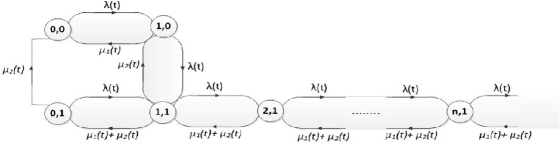
Figure 1: Transitions for a two-processor heterogeneous model
The probabilistic dynamics of the process is represented by the
forward Kolmogorov system of differential equations:
(1)
where
(2)
where , and - the intensity matrix.
3 Bounds on the rate of convergence
Since due
to the normalization condition, the system (1) can be
rewritten as
(3)
where
and
(4)
Denote by the upper triangular matrix
(5)
Consider the matrix
(6)
Let , , be a sequence of positive numbers such
that
Let be the corresponding
diagonal matrix and be a space of vectors
where
Consider the matrix
(7)
The approach used in this paper is based on the notion of the
logarithmic norm of a linear operator function and the corresponding
bounds of the Cauchy operator, see the detailed discussion, for
instance, in [4]. Namely, if , , is a one-parameter family of bounded linear operators on a
Banach space , then
(8)
is called the logarithmic norm of the operator .
If , then the operator is given by
the matrix , , and the logarithmic norm of
can be found explicitly:
(9)
Hence the following bound on the rate of convergence holds:
where and is the solution of the
differential equation
Let be negative sums of the elements of corresponding
columns for the matrix (7), such as:
where since
.
Then we obtain the logarithmic norm:
(10)
4 The case .
First, let be constant,
Then the exact value of the decay parameter
(or the spectral gap) for a simple birth-death process with
intensities and is well-known, namely, it equals
see, e. g., [12],
and the corresponding . Hence, we
consider the same and put
.
Then
Put Then we have
(11)
Hence the following bound holds:
(12)
Let now the intensities be 1-periodic.
Put
Then the best possible bound for a pure birth-death process is
attained, if we take
Then for these , we
have
(13)
(14)
(15)
(16)
Put We
have
(17)
Hence the following bound holds:
(18)
Remark 1. It should be noted that in [20] there are
some misprints in the plots, namely, the intensities must have a
multiplier , say . Moreover, on Fig 3 of that
paper the sum of all probabilities evidently is greater than 1.
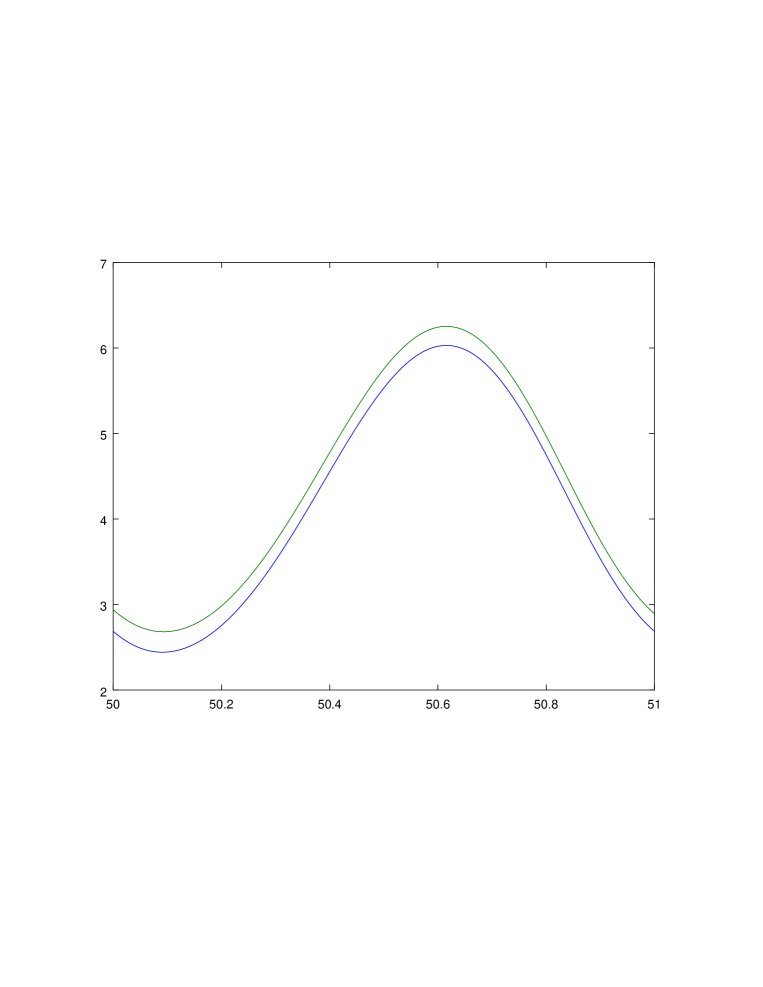
Remark 2. It can be seen that actually the periodic terms in
the intensities do not affect the rate of convergence, see the plots
related to the examples. Hence it is essentially easier to find the
parameter for the corresponding homogeneous model.
Namely, if we put
(19)
(20)
instead of (13)-(16), then we obtain
and the bound on the rate of convergence in the form
(21)
for some positive N.
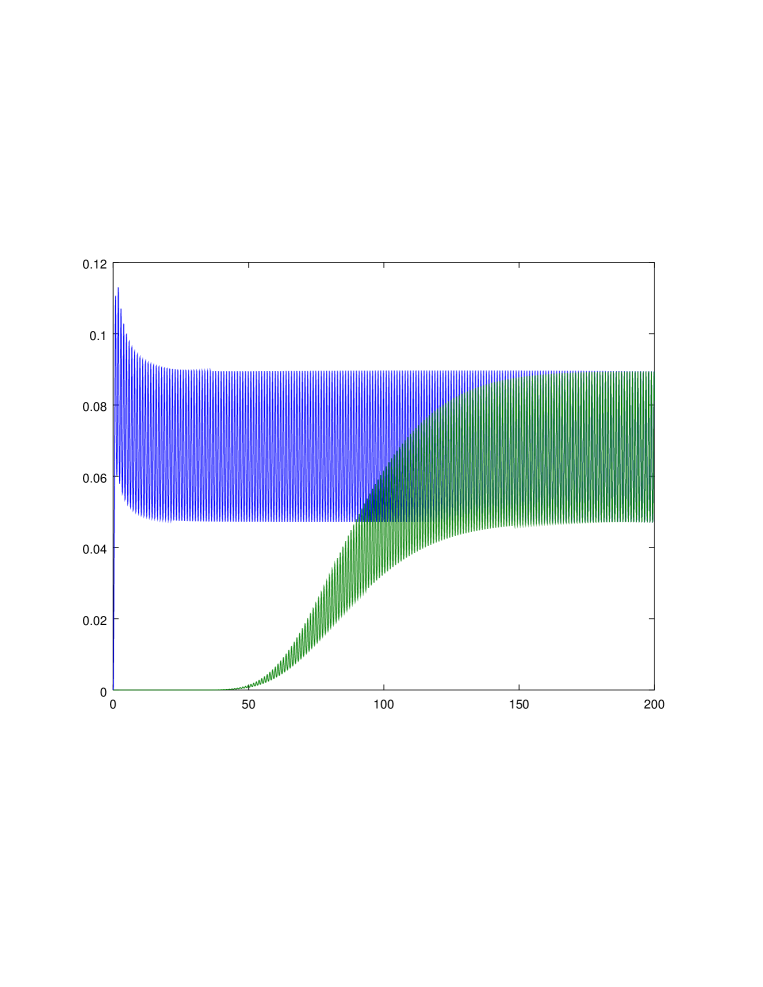
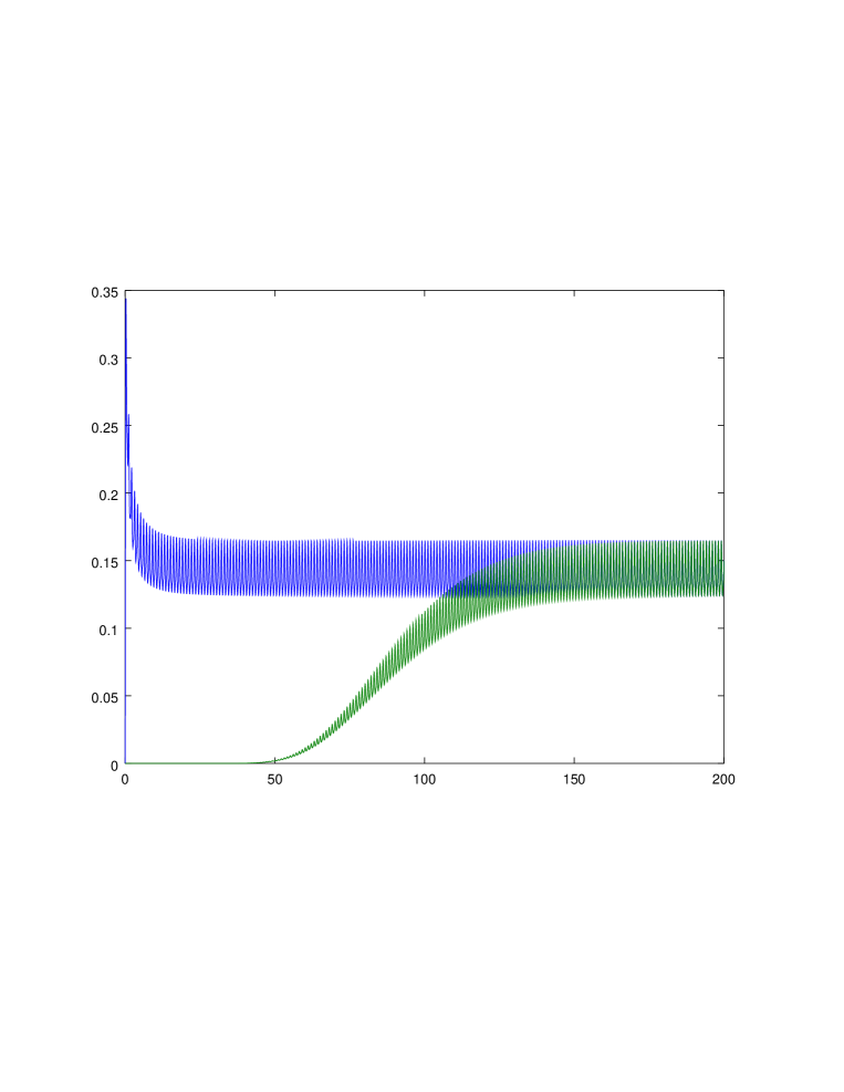
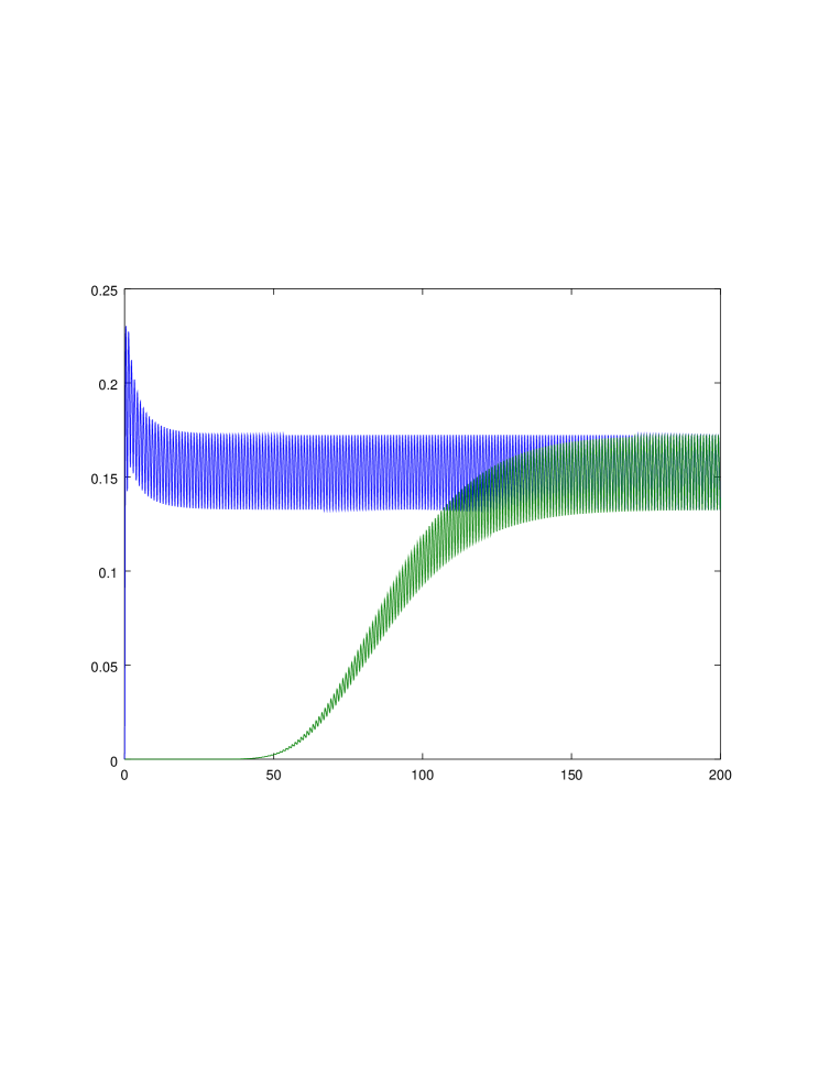
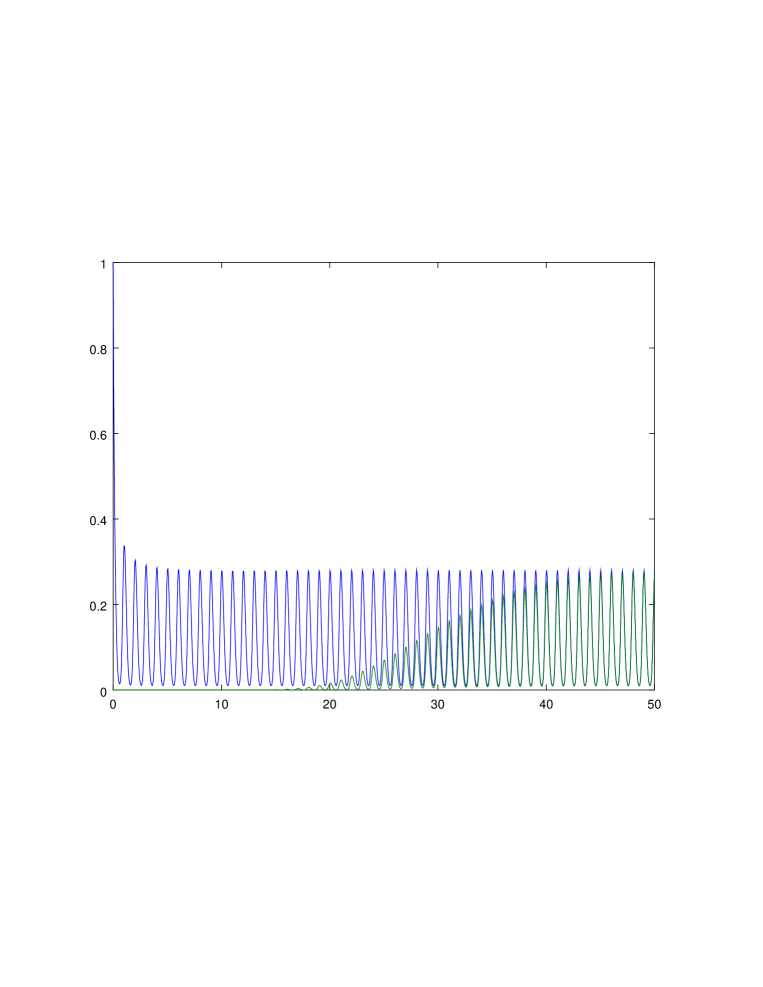
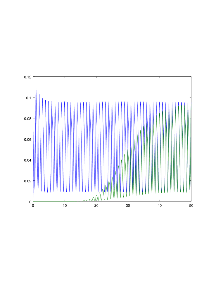
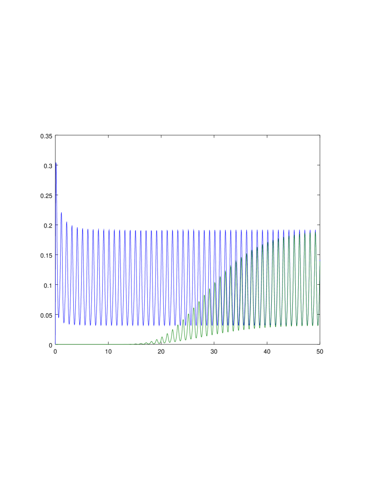
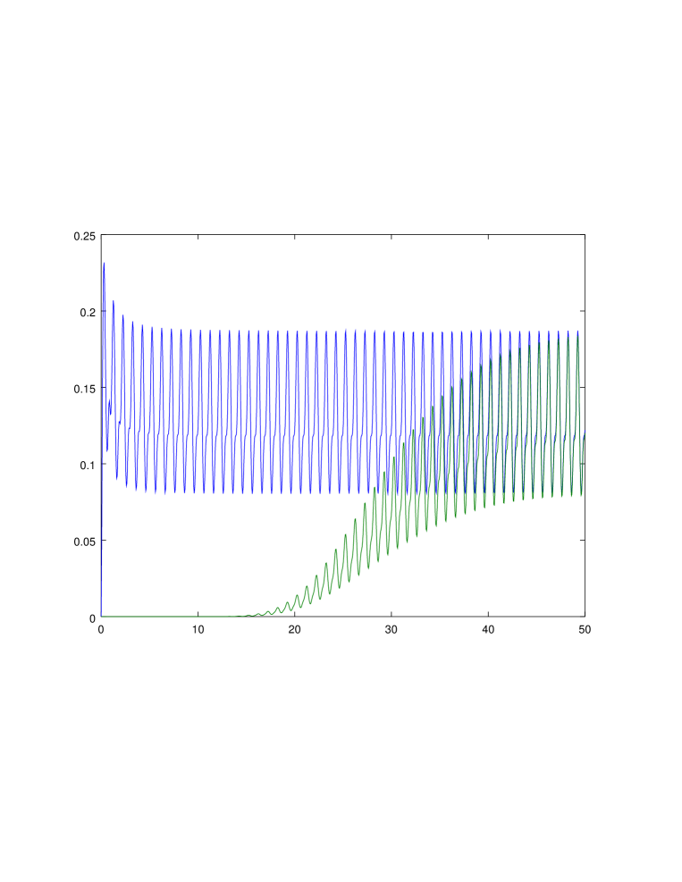
Remark 3. In the following examples we consider the behavior
of the ’first’ state probabilities , ,
, , , and the
mathematical expectation (the mean) of the queue-length process
. One can see that for all examples the rates of convergence for original model with
periodic intensities and for the corresponding homogeneous model
are the same, as it was noted in Remark 2.
5 Examples
Example 1. Let
(Example 2 from [20]). Put
. Then we obtain
for sufficiently small . Therefore, we have . Thus, we can obtain the following bound
On the other hand, we can obtain a simpler bound by applying Remark
2. Namely, , , , , and
Now, applying our standard truncations technique, see the detailed
discussion and bounds in [17, 22], we can
find the limiting characteristics of the queue-length process, the
respective plots are shown in pictures X-Y.
Example 2. Let (Example 3 from [20]). Put
. Then we obtain
, ,
On the other hand, using Remark 2 we have simple corresponding
bounds: , ,
. Hence
Thus we can obtain the following bound
6 The case .
First, let the intensities be constant. Put
, where for Then we have
and
Put Then we have
(22)
Hence, the following bound on the rate of convergence holds:
(23)
Let now the intensities , be
1-periodic. Put
Then, in accordance with Remark 2, we can find the corresponding
parameter for the respective homogeneous model. Namely,
we have and the
bound on the rate of convergence (21) for some positive
N.
Example 3. Let ,
, . (Example 1 from [20]). Then ,
, , Hence, we have
and
As we have already noted, the best value of the bound is attained,
when , then
Now put and . Then
, , and
.
Then we obtain
and the
following bound on the rate of convergence holds:
Acknowledgments.
The bounds on the rate of
convergence have been obtained by Zeifman and Korolev. The work of
Zeifman and Korolev is supported by the Russian Science Foundation
under grant 18-11-00155. Examples have been studied by Satin,
Kiseleva, Panfilova.
References
[1] Chakravarthy, S. R. 2017. A catastrophic queueing model
with delayed action. Applied Mathematical Modelling, 46, 631–649.
[2] Di Crescenzo, A., Giorno, V., Nobile, A. G. 2016.
Constructing transient birth death processes by means of suitable
transformations. Applied Mathematics and Computation, 281, 152–171.
[3] Dong, J., Whitt, W. (2015). Stochastic grey-box modeling of
queueing systems: fitting birth-and-death processes to data.
Queueing Systems, 79(3-4), 391-426.
[4] Van Doorn, E. A., Zeifman, A. I., Panfilova, T. L. Bounds and asymptotics for the rate of convergence of birth-death processes. Th. Probab. Appl. 54, 97–113 (2010)
[5]
Giorno, V., Nobile, A. G., Spina, S. On some time non-homogeneous queueing systems with catastrophes. Appl. Math. Comp. 245, 220–234 (2014)
[6] Granovsky, B. L., Zeifman, A. (2004). Nonstationary queues:
estimation of the rate of convergence. Queueing Systems, 46(3-4),
363–388.
[7] Kartashov, N. V. Criteria for uniform ergodicity and strong stability of Markov chains with a common phase space. Theory
[8] Liu, Y. (2012). Perturbation bounds for the stationary distributions
of Markov chains. SIAM Journal on Matrix Analysis and Applications,
33(4), 1057-1074.
[9] Mitrophanov, A. Yu. Stability and exponential convergence of continuous-time Markov chains.
[10] Mitrophanov, A. Yu. The spectral gap and
perturbation bounds for reversible continuous-time Markov chains.
J. Appl. Probab. 41, 1219–1222 (2004)
[11] Schwarz, J. A., Selinka, G., Stolletz, R. (2016). Performance
analysis of time-dependent queueing systems: survey and
classification. Omega, 63, 170-189.
[12] Van Doorn, E. A. (1985). Conditions for exponential ergodicity and bounds for the decay parameter of a birth-death process. Advances in Applied Probability, 17(3), 514-530.
[13] Zeifman, A. I. (1985). Stability for continuous-time nonhomogeneous
Markov chains. In Stability problems for stochastic models (pp.
401-414). Springer, Berlin, Heidelberg.
[14] Zeifman, A. I. Some properties of a system with losses in the case of variable
rates. Autom. Remote Contr. 50:1, 82 -87 (1989)
[15] Zeifman, A. I. Upper and lower bounds on the rate of
convergence for nonhomogeneous birth and death processes. Stoch.
Proc. Appl. 59, 157–173 (1995)
[16] Zeifman, A., Leorato, S., Orsingher, E., Satin, Y., Shilova, G.
(2006). Some universal limits for nonhomogeneous birth and death
processes. Queueing systems, 52(2), 139-151.
[17] Zeifman, A., Satin, Ya., Korolev, V., Shorgin, S. On truncations for weakly ergodic
inhomogeneous birth and death processes. Int. J. Appl. Math. Comp. Sci. 24, 503–518 (2014)
[18] Zeifman, A., Korotysheva, A. , Korolev, V., Satin, Y., Bening, V.
Perturbation bounds and truncations for a class of Markovian queues. Queueing Syst. 76, 205–221 (2014)
[19] Zeifman, A. I., Korolev, V. Y. On perturbation bounds for
continuous-time Markov chains. Stat. Probab. Lett. 88, 66–72 (2014)
[20] Ammar, S. I., Alharbi, Y. F. (2018). Time-dependent
analysis for a two-processor heterogeneous system with time-varying
arrival and service rates. Applied Mathematical Modelling, 54,
743-751.
[21] S. Dharmaraja, Transient solution of a two-processor heterogeneous system, Math. Comput. Model. 32 (2000), 1117- 1123.
[22] Zeifman, A. I.; Korotysheva, A. V.; Korolev, V. Yu.; Satin Ya. A.
Truncation bounds for approximations of inhomogeneous
continuous-time Markov chains. Th. Prob. Appl. 2016, 61,
563–569.
[23] A. Zeifman, R. Razumchik, Y. Satin, K.
Kiseleva, A. Korotysheva, V. Korolev. Bounds on the rate of
convergence for one class of inhomogeneous Markovian queueing models
with possible batch arrivals and services. Int. J. Appl. Math. Comp.
Sci. 28, (2018)
[24] A. Zeifman, A. Sipin, V. Korolev, G. Shilova, K. Kiseleva, A. Korotysheva, Y. Satin. On Sharp Bounds on the Rate of Convergence
for
Finite Continuous-time Markovian Queueing Models, LNCS 2018
[25] Zeifman, A. I., Korolev, V. Y., Satin, Y. A., Kiseleva, K. M.
(2018). Lower bounds for the rate of convergence for continuous-time
inhomogeneous Markov chains with a finite state space. Statistics &
Probability Letters, 137, 84–90.
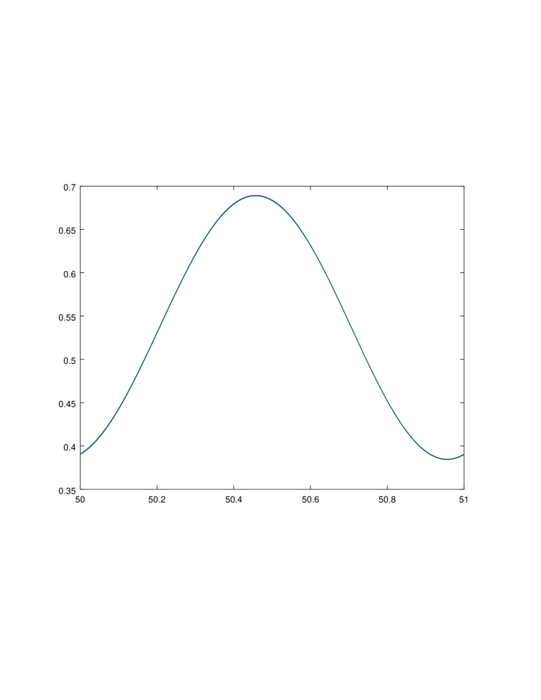
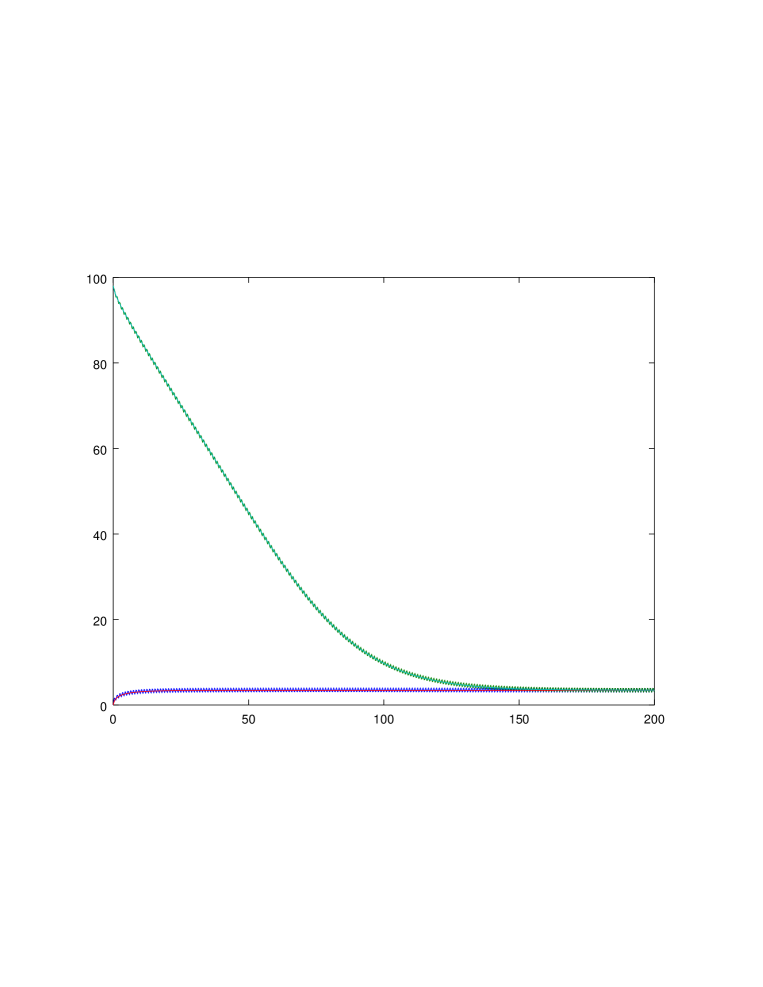
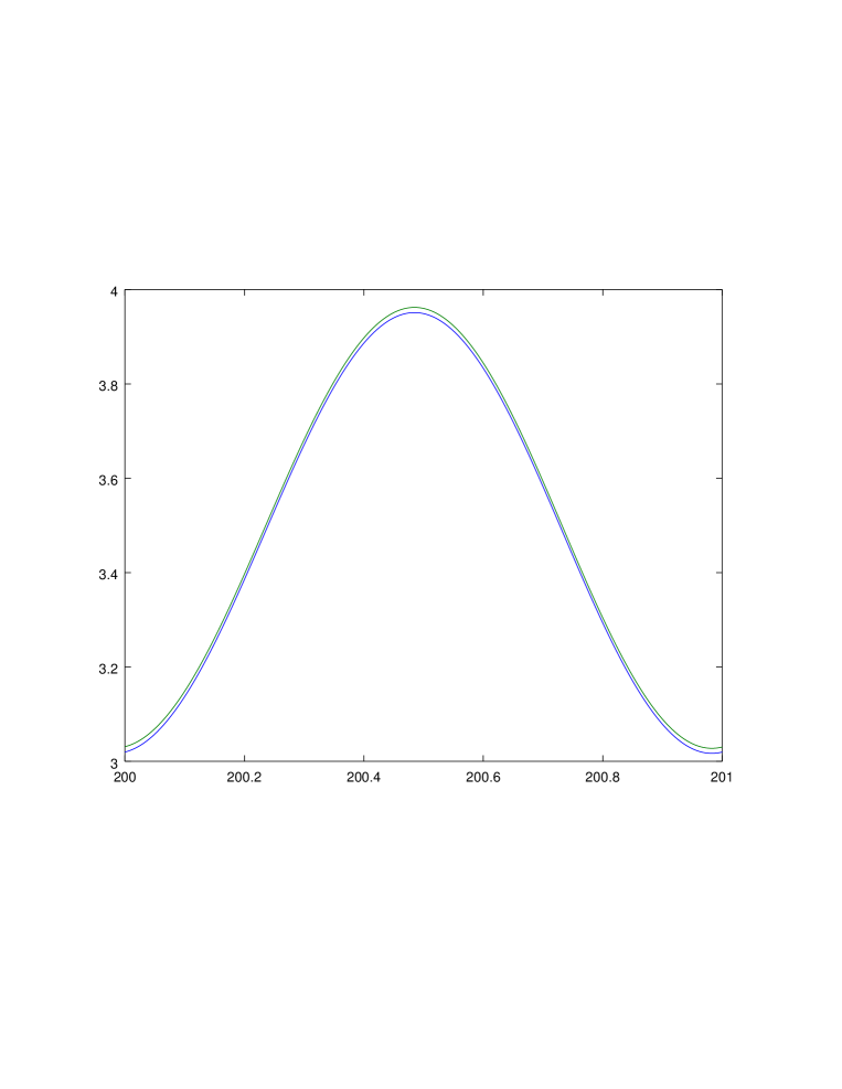
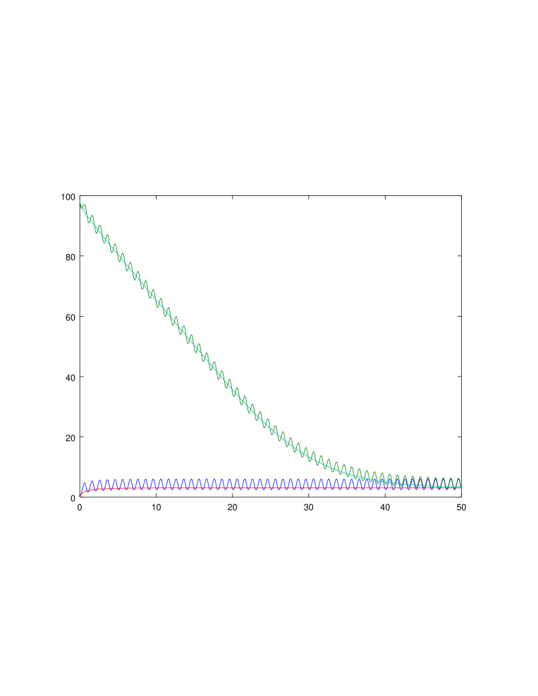
Figure 2: Example 1. Approximation of the mean for
with initial conditions and for
original and homogeneous situations.Figure 3: Example 1. Approximation of the mean for
with initial conditions and .Figure 4: Example 2. Approximation of the mean for
with initial conditions and for
original and homogeneous situations.Figure 5: Example 2. Approximation of the mean for
with initial conditions and .Figure 6: Example 3. Approximation of the mean for
with initial conditions and for
original and homogeneous situations.Figure 7: Example 3. Approximation of the mean for
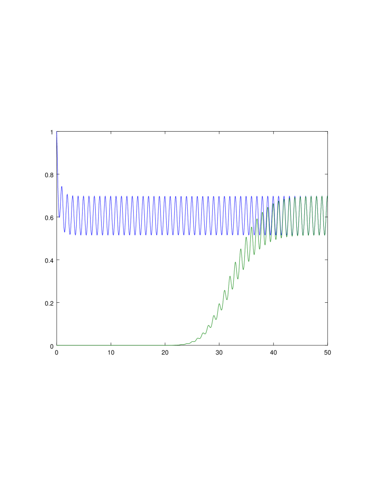
with initial conditions and .Figure 8: Example 1. Approximation of the probability for
with initial conditions and .Figure 9: Example 1. Approximation of the probability
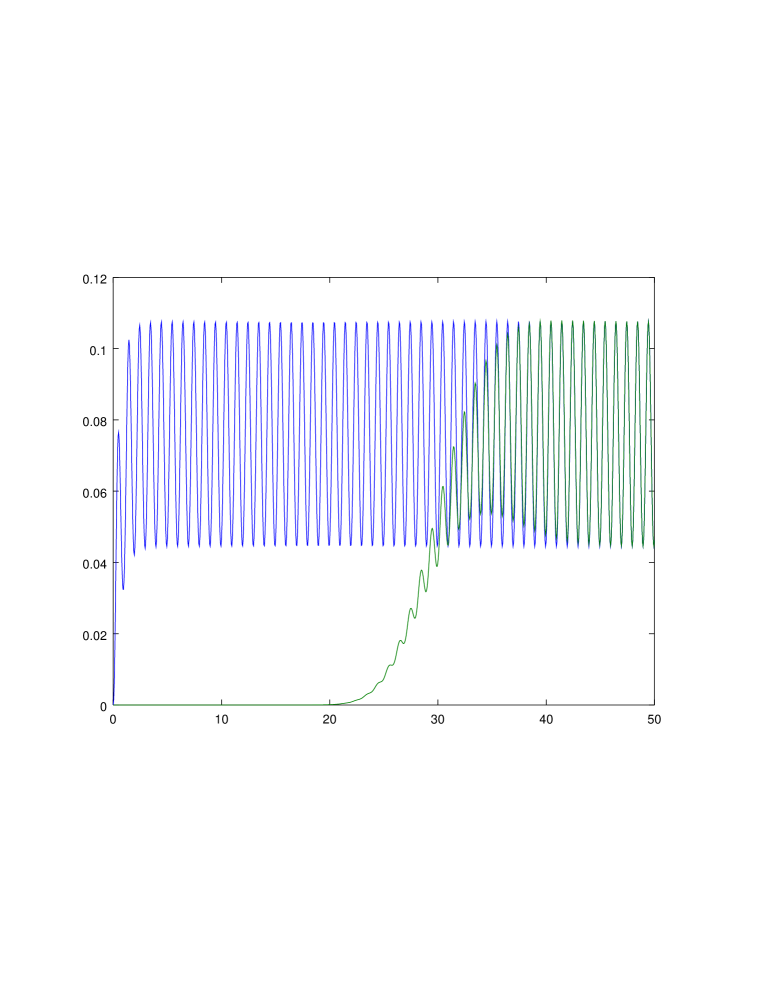
for with initial conditions and .Figure 10: Example 1. Approximation of the probability
for with initial conditions and .Figure 11: Example 1. Approximation of the probability
for with initial conditions and .Figure 12: Example 2. Approximation of the probability for
with initial conditions and .Figure 13: Example 2. Approximation of the probability
for with initial conditions and
.Figure 14: Example 2. Approximation of the probability
for with initial conditions and
.Figure 15: Example 2. Approximation of the probability
for with initial conditions and .Figure 16: Example 3. Approximation of the probability for
with initial conditions and .Figure 17: Example 3. Approximation of the probability
for with initial conditions and .Figure 18: Example 3. Approximation of the probability
for with initial conditions and .Figure 19: Example 3. Approximation of the probability
for with initial conditions and .