Integrable higher-dimensional cosmology with separable variables in an Einstein-dilaton-antisymmetric field theory

Abstract

We consider a $D$-dimensional cosmological model with a dilaton field and two $(D-d-1)$-form field strengths which have nonvanishing fluxes in extra dimensions. Exact solutions for the model with a certain set of couplings are obtained by separation of three variables. Some of the solutions describe accelerating expansion of the $d$-dimensional space. Quantum cosmological aspects of the model are also briefly mentioned.

I Introduction

In recent decades, relativistic models with a scalar field have received much interest in cosmology because they are suitable for the inflationary scenario inflation and for tackling the dark energy problems darkenergy1 ; darkenergy2 . Although numerical solutions or approximate solutions for scale factors are studied in many cosmological models, it would be very interesting to find exact solutions that describe the accelerating universe. In many areas of physics, exact solutions play the most important role in understanding and growing the crude concepts. Recently, many authors have studied integrable models with exponential scalar potentials for cosmology and found various interesting ones; for example, some models account for the transient acceleration of the universe STT ; Russo ; ENO ; FSS ; FST ; SS ; MP ; PM ; ANL ; ALNW .

On the other hand, it is known that dilaton gravity arises from a low-energy effective theory of string theory, from certain supergravity theories, and from higher-dimensional theories with extra dimensions. In models based on such theories, scalar fields naturally appear with exponential potentials. In addition, such theories often contain totally antisymmetric tensor fields; the configuration on the extra space can play an important role in compactification scheme MN1 ; MN2 ; GT ; Halliwell1 ; Halliwell2 . Some higher-dimensional integrable cosmological models have been studied Sano ; TW ; Ohta2 and exact analytic solutions have been derived in some specific cases with fluxes in extra dimensions LMPX ; Kaloper ; CGG ; Roy ; Ohta1 ; Ohta3 ; CHNOW ; Ohta4 .

In the present paper, we consider analytically solvable models of $D$-dimensional cosmology with a scalar dilaton and antisymmetric tensor fields. Integrability does not necessarily mean the existence of analytic solutions. We propose a model in which the equations of motion can be expressed by three separate equations of Liouville type; then, its cosmological solutions can be written in simple elementary functions. We analyze the simple model on the basis of the possibility of temporal accelerating expansion of the $(d+1)$-dimensional universe ($d+1<D$).

Here, we illustrate an essential structure of the solvable model we consider in this paper. Provided that the classical cosmological action (in the minisuperspace) can be written in the form

$$S=\int dt\sum_{a}\left[\sigma_{a}\frac{1}{2}\dot{x}_{a}^{2}-\frac{V_{a}}{2}e^{2\lambda_{a}x_{a}}\right]\,,$$ (1)

where $\sigma_{a}=\pm 1$ and the dot denotes the derivative with respect to $t$, the equations of motion give the one-dimensional Liouville equation

$$\sigma_{a}\ddot{x}_{a}+\lambda_{a}V_{a}e^{2\lambda_{a}x_{a}}=0\,.$$ (2)

Then, the integrals of motion are

$$E_{a}\equiv\sigma_{a}\frac{1}{2}\dot{x}_{a}^{2}+\frac{V_{a}}{2}e^{2\lambda_{a}x_{a}}\,.$$ (3)

We obtain the following analytic solutions for the equations of motion:

• For $\sigma_{a}V_{a}>0$,

  $$x_{a}(t)=\frac{1}{2\lambda_{a}}\ln\frac{q_{a}^{2}}{\cosh^{2}q_{a}\sqrt{|V_{a}|}\lambda_{a}(t-t_{a})}\,,\quad E_{a}=\sigma_{a}\frac{q_{a}^{2}|V_{a}|}{2}\,.$$ (4)

• For $\sigma_{a}V_{a}<0$,

  $$x_{a}(t)=\frac{1}{2\lambda_{a}}\ln\frac{q_{a}^{2}}{\sinh^{2}q_{a}\sqrt{|V_{a}|}\lambda_{a}(t-t_{a})}\,,\quad E_{a}=\sigma_{a}\frac{q_{a}^{2}|V_{a}|}{2}\,,$$ (5)

  $$x_{a}(t)=\frac{1}{2\lambda_{a}}\ln\frac{q_{a}^{2}}{\sin^{2}q_{a}\sqrt{|V_{a}|}\lambda_{a}(t-t_{a})}\,,\quad E_{a}=-\sigma_{a}\frac{q_{a}^{2}|V_{a}|}{2}\,.$$ (6)

• For $V_{a}=0$, we find that $x_{a}(t)=q_{a}(t-t_{a})$ and $E_{a}=\sigma_{a}\frac{q_{a}^{2}}{2}$,

where $q_{a}$ and $t_{a}$ are integration constants.

Remembering that the model is a cosmological one, the Hamiltonian constraint restricts the constants as

$$\sum_{a}\left[\sigma_{a}\frac{1}{2}\dot{x}_{a}^{2}+\frac{V_{a}}{2}e^{2\lambda_{a}x_{a}}\right]=\sum_{a}E_{a}=0\,.$$ (7)

We present a model that is soluble by using such a separation of variables in the next section. Furthermore, we will see later that the separation of variables is significant for considering the minisuperspace Wheeler–De Witt equation.

The outline of the present paper is as follows. In Sec. II, we define our models in which three variables are separable as in the manner mentioned above. The solutions are exhibited in Secs. III and IV, and summarized in Appendix A. Section III is devoted to the solutions for the scalar field with the canonical kinetic term, while Sec. IV treats the case of the “phantom” scalar field. The physical scale factor and the physical property of the solutions are discussed in Sec. V. Section VI contains a brief description of the quantum cosmology of our model through the minisuperspace Wheeler–De Witt equation. We conclude with a discussion in Sec. VII.

II action and variables

Let us consider the action of the $D$-dimensional model

$$S=\int d^{D}x\sqrt{-g}\left[R-\sigma\frac{1}{2}(\nabla\Phi)^{2}-\frac{l}{2p!}e^{2\kappa\alpha\Phi}{F_{[p]}^{(l)}}^{2}-\frac{r}{2p!}e^{-2\kappa\frac{\sigma}{\alpha}\Phi}{F_{[p]}^{(r)}}^{2}\right]\,,$$ (8)

where $R$ is the Ricci scalar derived from the metric $g_{MN}$ ($M,N=0,1,\dots,D-1$), $g$ is the determinant of $g_{MN}$, and $\Phi$ is a real scalar field which has dilatonlike coupling to the two $p$-form field strengths $F_{[p]}^{(l)}$ and $F_{[p]}^{(r)}$. The constant $\alpha$ represents a scalar (dilaton) self coupling constant. The constants $l$ and $r$ indicate the couplings between the scalar and the two antisymmetric tensor field strengths. We also use the abbreviations $(\nabla\Phi)^{2}\equiv g^{MN}\partial_{M}\Phi\partial_{N}\Phi$ and $F^{2}_{[p]}=g^{M_{1}N_{1}}g^{M_{2}N_{2}}\cdots g^{M_{p}N_{p}}{F_{[p]}}_{M_{1}M_{2}\cdots M_{p}}{F_{[p]}}_{N_{1}N_{2}\cdots N_{p}}$.

The action (8) is invariant under the following two independent transformations:

$$(1) \quad\alpha\leftrightarrow-\alpha\quad\mbox{and}\quad\Phi\leftrightarrow-\Phi\,,$$ (9)

$$(2) \quad\alpha\leftrightarrow-\sigma/\alpha\quad\mbox{and}\quad l\leftrightarrow r\quad\mbox{and}\quad F_{[p]}^{(l)}\leftrightarrow F_{[p]}^{(r)}\,.$$ (10)

If the constant $\sigma$ is taken to be $\sigma=+1$, the kinetic term of the scalar field becomes a canonical one. If we choose $\sigma=-1$, the scalar becomes a phantom field phantom . Due to the symmetries, we only have to investigate the cases with $0<\alpha\leq 1$ to clarify the general behaviors of the system. Note also that the choice $r=0$ in the action (8) reduces the model to that studied by many other authors, such as in Refs. CGG ; Roy . The value of the constant $\kappa$ will be specified later.

We adopt the following ansätze. We assume the $(D-1)$-dimensional space admits the metric of a direct product of a $d$-dimensional flat Euclidean space and $(D-d-1)$-dimensional maximally symmetric space. The scale factors and the scalar $\Phi$ are considered to be only time-dependent; i.e., they are functions of the time coordinate $t=x^{0}$. Therefore, we take the metric as follows:

$$ds^{2}=g_{MN}dx^{M}dx^{N}=-e^{2n(t)}dt^{2}+e^{2a(t)}d\mathbf{x}^{2}+e^{2b(t)}d\Omega_{D-d-1}^{2}\,.$$ (11)

Here, we denote the coordinates of the flat space as $x^{i}$ ($i=1,\dots,d$) and those of the maximal symmetric extra space as $x^{m}$ ($m=d+1,\dots,D-1$). We use the notation $d\mathbf{x}^{2}\equiv\sum_{i=1}^{d}(dx^{i})^{2}$, and $d\Omega_{[D-d-1]}^{2}$ stands for the line element of the extra space whose metric is denoted as $\tilde{g}_{mn}$. We assume that the Ricci tensor of the extra space is written as

$$\tilde{R}_{mn}=k_{b}(D-d-2)\tilde{g}_{mn}\,,$$ (12)

where $k_{b}$ is a constant, which has been normalized to $1$, $0$, or $-1$.

We further consistently assume that the $p$-form field strengths take “constant” (flux) values in the extra space; thus,

$$p=D-d-1\,$$ (13)

and

$${F_{[D-d-1]}^{(l)}}_{d+1,d+2,\cdots,{D-1}}={F_{[D-d-1]}^{(r)}}_{d+1,d+2,\cdots,{D-1}}=f\,,$$ (14)

where $f$ is taken as a positive constant (and is possibly quantized as a “magnetic” charge), without loss of generality. Even if we assume nonidentical values for two fluxes as classical configurations, the difference in the magnitudes of the fluxes can be absorbed into the redefinition of the couplings $l$ and $r$. We now obtain

$$\frac{1}{(D-d-1)!}({F_{[D-d-1]}^{(l)}})^{2}=\frac{1}{(D-d-1)!}({F_{[D-d-1]}^{(r)}})^{2}=f^{2}e^{-2(D-d-1)b}\,.$$ (15)

Substituting the anzätze and noting that $\sqrt{-g}\propto e^{da+(D-d-1)b+n}$, we find

$$S \propto \int dt\,\,e^{da+(D-d-1)b-n}$$ (16)

$$\quad\times\Bigl{\{}2d\ddot{a}+2(D-d-1)\ddot{b}+d(d+1)\dot{a}^{2}+2d(D-d-1)\dot{a}\dot{b}+(D-d)(D-d-1)\dot{b}^{2}$$

$$\qquad-2\dot{n}\left[d\dot{a}+(D-d-1)\dot{b}\right]+(D-d-1)(D-d-2)k_{b}e^{-2b+2n}+\sigma\frac{1}{2}\dot{\Phi}^{2}$$

$$\qquad-\frac{1}{2}f^{2}[le^{-2(D-d-1)b+2\kappa\alpha\Phi}+re^{-2(D-d-1)b-2\kappa\sigma\Phi/\alpha}]e^{2n}\Bigr{\}}\,,$$

where the dot indicates the derivative with respect to time $t$. Here, if we set

$$n(t)=da(t)+(D-d-1)b(t)\,$$ (17)

as a gauge choice, the reduced cosmological action becomes

$$S \propto \int dt\Bigl{\{}-d(d-1)\dot{a}^{2}-2d(D-d-1)\dot{a}\dot{b}-(D-d-1)(D-d-2)\dot{b}^{2}+\sigma\frac{1}{2}\dot{\Phi}^{2}$$ (18)

$$+(D-d-1)(D-d-2)k_{b}e^{2[da+(D-d-2)b]}-\frac{1}{2}f^{2}\left[le^{2[da+\kappa\alpha\Phi]}+re^{2[da-\kappa\sigma\Phi/\alpha]}\right]\Bigr{\}}\,.$$

We now find that the “kinetic” terms, which include the time derivatives, in the reduced action (18) can have a unique quadratic form as follows:

$$-d(d-1)\dot{a}^{2}-2d(D-d-1)\dot{a}\dot{b}-(D-d-1)(D-d-2)\dot{b}^{2}+\sigma\frac{1}{2}\dot{\Phi}^{2}$$ (19)

$$= -\frac{1}{2}\frac{2(D-d-1)}{D-d-2}\left[d\dot{a}+(D-d-2)\dot{b}\right]^{2}$$

$$+\frac{1}{2}\frac{\sigma}{\alpha^{2}+\sigma}\frac{2(D-2)}{d(D-d-2)}\left[d\dot{a}+\sqrt{\frac{d(D-d-2)}{2(D-2)}}\alpha\dot{\Phi}\right]^{2}$$

$$+\frac{1}{2}\frac{\alpha^{2}}{\alpha^{2}+\sigma}\frac{2(D-2)}{d(D-d-2)}\left[d\dot{a}-\sqrt{\frac{d(D-d-2)}{2(D-2)}}\frac{\sigma}{\alpha}\dot{\Phi}\right]^{2}\,.$$

Therefore, if we fix the constant

$$\kappa\equiv\sqrt{\frac{d(D-d-2)}{2(D-2)}}\,,$$ (20)

the action can be written in three independent variables $x\propto da+(D-d-2)b$, $y\propto da+\kappa\alpha\Phi$ and $z\propto da-\kappa\sigma\Phi/\alpha$.

We write the reduced action as $S=\int L\,dt$ with

$$L = -\frac{1}{2}\frac{2(D-d-1)}{D-d-2}\left[d\dot{a}+(D-d-2)\dot{b}\right]^{2}+\frac{1}{2}\frac{\sigma}{\alpha^{2}+\sigma}\frac{2(D-2)}{d(D-d-2)}\left[d\dot{a}+\kappa\alpha\dot{\Phi}\right]^{2}$$ (21)

$$+\frac{1}{2}\frac{\alpha^{2}}{\alpha^{2}+\sigma}\frac{2(D-2)}{d(D-d-2)}\left[d\dot{a}-\kappa\frac{\sigma}{\alpha}\dot{\Phi}\right]^{2}$$

$$-\frac{V_{1}}{2}e^{2[da+(D-d-2)b]}-\frac{1}{2}f^{2}\left[le^{2[da+\kappa\alpha\Phi]}+re^{2[da-\kappa\sigma\Phi/\alpha]}\right]\,,$$

where $V_{1}\equiv(D-d-1)(D-d-2)(-2k_{b})$.

Note that the coefficients of $[d\dot{a}+(D-d-2)\dot{b}]^{2}$ in the Lagrangian $L$ are independent of the dilaton coupling $\alpha$ and the kinematical signature $\sigma$. Therefore, we take a variable $x$ as

$$x(t)\equiv\sqrt{\frac{2(D-d-1)}{D-d-2}}\left[da+(D-d-2)b\right]\,,\\$$ (22)

throughout this paper. Then, the variable $x(t)$ obeys the equation

$$\ddot{x}+\lambda_{1}V_{1}e^{2\lambda_{1}x}=0\quad\mbox{with}\quad\lambda_{1}\equiv\sqrt{\frac{D-d-2}{2(D-d-1)}}\,.$$ (23)

The solution of Eq. (23) is

• (negative $E_{1}$)

  $$x(t)=\left\{\begin{array}[]{ll}x_{--1}(t)\equiv\frac{1}{2\lambda_{1}}\ln\frac{q_{1}^{2}}{\sinh^{2}q_{1}\sqrt{V_{1}}\lambda_{1}(t-t_{1})}&\mbox{for }k_{b}=-1\\ x_{-0}(t)\equiv q_{1}(t-t_{1})&\mbox{for }k_{b}=0\\ x_{-+1}(t)\equiv\frac{1}{2\lambda_{1}}\ln\frac{q_{1}^{2}}{\cosh^{2}q_{1}\sqrt{|V_{1}|}\lambda_{1}(t-t_{1})}&\mbox{for }k_{b}=+1\,,\end{array}\right.$$ (24)

  where $q_{1}$ and $t_{1}$ are constants.

  The first integral $E_{1}\equiv-\frac{1}{2}\dot{x}^{2}+\frac{V_{1}}{2}e^{2\lambda_{1}x}$ is

  $$E_{1}=\left\{\begin{array}[]{ll}E_{--1}\equiv-\frac{q_{1}^{2}V_{1}}{2}&\mbox{for }k_{b}=-1\\ E_{-0}\equiv-\frac{q_{1}^{2}}{2}&\mbox{for }k_{b}=0\\ E_{-+1}\equiv-\frac{q_{1}^{2}|V_{1}|}{2}&\mbox{for }k_{b}=+1\,,\end{array}\right.$$ (25)

  respectively.

• (positive $E_{1}$)

  $$x(t)=x_{+-1}(t)\equiv\frac{1}{2\lambda_{1}}\ln\frac{q_{1}^{2}}{\sin^{2}q_{1}\sqrt{V_{1}}\lambda_{1}(t-t_{1})}\quad\mbox{for}\quad k_{b}=-1\,,$$ (26)

  where $q_{1}$ and $t_{1}$ are constants.

  The first integral $E_{1}=-\frac{1}{2}\dot{x}^{2}+\frac{V_{1}}{2}e^{2\lambda_{1}x}$ is

  $$E_{1}=E_{+-1}\equiv\frac{q_{1}^{2}V_{1}}{2}\quad\mbox{for}\quad k_{b}=-1\,.$$ (27)

In the next section, we study the model with $\sigma=+1$ and derive exact solutions. The case with $\sigma=-1$ is treated in Sec. IV.

III case for the canonical kinetic term of the dilaton ($\sigma=1$)

For $\sigma=+1$, the reduced cosmological Lagrangian is written as

$$L=-\frac{1}{2}\dot{x}^{2}+\frac{1}{2}\dot{y}^{2}+\frac{1}{2}\dot{z}^{2}-\frac{V_{1}}{2}e^{2\lambda_{1}x}-\frac{lf^{2}}{2}e^{2\lambda_{2}y}-\frac{rf^{2}}{2}e^{2\lambda_{3}z}\,,$$ (28)

where

$$\lambda_{2}y\equiv da+\kappa\alpha\Phi\,,\,\lambda_{3}z\equiv da-\frac{\kappa}{\alpha}\Phi\quad\mbox{with}\quad\lambda_{2}\equiv\sqrt{\alpha^{2}+1}\,\kappa\,,\,\lambda_{3}\equiv\sqrt{{\alpha^{-2}+1}}\,\kappa\,.$$ (29)

We permit arbitrary signs of $l$ and $r$ in the present paper. When a negative sign of the coefficient is taken, it yields a “phantom” gauge field. Such a phantom gauge field has been considered in a cosmological context KS , though their negative value may lead to pathological consequences in quantum physics.

The exact solution of the model can now be obtained in each case shown below. In this section, we define integrals of motion as

$$E_{2}\equiv\frac{1}{2}\dot{y}^{2}+\frac{lf^{2}}{2}e^{2\lambda_{2}y}\,,\quad E_{3}\equiv\frac{1}{2}\dot{z}^{2}+\frac{rf^{2}}{2}e^{2\lambda_{3}z}\,.$$ (30)

III.1 Case $l>0$ and $r>0$

First, in this case, we find that the solutions for $y$ and $z$ for the reduced Lagrangian $L$ can be written as

$$y(t)=\frac{1}{2\lambda_{2}}\ln\frac{q_{2}^{2}}{\cosh^{2}q_{2}\sqrt{l}f\lambda_{2}(t-t_{2})}\,,\quad z(t)=\frac{1}{2\lambda_{3}}\ln\frac{q_{3}^{2}}{\cosh^{2}q_{3}\sqrt{r}f\lambda_{3}(t-t_{3})}\,,$$ (31)

where $q_{2}$, $t_{2}$, $q_{3}$, and $t_{3}$ are integration constants. Then, both $E_{2}$ and $E_{3}$ are positive. Since the Hamiltonian constraint gives $E_{1}+E_{2}+E_{3}=0$, a possible solution of $x(t)$ is $x_{-k_{b}}(t)$ defined in Sec. II. The Hamiltonian constraint then reads

$$lf^{2}q_{2}^{2}+rf^{2}q_{3}^{2}=|V_{1}|q_{1}^{2}\quad\mbox{for }k_{b}=\pm 1\,,\quad lf^{2}q_{2}^{2}+rf^{2}q_{3}^{2}=q_{1}^{2}\quad\mbox{for }k_{b}=0\,.$$ (32)

III.2 Case $l>0$ and $r<0$

In this case, the exact solution for $y$ is written as

$$y(t)=\frac{1}{2\lambda_{2}}\ln\frac{q_{2}^{2}}{\cosh^{2}q_{2}\sqrt{l}f\lambda_{2}(t-t_{2})}\,,$$ (33)

where $q_{2}$ and $t_{2}$ are constants, and then $E_{2}>0$. The solutions of other variables are characterized by the following subcategories, according to the signature of $E_{1}$ and $E_{3}$.

III.2.1 $E_{1}<0$ and $E_{3}>0$

The solution for $x$ is $x_{-k_{b}}(t)$, and the solution for $z$ is

$$z(t)=\frac{1}{2\lambda_{3}}\ln\frac{q_{3}^{2}}{\sinh^{2}q_{3}\sqrt{|r|}f\lambda_{3}(t-t_{3})}\,,$$ (34)

where $q_{3}$ and $t_{3}$ are constants. Then, the Hamiltonian constraint becomes

$$lf^{2}q_{2}^{2}+|r|f^{2}q_{3}^{2}-|V_{1}|q_{1}^{2}=0\quad\mbox{for}\quad k_{b}=\pm 1\,,\quad lf^{2}q_{2}^{2}+|r|f^{2}q_{3}^{2}-q_{1}^{2}=0\quad\mbox{for}\quad k_{b}=0\,.$$ (35)

III.2.2 $E_{1}<0$ and $E_{3}<0$

The solution for $x$ is $x_{-k_{b}}(t)$, and the solution for $z$ is

$$z(t)=\frac{1}{2\lambda_{3}}\ln\frac{q_{3}^{2}}{\sin^{2}q_{3}\sqrt{|r|}f\lambda_{3}(t-t_{3})}\,,$$ (36)

where $q_{3}$ and $t_{3}$ are constants. Then, the Hamiltonian constraint becomes

$$lf^{2}q_{2}^{2}-|r|f^{2}q_{3}^{2}-|V_{1}|q_{1}^{2}=0\quad\mbox{for}\quad k_{b}=\pm 1\,,\quad lf^{2}q_{2}^{2}-|r|f^{2}q_{3}^{2}-q_{1}^{2}=0\quad\mbox{for}\quad k_{b}=0\,.$$ (37)

III.2.3 $E_{1}>0$ and $E_{3}<0$

The solution for $x$ is $x_{+-1}(t)$, and the solution for $z$ is

$$z(t)=\frac{1}{2\lambda_{3}}\ln\frac{q_{3}^{2}}{\sin^{2}q_{3}\sqrt{|r|}f\lambda_{3}(t-t_{3})}\,,$$ (38)

where $q_{3}$ and $t_{3}$ are constants. Then, the Hamiltonian constraint becomes

$$lf^{2}q_{2}^{2}-|r|f^{2}q_{3}^{2}+V_{1}q_{1}^{2}=0\quad\mbox{for}\quad k_{b}=-1\,.$$ (39)

III.3 Case $l<0$ and $r>0$

This case can be regarded as the previous case where the roles of $y$ and $z$ are mutually exchanged. The exact solution for $z$ is written as

$$z(t)=\frac{1}{2\lambda_{3}}\ln\frac{q_{3}^{2}}{\cosh^{2}q_{3}\sqrt{r}f\lambda_{3}(t-t_{3})}\,,$$ (40)

where $q_{3}$ and $t_{3}$ are constants, and then $E_{3}>0$. Solutions of other variables are characterized by the following subcategories, according to the signature of $E_{1}$ and $E_{2}$.

III.3.1 $E_{1}<0$ and $E_{2}>0$

The solution for $x$ is $x_{-k_{b}}(t)$, and the solution for $y$ is

$$y(t)=\frac{1}{2\lambda_{2}}\ln\frac{q_{2}^{2}}{\sinh^{2}q_{2}\sqrt{|l|}f\lambda_{2}(t-t_{2})}\,,$$ (41)

where $q_{2}$ and $t_{2}$ are constants. Then, the Hamiltonian constraint becomes

$$|l|f^{2}q_{2}^{2}+rf^{2}q_{3}^{2}-|V_{1}|q_{1}^{2}=0\quad\mbox{for}\quad k_{b}=\pm 1\,,\quad|l|f^{2}q_{2}^{2}+rf^{2}q_{3}^{2}-q_{1}^{2}=0\quad\mbox{for}\quad k_{b}=0\,.$$ (42)

III.3.2 $E_{1}<0$ and $E_{2}<0$

The solution for $x$ is $x_{-k_{b}}(t)$, and the solution for $y$ is

$$y(t)=\frac{1}{2\lambda_{2}}\ln\frac{q_{2}^{2}}{\sin^{2}q_{2}\sqrt{|l|}f\lambda_{2}(t-t_{2})}\,,$$ (43)

where $q_{2}$ and $t_{2}$ are constants. Then, the Hamiltonian constraint becomes

$$-|l|f^{2}q_{2}^{2}+rf^{2}q_{3}^{2}-|V_{1}|q_{1}^{2}=0\quad\mbox{for}\quad k_{b}=\pm 1\,,\quad-|l|f^{2}q_{2}^{2}+rf^{2}q_{3}^{2}-q_{1}^{2}=0\quad\mbox{for}\quad k_{b}=0\,.$$ (44)

III.3.3 $E_{1}>0$ and $E_{2}<0$

The solution for $x$ is $x_{+-1}(t)$, and the solution for $y$ is

$$y(t)=\frac{1}{2\lambda_{2}}\ln\frac{q_{2}^{2}}{\sin^{2}q_{2}\sqrt{|l|}f\lambda_{2}(t-t_{2})}\,,$$ (45)

where $q_{2}$ and $t_{2}$ are constants. Then, the Hamiltonian constraint becomes

$$-|l|f^{2}q_{2}^{2}+rf^{2}q_{3}^{2}+V_{1}q_{1}^{2}=0\quad\mbox{for}\quad k_{b}=-1\,.$$ (46)

III.4 Case $l<0$ and $r<0$

In this case, various forms of the exact solutions appear since each integral of motion can take a positive or negative value.

III.4.1 $E_{1}<0$, $E_{2}>0$, and $E_{3}>0$

The solution for $x$ is $x_{-k_{b}}(t)$, and the solutions for $y$ and $z$ are

$$y(t)=\frac{1}{2\lambda_{2}}\ln\frac{q_{2}^{2}}{\sinh^{2}q_{2}\sqrt{|l|}f\lambda_{2}(t-t_{2})}\,,\quad z(t)=\frac{1}{2\lambda_{3}}\ln\frac{q_{3}^{2}}{\sinh^{2}q_{3}\sqrt{|r|}f\lambda_{3}(t-t_{3})}\,,$$ (47)

where $q_{2}$, $t_{2}$, $q_{3}$, and $t_{3}$ are constants. Then, the Hamiltonian constraint becomes

$$|l|f^{2}q_{2}^{2}+|r|f^{2}q_{3}^{2}-|V_{1}|q_{1}^{2}=0\quad\mbox{for}\quad k_{b}=\pm 1\,,\quad|l|f^{2}q_{2}^{2}+|r|f^{2}q_{3}^{2}-q_{1}^{2}=0\quad\mbox{for}\quad k_{b}=0\,.$$ (48)

III.4.2 $E_{1}<0$, $E_{2}>0$, and $E_{3}<0$

The solution for $x$ is $x_{-k_{b}}(t)$, and the solutions for $y$ and $z$ are

$$y(t)=\frac{1}{2\lambda_{2}}\ln\frac{q_{2}^{2}}{\sinh^{2}q_{2}\sqrt{|l|}f\lambda_{2}(t-t_{2})}\,,\quad z(t)=\frac{1}{2\lambda_{3}}\ln\frac{q_{3}^{2}}{\sin^{2}q_{3}\sqrt{|r|}f\lambda_{3}(t-t_{3})}\,,$$ (49)

where $q_{2}$, $t_{2}$, $q_{3}$, and $t_{3}$ are constants. Then, the Hamiltonian constraint becomes

$$|l|f^{2}q_{2}^{2}-|r|f^{2}q_{3}^{2}-|V_{1}|q_{1}^{2}=0\quad\mbox{for}\quad k_{b}=\pm 1\,,\quad|l|f^{2}q_{2}^{2}-|r|f^{2}q_{3}^{2}-q_{1}^{2}=0\quad\mbox{for}\quad k_{b}=0\,.$$ (50)

III.4.3 $E_{1}<0$, $E_{2}<0$, and $E_{3}>0$

The solution for $x$ is $x_{-k_{b}}(t)$, and the solutions for $y$ and $z$ are

$$y(t)=\frac{1}{2\lambda_{2}}\ln\frac{q_{2}^{2}}{\sin^{2}q_{2}\sqrt{|l|}f\lambda_{2}(t-t_{2})}\,,\quad z(t)=\frac{1}{2\lambda_{3}}\ln\frac{q_{3}^{2}}{\sinh^{2}q_{3}\sqrt{|r|}f\lambda_{3}(t-t_{3})}\,,$$ (51)

where $q_{2}$, $t_{2}$, $q_{3}$, and $t_{3}$ are constants. Then, the Hamiltonian constraint becomes

$$-|l|f^{2}q_{2}^{2}+|r|f^{2}q_{3}^{2}-|V_{1}|q_{1}^{2}=0\quad\mbox{for}\quad k_{b}=\pm 1\,,\quad-|l|f^{2}q_{2}^{2}+|r|f^{2}q_{3}^{2}-q_{1}^{2}=0\quad\mbox{for}\quad k_{b}=0\,.$$ (52)

III.4.4 $E_{1}>0$, $E_{2}<0$, and $E_{3}<0$

The solution for $x$ is $x_{+-1}(t)$, and the solutions for $y$ and $z$ are

$$y(t)=\frac{1}{2\lambda_{2}}\ln\frac{q_{2}^{2}}{\sin^{2}q_{2}\sqrt{|l|}f\lambda_{2}(t-t_{2})}\,,\quad z(t)=\frac{1}{2\lambda_{3}}\ln\frac{q_{3}^{2}}{\sin^{2}q_{3}\sqrt{|r|}f\lambda_{3}(t-t_{3})}\,,$$ (53)

where $q_{2}$, $t_{2}$, $q_{3}$, and $t_{3}$ are constants. Then, the Hamiltonian constraint becomes

$$-|l|f^{2}q_{2}^{2}-|r|f^{2}q_{3}^{2}+V_{1}q_{1}^{2}=0\quad\mbox{for}\quad k_{b}=-1\,.$$ (54)

III.4.5 $E_{1}>0$, $E_{2}>0$, and $E_{3}<0$

The solution for $x$ is $x_{+-1}(t)$, and the solutions for $y$ and $z$ are

$$y(t)=\frac{1}{2\lambda_{2}}\ln\frac{q_{2}^{2}}{\sinh^{2}q_{2}\sqrt{|l|}f\lambda_{2}(t-t_{2})}\,,\quad z(t)=\frac{1}{2\lambda_{3}}\ln\frac{q_{3}^{2}}{\sin^{2}q_{3}\sqrt{|r|}f\lambda_{3}(t-t_{3})}\,,$$ (55)

where $q_{2}$, $t_{2}$, $q_{3}$, and $t_{3}$ are constants. Then, the Hamiltonian constraint becomes

$$|l|f^{2}q_{2}^{2}-|r|f^{2}q_{3}^{2}+V_{1}q_{1}^{2}=0\quad\mbox{for}\quad k_{b}=-1\,,$$ (56)

III.4.6 $E_{1}>0$, $E_{2}<0$, and $E_{3}>0$

The solution for $x$ is $x_{+-1}(t)$, and the solutions for $y$ and $z$ are

$$y(t)=\frac{1}{2\lambda_{2}}\ln\frac{q_{2}^{2}}{\sin^{2}q_{2}\sqrt{|l|}f\lambda_{2}(t-t_{2})}\,,\quad z(t)=\frac{1}{2\lambda_{3}}\ln\frac{q_{3}^{2}}{\sinh^{2}q_{3}\sqrt{|r|}f\lambda_{3}(t-t_{3})}\,,$$ (57)

where $q_{2}$, $t_{2}$, $q_{3}$, and $t_{3}$ are constants. Then, the Hamiltonian constraint becomes

$$-|l|f^{2}q_{2}^{2}+|r|f^{2}q_{3}^{2}+V_{1}q_{1}^{2}=0\quad\mbox{for}\quad k_{b}=-1\,.$$ (58)

Now, all the solutions for $x$, $y$, and $z$ have been shown for $\sigma=+1$. In the next section, we examine the case with $\sigma=-1$, which corresponds to a phantom dilaton.

IV The case for a phantom dilaton ($\sigma=-1$)

In this section, we consider the case with $\sigma=-1$. Remembering $0<\alpha<1$, the reduced action can be written as

$$L=-\frac{1}{2}\dot{x}^{2}+\frac{1}{2}\dot{y}^{2}-\frac{1}{2}\dot{z}^{2}-\frac{V_{1}}{2}e^{2\lambda_{1}x}-\frac{lf^{2}}{2}e^{2\lambda_{2}y}-\frac{rf^{2}}{2}e^{2\lambda_{3}z}\,,$$ (59)

where

$$\lambda_{2}y\equiv da+\kappa\alpha\Phi\,,\,\lambda_{3}z\equiv da+\frac{\kappa}{\alpha}\Phi\quad\mbox{with}\quad\lambda_{2}=\sqrt{1-\alpha^{2}}\,\kappa\,,\,\lambda_{3}=\sqrt{\alpha^{-2}-1}\,\kappa\,.$$ (60)

Similarly to the previous section, we obtain exact solutions for the cases with positive and negative couplings $l$ and $r$. In this section, we define

$$E_{2}\equiv\frac{1}{2}\dot{y}^{2}+\frac{lf^{2}}{2}e^{2\lambda_{2}y}\,,\quad E_{3}\equiv-\frac{1}{2}\dot{z}^{2}+\frac{rf^{2}}{2}e^{2\lambda_{3}z}\,.$$ (61)

IV.1 Case $l>0$ and $r>0$

In this case, the solution for $y$ takes the form

$$y(t)=\frac{1}{2\lambda_{2}}\ln\frac{q_{2}^{2}}{\cosh^{2}q_{2}\sqrt{l}f\lambda_{2}(t-t_{2})}\,,$$ (62)

where $q_{2}$ and $t_{2}$ are constants, and then $E_{2}>0$. Similarly to the previous section, several cases are classified below.

IV.1.1 $E_{1}<0$ and $E_{3}>0$

The solution for $x$ is $x_{-k_{b}}(t)$, and the solution for $z$ is given by

$$z(t)=\frac{1}{2\lambda_{3}}\ln\frac{q_{3}^{2}}{\sin^{2}q_{3}\sqrt{r}f\lambda_{3}(t-t_{3})}\,,$$ (63)

where $q_{3}$ and $t_{3}$ are constants. The Hamiltonian constraint becomes

$$lf^{2}q_{2}^{2}+rf^{2}q_{3}^{2}-|V_{1}|q_{1}^{2}=0\quad\mbox{for}\quad k_{b}=\pm 1\,,\quad lf^{2}q_{2}^{2}+rf^{2}q_{3}^{2}-q_{1}^{2}=0\quad\mbox{for}\quad k_{b}=0\,.$$ (64)

IV.1.2 $E_{1}<0$ and $E_{3}<0$

The solution for $x$ is $x_{-k_{b}}(t)$, and the solutions for $z$ is

$$z(t)=\frac{1}{2\lambda_{3}}\ln\frac{q_{3}^{2}}{\sinh^{2}q_{3}\sqrt{r}f\lambda_{3}(t-t_{3})}\,,$$ (65)

where $q_{3}$ and $t_{3}$ are constants. The Hamiltonian constraint becomes

$$lf^{2}q_{2}^{2}-rf^{2}q_{3}^{2}-|V_{1}|q_{1}^{2}=0\quad\mbox{for}\quad k_{b}=\pm 1\,,\quad lf^{2}q_{2}^{2}-rf^{2}q_{3}^{2}-q_{1}^{2}=0\quad\mbox{for}\quad k_{b}=0\,.$$ (66)

IV.1.3 $E_{1}>0$ and $E_{3}<0$

The solution for $x$ is $x_{+-1}(t)$, and the solution for $z$ is

$$z(t)=\frac{1}{2\lambda_{3}}\ln\frac{q_{3}^{2}}{\sinh^{2}q_{3}\sqrt{r}f\lambda_{3}(t-t_{3})}\,,$$ (67)

where $q_{3}$ and $t_{3}$ are constants. The Hamiltonian constraint becomes

$$lf^{2}q_{2}^{2}-rf^{2}q_{3}^{2}+V_{1}q_{1}^{2}=0\quad\mbox{for}\quad k_{b}=-1\,.$$ (68)

IV.2 Case $l>0$ and $r<0$

In this case, the solutions for $y$ and $z$ are given by

$$y(t)=\frac{1}{2\lambda_{2}}\ln\frac{q_{2}^{2}}{\cosh^{2}q_{2}\sqrt{l}f\lambda_{2}(t-t_{2})}\,,\quad z(t)=\frac{1}{2\lambda_{3}}\ln\frac{q_{3}^{2}}{\cosh^{2}q_{3}\sqrt{r}f\lambda_{3}(t-t_{3})}\,,$$ (69)

where $q_{2}$, $t_{2}$, $q_{3}$, and $t_{3}$ are constants, and then $E_{2}>$ and $E_{3}<0$.

IV.2.1 $E_{1}<0$

The solution for $x$ is $x_{-k_{b}}(t)$. The Hamiltonian constraint reads

$$lf^{2}q_{2}^{2}-|r|f^{2}q_{3}^{2}-|V_{1}|q_{1}^{2}=0\quad\mbox{for}\quad k_{b}=\pm 1\,,\quad lf^{2}q_{2}^{2}-|r|f^{2}q_{3}^{2}-q_{1}^{2}=0\quad\mbox{for}\quad k_{b}=0\,.$$ (70)

IV.2.2 $E_{1}>0$

The solution for $x$ is $x_{+-1}(t)$. The Hamiltonian constraint reads

$$lf^{2}q_{2}^{2}-|r|f^{2}q_{3}^{2}+V_{1}q_{1}^{2}=0\quad\mbox{for}\quad k_{b}=-1\,.$$ (71)

IV.3 Case $l<0$ and $r>0$

In this case, all possible signs for $E_{1}$, $E_{2}$, and $E_{3}$ can appear.

IV.3.1 $E_{1}<0$, $E_{2}>0$, and $E_{3}>0$

The solution for $x$ is $x_{-k_{b}}(t)$. The solutions for $y$ and $z$ are

$$y(t)=\frac{1}{2\lambda_{2}}\ln\frac{q_{2}^{2}}{\sinh^{2}q_{2}\sqrt{|l|}f\lambda_{2}(t-t_{2})}\,,\quad z(t)=\frac{1}{2\lambda_{3}}\ln\frac{q_{3}^{2}}{\sin^{2}q_{3}\sqrt{r}f\lambda_{3}(t-t_{3})}\,.$$ (72)

The Hamiltonian constraint is

$$|l|f^{2}q_{2}^{2}+rf^{2}q_{3}^{2}-|V_{1}|q_{1}^{2}=0\quad\mbox{for}\quad k_{b}=\pm 1\,,\quad|l|f^{2}q_{2}^{2}+rf^{2}q_{3}^{2}-q_{1}^{2}=0\quad\mbox{for}\quad k_{b}=0\,.$$ (73)

IV.3.2 $E_{1}<0$, $E_{2}>0$, and $E_{3}<0$

The solution for $x$ is $x_{-k_{b}}(t)$. The solutions for $y$ and $z$ are

$$y(t)=\frac{1}{2\lambda_{2}}\ln\frac{q_{2}^{2}}{\sinh^{2}q_{2}\sqrt{|l|}f\lambda_{2}(t-t_{2})}\,,\quad z(t)=\frac{1}{2\lambda_{3}}\ln\frac{q_{3}^{2}}{\sinh^{2}q_{3}\sqrt{r}f\lambda_{3}(t-t_{3})}\,.$$ (74)

The Hamiltonian constraint is

$$|l|f^{2}q_{2}^{2}-rf^{2}q_{3}^{2}-|V_{1}|q_{1}^{2}=0\quad\mbox{for}\quad k_{b}=\pm 1\,,\quad|l|f^{2}q_{2}^{2}-rf^{2}q_{3}^{2}-q_{1}^{2}=0\quad\mbox{for}\quad k_{b}=0\,.$$ (75)

IV.3.3 $E_{1}<0$, $E_{2}<0$, and $E_{3}>0$

The solution for $x$ is $x_{-k_{b}}(t)$. The solutions for $y$ and $z$ are

$$y(t)=\frac{1}{2\lambda_{2}}\ln\frac{q_{2}^{2}}{\sin^{2}q_{2}\sqrt{|l|}f\lambda_{2}(t-t_{2})}\,,\quad z(t)=\frac{1}{2\lambda_{3}}\ln\frac{q_{3}^{2}}{\sin^{2}q_{3}\sqrt{r}f\lambda_{3}(t-t_{3})}\,.$$ (76)

The Hamiltonian constraint is

$$-|l|f^{2}q_{2}^{2}+rf^{2}q_{3}^{2}-|V_{1}|q_{1}^{2}=0\quad\mbox{for}\quad k_{b}=\pm 1\,,\quad-|l|f^{2}q_{2}^{2}+rf^{2}q_{3}^{2}-q_{1}^{2}=0\quad\mbox{for}\quad k_{b}=0\,.$$ (77)

IV.3.4 $E_{1}>0$, $E_{2}>0$, and $E_{3}<0$

The solution for $x$ is $x_{+-1}(t)$. The solutions for $y$ and $z$ are

$$y(t)=\frac{1}{2\lambda_{2}}\ln\frac{q_{2}^{2}}{\sinh^{2}q_{2}\sqrt{|l|}f\lambda_{2}(t-t_{2})}\,,\quad z(t)=\frac{1}{2\lambda_{3}}\ln\frac{q_{3}^{2}}{\sinh^{2}q_{3}\sqrt{r}f\lambda_{3}(t-t_{3})}\,.$$ (78)

The Hamiltonian constraint is

$$|l|f^{2}q_{2}^{2}-rf^{2}q_{3}^{2}+V_{1}q_{1}^{2}=0\quad\mbox{for}\quad k_{b}=-1\,.$$ (79)

IV.3.5 $E_{1}>0$, $E_{2}<0$, and $E_{3}>0$

The solution for $x$ is $x_{+-1}(t)$. The solutions for $y$ and $z$ are

$$y(t)=\frac{1}{2\lambda_{2}}\ln\frac{q_{2}^{2}}{\sin^{2}q_{2}\sqrt{|l|}f\lambda_{2}(t-t_{2})}\,,\quad z(t)=\frac{1}{2\lambda_{3}}\ln\frac{q_{3}^{2}}{\sin^{2}q_{3}\sqrt{r}f\lambda_{3}(t-t_{3})}\,.$$ (80)

The Hamiltonian constraint is

$$-|l|f^{2}q_{2}^{2}+rf^{2}q_{3}^{2}+V_{1}q_{1}^{2}=0\quad\mbox{for}\quad k_{b}=-1\,.$$ (81)

IV.3.6 $E_{1}>0$, $E_{2}<0$, and $E_{3}<0$

The solution for $x$ is $x_{+-1}(t)$. The solutions for $y$ and $z$ are

$$y(t)=\frac{1}{2\lambda_{2}}\ln\frac{q_{2}^{2}}{\sin^{2}q_{2}\sqrt{|l|}f\lambda_{2}(t-t_{2})}\,,\quad z(t)=\frac{1}{2\lambda_{3}}\ln\frac{q_{3}^{2}}{\sinh^{2}q_{3}\sqrt{r}f\lambda_{3}(t-t_{3})}\,.$$ (82)

The Hamiltonian constraint is

$$-|l|f^{2}q_{2}^{2}-rf^{2}q_{3}^{2}+V_{1}q_{1}^{2}=0\quad\mbox{for}\quad k_{b}=-1\,.$$ (83)

IV.4 Case $l<0$ and $r<0$

In this case, the solution for $z$ is

$$z(t)=\frac{1}{2\lambda_{3}}\ln\frac{q_{3}^{2}}{\cosh^{2}q_{3}\sqrt{|r|}f\lambda_{3}(t-t_{3})}\,,$$ (84)

and then $E_{3}<0$.

IV.4.1 $E_{1}<0$ and $E_{2}>0$

The solution for $x$ is $x_{-k_{b}}(t)$, and the solution for $y$ is

$$y(t)=\frac{1}{2\lambda_{2}}\ln\frac{q_{2}^{2}}{\sinh^{2}q_{2}\sqrt{|l|}f\lambda_{2}(t-t_{2})}\,,$$ (85)

where $q_{2}$ and $t_{2}$ are constants. The Hamiltonian constraint reads

$$|l|f^{2}q_{2}^{2}-|r|f^{2}q_{3}^{2}-|V_{1}|q_{1}^{2}=0\quad\mbox{for}\quad k_{b}=\pm 1\,,\quad|l|f^{2}q_{2}^{2}-|r|f^{2}q_{3}^{2}-q_{1}^{2}=0\quad\mbox{for}\quad k_{b}=0\,.$$ (86)

IV.4.2 $E_{1}>0$ and $E_{2}>0$

The solution for $x$ is $x_{+-1}(t)$, and the solution for $y$ is

$$y(t)=\frac{1}{2\lambda_{2}}\ln\frac{q_{2}^{2}}{\sinh^{2}q_{2}\sqrt{|l|}f\lambda_{2}(t-t_{2})}\,,$$ (87)

where $q_{2}$ and $t_{2}$ are constants. The Hamiltonian constraint reads

$$|l|f^{2}q_{2}^{2}-|r|f^{2}q_{3}^{2}+V_{1}q_{1}^{2}=0\quad\mbox{for}\quad k_{b}=-1\,.$$ (88)

IV.4.3 $E_{1}>0$ and $E_{2}<0$

The solution for $x$ is $x_{+-1}(t)$, and the solution for $y$ is

$$y(t)=\frac{1}{2\lambda_{2}}\ln\frac{q_{2}^{2}}{\sin^{2}q_{2}\sqrt{|l|}f\lambda_{2}(t-t_{2})}\,,$$ (89)

where $q_{2}$ and $t_{2}$ are constants. The Hamiltonian constraint reads

$$-|l|f^{2}q_{2}^{2}-|r|f^{2}q_{3}^{2}+V_{1}q_{1}^{2}=0\quad\mbox{for}\quad k_{b}=-1\,.$$ (90)

V Accelerating universe

To analyze the cosmological behavior closely, we introduce the “physical ” $(d+1)$-dimensional metric and the cosmic time. When we take a representation for the $D$-dimensional metric such as

$$ds^{2} = e^{-\frac{2(D-d-1)b}{d-1}}\bar{g}_{\mu\nu}dx^{\mu}dx^{\nu}+e^{2b}\tilde{g}_{mn}dx^{m}dx^{n}\,,$$ (91)

we find that $\sqrt{-g}R$ is proportional to $\sqrt{-\bar{g}}\bar{R}+\cdots$, where $\bar{R}$ is the Ricci scalar of the $(d+1)$-dimensional spacetime constructed from $\bar{g}_{\mu\nu}$. Therefore, the metric $\bar{g}_{\mu\nu}$ is considered to define the Einstein frame of the $(d+1)$-dimensional spacetime.

In the present study, we should regard the following form for the metric:

$$ds^{2} = -e^{2[da(t)+(D-d-1)b(t)]}dt^{2}+e^{2a(t)}d\mathbf{x}^{2}+e^{2b(t)}d\Omega_{D-d-1}^{2}$$ (92)

$$= e^{-\frac{2(D-d-1)b}{d-1}}(-d\eta^{2}+S^{2}(\eta)d\mathbf{x}^{2})+e^{2b}d\Omega_{D-d-1}^{2}\,,$$

where $\eta$ is the cosmic time for the $(d+1)$-dimensional spacetime and $S$ is the “physical” scale factor of $d$-dimensional flat space in the $(d+1)$-dimensional view. Thus, we obtain the relations

$$S(\eta)=e^{a(t)+\frac{D-d-1}{d-1}b(t)}\,,\quad d\eta=\pm e^{d[a(t)+\frac{D-d-1}{d-1}b(t)]}dt=\pm S^{d}dt\,.$$ (93)

They can be written in terms of $x$, $y$, and $z$ as follows:

$$S=\left(e^{2\lambda_{1}x}\right)^{\frac{D-d-1}{2(d-1)(D-d-2)}}\left(e^{2\lambda_{2}y}\right)^{-\frac{D-2}{2(\alpha^{2}+1)d(d-1)(D-d-2)}}\left(e^{2\lambda_{3}z}\right)^{-\frac{\alpha^{2}(D-2)}{2(\alpha^{2}+1)d(d-1)(D-d-2)}}\,\mbox{for}\,\sigma=1\,,$$ (94)

$$S=\left(e^{2\lambda_{1}x}\right)^{\frac{D-d-1}{2(d-1)(D-d-2)}}\left(e^{2\lambda_{2}y}\right)^{-\frac{D-2}{2(1-\alpha^{2})d(d-1)(D-d-2)}}\left(e^{2\lambda_{3}z}\right)^{\frac{\alpha^{2}(D-2)}{2(1-\alpha^{2})d(d-1)(D-d-2)}}\,\mbox{for}\,\sigma=-1\,.$$ (95)

V.1 Some special solutions expressed by elementary functions of $\eta$

Unfortunately, the solutions listed in the previous sections and Appendix A cannot be written in terms of elementary functions of $\eta$ in general. There are, however, special cases where the solutions can be expressed as simple functions of $\eta$. We first consider these cases.

• $\sigma=1$, $l<0$, $r<0$, and $k_{b}=-1$ (147, 148, 149, 150, 151, 152)

  Taking the limit of $q\rightarrow 0$, we find

  $$e^{2da(t)}=\frac{1}{f^{2}|l\lambda_{2}^{2}|^{1/(1+\alpha^{2})}|r\lambda_{3}^{2}|^{\alpha^{2}/(1+\alpha^{2})}}\left(t-t_{2}\right)^{-\frac{2}{\alpha^{2}+1}}\left(t-t_{3}\right)^{-\frac{2\alpha^{2}}{\alpha^{2}+1}}\,,$$ (96)

  $$e^{2(D-d-2)b(t)}=\frac{f^{2}|l\lambda_{2}^{2}|^{1/(1+\alpha^{2})}|r\lambda_{3}^{2}|^{\alpha^{2}/(1+\alpha^{2})}}{V_{1}\lambda_{1}^{2}(t-t_{1})^{2}}\left(t-t_{2}\right)^{\frac{2}{\alpha^{2}+1}}\left(t-t_{3}\right)^{\frac{2\alpha^{2}}{\alpha^{2}+1}}\,,$$ (97)

  $$e^{2\kappa\Phi(t)}=\left(\sqrt{\frac{|r|}{\alpha^{2}|l|}}\frac{t-t_{3}}{t-t_{2}}\right)^{\frac{2\alpha}{\alpha^{2}+1}}\,.$$ (98)

  Further, if $t_{1}=t_{2}=t_{3}\equiv t_{0}$, they become

  $$e^{2da(t)}=\frac{1}{C^{2}(t-t_{0})^{2}}\,,~{}~{}e^{2(D-d-2)b}=\frac{C^{2}}{V_{1}\lambda_{1}^{2}}\,,~{}~{}e^{2\kappa\Phi}=\left(\frac{|r|}{\alpha^{2}|l|}\right)^{\frac{\alpha}{\alpha^{2}+1}}\,.$$ (99)

  with $C^{2}\equiv f^{2}|l\lambda_{2}^{2}|^{1/(1+\alpha^{2})}|r\lambda_{3}^{2}|^{\alpha^{2}/(1+\alpha^{2})}$. Then we obtain

  $$S(\eta)\propto\exp\left[\frac{1}{d}C^{-\frac{D-2}{(d-1)(D-d-2)}}\eta\right]\,.$$ (100)

  This solution describes $(d+1)$-dimensional de Sitter spacetime.

• $\sigma=1$, $l<0$, $r<0$, and $k_{b}=0$ (153, 154, 155)

  Taking the limit of $q\rightarrow 0$, we find

  $$e^{2da(t)}=\frac{1}{f^{2}|l\lambda_{2}^{2}|^{1/(1+\alpha^{2})}|r\lambda_{3}^{2}|^{\alpha^{2}/(1+\alpha^{2})}}\left(t-t_{2}\right)^{-\frac{2}{\alpha^{2}+1}}\left(t-t_{3}\right)^{-\frac{2\alpha^{2}}{\alpha^{2}+1}}\,,$$ (101)

  $$e^{2(D-d-2)b(t)}=C_{1}{f^{2}|l\lambda_{2}^{2}|^{1/(1+\alpha^{2})}|r\lambda_{3}^{2}|^{\alpha^{2}/(1+\alpha^{2})}}\left(t-t_{2}\right)^{\frac{2}{\alpha^{2}+1}}\left(t-t_{3}\right)^{\frac{2\alpha^{2}}{\alpha^{2}+1}}\,,$$ (102)

  $$e^{2\kappa\Phi(t)}=\left(\sqrt{\frac{|r|}{\alpha^{2}|l|}}\frac{t-t_{3}}{t-t_{2}}\right)^{\frac{2\alpha}{\alpha^{2}+1}}\,,$$ (103)

  where $C_{1}$ is a constant. Further, if $t_{2}=t_{3}\equiv t_{0}$, they become

  $$e^{2da(t)}=\frac{1}{C^{2}(t-t_{0})^{2}}\,,~{}~{}e^{2(D-d-2)b}=C_{1}C^{2}(t-t_{0})^{2}\,,~{}~{}e^{2\kappa\Phi}=\left(\frac{|r|}{\alpha^{2}|l|}\right)^{\frac{\alpha}{\alpha^{2}+1}}\,,$$ (104)

  with $C^{2}\equiv f^{2}|l\lambda_{2}|^{1/(1+\alpha^{2})}|r\lambda_{3}|^{\alpha^{2}/(1+\alpha^{2})}$. Then we obtain

  $$S(\eta)\propto(\eta-\eta_{0})^{\frac{D-2}{d^{2}(D-d-1)}}\,,\quad e^{b}\propto(\eta-\eta_{0})^{\frac{d-1}{d(D-d-1)}}\,,$$ (105)

  where $\eta_{0}$ is a constant.

• $\sigma=-1$, $l<0$, $r>0$, and $k_{b}=-1$ (170, 171, 172, 173, 174, 175)

  Taking the limit of $q\rightarrow 0$, we find

  $$e^{2da(t)}=\frac{1}{f^{2}|l\lambda_{2}^{2}|^{1/(1-\alpha^{2})}|r\lambda_{3}^{2}|^{-\alpha^{2}/(1-\alpha^{2})}}\left(t-t_{2}\right)^{-\frac{2}{1-\alpha^{2}}}\left(t-t_{3}\right)^{\frac{2\alpha^{2}}{1-\alpha^{2}}}\,,$$ (106)

  $$e^{2(D-d-2)b(t)}=\frac{f^{2}|l\lambda_{2}^{2}|^{1/(1-\alpha^{2})}(r\lambda_{3}^{2})^{-\alpha^{2}/(1-\alpha^{2})}}{V_{1}\lambda_{1}^{2}(t-t_{1})^{2}}\left(t-t_{2}\right)^{\frac{2}{1-\alpha^{2}}}\left(t-t_{3}\right)^{-\frac{2\alpha^{2}}{1-\alpha^{2}}}\,,$$ (107)

  $$e^{2\kappa\Phi(t)}=\left(\sqrt{\frac{r}{\alpha^{2}|l|}}\frac{t-t_{3}}{t-t_{2}}\right)^{-\frac{2\alpha}{1-\alpha^{2}}}\,.$$ (108)

  Further, if $t_{1}=t_{2}=t_{3}\equiv t_{0}$, they become

  $$e^{2da(t)}=\frac{1}{C^{\prime 2}(t-t_{0})^{2}}\,,~{}~{}e^{2(D-d-2)b}=\frac{C^{\prime 2}}{V_{1}\lambda_{1}^{2}}\,,~{}~{}e^{2\kappa\Phi}=\left(\frac{r}{\alpha^{2}|l|}\right)^{-\frac{\alpha}{1-\alpha^{2}}}\,.$$ (109)

  with $C^{\prime 2}\equiv f^{2}|l\lambda_{2}^{2}|^{1/(1-\alpha^{2})}(r\lambda_{3}^{2})^{-\alpha^{2}/(1-\alpha^{2})}$. Then we obtain

  $$S(\eta)\propto\exp\left[\frac{1}{d}C^{\prime-\frac{D-2}{(d-1)(D-d-2)}}\eta\right]\,.$$ (110)

  This solution describes $(d+1)$-dimensional de Sitter spacetime.

• $\sigma=-1$, $l<0$, $r>0$, and $k_{b}=0$ (176, 177, 178)

  Taking the limit of $q\rightarrow 0$, we find

  $$e^{2da(t)}=\frac{1}{f^{2}|l\lambda_{2}^{2}|^{1/(1-\alpha^{2})}(r\lambda_{3}^{2})^{-\alpha^{2}/(1-\alpha^{2})}}\left(t-t_{2}\right)^{-\frac{2}{1-\alpha^{2}}}\left(t-t_{3}\right)^{\frac{2\alpha^{2}}{1-\alpha^{2}}}\,,$$ (111)

  $$e^{2(D-d-2)b(t)}=C_{1}{f^{2}|l\lambda_{2}^{2}|^{1/(1-\alpha^{2})}(r\lambda_{3}^{2})^{-\alpha^{2}/(1-\alpha^{2})}}\left(t-t_{2}\right)^{\frac{2}{1-\alpha^{2}}}\left(t-t_{3}\right)^{-\frac{2\alpha^{2}}{1-\alpha^{2}}}\,,$$ (112)

  $$e^{2\kappa\Phi(t)}=\left(\sqrt{\frac{r}{\alpha^{2}|l|}}\frac{t-t_{3}}{t-t_{2}}\right)^{-\frac{2\alpha}{1-\alpha^{2}}}\,.$$ (113)

  Further, if $t_{2}=t_{3}\equiv t_{0}$, they become

  $$e^{2da(t)}=\frac{1}{C^{\prime 2}(t-t_{0})^{2}}\,,~{}~{}e^{2(D-d-2)b}=C_{1}C^{\prime 2}(t-t_{0})^{2}\,,~{}~{}e^{2\kappa\Phi}=\left(\frac{r}{\alpha^{2}|l|}\right)^{-\frac{\alpha}{1-\alpha^{2}}}\,,$$ (114)

  with $C^{\prime 2}\equiv f^{2}|l\lambda_{2}|^{1/(1-\alpha^{2})}(r\lambda_{3})^{-\alpha^{2}/(1-\alpha^{2})}$. Then, we obtain

  $$S(\eta)\propto(\eta-\eta_{0})^{\frac{D-2}{d^{2}(D-d-1)}}\,,\quad e^{b}\propto(\eta-\eta_{0})^{\frac{d-1}{d(D-d-1)}}\,,$$ (115)

  where $\eta_{0}$ is a constant.

In all the cases examined above, the dilaton field $\Phi$ takes a constant value in the final consideration, which corresponds to the extremum of the effective scalar potential coming from the coupling to the constant fluxes, which is proportional to $le^{2\kappa\alpha\Phi}+re^{-2\kappa\sigma\Phi/\alpha}$.

The cases with ($\sigma=1$, $l<0$, $r<0$, $k_{b}=-1$) and ($\sigma=-1$, $l<0$, $r>0$, $k_{b}=-1$) yield the exponentially expanding universe. Unfortunately, these are not the most general cosmological solutions of the model. In the next subsection, we consider asymptotic behaviors of the physical scale factor $S(\eta)$.

V.2 Asymptotic behaviors of solutions

We have several cases where the asymptotic behavior of $S(\eta)$, as a function of the cosmic time $\eta$, can be obtained. If $S(t)\sim e^{Bt}$ with constant $B$, $S(\eta)\sim\eta^{1/d}$. If $S(t)\sim|t-t_{0}|^{\beta}$, $S(\eta)\sim|\eta-\eta_{0}|^{\beta/(d\beta+1)}$ with some constants $t_{0}$ and $\eta_{0}$. The scale of the compact space $e^{b}$ generally shows a similar behavior to $S(\eta)$.

Thus, some typical cases, in which the solution represents the expanding universe, can be found as follows:

• $S(\eta)\sim\eta^{1/d}\quad\mbox{for}\quad\eta\rightarrow 0\,,\quad S(\eta)\sim\eta^{\frac{D-d-1}{D-2}}\quad\mbox{for}\quad\eta\rightarrow\infty\,.$

  This behavior is found in the cases

  $\sigma=1$, $l>0$, $r>0$, $k_{b}=-1$ ,

  $\sigma=1$, $l>0$, $r<0$, $k_{b}=+1$, ($E_{1}<0$, $E_{2}>0$, $E_{3}>0$),

  $\sigma=1$, $l>0$, $r<0$, $k_{b}=-1$, ($E_{1}<0$, $E_{2}>0$, $E_{3}>0$), $t_{1}<t_{3}$ ,

  $\sigma=1$, $l<0$, $r>0$, $k_{b}=-1$, ($E_{1}<0$, $E_{2}>0$, $E_{3}>0$), $t_{1}<t_{2}$ ,

  $\sigma=1$, $l<0$, $r<0$, $k_{b}=-1$, ($E_{1}<0$, $E_{2}>0$, $E_{3}>0$), $t_{1}<\mbox{Min}(t_{2},t_{3})$ .

• $S(\eta)\sim\eta^{1/d}.$

  This behavior is found in the cases

  $\sigma=1$, $l>0$, $r>0$, $k_{b}=0,+1$ ,

  $\sigma=1$, $l>0$, $r<0$, $k_{b}=0$ ($E_{1}<0$, $E_{2}>0$, $E_{3}>0$) ,

  $\sigma=1$, $l<0$, $r>0$, $k_{b}=0$ ($E_{1}<0$, $E_{2}>0$, $E_{3}>0$) .

• $S(\eta)\sim\eta^{\frac{\alpha^{2}(D-2)}{\alpha^{2}d(D-2)+(\alpha^{2}+1)(d-1)(D-d-2)}}\quad\mbox{for}\quad\eta\rightarrow 0\,,\quad S(\eta)\sim\eta^{\frac{D-d-1}{D-2}}\quad\mbox{for}\quad\eta\rightarrow\infty\,.$

  This behavior is found in the cases

  $\sigma=1$, $l>0$, $r<0$, $k_{b}=-1$, ($E_{1}<0$, $E_{2}>0$, $E_{3}<0$), $t_{1}<t_{3}$ ,

  $\sigma=1$, $l<0$, $r<0$, $k_{b}=-1$, ($E_{1}<0$, $E_{2}>0$, $E_{3}<0$), $t_{1}<\mbox{Min}(t_{2},t_{3})$ .

• $S(\eta)\sim\eta^{\frac{\alpha^{2}(D-2)}{\alpha^{2}d(D-2)+(\alpha^{2}+1)(d-1)(D-d-2)}}$.

  This behavior is found in the cases

  $\sigma=1$, $l>0$, $r<0$, $k_{b}=0,+1$, ($E_{1}<0$, $E_{2}>0$, $E_{3}<0$),

  $\sigma=1$, $l>0$, $r<0$, $k_{b}=-1$, ($E_{1}<0$, $E_{2}>0$, $E_{3}<0$), $t_{1}>t_{3}$ ,

  $\sigma=1$, $l<0$, $r<0$, $k_{b}=0,\pm 1$, ($E_{1}<0$, $E_{2}>0$, $E_{3}<0$), $t_{1}>t_{2}$, $t_{3}>t_{2}$ .

• $S(\eta)\sim\eta^{1/d}\quad\mbox{for}\quad\eta\rightarrow 0\,,\quad S(\eta)\sim\eta^{\frac{\alpha^{2}(D-2)}{\alpha^{2}d(D-2)+(\alpha^{2}+1)(d-1)(D-d-2)}}\quad\mbox{for}\quad\eta\rightarrow\infty$.

  This behavior is found in the case $\sigma=1$, $l>0$, $r<0$, $k_{b}=-1$, ($E_{1}<0$, $E_{2}>0$, $E_{3}<0$), $t_{1}>t_{3}$ .

• $S(\eta)\sim\eta^{\frac{(D-2)}{d(D-2)+(\alpha^{2}+1)(d-1)(D-d-2)}}\quad\mbox{for}\quad\eta\rightarrow 0\,,\quad S(\eta)\sim\eta^{\frac{D-d-1}{D-2}}\quad\mbox{for}\quad\eta\rightarrow\infty\,.$

  This behavior is found in the cases

  $\sigma=1$, $l<0$, $r>0$, $k_{b}=-1$, ($E_{1}<0$, $E_{2}<0$, $E_{3}>0$), $t_{1}<t_{2}$ ,

  $\sigma=1$, $l<0$, $r<0$, $k_{b}=-1$, ($E_{1}<0$, $E_{2}>0$, $E_{3}<0$), $t_{1}<\mbox{Min}(t_{2},t_{3})$ .

• $S(\eta)\sim\eta^{\frac{(D-2)}{d(D-2)+(\alpha^{2}+1)(d-1)(D-d-2)}}$.

  This behavior is found in the cases

  $\sigma=1$, $l<0$, $r>0$, $k_{b}=0,+1$, ($E_{1}<0$, $E_{2}<0$, $E_{3}>0$),

  $\sigma=1$, $l<0$, $r>0$, $k_{b}=-1$, ($E_{1}<0$, $E_{2}<0$, $E_{3}>0$), $t_{1}>t_{2}$ .

• $S(\eta)\sim\eta^{1/d}\quad\mbox{for}\quad\eta\rightarrow 0,\quad S(\eta)\sim\eta^{\frac{(D-2)}{d(D-2)+(\alpha^{2}+1)(d-1)(D-d-2)}}\quad\mbox{for}\quad\eta\rightarrow\infty$.

  This behavior is found in the case $\sigma=1$, $l<0$, $r>0$, $k_{b}=-1$, ($E_{1}<0$, $E_{2}>0$, $E_{3}>0$), $t_{1}>t_{2}$ .

• $S(\eta)\sim\eta^{\frac{\alpha^{2}(D-2)}{\alpha^{2}d(D-2)+(\alpha^{2}+1)(d-1)(D-d-2)}}\quad\mbox{for}\quad\eta\rightarrow 0,\quad S(\eta)\sim\eta^{\frac{(D-2)}{d(D-2)+(\alpha^{2}+1)(d-1)(D-d-2)}}\quad\mbox{for}\quad\eta\rightarrow\infty$.

  This behavior is found in the case $\sigma=1$, $l<0$, $r<0$, $k_{b}=0,\pm 1$, ($E_{1}<0$, $E_{2}>0$, $E_{3}<0$), $t_{1}>t_{3}$, $t_{2}>t_{3}$ .

• $S(\eta)\sim\eta^{\frac{\alpha^{2}(D-2)}{\alpha^{2}d(D-2)+(\alpha^{2}+1)(d-1)(D-d-2)}}\quad\mbox{for}\quad\eta\rightarrow 0,\quad S(\eta)\sim\eta^{\frac{(D-2)}{d^{2}(D-d-1)}}\quad\mbox{for}\quad\eta\rightarrow\infty$.

  This behavior is found in the case $\sigma=1$, $l<0$, $r<0$, $k_{b}=0,\pm 1$, ($E_{1}<0$, $E_{2}>0$, $E_{3}<0$), $t_{1}>t_{2}=t_{3}$ .

• $S(\eta)\sim\eta^{1/d}\quad\mbox{for}\quad\eta\rightarrow 0\,,\quad S(\eta)\sim\eta^{\frac{(d-1)(D-d-2)}{d(D-d-1)}\alpha^{2}+\frac{D-d-1}{D-2}}\quad\mbox{for}\quad\eta\rightarrow\infty\,.$

  This behavior is found in the case $\sigma=1$, $l>0$, $r<0$, $k_{b}=-1$, $t_{1}=t_{3}$.

• $S(\eta)\sim\eta^{1/d}\quad\mbox{for}\quad\eta\rightarrow 0\,,\quad S(\eta)\sim\eta^{\frac{(d-1)(D-d-2)}{d(D-d-1)}\alpha^{-2}+\frac{D-d-1}{D-2}}\quad\mbox{for}\quad\eta\rightarrow\infty\,.$

  This behavior is found in the case $\sigma=1$, $l<0$, $r>0$, $k_{b}=-1$, ($E_{1}<0$, $E_{2}>0$, $E_{3}>0$), $t_{1}=t_{2}$.

• Expanding and contracting in a finite cosmic time $\eta$.

  $\sigma=1$, $l>0$, $r>0$, $k_{b}=+1$ ,

  $\sigma=1$, $l>0$, $r<0$, $k_{b}=-1$, ($E_{1}<0$, $E_{2}>0$, $E_{3}>0$), $t_{1}>t_{3}$ ,

  $\sigma=1$, $l>0$, $r<0$, $k_{b}=-1$, ($E_{1}<0$, $E_{2}>0$, $E_{3}<0$), $t_{1}>t_{3}$ ,

  $\sigma=1$, $l>0$, $r<0$, $k_{b}=+1$ ($E_{1}<0$, $E_{2}>0$, $E_{3}>0$) ,

  $\sigma=1$, $l>0$, $r<0$, $k_{b}=0,+1$ ($E_{1}<0$, $E_{2}>0$, $E_{3}<0$)

  $\sigma=1$, $l<0$, $r>0$, $k_{b}=-1$, ($E_{1}<0$, $E_{2}>0$, $E_{3}>0$), $t_{1}>t_{2}$ ,

  $\sigma=1$, $l<0$, $r>0$, $k_{b}=-1$, ($E_{1}<0$, $E_{2}>0$, $E_{3}<0$), $t_{1}>t_{2}$ ,

  $\sigma=1$, $l<0$, $r>0$, $k_{b}=+1$ ($E_{1}<0$, $E_{2}>0$, $E_{3}>0$) ,

  $\sigma=1$, $l<0$, $r>0$, $k_{b}=0,+1$ ($E_{1}<0$, $E_{2}<0$, $E_{3}>0$) ,

  $\sigma=1$, $l<0$, $r<0$, $k_{b}=-1,0,+1$, ($E_{1}<0$), $t_{1}>\mbox{Max}(t_{2},t_{3})$ .

In our model, the eternally expanding universe can be found, $k_{b}=-1$ ($\sigma=1$), similar to the cases with the models studied in TW ; Ohta2 ; Roy .

Here we omitted analyses on interesting cases with $E_{1}>0$ and/or $\sigma=-1$, in which complicated evolutions, including a bouncing universe, can be found accordingly, to a proper choice of integration constants. We leave the broad study of such cases for future work, and we restrict ourselves to considering a possible accelerating phase in the universe in the rest of this section.

V.3 Transient acceleration and the scalar field value moving in a finite range

We cannot determine the existence or absence of transient acceleration only from asymptotic behavior. Therefore, we should investigate the behavior of $S(\eta)$ in the intermediate era more closely. To this end, we first observe

$$\frac{dS}{d\eta}=S^{-d}\frac{dS}{dt}=-\frac{1}{d-1}\frac{dS^{1-d}}{dt}\,,\quad\frac{d^{2}S}{d\eta^{2}}=-\frac{1}{d-1}S^{-d}\frac{d^{2}S^{1-d}}{dt^{2}}\,.$$ (116)

Thus, for expanding and accelerating physical universes, $-\frac{dS^{1-d}}{dt}>0$ and $-\frac{d^{2}S^{1-d}}{dt^{2}}>0$.

As already known, the model with $k_{b}=-1$, i.e., with the hyperbolic internal space, yields an accelerating universe in both cases with no other field content TW ; Ohta2 and with the single flux and the dilaton field Roy . In our model, therefore, a transient acceleration occurs for a wide range of parameters.

The minute behavior of $S(\eta)$ is diverse in many solutions. We concentrate mainly on the case $\sigma=1$, $l>0$, $r>0$, $k_{b}=-1,0$ here, not only because this case yields an expanding universe but also because this is the only admissible case for quantum field theory, in a naive sense. We will, however, add a discussion on a special phantom case in the last subsection.

One of the most remarkable features of this case in our model is that the value of the dilaton scalar field can be finite throughout the evolution of the universe because of two dilaton couplings to fluxes. Indeed, for the case ($\sigma=1$, $l>0$, and $r>0$), we find

$$e^{2\kappa\Phi(t)}=\left(\frac{r\cos^{2}\theta}{l\sin^{2}\theta}\frac{\cosh^{2}[q\sin\theta\lambda_{3}(t-t_{3})]}{\cosh^{2}[q\cos\theta\lambda_{2}(t-t_{2})]}\right)^{\frac{\alpha}{\alpha^{2}+1}}\,,$$ (117)

where $q$, $\theta$ , $t_{2}$, and $t_{3}$ are integration constants. When $\lambda_{2}\cos\theta=\lambda_{3}\sin\theta$, i.e., $\cos\theta=\lambda_{3}/\sqrt{\lambda_{2}^{2}+\lambda_{3}^{2}}=1/\sqrt{1+\alpha^{2}}$ and $\sin\theta=\lambda_{2}/\sqrt{\lambda_{2}^{2}+\lambda_{3}^{2}}=\alpha/\sqrt{1+\alpha^{2}}$, the scalar field $\Phi$ behaves as

$$e^{2\kappa\left(\alpha+\frac{1}{\alpha}\right)\Phi(t)}=\frac{r}{l\alpha^{2}}\frac{\cosh^{2}[q\kappa(t-t_{3})]}{\cosh^{2}[q\kappa(t-t_{2})]}\,.$$ (118)

Obviously, this is only the case of finite $\Phi(t)$ at $t\rightarrow\mp\infty$, whose value is given by $\lim_{t\rightarrow\mp\infty}e^{2\kappa\left(\alpha+\frac{1}{\alpha}\right)\Phi(t)}=\frac{r}{l\alpha^{2}}e^{\mp 2q\kappa(t_{2}-t_{3})}$. Note that for the case with $k_{b}=-1$, since $\eta\rightarrow\infty$ at $t=t_{1}$, the value of $\Phi$ approaches the constant $\Phi(t_{1})$, while other variables move as $S(\eta)\sim\eta^{\frac{D-d-1}{D-2}}$ and $e^{b}\sim\eta^{\frac{d-1}{D-2}}$. In particular, if we choose $t_{2}=t_{3}$, $\Phi$ takes a constant value, which is the equilibrium point of the reduced potential $\propto le^{2\kappa\alpha\Phi}+re^{-2\kappa\Phi/\alpha}$ included in the action.

We now consider the simplest case, $D=6$, $d=3$, $l=r=1$, $\alpha=1$, $q=1$ and $t_{1}=0$. We show the values $A(t)\equiv-S(t)^{d-1}\frac{d^{2}S^{1-d}(t)}{dt^{2}}$ versus $t$ for various values of $t_{2}$ and $t_{3}$ in Figs. 1 and 2. It can be found that the acceleration period is earlier when $t_{2}-t_{3}$ is a larger positive value. Contrarily, we find that negative $t_{2}-t_{3}$ leads to a later period of acceleration.

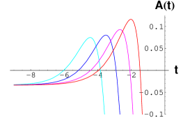
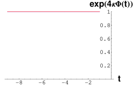
(a)                                     (b)                                     (c)

Figure 1: (a) $A(t)$ for $k_{b}=-1$ as a function of $t$ in the canonical case. The curves correspond to the cases with $t_{2}=t_{3}=-3,-2,-1,0$, according to the location of the peak from left to right. (b) $A(t)$ for $k_{b}=0$ as a function of $t$. The choice of parameters is the same as (a). (c) $\exp(4\kappa\Phi(t))=1$ is constant in this case. For the other parameters, see text.

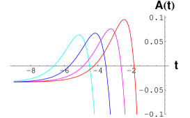
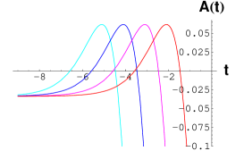
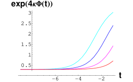
(a)                                     (b)                                     (c)

Figure 2: (a) $A(t)$ for $k_{b}=-1$ as a function of $t$ in the canonical case. The curves correspond to the cases with $t_{2}=-3,-2,-1,0$ and $t_{2}-t_{3}=1$, according to the location of the peak from left to right. (b) $A(t)$ for $k_{b}=0$ as a function of $t$. The choice of parameters is the same as (a). (c) $\exp(4\kappa\Phi(t))$ as a function of $t$. The color of the curve corresponds to (a). For the other parameters, see text.

We also find that if the value of $\alpha$ is sufficiently close to unity, there exists an accelerating phase for a wide range of $t_{2}-t_{1}$ and $t_{3}-t_{1}$. We conclude that the solution can give accelerating universes in the $(d+1)$-dimensional Einstein frame in the model with $\sigma=1$, $l>0$, $r>0$ and $k_{b}=-1$ and $k_{b}=0$. The result here is qualitatively similar to the result of Ref. Roy , where the dilaton coupling to a single flux term is considered.

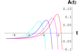
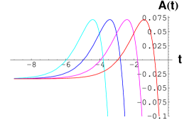
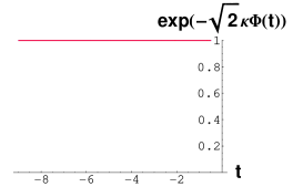
(a)                                     (b)                                     (c)

Figure 3: (a) $A(t)$ for $k_{b}=-1$ as a function of $t$ in the phantom case. The curves correspond to the cases with $t_{2}=t_{3}=-3,-2,-1,0$, according to the location of the peak from left to right. (b) $A(t)$ for $k_{b}=0$ as a function of $t$. The choice of parameters is the same as (a). (c) $\exp(-\sqrt{2}\kappa\Phi(t))=1$ is constant in this case. For the other parameters, see text.

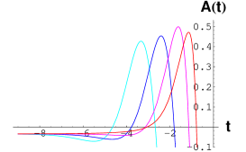
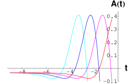
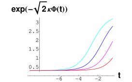
(a)                                     (b)                                     (c)

Figure 4: (a) $A(t)$ for $k_{b}=-1$ as a function of $t$ in the phantom case. The curves correspond to the cases with $t_{2}=-3,-2,-1,0$ and $t_{2}-t_{3}=1$, according to the location of the peak from left to right. (b) $A(t)$ for $k_{b}=0$ as a function of $t$. The choice of parameters is the same as (a). (c) $\exp(-\sqrt{2}\kappa\Phi(t))$ as a function of $t$. The color of the curve corresponds to (a). For the other parameters, see text.

A similar transient acceleration can be found in a special phantom case, $\sigma=-1$, $l>0$ and $r<0$, and ($E_{1}<0$, $E_{2}>0$, $E_{3}<0$). In this case, we choose the integration constant to satisfy $\lambda_{3}\sinh\theta=\lambda_{2}\cosh\theta$ in the solution (166) and obtain

$$e^{-2\kappa\left(\frac{1-\alpha^{2}}{\alpha}\right)\Phi(t)}=\frac{|r|}{l\alpha^{2}}\frac{\cosh^{2}[q\kappa(t-t_{3})]}{\cosh^{2}[q\kappa(t-t_{2})]}\,.$$ (119)

We now consider the simplest case, $D=6$, $d=3$, $l=-r=1$, $\alpha=1/\sqrt{2}$, $q=1$ and $t_{1}=0$. We show the values $A(t)$ versus $t$ for various values of $t_{2}$ and $t_{3}$ in Figs. 3 and 4 in this phantom case. It can be found that the acceleration period is later when $t_{2}-t_{3}$ is a larger positive value. Contrarily, negative $t_{2}-t_{3}$ leads to an earlier period of acceleration.

VI quantum cosmology

To study a very early universe and especially its initial state, we have to consider the quantum nature of cosmology. In our model, we can obtain the minisuperspace Wheeler–De Witt equation by replacing $\dot{x}_{a}\rightarrow-i\frac{\partial}{\partial x_{a}}$ (where we choose the natural unit $\hbar=1$) in the Hamiltonian $H$ and regarding the Hamiltonian constraint as $H\Psi=0$, where $\Psi$ is the wave function of the universe.

Our Hamiltonian becomes

$$H=\frac{1}{2}\frac{\partial^{2}}{\partial x^{2}}+\frac{V_{1}}{2}e^{2\lambda_{1}x}-\frac{1}{2}\frac{\partial^{2}}{\partial y^{2}}+\frac{lf^{2}}{2}e^{2\lambda_{2}y}-\frac{1}{2}\frac{\partial^{2}}{\partial z^{2}}+\frac{rf^{2}}{2}e^{2\lambda_{3}z}\quad\mbox{for}\quad\sigma=1\,,$$ (120)

$$H=\frac{1}{2}\frac{\partial^{2}}{\partial x^{2}}+\frac{V_{1}}{2}e^{2\lambda_{1}x}-\frac{1}{2}\frac{\partial^{2}}{\partial y^{2}}+\frac{lf^{2}}{2}e^{2\lambda_{2}y}+\frac{1}{2}\frac{\partial^{2}}{\partial z^{2}}+\frac{rf^{2}}{2}e^{2\lambda_{3}z}\quad\mbox{for}\quad\sigma=-1\,,$$ (121)

noticing that the definition of $\lambda_{2}$ and $\lambda_{3}$ is different in each case. Owing to the separation of variables, the wave function is expressed by superposition of the multiplicative form, $\Psi_{1}(x)\Psi_{2}(y)\Psi_{3}(z)$.

Let us first consider the case $\sigma=1$, $l>0$, and $r>0$. Then, the normalizable wave function can be written in the form

$$\Psi(x,y,z)=\int_{-\infty}^{\infty}dq\int_{0}^{2\pi}d\theta\,{\cal A}(q,\theta)\left[c_{1}F_{i\frac{q}{\lambda_{1}}}({\sqrt{V_{1}}}e^{\lambda_{1}x}/{\lambda_{1}})+c_{2}G_{i\frac{q}{\lambda_{1}}}({\sqrt{V_{1}}}e^{\lambda_{1}x}/{\lambda_{1}})\right]$$

$$\qquad\qquad\qquad\qquad\times\frac{2(\sqrt{l}f/(2\lambda_{2}))^{-iq\cos\theta/\lambda_{2}}}{\Gamma\left(-iq\cos\theta/\lambda_{2}\right)}K_{i\frac{q\cos\theta}{\lambda_{2}}}({\sqrt{l}f}e^{\lambda_{2}y}/{\lambda_{2}})$$

$$\qquad\qquad\qquad\qquad\times\frac{2(\sqrt{r}f/(2\lambda_{3}))^{-iq\sin\theta/\lambda_{3}}}{\Gamma\left(-iq\sin\theta/\lambda_{3}\right)}K_{i\frac{q\sin\theta}{\lambda_{3}}}({\sqrt{r}f}e^{\lambda_{3}z}/{\lambda_{3}})\,,$$ (122)

where ${\cal A}(q,\theta)$ is the amplitude and the eigenfunctions $F_{\nu}$ and $G_{\nu}$ are defined as ALNW ; Dunster

$$F_{\nu}(z)=\frac{1}{2\cos(\nu\pi/2)}[J_{\nu}(z)+J_{-\nu}(z)]\,,\quad G_{\nu}(z)=\frac{1}{2\sin(\nu\pi/2)}[J_{\nu}(z)-J_{-\nu}(z)]\,,$$ (123)

and $c_{1}$ and $c_{2}$ are constants. In this expression, we adopt the wave normalization found in Ref. LES1 , so

$$\frac{2(\sqrt{V}/(2\lambda))^{-iq/\lambda}}{\Gamma(-iq/\lambda)}K_{iq/\lambda}(\sqrt{V}e^{\lambda x}/\lambda)\sim e^{iqx}+R_{0}e^{-iqx}\,\quad\mbox{for}\quad x\rightarrow-\infty\,,$$ (124)

where $R_{0}=[\Gamma(iq/\lambda)/\Gamma(-iq/\lambda)](\sqrt{V}/(2\lambda))^{-2iq/\lambda}$.

The Gaussian wave packet is often considered ALNW ; KN ; Kiefer1 ; Kiefer2 ; DKS in a semiclassical analysis of quantum cosmology. There is another possibility that the amplitude ${\cal A}$ is independent of $\theta$, which is naturally motivated from the form of (122) because the integral region, or moduli space, of $\theta$ is apparently finite.

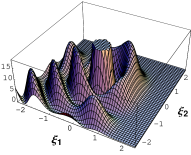
Figure 5: $|\psi_{q}(\xi_{1},\xi_{2})|^{2}$ with $q=4$.

To succinctly grasp what occurs by taking this assumption, we consider a simple calculation. We show $|\psi_{q}(\xi_{1},\xi_{2})|^{2}$ with $q=4$ in Fig. 5, where

$$\psi_{q}(\xi_{1},\xi_{2})\equiv\int_{0}^{2\pi}d\theta\,\frac{2(2)^{iq\cos\theta}}{\Gamma(-iq\cos\theta)}K_{i{q\cos\theta}}(e^{\xi_{1}})\frac{2(2)^{iq\sin\theta}}{\Gamma(-iq\sin\theta)}K_{i{q\sin\theta}}(e^{\xi_{2}})\,.$$ (125)

Many peaks of the function are located in the region $(\xi_{1}<0,\xi_{2}<0)$, and considerably high peaks are found at $\xi_{1}\sim\xi_{2}$. Because both the eigenfunction of $\xi_{1}$ and that of $\xi_{2}$ have the incoming wave and reflected wave from the potential wall, the interference of the four waves generates a complicated wave pattern. Nevertheless, we find that a chain of peaks appears in the line ${\xi_{1}}\sim{\xi_{2}}$, which seems plausible from symmetry.

From this fact, we expect that, if the amplitude ${\cal A}(q)$ is assumed to have a sufficiently narrow width, peaks of the probability density $|\Psi|^{2}$ appear at the discrete positions where ${\lambda_{2}y}\sim{\lambda_{3}z}$, i.e., $\Phi\sim 0$ for $\alpha\sim 1$. From the shape of the partial wave function, we can see that the initial state of the universe possesses a small but finite $e^{a}$, whose possible value is somewhat discretized, with the stationary value of $\Phi$.

Next, let us consider the phantom case $\sigma=-1$, $r<0$, and $k_{b}=1$. Then, the normalizable wave function can be written in the form

$$\Psi(x,y,z)=\int_{-\infty}^{\infty}dq\int_{0}^{2\pi}d\theta\,{\cal A}^{\prime}(q,\theta)\frac{2(\sqrt{V_{1}}/(2\lambda_{1}))^{-iq\cos\theta/\lambda_{1}}}{\Gamma(-iq\cos\theta/\lambda_{1})}K_{i\frac{q\cos\theta}{\lambda_{1}}}({\sqrt{|V_{1}|}}e^{\lambda_{1}x}/{\lambda_{1}})$$

$$\qquad\qquad\qquad\qquad\times\left[c_{1}F_{i\frac{q}{\lambda_{2}}}({\sqrt{l}f}e^{\lambda_{2}y}/{\lambda_{2}})+c_{2}G_{i\frac{q}{\lambda_{2}}}({\sqrt{l}f}e^{\lambda_{1}y}/{\lambda_{2}})\right]$$

$$\qquad\qquad\qquad\qquad\times\frac{2(\sqrt{|r|}f/(2\lambda_{3}))^{-iq\cos\theta/\lambda_{3}}}{\Gamma(-iq\cos\theta/\lambda_{3})}K_{i\frac{q\sin\theta}{\lambda_{3}}}({\sqrt{|r|}f}e^{\lambda_{3}z}/{\lambda_{3}})\,,$$ (126)

where ${\cal A}^{\prime}$ is the amplitude and we rearrange the integration constants.

We consider again the case ${\cal A}^{\prime}={\cal A}^{\prime}(q)$ as a Gaussian with a narrow width. As in the previous case, we expect high peaks at $\lambda_{1}x\sim\lambda_{3}z\lesssim 0$. Then, the initial state of the universe is equipped with some finite $e^{a}$ and $b\propto\Phi$.

The interpretation we present here is very qualitative, regrettably. To obtain more quantitative results, we should study the wave function carefully, by taking account of a normalization measure, which can be somewhat dependent on $\theta$, and a detailed calculation of the superposition. This study will be done in future work.

VII Summary and discussion

In this paper, a class of analytical cosmological solutions is considered in an integrable higher-dimensional model with a scalar field and an antisymmetric tensor field. The scalar field is either a canonical ($\sigma=+1$) or a phantom one ($\sigma=-1$).

In Sec. V, we looked for solutions for the accelerating universe. We found that the expanding universe with transient acceleration is obtained in the case with hyperbolic or flat internal space with positive energy density of the dilaton and antisymmetric fields ($\sigma=1$, $l>0$, and $r>0$), except for other special cases.

One of the special features of our model is that the value of $\Phi$ can be finite both at the beginning, $S\sim 0$, and at the far future of the universe, $\eta\rightarrow\infty$. The coupling between the dilaton field and additional gauge or matter fields can trigger some cosmological time-dependent phenomena, though, unfortunately, it is difficult to interpret the present fields in the $(d+1)$-dimensional universe. The study of the inclusion of matter fields is significant in any case, even apart from pursuing exact solutions.

We briefly argued the quantum cosmology of some specific cases. Throughout this paper, we found that separable variables made the analyses simple, both in the classical and the quantum cosmological behavior of the scale factor. However, further deeper investigation is required, especially for cosmology with initial bouncing behavior, which has not been discussed in the present study. We should also consider various aspects of wave functions of the universe in our model in a more precise manner. We leave these subjects for future work.

Appendix A Summary of solutions

Here, we summarize the solutions and show the expressions for two scale factors $a$ and $b$ and the scalar field $\Phi$. They are found by using $x$, $y$, and $z$, as follows:

$$e^{2da(t)}=\left(e^{2\lambda_{2}y}\right)^{\frac{\sigma}{\alpha^{2}+\sigma}}\left(e^{2\lambda_{3}z}\right)^{\frac{\alpha^{2}}{\alpha^{2}+\sigma}}\,,$$ (127)

$$e^{2(D-d-2)b(t)}=e^{2\lambda_{1}x}\left(e^{2\lambda_{2}y}\right)^{-\frac{\sigma}{\alpha^{2}+\sigma}}\left(e^{2\lambda_{3}z}\right)^{-\frac{\alpha^{2}}{\alpha^{2}+\sigma}}\,,$$ (128)

$$e^{2\kappa\Phi(t)}=\left(\frac{e^{2\lambda_{2}y}}{e^{2\lambda_{3}z}}\right)^{\frac{\alpha}{\alpha^{2}+\sigma}}\,.$$ (129)

We exhibit them by categorizing the sign of $\sigma$, the signs of $l$ and $r$, and the values for $k_{b}$, in this order. In the following expressions, $t_{1}$, $t_{2}$, $t_{3}$, $q$, and $\theta$ are integration constants.

A.1 $\sigma=+1$

A.1.1 $l>0$ and $r>0$ ($E_{1}<0$, $E_{2}>0$, $E_{3}>0$)

• $k_{b}=-1$

  $$e^{2da(t)}=\frac{1}{f^{2}}\left(\frac{q^{2}\cos^{2}\theta}{l\cosh^{2}[q\cos\theta\lambda_{2}(t-t_{2})]}\right)^{\frac{1}{\alpha^{2}+1}}\left(\frac{q^{2}\sin^{2}\theta}{r\cosh^{2}[q\sin\theta\lambda_{3}(t-t_{3})]}\right)^{\frac{\alpha^{2}}{\alpha^{2}+1}}\,,$$

  $$e^{2(D-d-2)b(t)}=\frac{f^{2}q^{2}}{V_{1}\sinh^{2}[q\lambda_{1}(t-t_{1})]}\left(\frac{q^{2}\cos^{2}\theta}{l\cosh^{2}[q\cos\theta\lambda_{2}(t-t_{2})]}\right)^{-\frac{1}{\alpha^{2}+1}}\left(\frac{q^{2}\sin^{2}\theta}{r\cosh^{2}[q\sin\theta\lambda_{3}(t-t_{3})]}\right)^{-\frac{\alpha^{2}}{\alpha^{2}+1}}\,,$$

  $$e^{2\kappa\Phi(t)}=\left(\frac{r\cos^{2}\theta}{l\sin^{2}\theta}\frac{\cosh^{2}[q\sin\theta\lambda_{3}(t-t_{3})]}{\cosh^{2}[q\cos\theta\lambda_{2}(t-t_{2})]}\right)^{\frac{\alpha}{\alpha^{2}+1}}\,.$$ (130)

• $k_{b}=0$

  $$e^{2da(t)}=\frac{1}{f^{2}}\left(\frac{q^{2}\cos^{2}\theta}{l\cosh^{2}[q\cos\theta\lambda_{2}(t-t_{2})]}\right)^{\frac{1}{\alpha^{2}+1}}\left(\frac{q^{2}\sin^{2}\theta}{r\cosh^{2}[q\sin\theta\lambda_{3}(t-t_{3})]}\right)^{\frac{\alpha^{2}}{\alpha^{2}+1}}\,,$$

  $$e^{2(D-d-2)b(t)}=C_{1}f^{2}e^{2\lambda_{1}qt}\left(\frac{q^{2}\cos^{2}\theta}{l\cosh^{2}[q\cos\theta\lambda_{2}(t-t_{2})]}\right)^{-\frac{1}{\alpha^{2}+1}}\left(\frac{q^{2}\sin^{2}\theta}{r\cosh^{2}[q\sin\theta\lambda_{3}(t-t_{3})]}\right)^{-\frac{\alpha^{2}}{\alpha^{2}+1}}\,,$$

  $$e^{2\kappa\Phi(t)}=\left(\frac{r\cos^{2}\theta}{l\sin^{2}\theta}\frac{\cosh^{2}[q\sin\theta\lambda_{3}(t-t_{3})]}{\cosh^{2}[q\cos\theta\lambda_{2}(t-t_{2})]}\right)^{\frac{\alpha}{\alpha^{2}+1}}\,,$$ (131)

  where we define $C_{1}\equiv e^{-2q\lambda_{1}t_{1}}$. Hereafter, we use this definition.

• $k_{b}=+1$

  $$e^{2da(t)}=\frac{1}{f^{2}}\left(\frac{q^{2}\cos^{2}\theta}{l\cosh^{2}[q\cos\theta\lambda_{2}(t-t_{2})]}\right)^{\frac{1}{\alpha^{2}+1}}\left(\frac{q^{2}\sin^{2}\theta}{r\cosh^{2}[q\sin\theta\lambda_{3}(t-t_{3})]}\right)^{\frac{\alpha^{2}}{\alpha^{2}+1}}\,,$$

  $$e^{2(D-d-2)b(t)}=\frac{f^{2}q^{2}}{|V_{1}|\cosh^{2}[q\lambda_{1}(t-t_{1})]}\left(\frac{q^{2}\cos^{2}\theta}{l\cosh^{2}[q\cos\theta\lambda_{2}(t-t_{2})]}\right)^{-\frac{1}{\alpha^{2}+1}}\left(\frac{q^{2}\sin^{2}\theta}{r\cosh^{2}[q\sin\theta\lambda_{3}(t-t_{3})]}\right)^{-\frac{\alpha^{2}}{\alpha^{2}+1}}\,,$$

  $$e^{2\kappa\Phi(t)}=\left(\frac{r\cos^{2}\theta}{l\sin^{2}\theta}\frac{\cosh^{2}[q\sin\theta\lambda_{3}(t-t_{3})]}{\cosh^{2}[q\cos\theta\lambda_{2}(t-t_{2})]}\right)^{\frac{\alpha}{\alpha^{2}+1}}\,.$$ (132)

A.1.2 $l>0$ and $r<0$

• $k_{b}=-1$

  (I) $$~{}(E_{1}<0,E_{2}>0,E_{3}>0)$$ (133)

  $$e^{2da(t)}=\frac{1}{f^{2}}\left(\frac{q^{2}\cos^{2}\theta}{l\cosh^{2}[q\cos\theta\lambda_{2}(t-t_{2})]}\right)^{\frac{1}{\alpha^{2}+1}}\left(\frac{q^{2}\sin^{2}\theta}{|r|\sinh^{2}[q\sin\theta\lambda_{3}(t-t_{3})]}\right)^{\frac{\alpha^{2}}{\alpha^{2}+1}}\,,$$

  $$e^{2(D-d-2)b(t)}=\frac{f^{2}q^{2}}{V_{1}\sinh^{2}[q\lambda_{1}(t-t_{1})]}\left(\frac{q^{2}\cos^{2}\theta}{l\cosh^{2}[q\cos\theta\lambda_{2}(t-t_{2})]}\right)^{-\frac{1}{\alpha^{2}+1}}\left(\frac{q^{2}\sin^{2}\theta}{|r|\sinh^{2}[q\sin\theta\lambda_{3}(t-t_{3})]}\right)^{-\frac{\alpha^{2}}{\alpha^{2}+1}}\,,$$

  $$e^{2\kappa\Phi(t)}=\left(\frac{|r|\cos^{2}\theta}{l\sin^{2}\theta}\frac{\sinh^{2}[q\sin\theta\lambda_{3}(t-t_{3})]}{\cosh^{2}[q\cos\theta\lambda_{2}(t-t_{2})]}\right)^{\frac{\alpha}{\alpha^{2}+1}}\,.$$

  (II) $$~{}(E_{1}<0,E_{2}>0,E_{3}<0)$$ (134)

  $$e^{2da(t)}=\frac{1}{f^{2}}\left(\frac{q^{2}\cosh^{2}\theta}{l\cosh^{2}[q\cosh\theta\lambda_{2}(t-t_{2})]}\right)^{\frac{1}{\alpha^{2}+1}}\left(\frac{q^{2}\sinh^{2}\theta}{|r|\sin^{2}[q\sinh\theta\lambda_{3}(t-t_{3})]}\right)^{\frac{\alpha^{2}}{\alpha^{2}+1}}\,,$$

  $$e^{2(D-d-2)b(t)}=\frac{f^{2}q^{2}}{V_{1}\sinh^{2}[q\lambda_{1}(t-t_{1})]}\left(\frac{q^{2}\cosh^{2}\theta}{l\cosh^{2}[q\cosh\theta\lambda_{2}(t-t_{2})]}\right)^{-\frac{1}{\alpha^{2}+1}}\left(\frac{q^{2}\sinh^{2}\theta}{|r|\sin^{2}[q\sinh\theta\lambda_{3}(t-t_{3})]}\right)^{-\frac{\alpha^{2}}{\alpha^{2}+1}}\,,$$

  $$e^{2\kappa\Phi(t)}=\left(\frac{|r|\cosh^{2}\theta}{l\sinh^{2}\theta}\frac{\sin^{2}[q\sinh\theta\lambda_{3}(t-t_{3})]}{\cosh^{2}[q\cosh\theta\lambda_{2}(t-t_{2})]}\right)^{\frac{\alpha}{\alpha^{2}+1}}\,.$$

  (III) $$~{}(E_{1}>0,E_{2}>0,E_{3}<0)$$ (135)

  $$e^{2da(t)}=\frac{1}{f^{2}}\left(\frac{q^{2}\sinh^{2}\theta}{l\cosh^{2}[q\sinh\theta\lambda_{2}(t-t_{2})]}\right)^{\frac{1}{\alpha^{2}+1}}\left(\frac{q^{2}\cosh^{2}\theta}{|r|\sin^{2}[q\cosh\theta\lambda_{3}(t-t_{3})]}\right)^{\frac{\alpha^{2}}{\alpha^{2}+1}}\,,$$

  $$e^{2(D-d-2)b(t)}=\frac{f^{2}q^{2}}{V_{1}\sin^{2}[q\lambda_{1}(t-t_{1})]}\left(\frac{q^{2}\sinh^{2}\theta}{l\cosh^{2}[q\sinh\theta\lambda_{2}(t-t_{2})]}\right)^{-\frac{1}{\alpha^{2}+1}}\left(\frac{q^{2}\cosh^{2}\theta}{|r|\sin^{2}[q\cosh\theta\lambda_{3}(t-t_{3})]}\right)^{-\frac{\alpha^{2}}{\alpha^{2}+1}}\,,$$

  $$e^{2\kappa\Phi(t)}=\left(\frac{|r|\sinh^{2}\theta}{l\cosh^{2}\theta}\frac{\sin^{2}[q\cosh\theta\lambda_{3}(t-t_{3})]}{\cosh^{2}[q\sinh\theta\lambda_{2}(t-t_{2})]}\right)^{\frac{\alpha}{\alpha^{2}+1}}\,.$$

• $k_{b}=0$

  (I) $$~{}(E_{1}<0,E_{2}>0,E_{3}>0)$$ (136)

  $$e^{2da(t)}=\frac{1}{f^{2}}\left(\frac{q^{2}\cos^{2}\theta}{l\cosh^{2}[q\cos\theta\lambda_{2}(t-t_{2})]}\right)^{\frac{1}{\alpha^{2}+1}}\left(\frac{q^{2}\sin^{2}\theta}{|r|\sinh^{2}[q\sin\theta\lambda_{3}(t-t_{3})]}\right)^{\frac{\alpha^{2}}{\alpha^{2}+1}}\,,$$

  $$e^{2(D-d-2)b(t)}=C_{1}f^{2}e^{2\lambda_{1}qt}\left(\frac{q^{2}\cos^{2}\theta}{l\cosh^{2}[q\cos\theta\lambda_{2}(t-t_{2})]}\right)^{-\frac{1}{\alpha^{2}+1}}\left(\frac{q^{2}\sin^{2}\theta}{|r|\sinh^{2}[q\sin\theta\lambda_{3}(t-t_{3})]}\right)^{-\frac{\alpha^{2}}{\alpha^{2}+1}}\,,$$

  $$e^{2\kappa\Phi(t)}=\left(\frac{|r|\cos^{2}\theta}{l\sin^{2}\theta}\frac{\sinh^{2}[q\sin\theta\lambda_{3}(t-t_{3})]}{\cosh^{2}[q\cos\theta\lambda_{2}(t-t_{2})]}\right)^{\frac{\alpha}{\alpha^{2}+1}}\,.$$

  (II) $$~{}(E_{1}<0,E_{2}>0,E_{3}<0)$$ (137)

  $$e^{2da(t)}=\frac{1}{f^{2}}\left(\frac{q^{2}\cosh^{2}\theta}{l\cosh^{2}[q\cosh\theta\lambda_{2}(t-t_{2})]}\right)^{\frac{1}{\alpha^{2}+1}}\left(\frac{q^{2}\sinh^{2}\theta}{|r|\sin^{2}[q\sinh\theta\lambda_{3}(t-t_{3})]}\right)^{\frac{\alpha^{2}}{\alpha^{2}+1}}\,,$$

  $$e^{2(D-d-2)b(t)}=f^{2}e^{2\lambda_{1}q(t-t_{1})}\left(\frac{q^{2}\cosh^{2}\theta}{l\cosh^{2}[q\cosh\theta\lambda_{2}(t-t_{2})]}\right)^{-\frac{1}{\alpha^{2}+1}}\left(\frac{q^{2}\sinh^{2}\theta}{|r|\sin^{2}[q\sinh\theta\lambda_{3}(t-t_{3})]}\right)^{-\frac{\alpha^{2}}{\alpha^{2}+1}}\,,$$

  $$e^{2\kappa\Phi(t)}=\left(\frac{|r|\cosh^{2}\theta}{l\sinh^{2}\theta}\frac{\sin^{2}[q\sinh\theta\lambda_{3}(t-t_{3})]}{\cosh^{2}[q\cosh\theta\lambda_{2}(t-t_{2})]}\right)^{\frac{\alpha}{\alpha^{2}+1}}\,.$$

• $k_{b}=+1$

  (I) $$~{}(E_{1}<0,E_{2}>0,E_{3}>0)$$ (138)

  $$e^{2da(t)}=\frac{1}{f^{2}}\left(\frac{q^{2}\cos^{2}\theta}{l\cosh^{2}[q\cos\theta\lambda_{2}(t-t_{2})]}\right)^{\frac{1}{\alpha^{2}+1}}\left(\frac{q^{2}\sin^{2}\theta}{|r|\sinh^{2}[q\sin\theta\lambda_{3}(t-t_{3})]}\right)^{\frac{\alpha^{2}}{\alpha^{2}+1}}\,,$$

  $$e^{2(D-d-2)b(t)}=\frac{f^{2}q^{2}}{|V_{1}|\cosh^{2}[q\lambda_{1}(t-t_{1})]}\left(\frac{q^{2}\cos^{2}\theta}{l\cosh^{2}[q\cos\theta\lambda_{2}(t-t_{2})]}\right)^{-\frac{1}{\alpha^{2}+1}}\left(\frac{q^{2}\sin^{2}\theta}{|r|\sinh^{2}[q\sin\theta\lambda_{3}(t-t_{3})]}\right)^{-\frac{\alpha^{2}}{\alpha^{2}+1}}\,,$$

  $$e^{2\kappa\Phi(t)}=\left(\frac{|r|\cos^{2}\theta}{l\sin^{2}\theta}\frac{\sinh^{2}[q\sin\theta\lambda_{3}(t-t_{3})]}{\cosh^{2}[q\cos\theta\lambda_{2}(t-t_{2})]}\right)^{\frac{\alpha}{\alpha^{2}+1}}\,.$$

  (II) $$~{}(E_{1}<0,E_{2}>0,E_{3}<0)$$ (139)

  $$e^{2da(t)}=\frac{1}{f^{2}}\left(\frac{q^{2}\cosh^{2}\theta}{l\cosh^{2}[q\cosh\theta\lambda_{2}(t-t_{2})]}\right)^{\frac{1}{\alpha^{2}+1}}\left(\frac{q^{2}\sinh^{2}\theta}{|r|\sin^{2}[q\sinh\theta\lambda_{3}(t-t_{3})]}\right)^{\frac{\alpha^{2}}{\alpha^{2}+1}}\,,$$

  $$e^{2(D-d-2)b(t)}=\frac{f^{2}q^{2}}{|V_{1}|\cosh^{2}[q\lambda_{1}(t-t_{1})]}\left(\frac{q^{2}\cosh^{2}\theta}{l\cosh^{2}[q\cosh\theta\lambda_{2}(t-t_{2})]}\right)^{-\frac{1}{\alpha^{2}+1}}\left(\frac{q^{2}\sinh^{2}\theta}{|r|\sin^{2}[q\sinh\theta\lambda_{3}(t-t_{3})]}\right)^{-\frac{\alpha^{2}}{\alpha^{2}+1}}\,,$$

  $$e^{2\kappa\Phi(t)}=\left(\frac{|r|\cosh^{2}\theta}{l\sinh^{2}\theta}\frac{\sin^{2}[q\sin\theta\lambda_{3}(t-t_{3})]}{\cosh^{2}[q\cosh\theta\lambda_{2}(t-t_{2})]}\right)^{\frac{\alpha}{\alpha^{2}+1}}\,.$$

A.1.3 $l<0$ and $r>0$

• $k_{b}=-1$

  (I) $$~{}(E_{1}<0,E_{2}>0,E_{3}>0)$$ (140)

  $$e^{2da(t)}=\frac{1}{f^{2}}\left(\frac{q^{2}\cos^{2}\theta}{|l|\sinh^{2}[q\cos\theta\lambda_{2}(t-t_{2})]}\right)^{\frac{1}{\alpha^{2}+1}}\left(\frac{q^{2}\sin^{2}\theta}{r\cosh^{2}[q\sin\theta\lambda_{3}(t-t_{3})]}\right)^{\frac{\alpha^{2}}{\alpha^{2}+1}}\,,$$

  $$e^{2(D-d-2)b(t)}=\frac{f^{2}q^{2}}{V_{1}\sinh^{2}[q\lambda_{1}(t-t_{1})]}\left(\frac{q^{2}\cos^{2}\theta}{|l|\sinh^{2}[q\cos\theta\lambda_{2}(t-t_{2})]}\right)^{-\frac{1}{\alpha^{2}+1}}\left(\frac{q^{2}\sin^{2}\theta}{r\cosh^{2}[q\sin\theta\lambda_{3}(t-t_{3})]}\right)^{-\frac{\alpha^{2}}{\alpha^{2}+1}}\,,$$

  $$e^{2\kappa\Phi(t)}=\left(\frac{r\cos^{2}\theta}{|l|\sin^{2}\theta}\frac{\cosh^{2}[q\sin\theta\lambda_{3}(t-t_{3})]}{\sinh^{2}[q\cos\theta\lambda_{2}(t-t_{2})]}\right)^{\frac{\alpha}{\alpha^{2}+1}}\,.$$

  (II) $$~{}(E_{1}<0,E_{2}<0,E_{3}>0)$$ (141)

  $$e^{2da(t)}=\frac{1}{f^{2}}\left(\frac{q^{2}\sinh^{2}\theta}{|l|\sin^{2}[q\sinh\theta\lambda_{2}(t-t_{2})]}\right)^{\frac{1}{\alpha^{2}+1}}\left(\frac{q^{2}\cosh^{2}\theta}{r\cosh^{2}[q\cosh\theta\lambda_{3}(t-t_{3})]}\right)^{\frac{\alpha^{2}}{\alpha^{2}+1}}\,,$$

  $$e^{2(D-d-2)b(t)}=\frac{f^{2}q^{2}}{V_{1}\sinh^{2}[q\lambda_{1}(t-t_{1})]}\left(\frac{q^{2}\sinh^{2}\theta}{|l|\sin^{2}[q\sinh\theta\lambda_{2}(t-t_{2})]}\right)^{-\frac{1}{\alpha^{2}+1}}\left(\frac{q^{2}\cosh^{2}\theta}{r\cosh^{2}[q\cosh\theta\lambda_{3}(t-t_{3})]}\right)^{-\frac{\alpha^{2}}{\alpha^{2}+1}}\,,$$

  $$e^{2\kappa\Phi(t)}=\left(\frac{r\sinh^{2}\theta}{|l|\cosh^{2}\theta}\frac{\cosh^{2}[q\cosh\theta\lambda_{3}(t-t_{3})]}{\sin^{2}[q\sinh\theta\lambda_{2}(t-t_{2})]}\right)^{\frac{\alpha}{\alpha^{2}+1}}\,.$$

  (III) $$~{}(E_{1}>0,E_{2}<0,E_{3}>0)$$ (142)

  $$e^{2da(t)}=\frac{1}{f^{2}}\left(\frac{q^{2}\cosh^{2}\theta}{|l|\sin^{2}[q\cosh\theta\lambda_{2}(t-t_{2})]}\right)^{\frac{1}{\alpha^{2}+1}}\left(\frac{q^{2}\sinh^{2}\theta}{r\cosh^{2}[q\sinh\theta\lambda_{3}(t-t_{3})]}\right)^{\frac{\alpha^{2}}{\alpha^{2}+1}}\,,$$

  $$e^{2(D-d-2)b(t)}=\frac{f^{2}q^{2}}{V_{1}\sin^{2}[q\lambda_{1}(t-t_{1})]}\left(\frac{q^{2}\cosh^{2}\theta}{|l|\sin^{2}[q\cosh\theta\lambda_{2}(t-t_{2})]}\right)^{-\frac{1}{\alpha^{2}+1}}\left(\frac{q^{2}\sinh^{2}\theta}{r\cosh^{2}[q\sinh\theta\lambda_{3}(t-t_{3})]}\right)^{-\frac{\alpha^{2}}{\alpha^{2}+1}}\,,$$

  $$e^{2\kappa\Phi(t)}=\left(\frac{r\cosh^{2}\theta}{|l|\sinh^{2}\theta}\frac{\cosh^{2}[q\sinh\theta\lambda_{3}(t-t_{3})]}{\sin^{2}[q\cosh\theta\lambda_{2}(t-t_{2})]}\right)^{\frac{\alpha}{\alpha^{2}+1}}\,.$$

• $k_{b}=0$

  (I) $$~{}(E_{1}<0,E_{2}>0,E_{3}>0)$$ (143)

  $$e^{2da(t)}=\frac{1}{f^{2}}\left(\frac{q^{2}\cos^{2}\theta}{|l|\sinh^{2}[q\cos\theta\lambda_{2}(t-t_{2})]}\right)^{\frac{1}{\alpha^{2}+1}}\left(\frac{q^{2}\sin^{2}\theta}{r\cosh^{2}[q\sin\theta\lambda_{3}(t-t_{3})]}\right)^{\frac{\alpha^{2}}{\alpha^{2}+1}}\,,$$

  $$e^{2(D-d-2)b(t)}=C_{1}f^{2}e^{2q\lambda_{1}t}\left(\frac{q^{2}\cos^{2}\theta}{|l|\sinh^{2}[q\cos\theta\lambda_{2}(t-t_{2})]}\right)^{-\frac{1}{\alpha^{2}+1}}\left(\frac{q^{2}\sin^{2}\theta}{r\cosh^{2}[q\sin\theta\lambda_{3}(t-t_{3})]}\right)^{-\frac{\alpha^{2}}{\alpha^{2}+1}}\,,$$

  $$e^{2\kappa\Phi(t)}=\left(\frac{r\cos^{2}\theta}{|l|\sin^{2}\theta}\frac{\cosh^{2}[q\sin\theta\lambda_{3}(t-t_{3})]}{\sinh^{2}[q\cos\theta\lambda_{2}(t-t_{2})]}\right)^{\frac{\alpha}{\alpha^{2}+1}}\,.$$

  (II) $$~{}(E_{1}<0,E_{2}<0,E_{3}>0)$$ (144)

  $$e^{2da(t)}=\frac{1}{f^{2}}\left(\frac{q^{2}\sinh^{2}\theta}{|l|\sin^{2}[q\sinh\theta\lambda_{2}(t-t_{2})]}\right)^{\frac{1}{\alpha^{2}+1}}\left(\frac{q^{2}\cosh^{2}\theta}{r\cosh^{2}[q\cosh\theta\lambda_{3}(t-t_{3})]}\right)^{\frac{\alpha^{2}}{\alpha^{2}+1}}\,,$$

  $$e^{2(D-d-2)b(t)}=f^{2}e^{2q\lambda_{1}(t-t_{1})}\left(\frac{q^{2}\sinh^{2}\theta}{|l|\sin^{2}[q\sinh\theta\lambda_{2}(t-t_{2})]}\right)^{-\frac{1}{\alpha^{2}+1}}\left(\frac{q^{2}\cosh^{2}\theta}{r\cosh^{2}[q\cosh\theta\lambda_{3}(t-t_{3})]}\right)^{-\frac{\alpha^{2}}{\alpha^{2}+1}}\,,$$

  $$e^{2\kappa\Phi(t)}=\left(\frac{r\sinh^{2}\theta}{|l|\cosh^{2}\theta}\frac{\cosh^{2}[q\cosh\theta\lambda_{3}(t-t_{3})]}{\sin^{2}[q\sinh\theta\lambda_{2}(t-t_{2})]}\right)^{\frac{\alpha}{\alpha^{2}+1}}\,.$$

• $k_{b}=+1$

  (I) $$~{}(E_{1}<0,E_{2}>0,E_{3}>0)$$ (145)

  $$e^{2da(t)}=\frac{1}{f^{2}}\left(\frac{q^{2}\cos^{2}\theta}{|l|\sinh^{2}[q\cos\theta\lambda_{2}(t-t_{2})]}\right)^{\frac{1}{\alpha^{2}+1}}\left(\frac{q^{2}\sin^{2}\theta}{r\cosh^{2}[q\sin\theta\lambda_{3}(t-t_{3})]}\right)^{\frac{\alpha^{2}}{\alpha^{2}+1}}\,,$$

  $$e^{2(D-d-2)b(t)}=\frac{f^{2}q^{2}}{|V_{1}|\cosh^{2}[q\lambda_{1}(t-t_{1})]}\left(\frac{q^{2}\cos^{2}\theta}{|l|\sinh^{2}[q\cos\theta\lambda_{2}(t-t_{2})]}\right)^{-\frac{1}{\alpha^{2}+1}}\left(\frac{q^{2}\sin^{2}\theta}{r\cosh^{2}[q\sin\theta\lambda_{3}(t-t_{3})]}\right)^{-\frac{\alpha^{2}}{\alpha^{2}+1}}\,,$$

  $$e^{2\kappa\Phi(t)}=\left(\frac{r\cos^{2}\theta}{|l|\sin^{2}\theta}\frac{\cosh^{2}[q\sin\theta\lambda_{3}(t-t_{3})]}{\sinh^{2}[q\cos\theta\lambda_{2}(t-t_{2})]}\right)^{\frac{\alpha}{\alpha^{2}+1}}\,.$$

  (II) $$~{}(E_{1}<0,E_{2}<0,E_{3}>0)$$ (146)

  $$e^{2da(t)}=\frac{1}{f^{2}}\left(\frac{q^{2}\sinh^{2}\theta}{|l|\sin^{2}[q\sinh\theta\lambda_{2}(t-t_{2})]}\right)^{\frac{1}{\alpha^{2}+1}}\left(\frac{q^{2}\cosh^{2}\theta}{r\cosh^{2}[q\cosh\theta\lambda_{3}(t-t_{3})]}\right)^{\frac{\alpha^{2}}{\alpha^{2}+1}}\,,$$

  $$e^{2(D-d-2)b(t)}=\frac{f^{2}q^{2}}{|V_{1}|\cosh^{2}[q\lambda_{1}(t-t_{1})]}\left(\frac{q^{2}\sinh^{2}\theta}{|l|\sin^{2}[q\sinh\theta\lambda_{2}(t-t_{2})]}\right)^{-\frac{1}{\alpha^{2}+1}}\left(\frac{q^{2}\cosh^{2}\theta}{r\cosh^{2}[q\cosh\theta\lambda_{3}(t-t_{3})]}\right)^{-\frac{\alpha^{2}}{\alpha^{2}+1}}\,,$$

  $$e^{2\kappa\Phi(t)}=\left(\frac{r\sinh^{2}\theta}{|l|\cosh^{2}\theta}\frac{\cosh^{2}[q\cosh\theta\lambda_{3}(t-t_{3})]}{\sin^{2}[q\sinh\theta\lambda_{2}(t-t_{2})]}\right)^{\frac{\alpha}{\alpha^{2}+1}}\,.$$

A.1.4 $l<0$ and $r<0$

• $k_{b}=-1$

  (I) $$~{}(E_{1}<0,E_{2}>0,E_{3}>0)$$ (147)

  $$e^{2da(t)}=\frac{1}{f^{2}}\left(\frac{q^{2}\cos^{2}\theta}{|l|\sinh^{2}[q\cos\theta\lambda_{2}(t-t_{2})]}\right)^{\frac{1}{\alpha^{2}+1}}\left(\frac{q^{2}\sin^{2}\theta}{|r|\sinh^{2}[q\sin\theta\lambda_{3}(t-t_{3})]}\right)^{\frac{\alpha^{2}}{\alpha^{2}+1}}\,,$$

  $$e^{2(D-d-2)b(t)}=\frac{f^{2}q^{2}}{V_{1}\sinh^{2}[q\lambda_{1}(t-t_{1})]}\left(\frac{q^{2}\cos^{2}\theta}{|l|\sinh^{2}[q\cos\theta\lambda_{2}(t-t_{2})]}\right)^{-\frac{1}{\alpha^{2}+1}}\left(\frac{q^{2}\sin^{2}\theta}{|r|\sinh^{2}[q\sin\theta\lambda_{3}(t-t_{3})]}\right)^{-\frac{\alpha^{2}}{\alpha^{2}+1}}\,,$$

  $$e^{2\kappa\Phi(t)}=\left(\frac{|r|\cos^{2}\theta}{|l|\sin^{2}\theta}\frac{\sinh^{2}[q\sin\theta\lambda_{3}(t-t_{3})]}{\sinh^{2}[q\cos\theta\lambda_{2}(t-t_{2})]}\right)^{\frac{\alpha}{\alpha^{2}+1}}\,.$$

  (II) $$~{}(E_{1}<0,E_{2}>0,E_{3}<0)$$ (148)

  $$e^{2da(t)}=\frac{1}{f^{2}}\left(\frac{q^{2}\cosh^{2}\theta}{|l|\sinh^{2}[q\cosh\theta\lambda_{2}(t-t_{2})]}\right)^{\frac{1}{\alpha^{2}+1}}\left(\frac{q^{2}\sinh^{2}\theta}{|r|\sin^{2}[q\sinh\theta\lambda_{3}(t-t_{3})]}\right)^{\frac{\alpha^{2}}{\alpha^{2}+1}}\,,$$

  $$e^{2(D-d-2)b(t)}=\frac{f^{2}q^{2}}{V_{1}\sinh^{2}[q\lambda_{1}(t-t_{1})]}\left(\frac{q^{2}\cosh^{2}\theta}{|l|\sinh^{2}[q\cosh\theta\lambda_{2}(t-t_{2})]}\right)^{-\frac{1}{\alpha^{2}+1}}\left(\frac{q^{2}\sinh^{2}\theta}{|r|\sin^{2}[q\sinh\theta\lambda_{3}(t-t_{3})]}\right)^{-\frac{\alpha^{2}}{\alpha^{2}+1}}\,,$$

  $$e^{2\kappa\Phi(t)}=\left(\frac{|r|\cosh^{2}\theta}{|l|\sinh^{2}\theta}\frac{\sin^{2}[q\sinh\theta\lambda_{3}(t-t_{3})]}{\sinh^{2}[q\cosh\theta\lambda_{2}(t-t_{2})]}\right)^{\frac{\alpha}{\alpha^{2}+1}}\,.$$

  (III) $$~{}(E_{1}<0,E_{2}<0,E_{3}>0)$$ (149)

  $$e^{2da(t)}=\frac{1}{f^{2}}\left(\frac{q^{2}\sinh^{2}\theta}{|l|\sin^{2}[q\sinh\theta\lambda_{2}(t-t_{2})]}\right)^{\frac{1}{\alpha^{2}+1}}\left(\frac{q^{2}\cosh^{2}\theta}{|r|\sinh^{2}[q\cosh\theta\lambda_{3}(t-t_{3})]}\right)^{\frac{\alpha^{2}}{\alpha^{2}+1}}\,,$$

  $$e^{2(D-d-2)b(t)}=\frac{f^{2}q^{2}}{V_{1}\sinh^{2}[q\lambda_{1}(t-t_{1})]}\left(\frac{q^{2}\sinh^{2}\theta}{|l|\sin^{2}[q\sinh\theta\lambda_{2}(t-t_{2})]}\right)^{-\frac{1}{\alpha^{2}+1}}\left(\frac{q^{2}\cosh^{2}\theta}{|r|\sinh^{2}[q\cosh\theta\lambda_{3}(t-t_{3})]}\right)^{-\frac{\alpha^{2}}{\alpha^{2}+1}}\,,$$

  $$e^{2\kappa\Phi(t)}=\left(\frac{|r|\sinh^{2}\theta}{|l|\cosh^{2}\theta}\frac{\sinh^{2}[q\cosh\theta\lambda_{3}(t-t_{3})]}{\sin^{2}[q\sinh\theta\lambda_{2}(t-t_{2})]}\right)^{\frac{\alpha}{\alpha^{2}+1}}\,.$$

  (IV) $$~{}(E_{1}>0,E_{2}<0,E_{3}<0)$$ (150)

  $$e^{2da(t)}=\frac{1}{f^{2}}\left(\frac{q^{2}\cos^{2}\theta}{|l|\sin^{2}[q\cos\theta\lambda_{2}(t-t_{2})]}\right)^{\frac{1}{\alpha^{2}+1}}\left(\frac{q^{2}\sin^{2}\theta}{|r|\sin^{2}[q\sin\theta\lambda_{3}(t-t_{3})]}\right)^{\frac{\alpha^{2}}{\alpha^{2}+1}}\,,$$

  $$e^{2(D-d-2)b(t)}=\frac{f^{2}q^{2}}{V_{1}\sin^{2}[q\lambda_{1}(t-t_{1})]}\left(\frac{q^{2}\cos^{2}\theta}{|l|\sin^{2}[q\cos\theta\lambda_{2}(t-t_{2})]}\right)^{-\frac{1}{\alpha^{2}+1}}\left(\frac{q^{2}\sin^{2}\theta}{|r|\sin^{2}[q\sin\theta\lambda_{3}(t-t_{3})]}\right)^{-\frac{\alpha^{2}}{\alpha^{2}+1}}\,,$$

  $$e^{2\kappa\Phi(t)}=\left(\frac{|r|\cos^{2}\theta}{|l|\sin^{2}\theta}\frac{\sin^{2}[q\sin\theta\lambda_{3}(t-t_{3})]}{\sin^{2}[q\cos\theta\lambda_{2}(t-t_{2})]}\right)^{\frac{\alpha}{\alpha^{2}+1}}\,.$$

  (V) $$~{}(E_{1}>0,E_{2}>0,E_{3}<0)$$ (151)

  $$e^{2da(t)}=\frac{1}{f^{2}}\left(\frac{q^{2}\sinh^{2}\theta}{|l|\sinh^{2}[q\sinh\theta\lambda_{2}(t-t_{2})]}\right)^{\frac{1}{\alpha^{2}+1}}\left(\frac{q^{2}\cosh^{2}\theta}{|r|\sin^{2}[q\cosh\theta\lambda_{3}(t-t_{3})]}\right)^{\frac{\alpha^{2}}{\alpha^{2}+1}}\,,$$

  $$e^{2(D-d-2)b(t)}=\frac{f^{2}q^{2}}{V_{1}\sin^{2}[q\lambda_{1}(t-t_{1})]}\left(\frac{q^{2}\sinh^{2}\theta}{|l|\sinh^{2}[q\sinh\theta\lambda_{2}(t-t_{2})]}\right)^{-\frac{1}{\alpha^{2}+1}}\left(\frac{q^{2}\cosh^{2}\theta}{|r|\sin^{2}[q\cosh\theta\lambda_{3}(t-t_{3})]}\right)^{-\frac{\alpha^{2}}{\alpha^{2}+1}}\,,$$

  $$e^{2\kappa\Phi(t)}=\left(\frac{|r|\sinh^{2}\theta}{|l|\cosh^{2}\theta}\frac{\sin^{2}[q\cosh\theta\lambda_{3}(t-t_{3})]}{\sinh^{2}[q\sinh\theta\lambda_{2}(t-t_{2})]}\right)^{\frac{\alpha}{\alpha^{2}+1}}\,.$$

  (VI) $$~{}(E_{1}>0,E_{2}<0,E_{3}>0)$$ (152)

  $$e^{2da(t)}=\frac{1}{f^{2}}\left(\frac{q^{2}\cosh^{2}\theta}{|l|\sin^{2}[q\cosh\theta\lambda_{2}(t-t_{2})]}\right)^{\frac{1}{\alpha^{2}+1}}\left(\frac{q^{2}\sinh^{2}\theta}{|r|\sinh^{2}[q\sinh\theta\lambda_{3}(t-t_{3})]}\right)^{\frac{\alpha^{2}}{\alpha^{2}+1}}\,,$$

  $$e^{2(D-d-2)b(t)}=\frac{f^{2}q^{2}}{V_{1}\sin^{2}[q\lambda_{1}(t-t_{1})]}\left(\frac{q^{2}\cosh^{2}\theta}{|l|\sin^{2}[q\cosh\theta\lambda_{2}(t-t_{2})]}\right)^{-\frac{1}{\alpha^{2}+1}}\left(\frac{q^{2}\sinh^{2}\theta}{|r|\sinh^{2}[q\sinh\theta\lambda_{3}(t-t_{3})]}\right)^{-\frac{\alpha^{2}}{\alpha^{2}+1}}\,,$$

  $$e^{2\kappa\Phi(t)}=\left(\frac{|r|\cosh^{2}\theta}{|l|\sinh^{2}\theta}\frac{\sinh^{2}[q\sinh\theta\lambda_{3}(t-t_{3})]}{\sin^{2}[q\cosh\theta\lambda_{2}(t-t_{2})]}\right)^{\frac{\alpha}{\alpha^{2}+1}}\,.$$

• $k_{b}=0$

  (I) $$~{}(E_{1}<0,E_{2}>0,E_{3}>0)$$ (153)

  $$e^{2da(t)}=\frac{1}{f^{2}}\left(\frac{q^{2}\cos^{2}\theta}{|l|\sinh^{2}[q\cos\theta\lambda_{2}(t-t_{2})]}\right)^{\frac{1}{\alpha^{2}+1}}\left(\frac{q^{2}\sin^{2}\theta}{|r|\sinh^{2}[q\sin\theta\lambda_{3}(t-t_{3})]}\right)^{\frac{\alpha^{2}}{\alpha^{2}+1}}\,,$$

  $$e^{2(D-d-2)b(t)}=C_{1}f^{2}e^{2q\lambda_{1}t}\left(\frac{q^{2}\cos^{2}\theta}{|l|\sinh^{2}[q\cos\theta\lambda_{2}(t-t_{2})]}\right)^{-\frac{1}{\alpha^{2}+1}}\left(\frac{q^{2}\sin^{2}\theta}{|r|\sinh^{2}[q\sin\theta\lambda_{3}(t-t_{3})]}\right)^{-\frac{\alpha^{2}}{\alpha^{2}+1}}\,,$$

  $$e^{2\kappa\Phi(t)}=\left(\frac{|r|\cos^{2}\theta}{|l|\sin^{2}\theta}\frac{\sinh^{2}[q\sin\theta\lambda_{3}(t-t_{3})]}{\sinh^{2}[q\cos\theta\lambda_{2}(t-t_{2})]}\right)^{\frac{\alpha}{\alpha^{2}+1}}\,.$$

  (II) $$~{}(E_{1}<0,E_{2}>0,E_{3}<0)$$ (154)

  $$e^{2da(t)}=\frac{1}{f^{2}}\left(\frac{q^{2}\cosh^{2}\theta}{|l|\sinh^{2}[q\cosh\theta\lambda_{2}(t-t_{2})]}\right)^{\frac{1}{\alpha^{2}+1}}\left(\frac{q^{2}\sinh^{2}\theta}{|r|\sin^{2}[q\sinh\theta\lambda_{3}(t-t_{3})]}\right)^{\frac{\alpha^{2}}{\alpha^{2}+1}}\,,$$

  $$e^{2(D-d-2)b(t)}=f^{2}e^{2q\lambda_{1}(t-t_{1})}\left(\frac{q^{2}\cosh^{2}\theta}{|l|\sinh^{2}[q\cosh\theta\lambda_{2}(t-t_{2})]}\right)^{-\frac{1}{\alpha^{2}+1}}\left(\frac{q^{2}\sinh^{2}\theta}{|r|\sin^{2}[q\sinh\theta\lambda_{3}(t-t_{3})]}\right)^{-\frac{\alpha^{2}}{\alpha^{2}+1}}\,,$$

  $$e^{2\kappa\Phi(t)}=\left(\frac{|r|\cosh^{2}\theta}{|l|\sinh^{2}\theta}\frac{\sin^{2}[q\sinh\theta\lambda_{3}(t-t_{3})]}{\sinh^{2}[q\cosh\theta\lambda_{2}(t-t_{2})]}\right)^{\frac{\alpha}{\alpha^{2}+1}}\,.$$

  (III) $$~{}(E_{1}<0,E_{2}<0,E_{3}>0)$$ (155)

  $$e^{2da(t)}=\frac{1}{f^{2}}\left(\frac{q^{2}\sinh^{2}\theta}{|l|\sin^{2}[q\sinh\theta\lambda_{2}(t-t_{2})]}\right)^{\frac{1}{\alpha^{2}+1}}\left(\frac{q^{2}\cosh^{2}\theta}{|r|\sinh^{2}[q\cosh\theta\lambda_{3}(t-t_{3})]}\right)^{\frac{\alpha^{2}}{\alpha^{2}+1}}\,,$$

  $$e^{2(D-d-2)b(t)}=f^{2}e^{2q\lambda_{1}(t-t_{1})}\left(\frac{q^{2}\sinh^{2}\theta}{|l|\sin^{2}[q\sinh\theta\lambda_{2}(t-t_{2})]}\right)^{-\frac{1}{\alpha^{2}+1}}\left(\frac{q^{2}\cosh^{2}\theta}{|r|\sinh^{2}[q\cosh\theta\lambda_{3}(t-t_{3})]}\right)^{-\frac{\alpha^{2}}{\alpha^{2}+1}}\,,$$

  $$e^{2\kappa\Phi(t)}=\left(\frac{|r|\sinh^{2}\theta}{|l|\cosh^{2}\theta}\frac{\sinh^{2}[q\cosh\theta\lambda_{3}(t-t_{3})]}{\sin^{2}[q\sinh\theta\lambda_{2}(t-t_{2})]}\right)^{\frac{\alpha}{\alpha^{2}+1}}\,.$$

• $k_{b}=+1$

  (I) $$~{}(E_{1}<0,E_{2}>0,E_{3}>0)$$ (156)

  $$e^{2da(t)}=\frac{1}{f^{2}}\left(\frac{q^{2}\cos^{2}\theta}{|l|\sinh^{2}[q\cos\theta\lambda_{2}(t-t_{2})]}\right)^{\frac{1}{\alpha^{2}+1}}\left(\frac{q^{2}\sin^{2}\theta}{|r|\sinh^{2}[q\sin\theta\lambda_{3}(t-t_{3})]}\right)^{\frac{\alpha^{2}}{\alpha^{2}+1}}\,,$$

  $$e^{2(D-d-2)b(t)}=\frac{f^{2}q^{2}}{|V_{1}|\cosh^{2}[q\lambda_{1}(t-t_{1})]}\left(\frac{q^{2}\cos^{2}\theta}{|l|\sinh^{2}[q\cos\theta\lambda_{2}(t-t_{2})]}\right)^{-\frac{1}{\alpha^{2}+1}}\left(\frac{q^{2}\sin^{2}\theta}{|r|\sinh^{2}[q\sin\theta\lambda_{3}(t-t_{3})]}\right)^{-\frac{\alpha^{2}}{\alpha^{2}+1}}\,,$$

  $$e^{2\kappa\Phi(t)}=\left(\frac{|r|\cos^{2}\theta}{|l|\sin^{2}\theta}\frac{\sinh^{2}[q\sin\theta\lambda_{3}(t-t_{3})]}{\sinh^{2}[q\cos\theta\lambda_{2}(t-t_{2})]}\right)^{\frac{\alpha}{\alpha^{2}+1}}\,,$$

  (II) $$~{}(E_{1}<0,E_{2}>0,E_{3}<0)$$ (157)

  $$e^{2da(t)}=\frac{1}{f^{2}}\left(\frac{q^{2}\cosh^{2}\theta}{|l|\sinh^{2}[q\cosh\theta\lambda_{2}(t-t_{2})]}\right)^{\frac{1}{\alpha^{2}+1}}\left(\frac{q^{2}\sinh^{2}\theta}{|r|\sin^{2}[q\sinh\theta\lambda_{3}(t-t_{3})]}\right)^{\frac{\alpha^{2}}{\alpha^{2}+1}}\,,$$

  $$e^{2(D-d-2)b(t)}=\frac{f^{2}q^{2}}{|V_{1}|\cosh^{2}[q\lambda_{1}(t-t_{1})]}\left(\frac{q^{2}\cosh^{2}\theta}{|l|\sinh^{2}[q\cosh\theta\lambda_{2}(t-t_{2})]}\right)^{-\frac{1}{\alpha^{2}+1}}\left(\frac{q^{2}\sinh^{2}\theta}{|r|\sin^{2}[q\sinh\theta\lambda_{3}(t-t_{3})]}\right)^{-\frac{\alpha^{2}}{\alpha^{2}+1}}\,,$$

  $$e^{2\kappa\Phi(t)}=\left(\frac{|r|\cosh^{2}\theta}{|l|\sinh^{2}\theta}\frac{\sin^{2}[q\sinh\theta\lambda_{3}(t-t_{3})]}{\sinh^{2}[q\cosh\theta\lambda_{2}(t-t_{2})]}\right)^{\frac{\alpha}{\alpha^{2}+1}}\,.$$

  (III) $$~{}(E_{1}<0,E_{2}<0,E_{3}>0)$$ (158)

  $$e^{2da(t)}=\frac{1}{f^{2}}\left(\frac{q^{2}\sinh^{2}\theta}{|l|\sin^{2}[q\sinh\theta\lambda_{2}(t-t_{2})]}\right)^{\frac{1}{\alpha^{2}+1}}\left(\frac{q^{2}\cosh^{2}\theta}{|r|\sinh^{2}[q\cosh\theta\lambda_{3}(t-t_{3})]}\right)^{\frac{\alpha^{2}}{\alpha^{2}+1}}\,,$$

  $$e^{2(D-d-2)b(t)}=\frac{f^{2}q^{2}}{|V_{1}|\cosh^{2}[q\lambda_{1}(t-t_{1})]}\left(\frac{q^{2}\sinh^{2}\theta}{|l|\sin^{2}[q\sinh\theta\lambda_{2}(t-t_{2})]}\right)^{-\frac{1}{\alpha^{2}+1}}\left(\frac{q^{2}\cosh^{2}\theta}{|r|\sinh^{2}[q\cosh\theta\lambda_{3}(t-t_{3})]}\right)^{-\frac{\alpha^{2}}{\alpha^{2}+1}}\,,$$

  $$e^{2\kappa\Phi(t)}=\left(\frac{|r|\sinh^{2}\theta}{|l|\cosh^{2}\theta}\frac{\sinh^{2}[q\cosh\theta\lambda_{3}(t-t_{3})]}{\sin^{2}[q\sinh\theta\lambda_{2}(t-t_{2})]}\right)^{\frac{\alpha}{\alpha^{2}+1}}\,.$$

A.2 $\sigma=-1$

A.2.1 $l>0$ and $r>0$

• $k_{b}=-1$

  (I) $$~{}(E_{1}<0,E_{2}>0,E_{3}>0)$$ (159)

  $$e^{2da(t)}=\frac{1}{f^{2}}\left(\frac{q^{2}\cos^{2}\theta}{l\cosh^{2}[q\cos\theta\lambda_{2}(t-t_{2})]}\right)^{\frac{1}{1-\alpha^{2}}}\left(\frac{q^{2}\sin^{2}\theta}{r\sin^{2}[q\sin\theta\lambda_{3}(t-t_{3})]}\right)^{-\frac{\alpha^{2}}{1-\alpha^{2}}}\,,$$

  $$e^{2(D-d-2)b(t)}=\frac{f^{2}q^{2}}{V_{1}\sinh^{2}[q\lambda_{1}(t-t_{1})]}\left(\frac{q^{2}\cos^{2}\theta}{l\cosh^{2}[q\cos\theta\lambda_{2}(t-t_{2})]}\right)^{-\frac{1}{1-\alpha^{2}}}\left(\frac{q^{2}\sin^{2}\theta}{r\sin^{2}[q\sin\theta\lambda_{3}(t-t_{3})]}\right)^{\frac{\alpha^{2}}{1-\alpha^{2}}}\,,$$

  $$e^{2\kappa\Phi(t)}=\left(\frac{r\cos^{2}\theta}{l\sin^{2}\theta}\frac{\sin^{2}[q\sin\theta\lambda_{3}(t-t_{3})]}{\cosh^{2}[q\cos\theta\lambda_{2}(t-t_{2})]}\right)^{-\frac{\alpha}{1-\alpha^{2}}}\,.$$

  (II) $$~{}(E_{1}<0,E_{2}>0,E_{3}<0)$$ (160)

  $$e^{2da(t)}=\frac{1}{f^{2}}\left(\frac{q^{2}\cosh^{2}\theta}{l\cosh^{2}[q\cosh\theta\lambda_{2}(t-t_{2})]}\right)^{\frac{1}{1-\alpha^{2}}}\left(\frac{q^{2}\sinh^{2}\theta}{r\sinh^{2}[q\sinh\theta\lambda_{3}(t-t_{3})]}\right)^{-\frac{\alpha^{2}}{1-\alpha^{2}}}\,,$$

  $$e^{2(D-d-2)b(t)}=\frac{f^{2}q^{2}}{V_{1}\sinh^{2}[q\lambda_{1}(t-t_{1})]}\left(\frac{q^{2}\cosh^{2}\theta}{l\cosh^{2}[q\cosh\theta\lambda_{2}(t-t_{2})]}\right)^{-\frac{1}{1-\alpha^{2}}}\left(\frac{q^{2}\sinh^{2}\theta}{r\sinh^{2}[q\sinh\theta\lambda_{3}(t-t_{3})]}\right)^{\frac{\alpha^{2}}{1-\alpha^{2}}}\,,$$

  $$e^{2\kappa\Phi(t)}=\left(\frac{r\cosh^{2}\theta}{l\sinh^{2}\theta}\frac{\sinh^{2}[q\sinh\theta\lambda_{3}(t-t_{3})]}{\cosh^{2}[q\cosh\theta\lambda_{2}(t-t_{2})]}\right)^{-\frac{\alpha}{1-\alpha^{2}}}\,.$$

  (III) $$~{}(E_{1}>0,E_{2}>0,E_{3}<0)$$ (161)

  $$e^{2da(t)}=\frac{1}{f^{2}}\left(\frac{q^{2}\sinh^{2}\theta}{l\cosh^{2}[q\sinh\theta\lambda_{2}(t-t_{2})]}\right)^{\frac{1}{1-\alpha^{2}}}\left(\frac{q^{2}\cosh^{2}\theta}{r\sinh^{2}[q\cosh\theta\lambda_{3}(t-t_{3})]}\right)^{-\frac{\alpha^{2}}{1-\alpha^{2}}}\,,$$

  $$e^{2(D-d-2)b(t)}=\frac{f^{2}q^{2}}{V_{1}\sin^{2}[q\lambda_{1}(t-t_{1})]}\left(\frac{q^{2}\sinh^{2}\theta}{l\cosh^{2}[q\sinh\theta\lambda_{2}(t-t_{2})]}\right)^{-\frac{1}{1-\alpha^{2}}}\left(\frac{q^{2}\cosh^{2}\theta}{r\sinh^{2}[q\cosh\theta\lambda_{3}(t-t_{3})]}\right)^{\frac{\alpha^{2}}{1-\alpha^{2}}}\,,$$

  $$e^{2\kappa\Phi(t)}=\left(\frac{r\sinh^{2}\theta}{l\cosh^{2}\theta}\frac{\sinh^{2}[q\cosh\theta\lambda_{3}(t-t_{3})]}{\cosh^{2}[q\sinh\theta\lambda_{2}(t-t_{2})]}\right)^{-\frac{\alpha}{1-\alpha^{2}}}\,.$$

• $k_{b}=0$

  (I) $$~{}(E_{1}<0,E_{2}>0,E_{3}>0)$$ (162)

  $$e^{2da(t)}=\frac{1}{f^{2}}\left(\frac{q^{2}\cos^{2}\theta}{l\cosh^{2}[q\cos\theta\lambda_{2}(t-t_{2})]}\right)^{\frac{1}{1-\alpha^{2}}}\left(\frac{q^{2}\sin^{2}\theta}{r\sin^{2}[q\sin\theta\lambda_{3}(t-t_{3})]}\right)^{-\frac{\alpha^{2}}{1-\alpha^{2}}}\,,$$

  $$e^{2(D-d-2)b(t)}=C_{1}f^{2}e^{2q\lambda_{1}t}\left(\frac{q^{2}\cos^{2}\theta}{l\cosh^{2}[q\cos\theta\lambda_{2}(t-t_{2})]}\right)^{-\frac{1}{1-\alpha^{2}}}\left(\frac{q^{2}\sin^{2}\theta}{r\sin^{2}[q\sin\theta\lambda_{3}(t-t_{3})]}\right)^{\frac{\alpha^{2}}{1-\alpha^{2}}}\,,$$

  $$e^{2\kappa\Phi(t)}=\left(\frac{r\cos^{2}\theta}{l\sin^{2}\theta}\frac{\sin^{2}[q\sin\theta\lambda_{3}(t-t_{3})]}{\cosh^{2}[q\cos\theta\lambda_{2}(t-t_{2})]}\right)^{-\frac{\alpha}{1-\alpha^{2}}}\,.$$

  (II) $$~{}(E_{1}<0,E_{2}>0,E_{3}<0)$$ (163)

  $$e^{2da(t)}=\frac{1}{f^{2}}\left(\frac{q^{2}\cosh^{2}\theta}{l\cosh^{2}[q\cosh\theta\lambda_{2}(t-t_{2})]}\right)^{\frac{1}{1-\alpha^{2}}}\left(\frac{q^{2}\sinh^{2}\theta}{r\sinh^{2}[q\sinh\theta\lambda_{3}(t-t_{3})]}\right)^{-\frac{\alpha^{2}}{1-\alpha^{2}}}\,,$$

  $$e^{2(D-d-2)b(t)}=f^{2}e^{2q\lambda_{1}(t-t_{1})}\left(\frac{q^{2}\cosh^{2}\theta}{l\cosh^{2}[q\cosh\theta\lambda_{2}(t-t_{2})]}\right)^{-\frac{1}{1-\alpha^{2}}}\left(\frac{q^{2}\sinh^{2}\theta}{r\sinh^{2}[q\sinh\theta\lambda_{3}(t-t_{3})]}\right)^{\frac{\alpha^{2}}{1-\alpha^{2}}}\,,$$

  $$e^{2\kappa\Phi(t)}=\left(\frac{r\cosh^{2}\theta}{l\sinh^{2}\theta}\frac{\sinh^{2}[q\sinh\theta\lambda_{3}(t-t_{3})]}{\cosh^{2}[q\cosh\theta\lambda_{2}(t-t_{2})]}\right)^{-\frac{\alpha}{1-\alpha^{2}}}\,.$$

• $k_{b}=+1$

  (I) $$~{}(E_{1}<0,E_{2}>0,E_{3}>0)$$ (164)

  $$e^{2da(t)}=\frac{1}{f^{2}}\left(\frac{q^{2}\cos^{2}\theta}{l\cosh^{2}[q\cos\theta\lambda_{2}(t-t_{2})]}\right)^{\frac{1}{1-\alpha^{2}}}\left(\frac{q^{2}\sin^{2}\theta}{r\sin^{2}[q\sin\theta\lambda_{3}(t-t_{3})]}\right)^{-\frac{\alpha^{2}}{1-\alpha^{2}}}\,,$$

  $$e^{2(D-d-2)b(t)}=\frac{f^{2}q^{2}}{|V_{1}|\cosh^{2}[q\lambda_{1}(t-t_{1})]}\left(\frac{q^{2}\cos^{2}\theta}{l\cosh^{2}[q\cos\theta\lambda_{2}(t-t_{2})]}\right)^{-\frac{1}{1-\alpha^{2}}}\left(\frac{q^{2}\sin^{2}\theta}{r\sin^{2}[q\sin\theta\lambda_{3}(t-t_{3})]}\right)^{\frac{\alpha^{2}}{1-\alpha^{2}}}\,,$$

  $$e^{2\kappa\Phi(t)}=\left(\frac{r\cos^{2}\theta}{l\sin^{2}\theta}\frac{\sin^{2}[q\sin\theta\lambda_{3}(t-t_{3})]}{\cosh^{2}[q\cos\theta\lambda_{2}(t-t_{2})]}\right)^{-\frac{\alpha}{1-\alpha^{2}}}\,.$$

  (II) $$~{}(E_{1}<0,E_{2}>0,E_{3}<0)$$ (165)

  $$e^{2da(t)}=\frac{1}{f^{2}}\left(\frac{q^{2}\cosh^{2}\theta}{l\cosh^{2}[q\cosh\theta\lambda_{2}(t-t_{2})]}\right)^{\frac{1}{1-\alpha^{2}}}\left(\frac{q^{2}\sinh^{2}\theta}{r\sinh^{2}[q\sinh\theta\lambda_{3}(t-t_{3})]}\right)^{-\frac{\alpha^{2}}{1-\alpha^{2}}}\,,$$

  $$e^{2(D-d-2)b(t)}=\frac{f^{2}q^{2}}{|V_{1}|\cosh^{2}[q\lambda_{1}(t-t_{1})]}\left(\frac{q^{2}\cosh^{2}\theta}{l\cosh^{2}[q\cosh\theta\lambda_{2}(t-t_{2})]}\right)^{-\frac{1}{1-\alpha^{2}}}\left(\frac{q^{2}\sinh^{2}\theta}{r\sinh^{2}[q\sinh\theta\lambda_{3}(t-t_{3})]}\right)^{\frac{\alpha^{2}}{1-\alpha^{2}}}\,,$$

  $$e^{2\kappa\Phi(t)}=\left(\frac{r\cosh^{2}\theta}{l\sinh^{2}\theta}\frac{\sinh^{2}[q\sinh\theta\lambda_{3}(t-t_{3})]}{\cosh^{2}[q\cosh\theta\lambda_{2}(t-t_{2})]}\right)^{-\frac{\alpha}{1-\alpha^{2}}}\,.$$

A.2.2 $l>0$ and $r<0$

• $k_{b}=-1$

  (I) $$~{}(E_{1}<0,E_{2}>0,E_{3}<0)$$ (166)

  $$e^{2da(t)}=\frac{1}{f^{2}}\left(\frac{q^{2}\cosh^{2}\theta}{l\cosh^{2}[q\cosh\theta\lambda_{2}(t-t_{2})]}\right)^{\frac{1}{1-\alpha^{2}}}\left(\frac{q^{2}\sinh^{2}\theta}{|r|\cosh^{2}[q\sinh\theta\lambda_{3}(t-t_{3})]}\right)^{-\frac{\alpha^{2}}{1-\alpha^{2}}}\,,$$

  $$e^{2(D-d-2)b(t)}=\frac{f^{2}q^{2}}{V_{1}\sinh^{2}[q\lambda_{1}(t-t_{1})]}\left(\frac{q^{2}\cosh^{2}\theta}{l\cosh^{2}[q\cosh\theta\lambda_{2}(t-t_{2})]}\right)^{-\frac{1}{1-\alpha^{2}}}\left(\frac{q^{2}\sinh^{2}\theta}{|r|\cosh^{2}[q\sinh\theta\lambda_{3}(t-t_{3})]}\right)^{\frac{\alpha^{2}}{1-\alpha^{2}}}\,,$$

  $$e^{2\kappa\Phi(t)}=\left(\frac{|r|\cosh^{2}\theta}{l\sinh^{2}\theta}\frac{\cosh^{2}[q\sinh\theta\lambda_{3}(t-t_{3})]}{\cosh^{2}[q\cosh\theta\lambda_{2}(t-t_{2})]}\right)^{-\frac{\alpha}{1-\alpha^{2}}}\,.$$

  (II) $$~{}(E_{1}>0,E_{2}>0,E_{3}<0)$$ (167)

  $$e^{2da(t)}=\frac{1}{f^{2}}\left(\frac{q^{2}\sinh^{2}\theta}{l\cosh^{2}[q\sinh\theta\lambda_{2}(t-t_{2})]}\right)^{\frac{1}{1-\alpha^{2}}}\left(\frac{q^{2}\cosh^{2}\theta}{|r|\cosh^{2}[q\cosh\theta\lambda_{3}(t-t_{3})]}\right)^{-\frac{\alpha^{2}}{1-\alpha^{2}}}\,,$$

  $$e^{2(D-d-2)b(t)}=\frac{f^{2}q^{2}}{V_{1}\sin^{2}[q\lambda_{1}(t-t_{1})]}\left(\frac{q^{2}\sinh^{2}\theta}{l\cosh^{2}[q\sinh\theta\lambda_{2}(t-t_{2})]}\right)^{-\frac{1}{1-\alpha^{2}}}\left(\frac{q^{2}\cosh^{2}\theta}{|r|\cosh^{2}[q\cosh\theta\lambda_{3}(t-t_{3})]}\right)^{\frac{\alpha^{2}}{1-\alpha^{2}}}\,,$$

  $$e^{2\kappa\Phi(t)}=\left(\frac{|r|\sinh^{2}\theta}{l\cosh^{2}\theta}\frac{\cosh^{2}[q\cosh\theta\lambda_{3}(t-t_{3})]}{\cosh^{2}[q\sinh\theta\lambda_{2}(t-t_{2})]}\right)^{-\frac{\alpha}{1-\alpha^{2}}}\,.$$

• $k_{b}=0$ ($E_{1}<0$, $E_{2}>0$, $E_{3}<0$)

  $$e^{2da(t)}=\frac{1}{f^{2}}\left(\frac{q^{2}\cosh^{2}\theta}{l\cosh^{2}[q\cosh\theta\lambda_{2}(t-t_{2})]}\right)^{\frac{1}{1-\alpha^{2}}}\left(\frac{q^{2}\sinh^{2}\theta}{|r|\cosh^{2}[q\sinh\theta\lambda_{3}(t-t_{3})]}\right)^{-\frac{\alpha^{2}}{1-\alpha^{2}}}\,,$$

  $$e^{2(D-d-2)b(t)}=C_{1}f^{2}e^{2q\lambda_{1}t}\left(\frac{q^{2}\cosh^{2}\theta}{l\cosh^{2}[q\cosh\theta\lambda_{2}(t-t_{2})]}\right)^{-\frac{1}{1-\alpha^{2}}}\left(\frac{q^{2}\sinh^{2}\theta}{|r|\cosh^{2}[q\sinh\theta\lambda_{3}(t-t_{3})]}\right)^{\frac{\alpha^{2}}{1-\alpha^{2}}}\,,$$

  $$e^{2\kappa\Phi(t)}=\left(\frac{|r|\cosh^{2}\theta}{l\sinh^{2}\theta}\frac{\cosh^{2}[q\sinh\theta\lambda_{3}(t-t_{3})]}{\cosh^{2}[q\cosh\theta\lambda_{2}(t-t_{2})]}\right)^{-\frac{\alpha}{1-\alpha^{2}}}\,.$$ (168)

• $k_{b}=+1$ ($E_{1}<0$, $E_{2}>0$, $E_{3}<0$)

  $$e^{2da(t)}=\frac{1}{f^{2}}\left(\frac{q^{2}\cosh^{2}\theta}{l\cosh^{2}[q\cosh\theta\lambda_{2}(t-t_{2})]}\right)^{\frac{1}{1-\alpha^{2}}}\left(\frac{q^{2}\sinh^{2}\theta}{|r|\cosh^{2}[q\sinh\theta\lambda_{3}(t-t_{3})]}\right)^{-\frac{\alpha^{2}}{1-\alpha^{2}}}\,,$$

  $$e^{2(D-d-2)b(t)}=\frac{f^{2}q^{2}}{|V_{1}|\cosh^{2}[q\lambda_{1}(t-t_{1})]}\left(\frac{q^{2}\cosh^{2}\theta}{l\cosh^{2}[q\cosh\theta\lambda_{2}(t-t_{2})]}\right)^{-\frac{1}{1-\alpha^{2}}}\left(\frac{q^{2}\sinh^{2}\theta}{|r|\cosh^{2}[q\sinh\theta\lambda_{3}(t-t_{3})]}\right)^{\frac{\alpha^{2}}{1-\alpha^{2}}}\,,$$

  $$e^{2\kappa\Phi(t)}=\left(\frac{|r|\cosh^{2}\theta}{l\sinh^{2}\theta}\frac{\cosh^{2}[q\sinh\theta\lambda_{3}(t-t_{3})]}{\cosh^{2}[q\cosh\theta\lambda_{2}(t-t_{2})]}\right)^{-\frac{\alpha}{1-\alpha^{2}}}\,.$$ (169)

A.2.3 $l<0$ and $r>0$

• $k_{b}=-1$

  (I) $$~{}(E_{1}<0,E_{2}>0,E_{3}>0)$$ (170)

  $$e^{2da(t)}=\frac{1}{f^{2}}\left(\frac{q^{2}\cos^{2}\theta}{|l|\sinh^{2}[q\cos\theta\lambda_{2}(t-t_{2})]}\right)^{\frac{1}{1-\alpha^{2}}}\left(\frac{q^{2}\sin^{2}\theta}{r\sin^{2}[q\sin\theta\lambda_{3}(t-t_{3})]}\right)^{-\frac{\alpha^{2}}{1-\alpha^{2}}}\,,$$

  $$e^{2(D-d-2)b(t)}=\frac{f^{2}q^{2}}{V_{1}\sinh^{2}[q\lambda_{1}(t-t_{1})]}\left(\frac{q^{2}\cos^{2}\theta}{|l|\sinh^{2}[q\cos\theta\lambda_{2}(t-t_{2})]}\right)^{-\frac{1}{1-\alpha^{2}}}\left(\frac{q^{2}\sin^{2}\theta}{r\sin^{2}[q\sin\theta\lambda_{3}(t-t_{3})]}\right)^{\frac{\alpha^{2}}{1-\alpha^{2}}}\,,$$

  $$e^{2\kappa\Phi(t)}=\left(\frac{r\cos^{2}\theta}{|l|\sin^{2}\theta}\frac{\sin^{2}[q\sin\theta\lambda_{3}(t-t_{3})]}{\sinh^{2}[q\cos\theta\lambda_{2}(t-t_{2})]}\right)^{-\frac{\alpha}{1-\alpha^{2}}}\,.$$

  (II) $$~{}(E_{1}<0,E_{2}>0,E_{3}<0)$$ (171)

  $$e^{2da(t)}=\frac{1}{f^{2}}\left(\frac{q^{2}\cosh^{2}\theta}{|l|\sinh^{2}[q\cosh\theta\lambda_{2}(t-t_{2})]}\right)^{\frac{1}{1-\alpha^{2}}}\left(\frac{q^{2}\sinh^{2}\theta}{r\sinh^{2}[q\sinh\theta\lambda_{3}(t-t_{3})]}\right)^{-\frac{\alpha^{2}}{1-\alpha^{2}}}\,,$$

  $$e^{2(D-d-2)b(t)}=\frac{f^{2}q^{2}}{V_{1}\sinh^{2}[q\lambda_{1}(t-t_{1})]}\left(\frac{q^{2}\cosh^{2}\theta}{|l|\sinh^{2}[q\cosh\theta\lambda_{2}(t-t_{2})]}\right)^{-\frac{1}{1-\alpha^{2}}}\left(\frac{q^{2}\sinh^{2}\theta}{r\sinh^{2}[q\sinh\theta\lambda_{3}(t-t_{3})]}\right)^{\frac{\alpha^{2}}{1-\alpha^{2}}}\,,$$

  $$e^{2\kappa\Phi(t)}=\left(\frac{r\cosh^{2}\theta}{|l|\sinh^{2}\theta}\frac{\sinh^{2}[q\sinh\theta\lambda_{3}(t-t_{3})]}{\sinh^{2}[q\cosh\theta\lambda_{2}(t-t_{2})]}\right)^{-\frac{\alpha}{1-\alpha^{2}}}\,.$$

  (III) $$~{}(E_{1}<0,E_{2}<0,E_{3}>0)$$ (172)

  $$e^{2da(t)}=\frac{1}{f^{2}}\left(\frac{q^{2}\sinh^{2}\theta}{|l|\sin^{2}[q\sinh\theta\lambda_{2}(t-t_{2})]}\right)^{\frac{1}{1-\alpha^{2}}}\left(\frac{q^{2}\cosh^{2}\theta}{r\sin^{2}[q\cosh\theta\lambda_{3}(t-t_{3})]}\right)^{-\frac{\alpha^{2}}{1-\alpha^{2}}}\,,$$

  $$e^{2(D-d-2)b(t)}=\frac{f^{2}q^{2}}{V_{1}\sinh^{2}[q\lambda_{1}(t-t_{1})]}\left(\frac{q^{2}\sinh^{2}\theta}{|l|\sin^{2}[q\sinh\theta\lambda_{2}(t-t_{2})]}\right)^{-\frac{1}{1-\alpha^{2}}}\left(\frac{q^{2}\cosh^{2}\theta}{r\sin^{2}[q\cosh\theta\lambda_{3}(t-t_{3})]}\right)^{\frac{\alpha^{2}}{1-\alpha^{2}}}\,,$$

  $$e^{2\kappa\Phi(t)}=\left(\frac{r\sinh^{2}\theta}{|l|\cosh^{2}\theta}\frac{\sin^{2}[q\cosh\theta\lambda_{3}(t-t_{3})]}{\sin^{2}[q\sinh\theta\lambda_{2}(t-t_{2})]}\right)^{-\frac{\alpha}{1-\alpha^{2}}}\,.$$

  (IV) $$~{}(E_{1}>0,E_{2}>0,E_{3}<0)$$ (173)

  $$e^{2da(t)}=\frac{1}{f^{2}}\left(\frac{q^{2}\sinh^{2}\theta}{|l|\sinh^{2}[q\sinh\theta\lambda_{2}(t-t_{2})]}\right)^{\frac{1}{1-\alpha^{2}}}\left(\frac{q^{2}\cosh^{2}\theta}{r\sinh^{2}[q\cosh\theta\lambda_{3}(t-t_{3})]}\right)^{-\frac{\alpha^{2}}{1-\alpha^{2}}}\,,$$

  $$e^{2(D-d-2)b(t)}=\frac{f^{2}q^{2}}{V_{1}\sin^{2}[q\lambda_{1}(t-t_{1})]}\left(\frac{q^{2}\sinh^{2}\theta}{|l|\sinh^{2}[q\sinh\theta\lambda_{2}(t-t_{2})]}\right)^{-\frac{1}{1-\alpha^{2}}}\left(\frac{q^{2}\cosh^{2}\theta}{r\sinh^{2}[q\cosh\theta\lambda_{3}(t-t_{3})]}\right)^{\frac{\alpha^{2}}{1-\alpha^{2}}}\,,$$

  $$e^{2\kappa\Phi(t)}=\left(\frac{r\sinh^{2}\theta}{|l|\cosh^{2}\theta}\frac{\sinh^{2}[q\cosh\theta\lambda_{3}(t-t_{3})]}{\sinh^{2}[q\sinh\theta\lambda_{2}(t-t_{2})]}\right)^{-\frac{\alpha}{1-\alpha^{2}}}\,.$$

  (V) $$~{}(E_{1}>0,E_{2}<0,E_{3}>0)$$ (174)

  $$e^{2da(t)}=\frac{1}{f^{2}}\left(\frac{q^{2}\cosh^{2}\theta}{|l|\sin^{2}[q\cosh\theta\lambda_{2}(t-t_{2})]}\right)^{\frac{1}{1-\alpha^{2}}}\left(\frac{q^{2}\sinh^{2}\theta}{r\sin^{2}[q\sinh\theta\lambda_{3}(t-t_{3})]}\right)^{-\frac{\alpha^{2}}{1-\alpha^{2}}}\,,$$

  $$e^{2(D-d-2)b(t)}=\frac{f^{2}q^{2}}{V_{1}\sin^{2}[q\lambda_{1}(t-t_{1})]}\left(\frac{q^{2}\cosh^{2}\theta}{|l|\sin^{2}[q\cosh\theta\lambda_{2}(t-t_{2})]}\right)^{-\frac{1}{1-\alpha^{2}}}\left(\frac{q^{2}\sinh^{2}\theta}{r\sin^{2}[q\sinh\theta\lambda_{3}(t-t_{3})]}\right)^{\frac{\alpha^{2}}{1-\alpha^{2}}}\,,$$

  $$e^{2\kappa\Phi(t)}=\left(\frac{r\cosh^{2}\theta}{|l|\sinh^{2}\theta}\frac{\sin^{2}[q\sinh\theta\lambda_{3}(t-t_{3})]}{\sin^{2}[q\cosh\theta\lambda_{2}(t-t_{2})]}\right)^{-\frac{\alpha}{1-\alpha^{2}}}\,.$$

  (VI) $$~{}(E_{1}>0,E_{2}<0,E_{3}<0)$$ (175)

  $$e^{2da(t)}=\frac{1}{f^{2}}\left(\frac{q^{2}\cos^{2}\theta}{|l|\sin^{2}[q\cos\theta\lambda_{2}(t-t_{2})]}\right)^{\frac{1}{1-\alpha^{2}}}\left(\frac{q^{2}\sin^{2}\theta}{r\sinh^{2}[q\sin\theta\lambda_{3}(t-t_{3})]}\right)^{-\frac{\alpha^{2}}{1-\alpha^{2}}}\,,$$

  $$e^{2(D-d-2)b(t)}=\frac{f^{2}q^{2}}{V_{1}\sin^{2}[q\lambda_{1}(t-t_{1})]}\left(\frac{q^{2}\cos^{2}\theta}{|l|\sin^{2}[q\cos\theta\lambda_{2}(t-t_{2})]}\right)^{-\frac{1}{1-\alpha^{2}}}\left(\frac{q^{2}\sin^{2}\theta}{r\sinh^{2}[q\sin\theta\lambda_{3}(t-t_{3})]}\right)^{\frac{\alpha^{2}}{1-\alpha^{2}}}\,,$$

  $$e^{2\kappa\Phi(t)}=\left(\frac{r\cos^{2}\theta}{|l|\sin^{2}\theta}\frac{\sinh^{2}[q\sin\theta\lambda_{3}(t-t_{3})]}{\sin^{2}[q\cos\theta\lambda_{2}(t-t_{2})]}\right)^{-\frac{\alpha}{1-\alpha^{2}}}\,.$$

• $k_{b}=0$

  (I) $$~{}(E_{1}<0,E_{2}>0,E_{3}>0)$$ (176)

  $$e^{2da(t)}=\frac{1}{f^{2}}\left(\frac{q^{2}\cos^{2}\theta}{|l|\sinh^{2}[q\cos\theta\lambda_{2}(t-t_{2})]}\right)^{\frac{1}{1-\alpha^{2}}}\left(\frac{q^{2}\sin^{2}\theta}{r\sin^{2}[q\sin\theta\lambda_{3}(t-t_{3})]}\right)^{-\frac{\alpha^{2}}{1-\alpha^{2}}}\,,$$

  $$e^{2(D-d-2)b(t)}=C_{1}f^{2}e^{2q\lambda_{1}t}\left(\frac{q^{2}\cos^{2}\theta}{|l|\sinh^{2}[q\cos\theta\lambda_{2}(t-t_{2})]}\right)^{-\frac{1}{1-\alpha^{2}}}\left(\frac{q^{2}\sin^{2}\theta}{r\sin^{2}[q\sin\theta\lambda_{3}(t-t_{3})]}\right)^{\frac{\alpha^{2}}{1-\alpha^{2}}}\,,$$

  $$e^{2\kappa\Phi(t)}=\left(\frac{r\cos^{2}\theta}{|l|\sin^{2}\theta}\frac{\sin^{2}[q\sin\theta\lambda_{3}(t-t_{3})]}{\sinh^{2}[q\cos\theta\lambda_{2}(t-t_{2})]}\right)^{-\frac{\alpha}{1-\alpha^{2}}}\,.$$

  (II) $$~{}(E_{1}<0,E_{2}>0,E_{3}<0)$$ (177)

  $$e^{2da(t)}=\frac{1}{f^{2}}\left(\frac{q^{2}\cosh^{2}\theta}{|l|\sinh^{2}[q\cosh\theta\lambda_{2}(t-t_{2})]}\right)^{\frac{1}{1-\alpha^{2}}}\left(\frac{q^{2}\sinh^{2}\theta}{r\sinh^{2}[q\sinh\theta\lambda_{3}(t-t_{3})]}\right)^{-\frac{\alpha^{2}}{1-\alpha^{2}}}\,,$$

  $$e^{2(D-d-2)b(t)}=f^{2}e^{2q\lambda_{1}(t-t_{1})}\left(\frac{q^{2}\cosh^{2}\theta}{|l|\sinh^{2}[q\cosh\theta\lambda_{2}(t-t_{2})]}\right)^{-\frac{1}{1-\alpha^{2}}}\left(\frac{q^{2}\sinh^{2}\theta}{r\sinh^{2}[q\sinh\theta\lambda_{3}(t-t_{3})]}\right)^{\frac{\alpha^{2}}{1-\alpha^{2}}}\,,$$

  $$e^{2\kappa\Phi(t)}=\left(\frac{r\cosh^{2}\theta}{|l|\sinh^{2}\theta}\frac{\sinh^{2}[q\sinh\theta\lambda_{3}(t-t_{3})]}{\sinh^{2}[q\cosh\theta\lambda_{2}(t-t_{2})]}\right)^{-\frac{\alpha}{1-\alpha^{2}}}\,.$$

  (III) $$~{}(E_{1}<0,E_{2}<0,E_{3}>0)$$ (178)

  $$e^{2da(t)}=\frac{1}{f^{2}}\left(\frac{q^{2}\sinh^{2}\theta}{|l|\sin^{2}[q\sinh\theta\lambda_{2}(t-t_{2})]}\right)^{\frac{1}{1-\alpha^{2}}}\left(\frac{q^{2}\cosh^{2}\theta}{r\sin^{2}[q\cosh\theta\lambda_{3}(t-t_{3})]}\right)^{-\frac{\alpha^{2}}{1-\alpha^{2}}}\,,$$

  $$e^{2(D-d-2)b(t)}=f^{2}e^{2q\lambda_{1}(t-t_{1})}\left(\frac{q^{2}\sin^{2}\theta}{|l|\sin^{2}[q\sinh\theta\lambda_{2}(t-t_{2})]}\right)^{-\frac{1}{1-\alpha^{2}}}\left(\frac{q^{2}\cosh^{2}\theta}{r\sin^{2}[q\cosh\theta\lambda_{3}(t-t_{3})]}\right)^{\frac{\alpha^{2}}{1-\alpha^{2}}}\,,$$

  $$e^{2\kappa\Phi(t)}=\left(\frac{r\sinh^{2}\theta}{|l|\cosh^{2}\theta}\frac{\sin^{2}[q\cosh\theta\lambda_{3}(t-t_{3})]}{\sin^{2}[q\sinh\theta\lambda_{2}(t-t_{2})]}\right)^{-\frac{\alpha}{1-\alpha^{2}}}\,.$$

• $k_{b}=+1$

  (I) $$~{}(E_{1}<0,E_{2}>0,E_{3}>0)$$ (179)

  $$e^{2da(t)}=\frac{1}{f^{2}}\left(\frac{q^{2}\cos^{2}\theta}{|l|\sinh^{2}[q\cos\theta\lambda_{2}(t-t_{2})]}\right)^{\frac{1}{1-\alpha^{2}}}\left(\frac{q^{2}\sin^{2}\theta}{r\sin^{2}[q\sin\theta\lambda_{3}(t-t_{3})]}\right)^{-\frac{\alpha^{2}}{1-\alpha^{2}}}\,,$$

  $$e^{2(D-d-2)b(t)}=\frac{f^{2}q^{2}}{|V_{1}|\cosh^{2}[q\lambda_{1}(t-t_{1})]}\left(\frac{q^{2}\cos^{2}\theta}{|l|\sinh^{2}[q\cos\theta\lambda_{2}(t-t_{2})]}\right)^{-\frac{1}{1-\alpha^{2}}}\left(\frac{q^{2}\sin^{2}\theta}{r\sin^{2}[q\sin\theta\lambda_{3}(t-t_{3})]}\right)^{\frac{\alpha^{2}}{1-\alpha^{2}}}\,,$$

  $$e^{2\kappa\Phi(t)}=\left(\frac{r\cos^{2}\theta}{|l|\sin^{2}\theta}\frac{\sin^{2}[q\sin\theta\lambda_{3}(t-t_{3})]}{\sinh^{2}[q\cos\theta\lambda_{2}(t-t_{2})]}\right)^{-\frac{\alpha}{1-\alpha^{2}}}\,.$$

  (II) $$~{}(E_{1}<0,E_{2}>0,E_{3}<0)$$ (180)

  $$e^{2da(t)}=\frac{1}{f^{2}}\left(\frac{q^{2}\cosh^{2}\theta}{|l|\sinh^{2}[q\cosh\theta\lambda_{2}(t-t_{2})]}\right)^{\frac{1}{1-\alpha^{2}}}\left(\frac{q^{2}\sinh^{2}\theta}{r\sinh^{2}[q\sinh\theta\lambda_{3}(t-t_{3})]}\right)^{-\frac{\alpha^{2}}{1-\alpha^{2}}}\,,$$

  $$e^{2(D-d-2)b(t)}=\frac{f^{2}q^{2}}{|V_{1}|\cosh^{2}[q\lambda_{1}(t-t_{1})]}\left(\frac{q^{2}\cosh^{2}\theta}{|l|\sinh^{2}[q\cosh\theta\lambda_{2}(t-t_{2})]}\right)^{-\frac{1}{1-\alpha^{2}}}\left(\frac{q^{2}\sinh^{2}\theta}{r\sinh^{2}[q\sinh\theta\lambda_{3}(t-t_{3})]}\right)^{\frac{\alpha^{2}}{1-\alpha^{2}}}\,,$$

  $$e^{2\kappa\Phi(t)}=\left(\frac{r\cosh^{2}\theta}{|l|\sinh^{2}\theta}\frac{\sinh^{2}[q\sinh\theta\lambda_{3}(t-t_{3})]}{\sinh^{2}[q\cosh\theta\lambda_{2}(t-t_{2})]}\right)^{-\frac{\alpha}{1-\alpha^{2}}}\,.$$

  (III) $$~{}(E_{1}<0,E_{2}<0,E_{3}>0)$$ (181)

  $$e^{2da(t)}=\frac{1}{f^{2}}\left(\frac{q^{2}\sinh^{2}\theta}{|l|\sin^{2}[q\sinh\theta\lambda_{2}(t-t_{2})]}\right)^{\frac{1}{1-\alpha^{2}}}\left(\frac{q^{2}\cosh^{2}\theta}{r\sin^{2}[q\cosh\theta\lambda_{3}(t-t_{3})]}\right)^{-\frac{\alpha^{2}}{1-\alpha^{2}}}\,,$$

  $$e^{2(D-d-2)b(t)}=\frac{f^{2}q^{2}}{|V_{1}|\cosh^{2}[q\lambda_{1}(t-t_{1})]}\left(\frac{q^{2}\sin^{2}\theta}{|l|\sin^{2}[q\sinh\theta\lambda_{2}(t-t_{2})]}\right)^{-\frac{1}{1-\alpha^{2}}}\left(\frac{q^{2}\cosh^{2}\theta}{r\sin^{2}[q\cosh\theta\lambda_{3}(t-t_{3})]}\right)^{\frac{\alpha^{2}}{1-\alpha^{2}}}\,,$$

  $$e^{2\kappa\Phi(t)}=\left(\frac{r\sinh^{2}\theta}{|l|\cosh^{2}\theta}\frac{\sin^{2}[q\cosh\theta\lambda_{3}(t-t_{3})]}{\sin^{2}[q\sinh\theta\lambda_{2}(t-t_{2})]}\right)^{-\frac{\alpha}{1-\alpha^{2}}}\,.$$

A.2.4 $l<0$ and $r<0$

• $k_{b}=-1$

  (I) $$~{}(E_{1}<0,E_{2}>0,E_{3}<0)$$ (182)

  $$e^{2da(t)}=\frac{1}{f^{2}}\left(\frac{q^{2}\cosh^{2}\theta}{|l|\sinh^{2}[q\cosh\theta\lambda_{2}(t-t_{2})]}\right)^{\frac{1}{1-\alpha^{2}}}\left(\frac{q^{2}\sinh^{2}\theta}{|r|\cosh^{2}[q\sinh\theta\lambda_{3}(t-t_{3})]}\right)^{-\frac{\alpha^{2}}{1-\alpha^{2}}}\,,$$

  $$e^{2(D-d-2)b(t)}=\frac{f^{2}q^{2}}{V_{1}\sinh^{2}[q\lambda_{1}(t-t_{1})]}\left(\frac{q^{2}\cosh^{2}\theta}{|l|\sinh^{2}[q\cosh\theta\lambda_{2}(t-t_{2})]}\right)^{-\frac{1}{1-\alpha^{2}}}\left(\frac{q^{2}\sinh^{2}\theta}{|r|\cosh^{2}[q\sinh\theta\lambda_{3}(t-t_{3})]}\right)^{\frac{\alpha^{2}}{1-\alpha^{2}}}\,,$$

  $$e^{2\kappa\Phi(t)}=\left(\frac{|r|\cosh^{2}\theta}{|l|\sinh^{2}\theta}\frac{\cosh^{2}[q\sinh\theta\lambda_{3}(t-t_{3})]}{\sinh^{2}[q\cosh\theta\lambda_{2}(t-t_{2})]}\right)^{-\frac{\alpha}{1-\alpha^{2}}}\,.$$

  (II) $$~{}(E_{1}>0,E_{2}>0,E_{3}<0)$$ (183)

  $$e^{2da(t)}=\frac{1}{f^{2}}\left(\frac{q^{2}\sinh^{2}\theta}{|l|\sinh^{2}[q\sinh\theta\lambda_{2}(t-t_{2})]}\right)^{\frac{1}{1-\alpha^{2}}}\left(\frac{q^{2}\cosh^{2}\theta}{|r|\cosh^{2}[q\cosh\theta\lambda_{3}(t-t_{3})]}\right)^{-\frac{\alpha^{2}}{1-\alpha^{2}}}\,,$$

  $$e^{2(D-d-2)b(t)}=\frac{f^{2}q^{2}}{V_{1}\sin^{2}[q\lambda_{1}(t-t_{1})]}\left(\frac{q^{2}\sinh^{2}\theta}{|l|\sinh^{2}[q\sinh\theta\lambda_{2}(t-t_{2})]}\right)^{-\frac{1}{1-\alpha^{2}}}\left(\frac{q^{2}\cosh^{2}\theta}{|r|\cosh^{2}[q\cosh\theta\lambda_{3}(t-t_{3})]}\right)^{\frac{\alpha^{2}}{1-\alpha^{2}}}\,,$$

  $$e^{2\kappa\Phi(t)}=\left(\frac{|r|\sinh^{2}\theta}{|l|\cosh^{2}\theta}\frac{\cosh^{2}[q\cosh\theta\lambda_{3}(t-t_{3})]}{\sinh^{2}[q\sinh\theta\lambda_{2}(t-t_{2})]}\right)^{-\frac{\alpha}{1-\alpha^{2}}}\,.$$

  (III) $$~{}(E_{1}>0,E_{2}<0,E_{3}<0)$$ (184)

  $$e^{2da(t)}=\frac{1}{f^{2}}\left(\frac{q^{2}\cos^{2}\theta}{|l|\sin^{2}[q\cos\theta\lambda_{2}(t-t_{2})]}\right)^{\frac{1}{1-\alpha^{2}}}\left(\frac{q^{2}\sin^{2}\theta}{|r|\cosh^{2}[q\sin\theta\lambda_{3}(t-t_{3})]}\right)^{-\frac{\alpha^{2}}{1-\alpha^{2}}}\,,$$

  $$e^{2(D-d-2)b(t)}=\frac{f^{2}q^{2}}{V_{1}\sin^{2}[q\lambda_{1}(t-t_{1})]}\left(\frac{q^{2}\cos^{2}\theta}{|l|\sin^{2}[q\cos\theta\lambda_{2}(t-t_{2})]}\right)^{-\frac{1}{1-\alpha^{2}}}\left(\frac{q^{2}\sin^{2}\theta}{|r|\cosh^{2}[q\sin\theta\lambda_{3}(t-t_{3})]}\right)^{\frac{\alpha^{2}}{1-\alpha^{2}}}\,,$$

  $$e^{2\kappa\Phi(t)}=\left(\frac{|r|\cos^{2}\theta}{|l|\sin^{2}\theta}\frac{\cosh^{2}[q\sin\theta\lambda_{3}(t-t_{3})]}{\sin^{2}[q\cos\theta\lambda_{2}(t-t_{2})]}\right)^{-\frac{\alpha}{1-\alpha^{2}}}\,.$$

• $k_{b}=0$ ($E_{1}<0$, $E_{2}>0$, $E_{3}<0$)

  $$e^{2da(t)}=\frac{1}{f^{2}}\left(\frac{q^{2}\cosh^{2}\theta}{|l|\sinh^{2}[q\cosh\theta\lambda_{2}(t-t_{2})]}\right)^{\frac{1}{1-\alpha^{2}}}\left(\frac{q^{2}\sinh^{2}\theta}{|r|\cosh^{2}[q\sinh\theta\lambda_{3}(t-t_{3})]}\right)^{-\frac{\alpha^{2}}{1-\alpha^{2}}}\,,$$

  $$e^{2(D-d-2)b(t)}=C_{1}f^{2}e^{2q\lambda_{1}t}\left(\frac{q^{2}\cosh^{2}\theta}{|l|\sinh^{2}[q\cosh\theta\lambda_{2}(t-t_{2})]}\right)^{-\frac{1}{1-\alpha^{2}}}\left(\frac{q^{2}\sinh^{2}\theta}{|r|\cosh^{2}[q\sinh\theta\lambda_{3}(t-t_{3})]}\right)^{\frac{\alpha^{2}}{1-\alpha^{2}}}\,,$$

  $$e^{2\kappa\Phi(t)}=\left(\frac{|r|\cosh^{2}\theta}{|l|\sinh^{2}\theta}\frac{\cosh^{2}[q\sinh\theta\lambda_{3}(t-t_{3})]}{\sinh^{2}[q\cosh\theta\lambda_{2}(t-t_{2})]}\right)^{-\frac{\alpha}{1-\alpha^{2}}}\,.$$ (185)

• $k_{b}=+1$ ($E_{1}<0$, $E_{2}>0$, $E_{3}<0$)

  $$e^{2da(t)}=\frac{1}{f^{2}}\left(\frac{q^{2}\cosh^{2}\theta}{|l|\sinh^{2}[q\cosh\theta\lambda_{2}(t-t_{2})]}\right)^{\frac{1}{1-\alpha^{2}}}\left(\frac{q^{2}\sinh^{2}\theta}{|r|\cosh^{2}[q\sinh\theta\lambda_{3}(t-t_{3})]}\right)^{-\frac{\alpha^{2}}{1-\alpha^{2}}}\,,$$

  $$e^{2(D-d-2)b(t)}=\frac{f^{2}q^{2}}{|V_{1}|\cosh^{2}[q\lambda_{1}(t-t_{1})]}\left(\frac{q^{2}\cosh^{2}\theta}{|l|\sinh^{2}[q\cosh\theta\lambda_{2}(t-t_{2})]}\right)^{-\frac{1}{1-\alpha^{2}}}\left(\frac{q^{2}\sinh^{2}\theta}{|r|\cosh^{2}[q\sinh\theta\lambda_{3}(t-t_{3})]}\right)^{\frac{\alpha^{2}}{1-\alpha^{2}}}\,,$$

  $$e^{2\kappa\Phi(t)}=\left(\frac{|r|\cosh^{2}\theta}{|l|\sinh^{2}\theta}\frac{\cosh^{2}[q\sinh\theta\lambda_{3}(t-t_{3})]}{\sinh^{2}[q\cosh\theta\lambda_{2}(t-t_{2})]}\right)^{-\frac{\alpha}{1-\alpha^{2}}}\,.$$ (186)

Appendix B solutions in the model with $r=0$

In this appendix, we comment on the solutions in the model with $r=0$, which is substantially equivalent to the model studied in many papers including CGG ; Roy , and we show that the solutions are obtained as the solutions with finite $|r|$ by taking the small $r$ limit.

The solution for $z$ in this case is simple:

$$z(t)=q_{3}(t-t_{3})\,,$$ (187)

where $q_{3}$ and $t_{3}$ are integration constants. Then, the constant $E_{3}=\sigma\frac{q_{3}^{2}}{2}$.

When $l>0$, the solution for $y$ is given by

$$y(t)=\frac{1}{2\lambda_{2}}\ln\frac{q_{2}^{2}}{\cosh^{2}q_{2}\sqrt{l}f\lambda_{2}(t-t_{2})}\,,$$ (188)

where $q_{2}$ and $t_{2}$ are integration constants, and thus $E_{2}>0$.

Therefore, the possible cases are listed below:

$\sigma=+1$, $l>0$, $E_{1}<0$, $E_{2}>0$, $E_{3}>0$ ,

$\sigma=+1$, $l<0$, $E_{1}<0$, $E_{2}>0$, $E_{3}>0$ ,

$\sigma=+1$, $l<0$, $E_{1}<0$, $E_{2}<0$, $E_{3}>0$ ,

$\sigma=+1$, $l<0$, $E_{1}>0$, $E_{2}<0$, $E_{3}>0$ ,

$\sigma=-1$, $l>0$, $E_{1}<0$, $E_{2}>0$, $E_{3}<0$ ,

$\sigma=-1$, $l>0$, $E_{1}>0$, $E_{2}>0$, $E_{3}<0$ ,

$\sigma=-1$, $l<0$, $E_{1}<0$, $E_{2}>0$, $E_{3}<0$ ,

$\sigma=-1$, $l<0$, $E_{1}>0$, $E_{2}>0$, $E_{3}<0$ ,

$\sigma=-1$, $l<0$, $E_{1}>0$, $E_{2}<0$, $E_{3}<0$ .

In each case, $r=0$ can be considered as the limit $r\rightarrow 0$ of the solution for a finite $r$. This is because if we set $|r|=e^{-2q^{\prime}\lambda_{3}t_{0}}$, we find that

$$\lim_{q^{\prime}(t-t_{3}-t_{0})\rightarrow\infty}2|r|\cosh^{2}[q^{\prime}\lambda_{3}(t-t_{3})]=\lim_{q^{\prime}(t-t_{3}-t_{0})\rightarrow\infty}2|r|\sinh^{2}[q^{\prime}\lambda_{3}(t-t_{3})]=e^{2q^{\prime}\lambda_{3}(t-t_{3}-t_{0})}\,,$$ (189)

noting that the time-reversal invariance of the equation of motion and the multiplicative constant factor is irrelevant for this case. Thus, we do not exhibit the explicit form of the solutions in the case $r=0$ in this paper. The case $l=0$ can be analyzed similarly (and we do not repeat the analysis). By using $l\leftrightarrow r$ symmetry, the case of arbitrary dilaton coupling $\alpha$ can be covered by considering the limit $r\rightarrow 0$ properly as indicated above.

References

(1) A. D. Linde,
“Particle physics and inflationary cosmology”,
Contemporary Concepts in Physics 5, (Harwood Academic Pub., Philadelphia, 1990).
(2) L. Amendra and S. Tsujikawa,
“Dark energy: theory and observations”,
(Cambridge University Press, New York, 2010).
(3) E. J. Copeland, M. Sami and S. Tsujikawa,
Int. J. Mod. Phys. D15 (2006) 1753.
(4)
H. Suzuki, E. Takasugi and Y. Takayama,
Mod. Phys. Lett. A11 (1996) 1281.
(5)
J. G. Russo,
Phys. Lett. B600 (2004) 185.
(6)
E. Elizalde, S. Nojiri and S. D. Odintsov,
Phys. Rev. D70 (2004) 043539.
(7)
P. Fré, A. Sagnotti and A. S. Sorin,
Nucl. Phys. B877 (2013) 1028.
(8)
P. Fré, A. S. Sorin and M. Trigiante,
Nucl. Phys. B881 (2014) 91.
(9)
V. V. Sokolov and A. S. Sorin,
Lett. Math. Phys. 107 (2017) 1741.
(10)
S. Mignemi and N. Pintus,
Gen. Rel. Grav. 47 (2015) 51.
(11)
N. Pintus and S. Mignemi,
Journal of Physics: Conf. Series 956 (2018) 012022.
(12)
A. A. Andrianov, O. O. Novikov and C. Lan,
Theor. Math. Phys. 184 (2015) 1224.
(13)
A. A. Andrianov, C. Lan, O. O. Novikov and Y.-F. Wang,
arXiv:1802.06720 [hep-th].
(14)
K. Maeda and H. Nishino,
Phys. Lett. B154 (1985) 358.
(15)
K. Maeda and H. Nishino,
Phys. Lett. B158 (1985) 381.
(16)
G. W. Gibbons and P. K. Townsend,
Nucl. Phys. B282 (1987) 610.
(17)
J. J. Halliwell,
Nucl. Phys. B266 (1986) 228.
(18)
J. J. Halliwell,
Nucl. Phys. B286 (1987) 729.
(19)
M. Sano and H. Suzuki,
Phys. Rev. D76 (2007) 064006.
(20)
P. K. Townsend and M. N. R. Wohlfarth,
Phys. Rev. Lett. 91 (2003) 061302.
(21)
N. Ohta,
Phys. Rev. Lett. 91 (2003) 061303.
(22)
H. Lü, S. Mukherji, C. N. Pope and K. W. Xu,
Phys. Rev. D55 (1997) 7926.
(23)
N. Kaloper,
Phys. Rev. D55 (1997) 3394.
(24)
C.-M. Chen, D. V. Gal’tsov and M. Gutperle,
Phys. Rev. D66 (2002) 024043.
(25)
S. Roy,
Phys. Lett. B567 (2003) 322.
(26)
N. Ohta,
Phys. Lett. B559 (2003) 270.
(27)
N. Ohta,
Prog. Theor. Phys. 110 (2003) 269.
(28)
C.-M. Chen, P.-M. Ho, I. P. Neupane, N. Ohta and J. E. Wang,
JHEP 0310 (2003) 058;
(Addendum)
JHEP 0611 (2006) 044.
(29)
N. Ohta,
Int. J. Mod. Phys. A20 (2005) 1.
(30) R. R. Caldwell,
Phys. Lett. B545 (2002) 23.
(31) D. E. Kaplan and R. Sundrum,
JHEP 0607 (2006) 042.
(32) T. M. Dunster,
SIAM J. Math. Anal. 21 (1990) 995.
(33)
C. de Lacroix, H. Erbin and E. E. Svanes,
Phys. Lett. B758 (2016) 186.
(34) Y. Kazama and R. Nakayama,
Phys. Rev. D32 (1985) 2500.
(35) C. Kiefer,
Phys. Rev. D38 (1988) 1761.
(36) C. Kiefer,
Nucl. Phys. B341 (1990) 273.
(37) M. P. Dabrowski, C. Kiefer and B. Sandhöfer,
Phys. Rev. D74 (2006) 044022.