A limited-memory block bi-diagonal Toeplitz preconditioner for block lower triangular Toeplitz system from time-space fractional diffusion equation

Abstract

A block lower triangular Toeplitz system arising from the time-space fractional diffusion equation is discussed. For efficient solutions of such the linear system, the preconditioned biconjugate gradient stabilized method and the flexible general minimal residual method are exploited. The main contribution of this paper has two aspects: (i) A block bi-diagonal Toeplitz preconditioner is developed for the block lower triangular Toeplitz system, whose storage is of $\mathcal{O}(N)$ with $N$ being the spatial grid number; (ii) A new skew-circulant preconditioner is designed to accelerate the inverse of the block bi-diagonal Toeplitz preconditioner multiplying a vector. Numerical experiments are given to demonstrate the effectiveness of our two proposed preconditioners.

1 Introduction

In recent decades, the applications of fractional partial differential equations (FPDEs) have been interested and recognized in numerous fields such as control systems [1], quantum mechanics [2], stochastic dynamics [3] and image processing [4]. Actually, the closed-form analytical solutions of FPDEs can be obtained in a few special cases [5], but such solutions are usually impractical. It thus becomes imperative to study the numerical solutions of FPDEs, and numerous reliable numerical methods have been developed [6, 7, 8, 9, 10, 11, 12, 13, 14, 15, 16, 17]. Due to the nonlocality of the fractional operators, using the finite difference method to solve space/time-space fractional differential equations leads to a time-stepping scheme with dense coefficient matrices. The conventional time-stepping schemes utilizing the Gaussian elimination require the computational cost of $\mathcal{O}(N^{3})$ and storage of $\mathcal{O}(N^{2})$ at each time step, where $N$ is the spatial grid number. For the purpose of optimizing the computational complexity, numerous fast algorithms [6, 8, 15, 17, 18, 19, 20, 21] are designed.

From another point of view, if all time steps are stacked in a vector, we will obtain an all-at-once system or a block lower triangular system. Ke et al. [22] combined the block forward substitution (BFS) method with the divide-and-conquer strategy to solve the block lower triangular Toeplitz-like with tri-diagonal blocks (BL3TB-like) system. The complexity and storage requirement of their method are respectively $\mathcal{O}(MN\log^{2}M)$ and $\mathcal{O}(MN)$, where $M$ is the number of time steps. Lu et al. [23] proposed a fast approximate inversion method, whose computational cost is of $\mathcal{O}(MN\log M)$ and storage requirement is of $\mathcal{O}(MN)$, for the block lower triangular Toeplitz with tri-diagonal blocks (BL3TB) matrix. The idea of this method is to approximate the coefficient matrix by the block $\epsilon$-circulant matrix, which can be block-diagonalized by the fast Fourier transform (FFT). Additionally, the error estimation given in [23] shows that their method has high accuracy. Since the sufficient condition provided in [23] is difficult to verify in practice, Lu et al. [24] proposed a new sufficient condition, which is easier to check and can be applied to several existing numerical schemes. Huang et al. [25] combined the divide-and-conquer technique with the circulant-and-skew-circulant representation of Toeplitz matrix inversion for solving the nonsingular block lower triangular Toeplitz with dense Toeplitz blocks (BLDTB) system. Their proposed method requires a complexity within $\mathcal{O}\left(MN\log M\left(\log M+\log N\right)\right)$.

In this work, we mainly concentrate on fast solving the block lower triangular Toeplitz (BLTT) system arising from time-space fractional diffusion equation (TSFDE):

$$\begin{cases}\sideset{{}_{0}^{C}}{{}^{\alpha}_{t}}{\mathop{\mathcal{D}}}u(x,t)=e_{1}\sideset{{}_{0}}{{}^{\beta}_{x}}{\mathop{\mathcal{D}}}u(x,t)+e_{2}\sideset{{}_{x}}{{}^{\beta}_{L}}{\mathop{\mathcal{D}}}u(x,t)+f(x,t),&0<t\leq T,~{}0\leq x\leq L,\\ u(x,0)=u_{0}(x),&0\leq x\leq L,\\ u(0,t)=u(L,t)=0,&0\leq t\leq T,\end{cases}$$ (1.1)

where $e_{1},e_{2}>0$. The time and space fractional derivatives are introduced in Caputo and Riemann-Liouville sense [5], respectively, i.e.,

$$\sideset{{}_{0}^{C}}{{}^{\alpha}_{t}}{\mathop{\mathcal{D}}}u(x,t)=\frac{1}{\Gamma(1-\alpha)}\int_{0}^{t}(t-\eta)^{-\alpha}\frac{\partial u(x,\eta)}{\partial\eta}d\eta,~{}0<\alpha<1,$$

$$\sideset{{}_{0}}{{}^{\beta}_{x}}{\mathop{\mathcal{D}}}u(x,t)=\frac{1}{\Gamma(2-\beta)}\frac{d^{2}}{dx^{2}}\int_{0}^{x}\frac{u(\eta,t)}{(x-\eta)^{\beta-1}}d\eta,~{}1<\beta<2,$$

$$\sideset{{}_{x}}{{}^{\beta}_{L}}{\mathop{\mathcal{D}}}u(x,t)=\frac{1}{\Gamma(2-\beta)}\frac{d^{2}}{dx^{2}}\int_{x}^{L}\frac{u(\eta,t)}{(\eta-x)^{\beta-1}}d\eta,~{}1<\beta<2,$$

where $\Gamma(\cdot)$ denotes the Gamma function.

In this study, we adopt the preconditioned biconjugate gradient stabilized (PBiCGSTAB) method [26] and flexible generalized minimal residual (FGMRES) method [27] to solve the BLTT system efficiently. Therefore, the main contribution of this work can be concluded as:

(i) A block bi-diagonal Toeplitz (B2T) preconditioner, whose storage is of $\mathcal{O}(N)$, is developed to solve the BLTT system;

(ii) A new skew-circulant preconditioner is designed to efficiently compute the inverse of the B2T preconditioner multiplying a vector. Furthermore, numerical experiments indicate that our skew-circulant preconditioner is slightly better than the Strang’s circulant preconditioner [28, 29].

The rest of this paper is organized as follows. In Section 2, the BLTT system is established through the $L2$-$1_{\sigma}$ [30] and weighted and shifted Grünwald difference (WSGD) [31] formulae. In Section 3, the B2T preconditioner and skew-circulant preconditioner are proposed and analyzed. In Section 4, numerical examples are provided to demonstrate the efficiency of the two proposed preconditioners. Some conclusions are drawn in Section 5.

2 Finite difference discretization and the BLTT system

In this section, the finite difference method is employed to discretize (1.1) in both time and space. Then the BLTT system is derived based on the obtained time-marching scheme.

2.1 The time-marching scheme

First of all, the WSGD operator is used to approximate the left- and right- Riemann-Liouville derivatives [31] (in this paper $(p,q)=(1,0)$). Let $h=\frac{L}{N}$ be the grid spacing for the positive integer $N$. Hence the space domain is covered by $\bar{\omega}_{h}=\{x_{i}=ih|0\leq i\leq N\}$, and approximations of the left- and right- Riemann-Liouville derivatives can be expressed respectively as:

$$\sideset{{}_{0}}{{}^{\beta}_{x}}{\mathop{\mathcal{D}}}u(x,t)\mid_{x=x_{i}}\approx\frac{1}{h^{\beta}}\sum\limits_{k=0}^{i+1}\omega_{k}^{(\beta)}u_{i-k+1},\qquad\sideset{{}_{x}}{{}^{\beta}_{L}}{\mathop{\mathcal{D}}}u(x,t)\mid_{x=x_{i}}\approx\frac{1}{h^{\beta}}\sum\limits_{k=0}^{N-i+1}\omega_{k}^{(\beta)}u_{i+k-1},$$ (2.1)

where $u_{i}$ is the numerical approximation to $u(x_{i},t)$,

$$\omega_{0}^{(\beta)}=\frac{\beta}{2}g_{0}^{(\beta)},\qquad\omega_{k}^{(\beta)}=\frac{\beta}{2}g_{k}^{(\beta)}+\frac{2-\beta}{2}g_{k-1}^{(\beta)},~{}k\geq 1$$

and

$$g_{0}^{(\beta)}=1,\qquad g_{k}^{(\beta)}=\left(1-\frac{\beta+1}{k}\right)g_{k-1}^{(\beta)},~{}k=1,2,\cdots.$$

Substituting Eq. (2.1) into Eq. (1.1), the semi-discretized system of fractional ordinary differential equations is expressed as:

$$\begin{cases}h^{\beta}\sideset{{}_{0}^{C}}{{}^{\alpha}_{t}}{\mathop{\mathcal{D}}}\bm{u}(t)=K_{N}\bm{u}(t)+h^{\beta}\bm{f}(t),&0<t\leq T,\\ u(x,0)=u_{0}(x),&0\leq x\leq L,\\ \end{cases}$$ (2.2)

where $\bm{u}(t)=\left[u_{1},u_{2},\cdots,u_{N-1}\right]^{T}$, $\sideset{{}_{0}^{C}}{{}^{\alpha}_{t}}{\mathop{\mathcal{D}}}\bm{u}(t)=\left[\sideset{{}_{0}^{C}}{{}^{\alpha}_{t}}{\mathop{\mathcal{D}}}u_{1},\cdots,\sideset{{}_{0}^{C}}{{}^{\alpha}_{t}}{\mathop{\mathcal{D}}}u_{N-1}\right]^{T}$, $\bm{f}(t)=\left[f_{1},f_{2},\cdots,f_{N-1}\right]^{T}$ with $f_{i}=f(x_{i},t)$ ($0\leq i\leq N$) , $K_{N}=e_{1}G_{\beta}+e_{2}G_{\beta}^{T}$, and the Toeplitz matrix $G_{\beta}$ is given

$$G_{\beta}=\begin{bmatrix}\omega_{1}^{(\beta)}&\omega_{0}^{(\beta)}&0&\cdots&0&0\\ \omega_{2}^{(\beta)}&\omega_{1}^{(\beta)}&\omega_{0}^{(\beta)}&0&\cdots&0\\ \vdots&\omega_{2}^{(\beta)}&\omega_{1}^{(\beta)}&\ddots&\ddots&\vdots\\ \vdots&\ddots&\ddots&\ddots&\ddots&0\\ \omega_{N-2}^{(\beta)}&\ddots&\ddots&\ddots&\omega_{1}^{(\beta)}&\omega_{0}^{(\beta)}\\ \omega_{N-1}^{(\beta)}&\omega_{N-2}^{(\beta)}&\cdots&\cdots&\omega_{2}^{(\beta)}&\omega_{1}^{(\beta)}\end{bmatrix}\in\mathbb{R}^{(N-1)\times(N-1)}.$$

For a positive integer $M$, the temporal partition is defined as $\bar{\omega}_{\tau}=\{t_{j}=j\tau,~{}j=0,1,\cdots,M;~{}t_{M}=T\}$ and let $u_{i}^{j}\approx u(x_{i},t_{j})$ be the approximate solution. Through utilizing the $L2$-$1_{\sigma}$ formula [30], the temporal fractional derivative $\sideset{{}_{0}^{C}}{{}^{\alpha}_{t}}{\mathop{\mathcal{D}}}u(x,t)$ can be discretized as:

$$\sideset{{}_{0}^{C}}{{}^{\alpha}_{t}}{\mathop{\mathcal{D}}}u(x,t)\mid_{(x,t)=(x_{i},t_{j+\sigma})}=\sum\limits^{j}_{s=0}c^{(\alpha,\sigma)}_{j-s}\left(u_{i}^{s+1}-u_{i}^{s}\right)+\mathcal{O}(\tau^{3-\alpha}),$$ (2.3)

in which $\sigma=1-\alpha/2$ and for $j=0$, $c^{(\alpha,\sigma)}_{0}=\frac{\tau^{-\alpha}}{\Gamma(2-\alpha)}a^{(\alpha,\sigma)}_{0}$, for $j\geq 1$,

$$c^{(\alpha,\sigma)}_{s}=\frac{\tau^{-\alpha}}{\Gamma(2-\alpha)}\cdot\begin{cases}a^{(\alpha,\sigma)}_{0}+b^{(\alpha,\sigma)}_{1},&s=0,\\ a^{(\alpha,\sigma)}_{s}+b^{(\alpha,\sigma)}_{s+1}-b^{(\alpha,\sigma)}_{s},&1\leq s\leq j-1,\\ a^{(\alpha,\sigma)}_{j}-b^{(\alpha,\sigma)}_{j},&s=j\end{cases}$$

with

$$a^{(\alpha,\sigma)}_{0}=\sigma^{1-\alpha},\qquad a^{(\alpha,\sigma)}_{l}=(l+\sigma)^{1-\alpha}-(l-1+\sigma)^{1-\alpha}~{}(l\geq 1),$$

$$b^{(\alpha,\sigma)}_{l}=\frac{1}{2-\alpha}\left[(l+\sigma)^{2-\alpha}-(l-1+\sigma)^{2-\alpha}\right]-\frac{1}{2}\left[(l+\sigma)^{1-\alpha}-(l-1+\sigma)^{1-\alpha}\right]~{}(l\geq 1).$$

Readers are suggested to refer to [30] for a thoroughly discuss.

Substituting Eq. (2.3) into Eq. (2.2) and omitting the small term, the discretized time-marching scheme is established as below

$$h^{\beta}\sum\limits^{j}_{s=0}c^{(\alpha,\sigma)}_{j-s}\left(\bm{u}^{s+1}-\bm{u}^{s}\right)=K_{N}\bm{u}^{j+\sigma}+h^{\beta}\bm{f}^{j+\sigma},~{}j=0,1,\cdots,M-1$$ (2.4)

with initial condition $u_{i}^{0}=u_{0}(x_{i})~{}(0\leq i\leq N)$, where $\bm{u}^{j+\sigma}=\sigma\bm{u}^{j+1}+(1-\sigma)\bm{u}^{j}$, $\bm{u}^{j}=\left[u_{1}^{j},u_{2}^{j},\cdots,u_{N-1}^{j}\right]^{T}$, $\bm{f}^{j+\sigma}=\left[f_{1}^{j+\sigma},f_{2}^{j+\sigma},\cdots,f_{N-1}^{j+\sigma}\right]^{T}$ and $f_{i}^{j+\sigma}=f(x_{i},t_{j+\sigma})~{}(0\leq i\leq N)$. Furthermore, the stability and convergence with the second-order accuracy of the time-marching scheme (2.4) have been discussed in [32].

2.2 The block lower triangular Toeplitz system

Before deriving the BLTT system, several auxiliary symbols are introduced: $\bm{0}$ and $I$ represent zero and identity matrices of suitable orders, respectively. $A_{0}=h^{\beta}c_{0}^{(\alpha,\sigma)}I-\sigma K_{N}$, $\bm{y}_{0}=B\bm{u^{0}}+h^{\beta}\bm{f}^{\sigma}$,

$$A=\frac{\tau^{-\alpha}h^{\beta}}{\Gamma(2-\alpha)}a_{0}^{(\alpha,\sigma)}I-\sigma K_{N},\quad B=\frac{\tau^{-\alpha}h^{\beta}}{\Gamma(2-\alpha)}a_{0}^{(\alpha,\sigma)}I+(1-\sigma)K_{N},$$

$$A_{1}=h^{\beta}\left(c_{1}^{(\alpha,\sigma)}-c_{0}^{(\alpha,\sigma)}\right)I-(1-\sigma)K_{N},\quad A_{k}=h^{\beta}\left(c_{k}^{(\alpha,\sigma)}-c_{k-1}^{(\alpha,\sigma)}\right)I~{}(2\leq k\leq M-2).$$

To avoid misunderstanding, let $v^{(\alpha,\sigma)}_{j}=\frac{\tau^{-\alpha}}{\Gamma(2-\alpha)}\left(a^{(\alpha,\sigma)}_{j}-b^{(\alpha,\sigma)}_{j}\right)$. Then some other notations are given:

$$\bm{y}_{1}=-\left[h^{\beta}\left(v^{(\alpha,\sigma)}_{1}-c^{(\alpha,\sigma)}_{0}\right)I-(1-\sigma)K_{N}\right]\bm{u}^{1}+h^{\beta}\left(v^{(\alpha,\sigma)}_{1}\bm{u}^{0}+\bm{f}^{1+\sigma}\right),$$

$$\bm{y}_{k}=-h^{\beta}\left(v^{(\alpha,\sigma)}_{k}-c^{(\alpha,\sigma)}_{k-1}\right)\bm{u}^{1}+h^{\beta}\left(v^{(\alpha,\sigma)}_{k}\bm{u}^{0}+\bm{f}^{k+\sigma}\right)~{}(2\leq k\leq M-1).$$

With the help of Eq. (2.4), the BLTT system can be written as:

$$A\bm{u}^{1}=\bm{y}_{0},$$ (2.5a)

$$W\bm{u}=\bm{y},$$ (2.5b)

where $\bm{y}=\left[\bm{y}_{1},\bm{y}_{2},\cdots,\bm{y}_{M-1}\right]^{T}$,

$$\bm{u}=\begin{bmatrix}\bm{u}^{2}\\ \bm{u}^{3}\\ \vdots\\ \bm{u}^{M}\end{bmatrix},\quad W=\begin{bmatrix}A_{0}&\bm{0}&\bm{0}&\cdots&\bm{0}\\ A_{1}&A_{0}&\bm{0}&\ddots&\vdots\\ \vdots&\ddots&\ddots&\ddots&\vdots\\ A_{M-3}&\ddots&\ddots&\ddots&\bm{0}\\ A_{M-2}&A_{M-3}&\cdots&\cdots&A_{0}\end{bmatrix}.$$

If the Kronecker product “$\otimes$” is introduced, then Eq. (2.5) is equivalent to

$$\begin{cases}&A\bm{u}^{1}=\bm{y}_{0},\\ &\tilde{W}\bm{u}=\bm{y},\end{cases}$$

in which $\tilde{W}=h^{\beta}\left(\tilde{A}\otimes I\right)-\tilde{B}\otimes K_{N}$ with

$$\tilde{A}=\begin{bmatrix}c^{(\alpha,\sigma)}_{0}&0&0&\cdots&0&0\\ c_{1}^{(\alpha,\sigma)}-c_{0}^{(\alpha,\sigma)}&c^{(\alpha,\sigma)}_{0}&0&0&\cdots&0\\ \vdots&c_{1}^{(\alpha,\sigma)}-c_{0}^{(\alpha,\sigma)}&c^{(\alpha,\sigma)}_{0}&\ddots&\ddots&\vdots\\ \vdots&\ddots&\ddots&\ddots&\ddots&0\\ c_{M-3}^{(\alpha,\sigma)}-c_{M-4}^{(\alpha,\sigma)}&\ddots&\ddots&\ddots&c^{(\alpha,\sigma)}_{0}&0\\ c_{M-2}^{(\alpha,\sigma)}-c_{M-3}^{(\alpha,\sigma)}&c_{M-3}^{(\alpha,\sigma)}-c_{M-4}^{(\alpha,\sigma)}&\cdots&\cdots&c_{1}^{(\alpha,\sigma)}-c_{0}^{(\alpha,\sigma)}&c^{(\alpha,\sigma)}_{0}\end{bmatrix}$$

and $B=\textrm{tridiag}(1-\sigma,\sigma,0)$.

If the Gaussian elimination is adopted for the BFS method [25] to solve (2.5), the matrices $K_{N}$, $A$, $A_{0}$, $A_{1}$ and $B$ must be stored inherently. Hence, the computational complexity and storage requirement of such the method are $\mathcal{O}(MN^{3}+MN^{2})$ and $\mathcal{O}(N^{2})$, respectively. To optimize the computational complexity, we prefer to employ the preconditioned Krylov subspace methods to solve (2.5). The key point of such preconditioned methods is to hunt for an efficient preconditioner. In the following section, two economical preconditioners are developed based on the special structures of $W$ and $A_{0}$, and several properties of them are investigated.

3 Two preconditioners and their spectra analysis

In this section, two economical preconditioners are designed for solving Eq. (2.5). The spectra of the preconditioned matrices are also analyzed.

3.1 A block bi-diagonal Toeplitz preconditioner

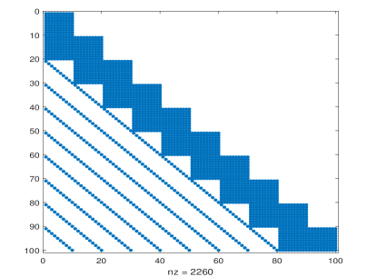
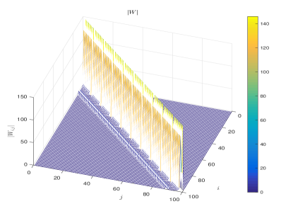
Fig. 1: The sparsity pattern (Left) and decay elements (Right) of matrix $W\in\mathbb{R}^{100\times 100}$, when $M=N=11$.

To approximate the coefficient matrix $W$ well, an example of the matrix $W$ is plotted in Fig. 1 corresponding to $h=\tau=\frac{1}{11}$. Fig. 1(a) shows the sparsity pattern of $W$. From Fig. 1(b), it is noticeable that the diagonal entries of $W$ decay quickly, i.e., the main information of $W$ clustered in the first two nonzero block diagonals. Inspired by this observation, a block bi-diagonal Toeplitz preconditioner $P_{W}$ is developed for the linear system (2.5b), which only preserves the first two nonzero block diagonals of $W$, more precisely,

$$P_{W}=\begin{bmatrix}A_{0}&\bm{0}&\bm{0}&\cdots&\bm{0}&\bm{0}\\ A_{1}&A_{0}&\bm{0}&\bm{0}&\cdots&\bm{0}\\ \bm{0}&A_{1}&A_{0}&\ddots&\ddots&\vdots\\ \vdots&\ddots&\ddots&\ddots&\ddots&\bm{0}\\ \bm{0}&\ddots&\ddots&\ddots&A_{0}&\bm{0}\\ \bm{0}&\bm{0}&\cdots&\cdots&A_{1}&A_{0}\end{bmatrix}.$$ (3.1)

Clearly $P_{W}$ is a block-Toeplitz matrix with Toeplitz-blocks, thus its memory requirement is of $\mathcal{O}(N)$.

Several properties of $\omega^{(\beta)}_{k}$ are reviewed in the following lemma, which is helpful to analyze the nonsingularity of $P_{W}$.

Lemma 3.1

([32, 33]) Suppose that $1<\beta<2$, then the coefficients $\omega_{k}^{(\beta)}$ satisfy

$$\begin{cases}\omega_{0}^{(\beta)}=\frac{\beta}{2}>0,~{}~{}\omega_{1}^{(\beta)}=\frac{2-\beta-\beta^{2}}{2}<0,~{}~{}\omega_{2}^{(\beta)}=\frac{\beta(\beta^{2}+\beta-4)}{4},\\ 1\geq\omega_{0}^{(\beta)}\geq\omega_{3}^{(\beta)}\geq\omega_{4}^{(\beta)}\geq\cdots\geq 0,~{}~{}\omega_{0}^{(\beta)}+\omega_{2}^{(\beta)}>0,\\ \sum\limits_{k=0}^{\infty}\omega_{k}^{(\beta)}=0,~{}~{}\sum\limits_{k=0}^{N}\omega_{k}^{(\beta)}<0,~{}~{}N\geq 2.\end{cases}$$

As seen from Lemma 3.1, we proceed to analyze the nonsingularity of $P_{W}$.

Theorem 3.1

$P_{W}$ given in (3.1) is nonsingular.

Proof. Since $P_{W}$ is a block lower bi-diagonal matrix, the proof of this theorem is equivalent to prove the nonsingularity of $A_{0}$.

Firstly, we show that all eigenvalues of matrix $H=\frac{K_{N}+K_{N}^{T}}{2}$ are strictly negative. From the definition of $K_{N}$ in (2.2), it has $H=\frac{e_{1}+e_{2}}{2}\left(G_{\beta}+G_{\beta}^{T}\right)$. Then according to the Gershgorin circle theorem [34], the $i$-th Gershgorin disc of $H$ is centered at $\left(e_{1}+e_{2}\right)\omega_{1}^{(\beta)}<0$ with radius

$$r_{i}^{\beta}=\frac{e_{1}+e_{2}}{2}\left(\sum\limits_{k=0,k\neq 1}^{i}\omega_{k}^{(\beta)}+\sum\limits_{k=0,k\neq 1}^{N-i}\omega_{k}^{(\beta)}\right)\leq\left(e_{1}+e_{2}\right)\sum\limits_{k=0,k\neq 1}^{N}\omega_{k}^{(\beta)}<-\left(e_{1}+e_{2}\right)\omega_{1}^{(\beta)}~{}(1\leq i\leq N-1),$$

in which Lemma 3.1 is adopted. Thus the real parts of all eigenvalues of $A_{0}$ are strictly positive. The proof of Theorem 3.1 is completed. $\Box$

Theorem 3.1 also implies that the matrices $A$ and $W$ are invertible. Now, the eigenvalues of the preconditioned matrix $P_{W}^{-1}W$ can be studied.

Theorem 3.2

The eigenvalues of the preconditioned matrix $P_{W}^{-1}W$ are all equal to $1$.

Proof. It is known that the product of two block lower triangular matrices also is a block lower triangular matrix. After simple calculations, it notes that

$$P_{W}^{-1}W=\begin{bmatrix}I&\bm{0}&\cdots&\cdots&\bm{0}\\ \bm{0}&I&\ddots&\ddots&\vdots\\ J_{2}&\ddots&\ddots&\ddots&\vdots\\ \vdots&\ddots&\ddots&\ddots&\bm{0}\\ J_{M-2}&J_{M-3}&\cdots&\cdots&I\end{bmatrix}$$

is a block lower triangular matrix, where $J_{2}=A_{0}^{-1}A_{2}$, $J_{k}=A_{0}^{-1}\left(A_{k}-A_{1}J_{k-1}\right)~{}(3\leq k\leq M-2)$. From the above equality, the main diagonal elements of $P_{W}^{-1}W$ are $1$, which completes the proof. $\Box$

Remark 1

The preconditioned Krylov subspace methods require us to compute $P_{W}^{-1}\bm{v}$, where $\bm{v}$ is a vector. In this work, the Thomas method is employed to compute such matrix-vector multiplications. Hence, only $A_{0}^{-1}\bm{v}$ is needed to compute. In practical computation, the Toeplitz inversion formula [35] combined with Krylov subspace methods is used to calculate $A_{0}^{-1}\bm{v}$, and this will be discussed in Section 3.2.

For the sake of clarity, the Thomas method for calculating $P_{W}^{-1}\bm{v}$ is given as below.

Algorithm 1 Compute $\bm{z}=P_{W}^{-1}\bm{v}$

1:  Reshape $\bm{v}$ into an $(N-1)\times M$ matrix $\check{V}$

2:  Compute $\bm{\hat{b}}_{1}=A_{0}^{-1}\check{V}(:,1)$ via Algorithm 2 in Section 3.2

3:  for $k=2,\cdots,M$ do

4:     $\bm{\varphi}=\check{V}(:,k)-A_{1}\hat{\bm{b}}_{k-1}$

5:     $\bm{\hat{b}}_{k}=A_{0}^{-1}\bm{\varphi}$ via Algorithm 2 in Section 3.2

6:  end for

7:  Stack $\bm{\hat{b}}_{k}~{}(k=1,\cdots,M)$ in a vector $\bm{z}$

In line 4 of Algorithm 1, the matrix-vector multiplications can be done via FFTs in $\mathcal{O}(N\log N)$ operations [28, 29]. As for the storage requirement, $\bm{v}$, $\bm{\hat{b}}_{k}$, $\bm{\varphi}$, the first column and first row of $A_{1}$ must be stored. Thus only $\mathcal{O}(MN)$ memory is needed in Algorithm 1.

3.2 A skew-circulant preconditioner

According to the Toeplitz inversion formula in [35], two Toeplitz systems

$$\begin{cases}A_{0}\bm{\xi}=\bm{q}_{1},\\ A_{0}\bm{\eta}=\bm{q}_{N-1}\end{cases}$$ (3.2)

require to be solved, where $\bm{\xi}=[\xi_{1},\cdots,\xi_{N-1}]^{T}$, $\bm{\eta}=[\eta_{1},\cdots,\eta_{N-1}]^{T}$, $\bm{q}_{1}$ and $\bm{q}_{N-1}$ are the first and last columns of the identity matrix of order $(N-1)$, respectively. As mentioned in Remark 1, Krylov subspace methods are chosen to solve (3.2). However, when $A_{0}$ is ill-conditioned, Krylov subspace methods converge very slowly. To remedy such difficulties, in this subsection, a new skew-circulant preconditioner $P_{sk}$ is designed and the spectrum of $P_{sk}^{-1}A_{0}$ is discussed. The expression of our skew-circulant $P_{sk}$ is given as follows

$$P_{sk}=h^{\beta}c_{0}^{(\alpha,\sigma)}I-\sigma sk(K_{N}),$$ (3.3)

where $sk(K_{N})=e_{1}sk(G_{\beta})+e_{2}sk(G_{\beta})^{T}$ with

$$sk(G_{\beta})=\begin{bmatrix}\omega_{1}^{(\beta)}&\omega_{0}^{(\beta)}&-\omega_{N-2}^{(\beta)}&\cdots&-\omega_{2}^{(\beta)}\\ \omega_{2}^{(\beta)}&\omega_{1}^{(\beta)}&\omega_{0}^{(\beta)}&\ddots&\vdots\\ \vdots&\ddots&\ddots&\ddots&-\omega_{N-2}^{(\beta)}\\ \omega_{N-2}^{(\beta)}&\ddots&\ddots&\ddots&\omega_{0}^{(\beta)}\\ -\omega_{0}^{(\beta)}&\omega_{N-2}^{(\beta)}&\cdots&\omega_{2}^{(\beta)}&\omega_{1}^{(\beta)}\end{bmatrix}\in\mathbb{R}^{(N-1)\times(N-1)}.$$

Similar to the proof of Theorem 3.1, the following theorem provide an essential property of $P_{sk}$ in (3.3).

Theorem 3.3

The matrix $P_{sk}$ given in (3.3) is invertible.

Proof. Firstly, we prove that all eigenvalues of matrix $\hat{H}=-\frac{sk(K_{N})+sk(K_{N})^{T}}{2}$ are strictly positive. Based on the definition of $sk(G_{\beta})$ and the Gershgorin circle theorem [34], all the Gershgorin disc of the matrix $\hat{H}$ are centered at $-\left(e_{1}+e_{2}\right)\omega_{1}^{(\beta)}>0$ with radius

$$r=\frac{e_{1}+e_{2}}{2}\left[2\left(\omega_{0}^{(\beta)}+\omega_{2}^{(\beta)}\right)+\sum\limits_{k=3}^{N-2}\left|\omega_{k}^{(\beta)}-\omega_{N+1-k}^{(\beta)}\right|\right]\leq\left(e_{1}+e_{2}\right)\sum\limits_{k=0,k\neq 1}^{N}\omega_{k}^{(\beta)}\leq-\left(e_{1}+e_{2}\right)\omega_{1}^{(\beta)}.$$

Thus, the real parts of all eigenvalues of $P_{sk}$ are strictly positive. Then the targeted result follows. $\Box$

An $n\times n$ skew-circulant matrix $\mathcal{C}$ has the spectral decomposition [28, 29]:

$$\mathcal{C}=\Omega^{*}F^{*}\Lambda F\Omega,$$

here $\Omega=\textrm{diag}\left[1,(-1)^{-1/n},\cdots,(-1)^{-(n-1)/n}\right]$, $F$ is the discrete Fourier matrix, $F^{*}$ represents the conjugate transpose of $F$, and $\Lambda$ is a diagonal matrix containing all eigenvalues of $\mathcal{C}$. Let $sk(G_{\beta})=\Omega^{*}F^{*}\Lambda_{s}F\Omega$, then $sk(G_{\beta})^{T}=\Omega^{*}F^{*}\bar{\Lambda}_{s}F\Omega$ and $P_{sk}=\Omega^{*}F^{*}\Lambda F\Omega$, where $\Lambda=h^{\beta}c_{0}^{(\alpha,\sigma)}I-\sigma\left(e_{1}\Lambda_{s}+e_{2}\bar{\Lambda}_{s}\right)$ and $\bar{\Lambda}_{s}$ is the complex conjugate of $\Lambda_{s}$. With the help of the decomposition of $P_{sk}$, the following result is obtained immediately.

Lemma 3.2

Suppose $0<\hat{v}<h^{\beta}c_{0}^{(\alpha,\sigma)}$, then $\parallel P_{sk}^{-1}\parallel_{2}\leq\frac{1}{\hat{v}}$.

Proof. By Theorem 3.3, we obtain $Re([\Lambda_{s}]_{k,k})<0$, where $Re([\Lambda_{s}]_{k,k})$ means the real part of $[\Lambda_{s}]_{k,k}$. Then

$$\left|[\Lambda]_{k,k}\right|\geq Re([\Lambda]_{k,k})=h^{\beta}c_{0}^{(\alpha,\sigma)}-\sigma\left(e_{1}Re([\Lambda_{s}]_{k,k})+e_{2}Re([\bar{\Lambda}_{s}]_{k,k})\right)\geq\hat{v},~{}k=1,2,\cdots,N-1.$$

Therefore

$$\parallel P_{sk}^{-1}\parallel_{2}=\frac{1}{\min\limits_{1\leq k\leq N-1}\left|[\Lambda]_{k,k}\right|}\leq\frac{1}{\hat{v}}.$$

$\Box$

To analyze the spectrum of $P_{sk}^{-1}A_{0}$, we first prove that the generating function of the Toeplitz matrix $K_{N}$ is in the Wiener class [29].

Lemma 3.3

The generating function of the sequence $\left\{K_{N}\right\}_{N=2}^{\infty}$ is in the Wiener class.

Proof. For the Toeplitz matrix $K_{N}$ in (2.2), its generating function is

$$p(\theta)=\sum\limits_{k=-\infty}^{\infty}\ell_{k}e^{\bm{i}k\theta}=\sum\limits_{k=-1}^{\infty}\omega_{k+1}^{(\beta)}\left(e_{1}e^{\bm{i}k\theta}+e_{2}e^{-\bm{i}k\theta}\right),$$

where $\bm{i}=\sqrt{-1}$ and $\theta\in[-\pi,\pi]$. By the properties of $\omega_{k}^{(\beta)}$, it yields

$$\sum\limits_{k=-\infty}^{\infty}\left|\ell_{k}\right|\leq\left(e_{1}+e_{2}\right)\sum\limits_{k=-1}^{\infty}\left|\omega_{k+1}^{(\beta)}\right|=\left(e_{1}+e_{2}\right)\left(-2\omega_{1}^{(\beta)}+\left|\omega_{2}^{(\beta)}\right|-\omega_{2}^{(\beta)}\right)<\infty.$$

Thus, the generating function $p(\theta)$ is in the Wiener class. $\Box$

According to Lemma 3.3, the following result is true.

Lemma 3.4

Let $p(\theta)$ be the generating function of $K_{N}$. Then for any $\varepsilon>0$, there exists an $N^{\prime}>0$, such that for all $N>N^{\prime}+1$, $A_{0}-P_{sk}=\tilde{U}+\tilde{V}$, where $rank(\tilde{U})<2N^{\prime}$ and $\parallel\tilde{V}\parallel_{2}\leq\varepsilon$.

Proof. Define $D_{sk}=A_{0}-P_{sk}=\sigma\left(sk(K_{N})-K_{N}\right)$. It can be checked that $D_{sk}$ is a Toeplitz matrix, and its first column and first row are respectively

$$\begin{split}&-\sigma[0,0,e_{2}\omega_{N-2}^{(\beta)},\cdots,e_{2}\omega_{3}^{(\beta)},e_{1}(\omega_{0}^{(\beta)}+\omega_{N-2}^{(\beta)})+e_{2}\omega_{2}^{(\beta)}]^{T},\\ &-\sigma[0,0,e_{1}\omega_{N-2}^{(\beta)},\cdots,e_{1}\omega_{3}^{(\beta)},e_{1}\omega_{2}^{(\beta)}+e_{2}(\omega_{0}^{(\beta)}+\omega_{N-2}^{(\beta)})].\end{split}$$

Using Lemma 3.3, we know that $p(\theta)$ is in the Wiener class. Then for any $\varepsilon>0$, there exists an $N^{\prime}>0$ such that $\sum\limits_{k=N^{\prime}+1}^{\infty}\left|\ell_{k}\right|=e_{2}\sum\limits_{k=N^{\prime}+1}^{\infty}\left|\omega_{k+1}^{(\beta)}\right|\leq\frac{e_{2}\varepsilon}{\sigma(e_{1}+e_{2})}$. Let $\tilde{V}$ be the $(N-1)$-by-$(N-1)$ matrix obtained from $D_{sk}$ by copying the $(N-1-N^{\prime})$-by-$(N-1-N^{\prime})$ leading principal submatrix of $D_{sk}$. Hence the leading $(N-1-N^{\prime})\times(N-1-N^{\prime})$ block of $\tilde{V}$ is a Toeplitz matrix. Thus

$$\begin{split}\parallel\tilde{V}\parallel_{1}&=\sigma\max\left\{\sum\limits_{k=N^{\prime}+1}^{N-3}\left|\ell_{k}\right|,\sum\limits_{k=N^{\prime}+1}^{N-3}\left|\ell_{-k}\right|,\max\limits_{3\leq j\leq N-3-N^{\prime}}\left(\sum\limits_{k=N^{\prime}+j}^{N-3}\left|\ell_{k}\right|+\sum\limits_{k=N-j}^{N-3}\left|\ell_{-k}\right|\right)\right\}\\ &\leq\sigma(e_{1}+e_{2})\sum\limits_{k=N^{\prime}+1}^{\infty}\left|\omega_{k+1}^{(\beta)}\right|\leq\varepsilon.\end{split}$$

Similarly, $\parallel\tilde{V}\parallel_{\infty}\leq\varepsilon$. Thus $\parallel\tilde{V}\parallel_{2}\leq\left(\parallel\tilde{V}\parallel_{1}\cdot\parallel\tilde{V}\parallel_{\infty}\right)^{1/2}\leq\varepsilon$.

Let $\tilde{U}=D_{sk}-\tilde{V}$. It is obvious that $\tilde{U}$ is an $(N-1)\times(N-1)$ matrix obtained from $D_{sk}$ by replacing the $(N-1-N^{\prime})\times(N-1-N^{\prime})$ leading principal submatrix of $D_{sk}$ by the zero matrix. Hence $rank(\tilde{U})\leq 2N^{\prime}$. $\Box$

Combining Lemmas 3.2 and 3.4, the spectrum of $P_{sk}^{-1}A_{0}-I$ is discussed.

Theorem 3.4

Suppose $0<\hat{v}<h^{\beta}c_{0}^{(\alpha,\sigma)}$. Then for any $\varepsilon>0$, there exists an $N^{\prime}>0$, such that for all $N-1>N^{\prime}$, $P_{sk}^{-1}A_{0}-I=U+V$, where $rank(U)<2N^{\prime}$ and $\parallel V\parallel_{2}\leq\frac{\varepsilon}{\hat{v}}$.

Proof. According to Lemma 3.4, for any $\varepsilon>0$, there exists an $N^{\prime}>0$, such that for all $N-1>N^{\prime}$,

$$P_{sk}^{-1}A_{0}-I=P_{sk}^{-1}\left(A_{0}-P_{sk}\right)=U+V,$$

where $U=P_{sk}^{-1}\tilde{U}$ and $V=P_{sk}^{-1}\tilde{V}$. Applying Lemma 3.2, it yields

$$\parallel V\parallel_{2}=\parallel P_{sk}^{-1}\tilde{V}\parallel_{2}\leq\parallel P_{sk}^{-1}\parallel_{2}\parallel\tilde{V}\parallel_{2}\leq\frac{\varepsilon}{\hat{v}}.$$

On the other hand, $rank(U)=rank(P_{sk}^{-1}\tilde{U})<2N^{\prime}$. $\Box$

Remark 2

Since the matrix $A$ is slightly different to $A_{0}$, the $P_{sk}$ in (3.3) still works for solving (2.5a). Hence, in this work, $P_{sk}$ is also applied to solve (2.5a).

For convenience, our strategy in this subsection is concluded in the following algorithm.

Algorithm 2 Compute $\bm{\tilde{z}}=A_{0}^{-1}\bm{v}$

1:  Solve $A_{0}\bm{\xi}=\bm{q}_{1}$ via FGMRES/PBiCGSTAB with $P_{sk}$ Solve $A_{0}\bm{\eta}=\bm{q}_{N-1}$ via FGMRES/PBiCGSTAB with $P_{sk}$

2:  $\bm{s}_{1}=[\eta_{N-1},-\eta_{1},\cdots,-\eta_{N-2}]^{T}$, $\bm{s}_{2}=[\eta_{N-1},\eta_{1},\cdots,\eta_{N-2}]^{T}$

3:  $\Lambda^{(1)}=\textrm{diag}(F\bm{\xi})$,  $\Lambda^{(2)}=\textrm{diag}(\Omega^{*}F\bm{s}_{1})$, $\Lambda^{(3)}=\textrm{diag}(F\bm{s}_{2})$, $\Lambda^{(4)}=\textrm{diag}(\Omega^{*}F\bm{\xi})$

4:  $\bm{\tilde{v}}=F\Omega\bm{v}$

5:  $\bm{z}_{1}=\Omega^{*}F^{*}\Lambda^{(2)}\bm{\tilde{v}}$,  $\bm{z}_{2}=\Omega^{*}F^{*}\Lambda^{(4)}\bm{\tilde{v}}$, $\bm{z}_{3}=\Lambda^{(1)}F\bm{z}_{1}$,    $\bm{z}_{4}=\Lambda^{(3)}F\bm{z}_{2}$

6:  $\bm{\tilde{z}}=\frac{1}{2\xi_{1}}F^{*}(\bm{z}_{3}+\bm{z}_{4})$

In this algorithm, ten fast Fourier transforms are needed. Thus, the complexity and storage requirement are $\mathcal{O}(N\log N)$ and $\mathcal{O}(N)$, respectively.

4 Numerical experiments

In this section, one example is reported to show the performance of the proposed preconditioners in Section 3. In order to illustrate the efficiency of $P_{sk}$, the Strang’s circulant preconditioner [28, 29] is also tested, which can be written as

$$P_{s}=h^{\beta}c_{0}^{(\alpha,\sigma)}I-\sigma s(K_{N}),$$

where $s(K_{N})=e_{1}s(G_{\beta})+e_{2}s(G_{\beta})^{T}$. More precisely, the first columns of circulant matrices $s(G_{\beta})$ and $s(G_{\beta})^{T}$ are $\left[\omega_{1}^{(\beta)},\cdots,\omega_{\lfloor N/2\rfloor}^{(\beta)},0,\cdots,0,\omega_{0}^{(\beta)}\right]^{T}$ and $\left[\omega_{1}^{(\beta)},\omega_{0}^{(\beta)},0,\cdots,0,\omega_{\lfloor N/2\rfloor}^{(\beta)},\cdots,\omega_{2}^{(\beta)}\right]^{T}$, respectively.

The PBiCGSTAB and FGMRES methods for solving (2.5) terminate if the relative residual error satisfies $\frac{\|\bm{r}^{(k)}\|_{2}}{\|\bm{r}^{(0)}\|_{2}}<10^{-8}$ or the iteration number is more than $1000$, where $\bm{r}^{(k)}$ denotes residual vector in the $k$-th iteration, and the initial guess is chosen as the zero vector. Since the $P_{W}$ as a preconditioner for solving (2.5), it is not necessary to compute the $P^{-1}_{W}\bm{v}$ accurately. Hence the stop criterion of PBiCGSTAB or FGMRES methods in Algorithm 2 is $\frac{\|\bm{r}^{(k)}\|_{2}}{\|\bm{r}^{(0)}\|_{2}}<10^{-3}$, and the initial guess is also chosen as the zero vector. All of the symbols shown below will appear in later.

All experiments are carried out via MATLAB 2017a on a Windows 10 (64 bit) PC with the configuration: Intel(R) Core(TM) i7-7700T CPU 2.90 GHz and 8 GB RAM.

Symbol	Explanation
BS	The MATLAB’s backslash method to solve (2.5)
BFSM	The BFS method to solve (2.5)
SK2-PBiCGSTAB	The PBiCGSTAB method with the preconditioners $P_{W}$ and $P_{sk}$ to solve (2.5)
SK2-FGMRES	The FGMRES method with the preconditioners $P_{W}$ and $P_{sk}$ to solve (2.5)
S2-PBiCGSTAB	The PBiCGSTAB method with the preconditioners $P_{W}$ and $P_{s}$ to solve (2.5)
S2-FGMRES	The FGMRES method with the preconditioners $P_{W}$ and $P_{s}$ to solve (2.5)
$\mathrm{Iter1}$	The number of iterations required for solving (2.5a)
$\mathrm{Iter2}$	The number of iterations required for solving (2.5b)
$\mathrm{Iter3}$	The number of iterations required for solving (3.2)
$\mathrm{Iter}$	$\mathrm{Iter1}+\mathrm{Iter2}$
Time	Total CPU time in seconds for solving the whole BLTT system (2.5)
†	Out of memory

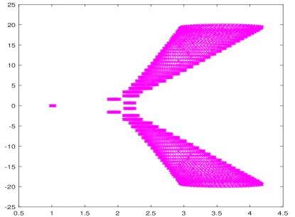
(a) Eigenvalues of $W$

(b) Eigenvalues of $P_{W}^{-1}W$

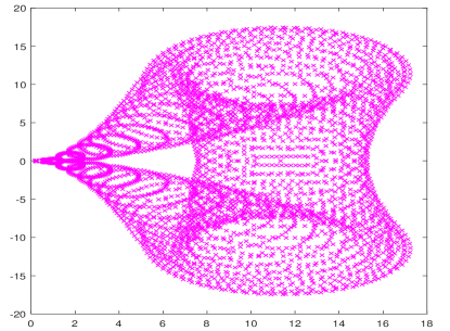
(c) Eigenvalues of $W$

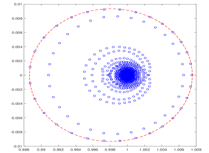
(d) Eigenvalues of $P_{W}^{-1}W$

Fig. 2: Spectra of $W$ and $P_{W}^{-1}W$, when $M=N=2^{6}$ in Example 1. Top row: $(\alpha,\beta)=(0.1,1.1)$; Bottom row: $(\alpha,\beta)=(0.7,1.4)$.

Example 1. Considering Eq. (1.1) with diffusion coefficients $e_{1}=20$, $e_{2}=0.02$, the source term

$$\begin{split}f(x,t)=&2t^{1-\alpha}E_{1,2-\alpha}(2t)x^{2}(1-x)^{2}-e^{2t}\Bigg{\{}\frac{\Gamma(3)}{\Gamma(3-\beta)}\left[e_{1}x^{2-\beta}+e_{2}(1-x)^{2-\beta}\right]\\ &-\frac{2\Gamma(4)}{\Gamma(4-\beta)}\left[e_{1}x^{3-\beta}+e_{2}(1-x)^{3-\beta}\right]+\frac{\Gamma(5)}{\Gamma(5-\beta)}\left[e_{1}x^{4-\beta}+e_{2}(1-x)^{4-\beta}\right]\Bigg{\}},\end{split}$$

in which $E_{\mu,\nu}(z)$ is the Mittag-Leffler function [5] with two parameters defined by

$$E_{\mu,\nu}(z)=\sum_{k=0}^{\infty}\frac{z^{k}}{\Gamma(\mu k+\nu)}.$$

The exact solution of the TSFDE problem (1.1) is $u(x,t)=e^{2t}x^{2}(1-x)^{2}$.

(a) Eigenvalues of $A_{0}$

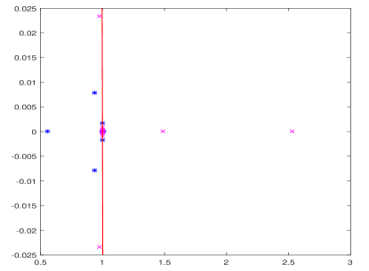
(b) Eigenvalues of $P_{sk}^{-1}A_{0}$ ( $*$) and $P_{s}^{-1}A_{0}$ ( $\times$)

(c) Eigenvalues of $A_{0}$

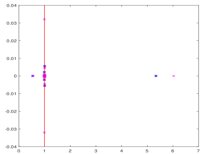
(d) Eigenvalues of $P_{sk}^{-1}A_{0}$ ( $*$) and $P_{s}^{-1}A_{0}$ ( $\times$)

Fig. 3: Spectra of $A_{0}$, $P_{s}^{-1}A_{0}$ and $P_{s}^{-1}A_{0}$, when $M=N=2^{8}$ in Example 1. Top row: $(\alpha,\beta)=(0.1,1.1)$; Bottom row: $(\alpha,\beta)=(0.7,1.4)$.

Table 1: Results of different methods when $M=N$ for Example 1.

		BS	BFSM	SK2-PBiCGSTAB		S2-PBiCGSTAB		SK2-FGMRES		S2-FGMRES
($\alpha$, $\beta$)	$N$	$\mathrm{Time}$	$\mathrm{Time}$	($\mathrm{Iter}$, $\mathrm{Iter3}$)	$\mathrm{Time}$	($\mathrm{Iter}$, $\mathrm{Iter3}$)	$\mathrm{Time}$	($\mathrm{Iter}$, $\mathrm{Iter3}$)	$\mathrm{Time}$	($\mathrm{Iter}$, $\mathrm{Iter3}$)	$\mathrm{Time}$
(0.1, 1.1)	64	0.213	0.007	(4+2, 5)	0.014	(5+2, 5)	0.015	(6+5, 5)	0.020	(6+5, 6)	0.021
	128	3.469	0.044	(4+2, 5)	0.056	(5+2, 5)	0.057	(6+5, 5)	0.077	(6+6, 5)	0.092
	256	237.015	0.234	(5+2, 5)	0.142	(5+2, 5)	0.144	(6+6, 5)	0.234	(6+7, 5)	0.273
	512	†	1.839	(5+2, 5)	0.995	(5+2, 5)	0.998	(6+7, 5)	1.912	(6+8, 5)	2.185
	1024	†	19.839	(5+2, 5)	2.635	(5+2, 6)	2.672	(6+9, 5)	6.672	(6+10, 5)	7.480
(0.4, 1.7)	64	0.185	0.009	(4+2, 5)	0.014	(6+2, 6)	0.015	(6+5, 7)	0.021	(7+5, 6)	0.022
	128	2.993	0.043	(4+2, 5)	0.057	(6+2, 5)	0.058	(6+6, 6)	0.090	(7+5, 6)	0.078
	256	232.214	0.235	(6+2, 5)	0.140	(6+2, 5)	0.141	(6+7, 6)	0.268	(7+6, 5)	0.233
	512	†	1.840	(6+3, 5)	1.486	(6+3, 5)	1.485	(6+7, 5)	1.906	(7+6, 5)	1.664
	1024	†	19.838	(6+3, 5)	3.887	(6+3, 5)	3.878	(6+8, 5)	5.983	(7+7, 5)	5.248
(0.7, 1.4)	64	0.183	0.009	(4+3, 5)	0.020	(5+3, 5)	0.020	(6+6, 7)	0.024	(6+6, 8)	0.025
	128	2.969	0.040	(5+3, 5)	0.081	(5+3, 5)	0.083	(6+7, 6)	0.104	(7+8, 6)	0.119
	256	237.030	0.238	(5+4, 5)	0.279	(5+4, 5)	0.279	(6+8, 6)	0.300	(7+9, 6)	0.342
	512	†	1.842	(5+4, 5)	1.975	(5+4, 5)	1.988	(6+10, 5)	2.688	(7+11, 6)	2.971
	1024	†	19.847	(5+5, 5)	6.429	(5+5, 5)	6.526	(6+11, 5)	8.174	(7+14, 5)	10.540
(0.9, 1.9)	64	0.176	0.009	(4+2, 5)	0.015	(6+2, 5)	0.016	(5+5, 5)	0.200	(6+5, 5)	0.021
	128	2.950	0.043	(6+3, 5)	0.081	(6+3, 5)	0.082	(6+6, 5)	0.091	(6+6, 5)	0.092
	256	233.143	0.209	(6+3, 5)	0.209	(6+3, 5)	0.214	(6+7, 5)	0.267	(6+7, 5)	0.271
	512	†	1.837	(6+4, 5)	1.968	(6+4, 5)	1.986	(6+8, 5)	2.164	(6+8, 5)	2.182
	1024	†	19.853	(6+4, 5)	5.211	(6+4, 5)	5.276	(6+10, 5)	7.505	(6+10, 5)	7.447

Table 2: Results of different methods when $M=257$ for Example 1.

		BS	BFSM	SK2-PBiCGSTAB		S2-PBiCGSTAB		SK2-FGMRES		S2-FGMRES
($\alpha$, $\beta$)	$N$	$\mathrm{Time}$	$\mathrm{Time}$	($\mathrm{Iter}$, $\mathrm{Iter3}$)	$\mathrm{Time}$	($\mathrm{Iter}$, $\mathrm{Iter3}$)	$\mathrm{Time}$	($\mathrm{Iter}$, $\mathrm{Iter3}$)	$\mathrm{Time}$	($\mathrm{Iter}$, $\mathrm{Iter3}$)	$\mathrm{Time}$
(0.1, 1.1)	65	3.198	0.077	(4+2, 5)	0.053	(5+2, 5)	0.055	(6+5, 5)	0.075	(6+5, 6)	0.072
	129	13.545	0.115	(4+2, 5)	0.079	(5+2, 5)	0.079	(6+5, 5)	0.111	(6+6, 5)	0.138
	257	277.409	0.209	(5+2, 5)	0.138	(5+2, 5)	0.138	(6+6, 5)	0.236	(6+7, 5)	0.269
	513	†	0.819	(5+2, 5)	0.236	(5+2, 5)	0.237	(6+7, 5)	0.462	(6+8, 5)	0.527
	1025	†	4.613	(5+2, 5)	0.405	(5+2, 6)	0.418	(6+9, 5)	1.078	(6+10, 5)	1.205
(0.4, 1.7)	65	3.116	0.072	(4+2, 5)	0.050	(6+2, 6)	0.059	(6+5, 7)	0.066	(7+6, 6)	0.077
	129	13.397	0.119	(4+2, 5)	0.080	(6+2, 5)	0.084	(6+6, 6)	0.131	(7+6, 6)	0.137
	257	263.419	0.210	(6+2, 5)	0.139	(6+2, 5)	0.139	(6+7, 6)	0.271	(7+6, 5)	0.238
	513	†	0.816	(6+2, 5)	0.233	(6+2, 5)	0.232	(6+7, 5)	0.474	(7+6, 5)	0.421
	1025	†	4.613	(6+2, 5)	0.410	(6+3, 5)	0.615	(6+7, 5)	0.840	(7+6, 5)	0.760
(0.7, 1.4)	65	3.056	0.073	(4+4, 5)	0.093	(5+4, 5)	0.100	(6+8, 6)	0.101	(6+8, 7)	0.109
	129	13.421	0.115	(5+4, 5)	0.155	(5+4, 5)	0.165	(6+8, 6)	0.172	(7+9, 6)	0.199
	257	251.611	0.214	(5+4, 5)	0.269	(5+4, 5)	0.277	(6+8, 6)	0.298	(7+9, 6)	0.334
	513	†	0.833	(5+4, 5)	0.450	(5+4, 5)	0.457	(6+9, 6)	0.593	(7+10, 6)	0.658
	1025	†	4.397	(5+4, 5)	0.792	(5+4, 5)	0.793	(7+10, 5)	1.203	(7+11, 6)	1.332
(0.9, 1.9)	65	3.057	0.070	(4+3, 5)	0.074	(6+3, 5)	0.071	(6+7, 5)	0.088	(6+7, 5)	0.102
	129	13.393	0.118	(4+3, 5)	0.116	(6+3, 5)	0.124	(6+7, 5)	0.152	(6+7, 5)	0.160
	257	257.493	0.211	(6+3, 5)	0.201	(6+3, 5)	0.213	(6+7, 5)	0.263	(6+7, 5)	0.274
	513	†	0.828	(6+3, 5)	0.340	(6+3, 5)	0.365	(6+7, 5)	0.465	(6+7, 5)	0.482
	1025	†	4.625	(6+3, 5)	0.587	(6+3, 5)	0.613	(6+7, 5)	0.854	(6+7, 5)	0.860

Table 3: Results of different methods when $N=257$ for Example 1.

		BS	BFSM	SK2-PBiCGSTAB		S2-PBiCGSTAB		SK2-FGMRES		S2-FGMRES
($\alpha$, $\beta$)	$M$	$\mathrm{Time}$	$\mathrm{Time}$	($\mathrm{Iter}$, $\mathrm{Iter3}$)	$\mathrm{Time}$	($\mathrm{Iter}$, $\mathrm{Iter3}$)	$\mathrm{Time}$	($\mathrm{Iter}$, $\mathrm{Iter3}$)	$\mathrm{Time}$	($\mathrm{Iter}$, $\mathrm{Iter3}$)	$\mathrm{Time}$
(0.1, 1.1)	65	4.065	0.048	(5+2, 5)	0.035	(5+2, 5)	0.037	(6+6, 5)	0.059	(6+7, 5)	0.067
	129	23.278	0.091	(5+2, 5)	0.063	(5+2, 5)	0.070	(6+6, 5)	0.113	(6+7, 5)	0.135
	257	277.409	0.209	(5+2, 5)	0.138	(5+2, 5)	0.138	(6+6, 5)	0.236	(6+7, 5)	0.269
	513	†	0.569	(5+2, 5)	0.257	(5+2, 5)	0.266	(6+6, 5)	0.463	(6+7, 5)	0.550
	1025	†	1.702	(5+2, 5)	0.530	(5+2, 5)	0.542	(6+6, 5)	0.958	(6+7, 5)	1.095
(0.4, 1.7)	65	4.057	0.047	(6+2, 5)	0.036	(6+2, 5)	0.039	(6+7, 6)	0.069	(7+6, 5)	0.067
	129	22.929	0.088	(5+2, 5)	0.068	(6+2, 5)	0.071	(6+7, 6)	0.125	(7+6, 5)	0.118
	257	263.419	0.210	(6+2, 5)	0.139	(6+2, 5)	0.139	(6+7, 6)	0.271	(7+6, 5)	0.238
	513	†	0.585	(6+3, 5)	0.390	(6+3, 5)	0.396	(6+7, 6)	0.534	(7+6, 5)	0.476
	1025	†	1.854	(6+3, 5)	0.782	(6+3, 5)	0.810	(6+7, 6)	1.101	(7+6, 5)	0.968
(0.7, 1.4)	65	4.069	0.048	(5+3, 5)	0.051	(5+3, 5)	0.550	(6+9, 6)	0.088	(7+8, 6)	0.079
	129	23.217	0.090	(5+3, 5)	0.099	(5+3, 5)	0.106	(6+8, 6)	0.146	(7+8, 6)	0.151
	257	251.611	0.214	(5+4, 5)	0.269	(5+4, 5)	0.277	(6+8, 6)	0.298	(7+9, 6)	0.334
	513	†	0.578	(4+4, 5)	0.521	(5+4, 5)	0.542	(6+9, 6)	0.680	(7+10, 6)	0.776
	1025	†	1.763	(4+5, 5)	1.301	(5+5, 5)	1.318	(6+11, 5)	1.680	(7+12, 6)	1.829
(0.9, 1.9)	65	4.081	0.043	(6+2, 5)	0.036	(6+2, 5)	0.039	(6+5, 5)	0.049	(6+5, 5)	0.053
	129	23.093	0.095	(6+3, 5)	0.098	(6+3, 5)	0.106	(6+6, 5)	0.112	(6+6, 5)	0.119
	257	257.493	0.211	(6+3, 5)	0.201	(6+3, 5)	0.213	(6+7, 5)	0.263	(6+7, 5)	0.274
	513	†	0.552	(6+4, 5)	0.513	(6+4, 5)	0.539	(6+8, 5)	0.612	(6+8, 5)	0.642
	1025	†	1.725	(4+4, 5)	1.033	(6+4, 5)	1.082	(6+10, 5)	1.528	(6+10, 5)	1.567

Table 4: Comparison results of SK2-PBiCGSTAB method and Huang-Lei’s method for Example 1, where $M=257$.

		Huang-Lei’s method			SK2-PBiCGSTAB
($\alpha$, $\beta$)	$N$	$\mathrm{Time}$	$\mathrm{Error1}$	$\mathrm{Error2}$	$\mathrm{Time}$	$\mathrm{Error1}$	$\mathrm{Error2}$
(0.1, 1.1)	65	0.058	8.3526E-04	5.9916E-04	0.053	8.3526E-04	5.9916E-04
	129	0.065	2.1165E-04	1.5173E-04	0.079	2.1165E-04	1.5173E-04
	257	0.078	5.2851E-05	3.7902E-05	0.138	5.2852E-05	3.7903E-05
	513	0.116	1.2783E-05	9.2066E-06	0.236	1.2778E-05	9.2035E-06
	1025	0.233	2.7253E-06	2.0070E-06	0.405	2.7131E-06	1.9997E-06
(0.4, 1.7)	65	0.055	5.4781E-04	3.8003E-04	0.050	5.4781E-04	3.8003E-04
	129	0.063	1.3690E-04	9.5128E-05	0.080	1.3689E-04	9.5126E-05
	257	0.076	3.2744E-05	2.2885E-05	0.139	3.2743E-05	2.2884E-05
	513	0.115	6.6208E-06	4.7452E-06	0.233	6.6207E-06	4.7454E-06
	1025	0.224	1.5886E-06	4.9796E-07	0.410	1.5886E-06	4.9764E-07
(0.7, 1.4)	65	0.053	7.0888E-04	4.9767E-04	0.093	7.0888E-04	4.9767E-04
	129	0.064	1.7789E-04	1.2502E-04	0.155	1.7790E-04	1.2502E-04
	257	0.078	4.3826E-05	3.0074E-05	0.269	4.3825E-05	3.0076E-05
	513	0.120	1.1377E-05	6.1321E-06	0.450	1.1376E-05	6.1350E-06
	1025	0.220	2.9060E-06	5.7145E-07	0.792	2.9113E-06	5.4756E-07
(0.9, 1.9)	65	0.053	4.4937E-04	3.1623E-04	0.074	4.4937E-04	3.1623E-04
	129	0.064	1.1041E-04	7.7685E-05	0.116	1.1043E-04	7.7700E-05
	257	0.092	2.5058E-05	1.7763E-05	0.201	2.5028E-05	1.7741E-05
	513	0.126	3.8914E-06	2.8666E-06	0.340	3.8553E-06	2.8317E-06
	1025	0.220	1.7111E-06	1.0294E-06	0.587	1.7104E-06	1.0289E-06

Table 5: The condition numbers of $W$, $P_{W}^{-1}W$, $A_{0}$, $P_{s}^{-1}A_{0}$ and $P_{sk}^{-1}A_{0}$ in Example 1.

($\alpha$, $\beta$)	($N$, $M$)	$W$	$P_{W}^{-1}W$	$A_{0}$	$P_{s}^{-1}A_{0}$	$P_{sk}^{-1}A_{0}$
(0.1, 1.1)	(32, 32)	27.98	1.01	25.28	99.15	14.16
	(64, 32)	57.43	1.01	51.90	212.95	27.82
	(128, 32)	120.74	1.01	109.09	457.09	57.03
(0.4, 1.7)	(32, 32)	214.57	1.02	132.85	223.71	49.84
	(64, 32)	696.64	1.02	431.24	725.02	152.98
	(128, 32)	2262.94	1.02	1400.75	2348.38	484.23
(0.7, 1.4)	(32, 32)	89.65	1.05	39.59	40.06	18.52
	(64, 32)	236.56	1.05	104.15	102.99	45.01
	(128, 32)	624.16	1.05	274.49	268.20	114.37
(0.9, 1.9)	(32, 32)	51.45	1.15	233.76	211.90	74.67
	(64, 32)	3063.80	1.02	872.64	774.19	259.89
	(128, 32)	11438.08	1.02	3256.96	2854.62	932.00

In Tables 1-3, compared with BS method, the four preconditioned iterative methods (i.e., SK2-PBiCGSTAB, SK2-FGMRES, S2-PBiCGSTAB and S2-FGMRES) greatly reduce the computational cost in aspects of CPU time and memory requirement. When $M=N=2^{6},2^{7}$ and $2^{8}$ in Table 1, although the four preconditioned iterative methods are slower than BFSM method, they do not need to deal with $M$ systems. After further investigating Tables 1-3, we have found that there is little difference in the CPU time and number of iterations between SK2-PBiCGSTAB and S2-PBiCGSTAB (or between SK2-FGMRES and S2-FGMRES). However, Time and number of iterations needed by SK2-FGMRES (or S2-FGMRES) are slightly larger than SK2-PBiCGSTAB (or S2-PBiCGSTAB). In Table 4, the SK2-PBiCGSTAB method is compared with the method proposed in [25] (referred to as Huang-Lei’s method) in terms of CPU cost and accuracy of solutions. Here and hereafter, $\textrm{Error1}=\max\limits_{1\leq j\leq M}\|\bm{\zeta}^{j}\|_{\infty}$ and $\textrm{Error2}=\max\limits_{1\leq j\leq M}\|\bm{\zeta}^{j}\|$, where $\|\cdot\|$ is the $L_{2}$-norm, and $\bm{\zeta}^{j}$ is a vector representing the absolute error between the exact solution and numerical solution at $t=t_{j}$. As seen from Table 4, the SK2-PBiCGSTAB method needs more CPU time when solving Eq. (2.5). However, Error2 calculated by the SK2-PBiCGSTAB method is slightly smaller than the Huang-Lei’s method when $N$ becomes increasingly large. In Table 5, the condition numbers of $W$, $P_{W}^{-1}W$, $A_{0}$, $P_{s}^{-1}A_{0}$ and $P_{sk}^{-1}A_{0}$ are listed to further illustrate the effectiveness of $P_{W}$ and $P_{sk}$. It shows that both $P_{W}$ and $P_{sk}$ reduce the condition numbers greatly, and $P_{sk}$ performs better than $P_{s}$. Meanwhile, it is also interesting to notice that the condition number of $P_{s}^{-1}A_{0}$ is even larger than $A_{0}$ when $(\alpha,\beta)=(0.1,1.1)$ and $(0.4,1.7)$. Furthermore, Fig. 2 shows the eigenvalues of $W$ and $P_{W}^{-1}W$, when $M=N=2^{6}$ and $(\alpha,\beta)=(0.1,1.1),(0.7,1.4)$. Fig. 3 is plotted to further illustrate that $P_{sk}$ is slightly better than the Strang’s preconditioner $P_{s}$.

5 Concluding remarks

The BLTT system (2.5) arising from TSFDE (1.1) is studied. Firstly, the $L2$-$1_{\sigma}$ and WSGD formulae are adopted to discrete (1.1). Secondly, for the purpose of fast solving the obtained BLTT system (2.5), two preconditioners (i.e., $P_{W}$ and $P_{sk}$) are proposed and analyzed, respectively. Finally, numerical experiments show that our proposed SK2 strategy is efficient for fast solving the BLTT system. Meanwhile, the numerical experiments also indicate that the performance of our skew-circulant preconditioner $P_{sk}$ is slightly better than the Strang’s circulant preconditioner $P_{s}$. Based on this research, we give three future research directions: (i) Notice that the preconditioner $P_{W}$ only compresses the temporal component. Hence, it is valuable to develop a preconditioner which compresses both the temporal and spatial components; (ii) $P_{W}$ is not suitable for parallel computing. Thus, it is interesting to design an efficient and parallelizable preconditioner; (iii) Some other applications of our new skew-circulant preconditioner are worth considering.

References

• [1] J. Machado, Discrete-time fractional-order controllers, Fract. Calc. Appl. Anal. 4 (2001) 47-66.
• [2] N. Laskin, Fractional quantum mechanics and Lévy path integrals, Phys. Lett. A 268 (2000) 298-305.
• [3] T. Gao, J. Duan, X. Li, R. Song, Mean exit time and escape probability for dynamical systems driven by Lévy noises, SIAM J. Sci. Comput. 36 (2014) A887-A906.
• [4] J. Bai, X. Feng, Fractional-order anisotropic diffusion for image denoising, IEEE Trans. Image Proc. 16 (2007) 2492-2502.
• [5] I. Podlubny, Fractional Differential Equations, Vol. 198, Academic Press, San Diego, CA, 1998.
• [6] X.-M. Gu, T.-Z. Huang, C.-C. Ji, B. Carpentieri, A. A. Alikhanov, Fast iterative method with a second-order implicit difference scheme for time-space fractional convection-diffusion equation, J. Sci. Comput. 72 (2017) 957-985.
• [7] G.-H. Gao, Z.-Z. Sun, Two alternating direction implicit difference schemes for solving the two-dimensional time distributed-order wave equations, J. Sci. Comput. 69 (2016) 506-531.
• [8] M. Li, X.-M. Gu, C. Huang, M. Fei, G. Zhang, A fast linearized conservative finite element method for the strongly coupled nonlinear fractional Schrödinger equations, J. Comput. Phys. 358 (2018) 256-282.
• [9] W.-H. Luo, T.-Z. Huang, G.-C. Wu, X.-M. Gu, Quadratic spline collocation method for the time fractional subdiffusion equation, Appl. Math. Comput. 276 (2016) 252-265.
• [10] Z. Mao, J. Shen, Efficient spectral-Galerkin methods for fractional partial differential equations with variable coefficients, J. Comput. Phys. 307 (2016) 243-261.
• [11] Z. Hao, K. Fan, W. Cao, Z. Sun, A finite difference scheme for semilinear space-fractional diffusion equations with time delay, Appl. Math. Comput. 275 (2016) 238-254.
• [12] Q. Liu, F. Liu, I. Turner, V. Anh, Y.T. Gu, A RBF meshless approach for modeling a fractal mobile/immobile transport model, Appl. Math. Comput. 226 (2014) 336-347.
• [13] M. Cui, Compact exponential scheme for the time fractional convection-diffusion reaction equation with variable coefficients, J. Comput. Phys. 280 (2015) 143-163.
• [14] C. Çelik, M. Duman, Crank-Nicolson method for the fractional diffusion equation with the Riesz fractional derivative, J. Comput. Phys. 231 (2012) 1743-1750.
• [15] S.-L. Lei, H.-W. Sun, A circulant preconditioner for fractional diffusion equations, J. Comput. Phys. 242 (2013) 715-725.
• [16] X. Zhao, Z.-Z. Sun, Z.-P. Hao, A fourth-order compact ADI scheme for two-dimensional nonlinear space fractional Schrödinger equation, SIAM J. Sci. Comput. 36 (2014) A2865-A2886.
• [17] H.-K. Pang, H.-W. Sun, Multigrid method for fractional diffusion equations, J. Comput. Phys. 231 (2012) 693-703.
• [18] X.-M. Gu, T.-Z. Huang, H.-B. Li, L. Li, W.-H. Luo, On $k$-step CSCS-based polynomial preconditioners for Toeplitz linear systems with application to fractional diffusion equations, Appl. Math. Lett. 42 (2014) 53-58.
• [19] X.-M. Gu, T.-Z. Huang, X.-L. Zhao, H.-B. Li, L. Li, Strang-type preconditioners for solving fractional diffusion equations by boundary value methods, J. Comput. Appl. Math. 277 (2015) 73-86.
• [20] H. Wang, K. Wang, T. Sircar, A direct $\mathcal{O}({N}\log^{2}{N})$ finite difference method for fractional diffusion equations, J. Comput. Phys. 229 (2010) 8095-8104.
• [21] Y.-L. Zhao, P.-Y. Zhu, W.-H. Luo, A fast second-order implicit scheme for non-linear time-space fractional diffusion equation with time delay and drift term, Appl. Math. Comput. 336 (2018) 231-248.
• [22] R. Ke, M. K. Ng, H.-W. Sun, A fast direct method for block triangular Toeplitz-like with tri-diagonal block systems from time-fractional partial differential equations, J. Comput. Phys. 303 (2015) 203-211.
• [23] X. Lu, H.-K. Pang, H.-W. Sun, Fast apprioximate inversion of a block triangular Toeplitz matrix with applications to fractional sub-diffusion equations, Numer. Linear Algebra Appl. 22 (2015) 866-882.
• [24] X. Lu, H.-K. Pang, H.-W. Sun, S.-W. Vong, Approximate inversion method for time-fractional subdiffusion equations, Numer. Linear Algebra Appl. 25 (2018) e2132. doi:10.1002/nla.2132
• [25] Y.-C. Huang, S.-L. Lei, A fast numerical method for block lower triangular Toeplitz with dense Toeplitz blocks system with applications to time-space fractional diffusion equations, Numer. Algor. 76 (2017) 605-616.
• [26] H. A. van der Vorst, Bi-CGSTAB: A fast and smoothly converging variant of Bi-CG for the solution of nonsysmetric linear systems, SIAM J. Sci. Stat. Comput. 13 (1992) 631-644.
• [27] Y. Saad, Iterative Methods for Sparse Linear Systems, second ed., SIAM, Philadelphia, PA, 2003.
• [28] M. K. Ng, Iterative Methods for Toeplitz Systems, Oxford University Press, New York, NY, 2004.
• [29] R. Chan, X.-Q. Jin, An Introduction to Iterative Toeplitz Solvers, SIAM, Philadelphia, PA, 2007.
• [30] A. A. Alikhanov, A new difference scheme for the time fractional diffusion equation, J. Comput. Phys. 280 (2015) 424-438.
• [31] W. Tian, H. Zhou, W. Deng, A class of second order difference approximations for solving space fractional diffusion equations, Math. Comput. 84 (2015) 1703-1727.
• [32] Y.-L. Zhao, T.-Z. Huang, X.-M. Gu, W.-H. Luo, A fast second-order implicit difference method for time-space fractional advection-diffusion equation, arXiv preprint (2017) 31 pages. https://arxiv.org/abs/1704.06733
• [33] L.-B. Feng, P. Zhuang, F. Liu, I. Turner, J. Li, High-order numerical methods for the Riesz space fractional advection-dispersion equations, Comput. Math. Appl. (2016) 13 pages. doi:10.1016/j.camwa.2016.01.015
• [34] R.S. Varga, Geršgorin and His Circles, Springer-Verlag, Berlin, 2004.
• [35] S. Lee, H.-K. Pang, H.-W. Sun, Shift-invert Arnoldi approximation to the Toeplitz matrix exponential, SIAM J. Sci. Comput. 32 (2010) 774-792.