Sounderfeit: Cloning a Physical Model using a Conditional Adversarial Autoencoder Stephen Sinclair (Inria Chile, Santiago, Chile)
stephen.sinclair@inria.cl 2.5cm2.5cm* 2.5cm3.5cm*

2.5cm2.5cm*

Abstract: An adversarial autoencoder conditioned on known parameters of a physical modeling bowed string synthesizer is evaluated for use in parameter estimation and resynthesis tasks. Latent dimensions are provided to capture variance not explained by the conditional parameters. Results are compared with and without the adversarial training, and a system capable of “copying” a given parameter-signal bidirectional relationship is examined. A real-time synthesis system built on a generative, conditioned and regularized neural network is presented, allowing to construct engaging sound synthesizers based purely on recorded data.

Keywords: Physical modeling, sound synthesis, autoencoder, latent parameter space

Sounderfeit: Clonagem de um modelo físico com auto-encoders adversários condicionais

Resumo: Um autocodificador adversarial condicionado a parâmetros conhecidos de um sintetizador modelado físico de cordas arqueadas é avaliado por sua utilização na estimação de parâmetros e nas tarefas de resíntese. O dimensões latentes são fornecidas para capturar a variância não explicado pelos parâmetros condicionais. Os resultados são comparados com e sem o treinamento adversário, e um sistema capaz de “copiar” uma determinada relação bidirecional entre parâmetros e sinal é examinado. Um sistema de síntese em tempo real construído em uma rede neuronal generativa, condicionada e regularizada é apresentada, permitindo criar sintetizadores de som interessantes baseados puramente em dados gravados.

Palavras-chave: Modelagem física, síntese de som, autocoder, parâmetros latentes

1 Introduction

This paper explores the use of an autoencoder to mimic the bidirectional parameter-data relationship of an audio synthesizer, effectively “cloning” its operation while regularizing the parameter space for interactive control. The autoencoder is an artificial neural network (ANN) configuration in which the network weights are trained to minimize the difference between input and output, learning the identity function. When forced through a bottleneck layer of few parameters, the network is made to represent the data with a low-dimensional “code,” which we call the latent parameters.

Recently adversarial configurations have been proposed as a method of regularizing this latent parameter space in order to match it to a given distribution [Makhzani et al. 2016]. The advantages are two-fold: to ensure the available range is uniformly covered, making it a useful interpolation space; and to maximally reduce correlation between parameters, encouraging them to represent orthogonal aspects of the variance. For example, in a face-generator model, this could translate to parameters for hair style and the presence of glasses [Radford, Metz e Chintala 2015]. Meanwhile, it has also been shown that a generative network can be conditioned on known parameters [Mirza e Osindero 2014], to make it possible to control the output, for example, to generate a known digit class when trained on MNIST digits.

In this work, these two concepts are combined to explore whether an adversarial autoencoder can be conditioned on known parameters for use in both parameter estimation and synthesis tasks for audio. In essence, we seek to have the network simultaneously learn to mimic the transfer function from parameters to data of a periodic signal, as well as from data to parameters. Latent dimensions are provided to the network to capture variance not explained by the conditional parameters; in audio, they may represent internal state, stochastic sources of variance, or unrepresented parameters e.g. low-frequency oscillators. The idea of using adversarial training to regularize the distribution of the latent space is to find a configuration such that the parameters are made to lie in a predictable range and uniformly fill the space, in order to provide a system suitable for live interaction.

For the principal test case herein, we train the autoencoder on waveform periods from a physical modeling synthesizer based on a model of the interaction between a string and a bow. The goal is to produce a black-box parameter estimator and synthesizer that both “listens to” (estimates physical parameters) of an incoming sound and reproduces it, with a parameter space optionally informed by the original parameters. Application of the architecture described here is of course not limited to physical models, but may be applied to any periodic sound source; a physical model was chosen for its ability to produce fairly complex signals from a simple parameter mapping, and the periodic requirement comes mainly from needing a constant size for the input and output network layers. Results are visualized and some informal qualitative evaluations are discussed. The autoencoder was able to reproduce the steady state of the synthesizer with and without regularization, although reproduction error increased, expectedly, in the presence of regularization. Some parameter estimation problems were identified with the dataset and sampling method used, and we conclude with some lessons learned in the art of “synth cloning”. A real-time system, Sounderfeit, built on a generative neural network is presented, allowing to construct engaging sound synthesizers based purely on recorded data and optional prior knowledge of parameters.

2 Previous work

Previous publication of this work [Sinclair 2017] did not fully compare the results with related literature in the audio domain, and therefore in this extended version we include a more thorough overview of related work in this section. Indeed this work combines two ideas that have been previously investigated, that of parameter estimation, and that of ANN-based audio synthesis.

Note that in the following we skip mention of several works that make use of similar ANN approaches for classifying sounds; in fact quite a lot of this work is available in the music information retrieval literature, and thus we restrict the discussion to papers that specifically discuss parameter estimation and audio synthesis. Parameter estimation for physical modeling is a well-researched topic, however it typically leverages known relations between observable aspects of the signal and physically-relevant parameters, c.f. [Scherrer e Depalle 2011]. The application of black-box, ANN-based models is until recently rather less common, but several works can be found in the literature. The intuition in such an approach is that since a physical model represents a non-linear, stateful transformation of the parameters, the generated signal tends to be difficult to separate into effects originating from specific parameters, thus an arbitrary non-linear multivariate regression based on known data is a more pragmatic approach to constructing such an inverse mapping.

For example, Cemgil1997 investigated the application of ANN for estimating the parameters of a plucked string model. Also in this vein, Riionheimo2003 used a genetic search strategy for finding similar parameters. They employed a perceptual model as their error metric in order to better measure distance between sets of parameters as perceived by humans. A parameter space quantized (also according to a perceptual model) was used. Similarly, Gabrielli2017param used a multilayered convolutional neural network (deep CNN) to determine parameters of an organ physical model that supports up to 58 parameters (organ stops) per key. Short-time Fourier spectra were used as input calculated from a dataset of 2220 samples, and the network was trained to minimize the mean squared error on the parameter reconstruction. A notion of spectral irregularity was used to judge the similarity of resulting synthesized sounds. pfalz2017toward explored the use of a long short-term memory recursive neural network (LSTM-RNN) to estimate the continuous control signals from the output of a physical model. Mean squared error of the reconstructed parameters to the original parameters is used as the loss. It was successful at determining trigger times and parameters for fairly simple plucked gestures with several types of resonator models over a few seconds of time, but generated spurious triggers when trained on more complex musical gestures.

Regarding generation of audio using neural networks, generally two approaches are used: either (1) generation of pulse-coded audio one sample at a time using a sequential model, e.g. an autoregressive model or a recursive neural network (RNN); or (2) generation of audio frames in the form of spectra or spectrograms (series of spectra). The current work takes an alternative approach (3) generation of pulse-coded time-domain audio frames.

An example of the first technique, sample-at-a-time synthesis, is WaveNet [Oord et al. 2016], in which a multilayered CNN with exponentially dilated receptive fields is used to model progressively short- to long-term dependencies in the audio stream. The “receptive field” is enlarged exponentially at each layer using dilated causal convolutions. This configuration may be conditioned on external variables, for example speaker identification, phoneme information, musical style, etc. In addition to testing this model on speech coding, it was later used in an autoencoder configuration, dubbed NSynth, in a way quite comparable to the current work, that is, to encode and reproduce musical instrument tones [Engel et al. 2017]. Their analysis goes into depth on the qualities of reconstruction compared to a baseline model, which itself is also a deep CNN described below, and describes some temporal aspects of the learned latent space, as well as the qualitative effects of latent-space interpolation.

In comparison, another example is SampleRNN [Mehri et al. 2016], which used multi-scaled deep RNNs to capture long-term dependencies as a stacked autoregressive model, i.e., it encodes the conditional probability distribution of the next sample based on previous samples and encodings produced by other layers. The multiple scales allow this sample-at-a-time model to also take into account frame-level information, and can therefore use higher levels to encode longer-term dependencies. It was compared to WaveNet and a standard RNN with Gaussian mixture model in terms of reconstruction mean squared error, and with human listening preference experiments on encodings of voice, human non-vocal sounds, and piano music, and performed favourably. Interestingly, rather than purely real-valued output, all of the above-mentioned sample-at-a-time methods made use of a quantized one-hot categorical softmax over an 8-bit $\mu$-law encoding for estimating the real value of the audio signal. The intuition is that such an encoding allows to remove any prior assumptions about distribution and simply take the most probable discrete value.

As for frame-at-a-time methods, the baseline model from engel2017neural is applicable, as it consists of a deep CNN trained on spectrograms. As mentioned, they used a large instrument dataset and a large latent space of approximately 2000 dimensions to encode both the time and frequency domains. Indeed, this model can be thought of more as a spectrogram-at-a-time rather than frame-at-a-time, since the encoding takes multiple frames into account; the latent dimensions per frame were on the order of 16 and 32. The authors reported poor performance for encoding phase or complex representations, and thus used only spectral magnitude as input, and applied a phase reconstruction technique to synthesize the final audio.

In a work similar in motivation to the current one, Riera2017sbcm used a sparse autoencoder to generate a set of descriptors according to the latent space of the model. A multilayered network was used with a latent model of 8 dimensions, trained on all frames of a single recording. The sparse activation of the central bottleneck layer is visualized in time and interpreted as a “neural score”, and can be used to reconstruct the original audio. A comparison of the clustering in the first three principle components is provided to compare the resulting “timbre space” in terms of activations of the latent layer with those of MFCC and spectral contrast descriptors, which are organized qualitatively differently; the former show a distinctly less “cloudy” shape compared to the latter, and instead distinct curved lines or trajectories are apparent. This is of course qualitatively open to interpretation, but does imply some kind of structure imposed on the latent space that appears to differ significantly from the use of non-learned descriptors. In this work, we found similar patterns in unregularized latent spaces, e.g. Figures 6a and 9a.

A distinguishing factor of this work compared to NSynth is that rather than attempt to model a large set of instruments, which requires a large model, large dataset, and large-dimensional latent space (16 or 32) with unknown meaning, we focus on representing the sound with a comparatively small set of parameters (2 to 3) and attempt to learn a minimal encoding based on previous knowledge of the model parameters, adding latent dimensions only as necessary. This stems from a different motivation, which, instead of being to determine multi-instrument embedding spaces as in the case of NSynth, is to better understand the inverse data-parameter relationship, as well as to provide a small, salient set of “knobs” for real-time synthesis of a single family of timbres.

3 Datasets

Given a network with sufficient capacity we can encode any functional relationship, but for the experiments described herein a periodic signal specified by a small number of parameters was sought that nonetheless features some complexity and is related to sound synthesis. Thus, a physical modeling synthesizer proved a good choice. We used the bowed string model from the STK Synthesis Toolkit in C++ [Cook e Scavone 1999], which uses digital waveguide synthesis and is controlled by 4 parameters: bow pressure, the force of the bow on the string; bow velocity, the velocity of the bow across the string; bow position, the distance of the string-bow intersection from the bridge; and frequency, which controls the length of the delay lines and filter parameters, and thus the tuning of the instrument.

The parameters are represented in STK as values from 0 to 128, and thus we do not worry about physical units in this paper; all parameters were linearly scaled to a range $[-1,1]$ for input to the neural network. The data was similarly scaled for input, and a linear descaling of the output is performed for the diagrams in this paper. Additionally, the per-element mean and standard deviations across the entire dataset were subtracted and divided respectively in order to ensure similar variance for each discrete step of the waveform period.

To extract the data, a program was written to evaluate the bowed string model at 48000 Hz for 1 second for each combination of bow position and bow pressure for integers 0 to 128. The 1-second interval was used to ensure the sound reached a steady state with a constant period size. The bow velocity and volume parameters were both held at a value of 100. For each instance, the last two periods of oscillation were kept, and since some parameter combinations did not give rise to stable oscillation, recordings with an RMS output lower than $10^{-5}$ (in normalized units) over this span were rejected, giving a total of 15731 recordings evenly distributed over the parameter range. The frequency was selected at 476.5 Hz to count 201 samples to capture two periods—some parameter combinations changed the tuning slightly, but inspection by eye of 50 periods concatenated end to end showed minimal deviation at this frequency for a wide variety of parameters. Two periods were recorded in order to minimize the impact of any possible reproduction artifacts at the edges of the recording during overlap-add synthesis. The recordings were phase-aligned using a cross-correlation analysis with a representative random sample, then differentiated by first-order difference, and 200 sample-to-sample differences were thus used as the training data, normalized as stated above. This dataset we refer to as bowed1.

Although it may be beneficial to use a log-spectrum representation rather than “raw” (pulse-coded) audio [Engel et al. 2017], we found that learning the time-domain oscillation cycle was no problem. In this manner we avoided the need to perform phase reconstruction. The use of a differentiated representation also helped to suppress noise. As will be discussed below, parameter estimation on new data was not successful based on this dataset due to the lack of representation of the synthesizer’s dynamic regimes. To resolve this, a second extended dataset, bowed2, was created in a similar manner, however instead of recording only the steady state portion, the synthesizer was executed continuously while changing the parameters randomly at random intervals. 100,000 samples uniformly covering the parameter range were captured for bowed2.

Finally, in order to test the idea on a completely independent albeit simple dataset, a human voice was recorded uttering constant vowel sounds. The voice (the author’s own voice) was held steady in frequency for a period of 3 seconds for vowels a, e, i, o, and u. The beginning and end of each utterance was clipped and periods were extracted and globally phase-aligned by aligning peaks. The voice was recorded at 44100 Hz and had a frequency between 114 and 117 Hz, thus slightly long cycles were extracted to have exactly 400.5 samples per period, so that two periods were 801 samples, or 800 samples in the differential representation used here. This created a final fundamental frequency of 110 Hz in the synthesized sound. (Due to overlap-add, artifacts in 2 or 3 samples at the beginning and end of a cycle are mostly surpressed.) Integers 0 through 4 were assigned to each vowel and used as the single conditional parameter. This resulted in 996 two-period samples, or approximately 200 samples per vowel. As will be shown, since the voice was held quite steady, most periods for the same vowel were quite similar, however a low-quality microphone and natural vocal variation contributed to differences between samples. This dataset is referred to in this text as vowels.

In all cases, reproduction consists of de-normalizing, concatenating using an overlap-add method, and first-order integrating the final signal. A 50% overlap-add with a Hanning window was used, which features a constant overlap summation thereby avoiding modulation artifacts [Smith e Serra 1987]. The parameters are assumed constant during one window, and thus interpolation artifacts may begin to appear if the parameters changed quickly relative to two cycles of the waveform. In the ideal case, perfect reproduction of each cycle concatenated using this technique should reproduce the steady-state waveform of the original sound source

4 Training and network architecture

4.1 Learned conditional autoencoding

While the principle job of the autoencoder is to reproduce the input as exactly as possible, in this work we also wish to estimate the parameters used to generate the data. Thus we additionally condition part of the latent space by adding a loss related to the parameter reconstruction. This is somewhat different to providing conditional parameters to the input of the encoder [Makhzani et al. 2016, Mirza e Osindero 2014], but has a similar effect. This is to encourage the network to learn how to recognize the known parameters and assign aspects of the variance to them that is associated with those parameters.

Note that the presence of the latent parameters is what allows for the fact that we do not assume that the signal is purely deterministic in the known parameters. For instance, in a physical signal there may be internal state variables that are not taken into account in the initial conditions, or acoustic characteristics such as room reverb that are not considered a priori. Naturally, the less deterministic the signal is in the known parameters, the more must be left to latent parameters, and the poorer a job we can expect the parameter reconstruction to do. Note that if the latent parameters are able to represent the dynamic regimes, then dynamical state changes may be represented as trajectories in the latent space, however we did not try to reconstruct such trajectories in this work.

4.2 Generative adversarial regularization

The code used in the middle layer of an autoencoder, called the latent parameters, which we shall refer to as $z$, when trained to encode the data distribution $p(x)$, has conditional posterior probability distribution $q(z|x)$. As mentioned, it is in general useful to regularize $q(z|x)$ to match a desired distribution.

Several methods exist for this purpose: a variational autoencoder (VAE) uses the Kullback-Leibler divergence from a given prior distribution. Other measures of difference from a prior are possible. The use of an adversarial configuration has been proposed [Makhzani et al. 2016] to regularize $q(z)$ based on the negative log likelihood from a discriminator on $z$.

With adversarial regularization, a discriminator is used to judge whether a posterior distribution $q(z)$ was likely produced by the generator and is thus sampled from $q(z|x)$, or rather sampled from an example distribution $p(z)$, which is often set to a normal or uniform distribution. The discriminator is itself an ANN which outputs a 1 if $z$ consists of a “real” sample of $p(z)$ or a 0 for a “fake” sample of $q(z|x)$. The training loss of the generator, which is also the encoder of the autoencoder, maximizes the probability of fooling the discriminator into thinking it is a real sample of $p(z)$, while the discriminator simultaneously tries to increase its accuracy at distinguishing samples from $p(z)$ and samples from $q(z|x)$. Thus thus encoder eventually generates posterior $q(z|x)$ to be similar to $p(z)$.

Figure 1: Variables and functions in the description of the adversarial autoencoder.

4.3 Network description

Putting together the above concepts, the system is composed of two neural networks and three training steps. A visual description of the network configuration and how it relates to the following variables and functions may be found in Figure 1.

First, the autoencoder network is composed of the encoder $E=f(x)$ and the decoder/generator $G=g(z,y)$. The discriminator is designed analogously as $D=h(z)$. For notational convenience, we also define $G_{E}=g(E)=g(f(\mathbb{x}))$, $D_{E}=h(E_{z})$, and $D_{z}=h(\mathbb{z})$ where $\mathbb{x}=\mathbb{x}_{1}\ldots\mathbb{x}_{s}$ are sampled from $p(x)$, $\mathbb{z}=\mathbb{z}_{1}\ldots\mathbb{z}_{s}$ is sampled from $p(z)$, and $s$ is the batch size. $E_{z}(x)$ and $E_{y}(x)$ are the first $n$ and the last $m$ dimensions of $E\in[z_{1}\cdots z_{n}\;\;y_{1}\cdots y_{m}]$, respectively. In the current work, $f(x)$ and $g(z,y)$ are simple one-hidden-layer ANNs with one non-linearity $\zeta$ and linear outputs:

$$f(x) =\zeta(x\cdot w_{1}+b_{1})\cdot w_{2}+b_{2}$$ (1)

$$g(z,y) =\zeta([z\;y]\cdot w_{3}+b_{3})\cdot w_{4}+b_{4}$$ (2)

$$h(z) =\zeta(z\cdot w_{5}+b_{5})\cdot w_{6}+b_{6}$$ (3)

We used the rectified linear unit $\zeta(x)=\max(0,x)$ (ReLU), but we also investigated the use of tanh non-linearities, described in Section 6.

The principal dataset, described below, was composed of 200-wide 1-D vectors, and we had acceptable results using hidden layers of half that size, so $w_{1}\in\mathbb{R}^{200\times 100}$, $w_{2}\in\mathbb{R}^{100\times{(n+m)}}$ and $w_{3},w_{5}\in\mathbb{R}^{{(n+m)}\times 100}$, $w_{4},w_{6}\in\mathbb{R}^{100\times 1}$, where ${(n+m)}$, the total size of the hidden code, was 2 or 3, depending on the experiment. The bias vectors $b_{1}\ldots b_{6}$ had corresponding sizes accordingly.

4.4 Training

The training steps were performed in the following order for each batch:

1. The Adam optimiser [Kingma e Ba 2015] with a learning rate of 0.001 was used to train the full set of autoencoder weights $w_{1}\ldots w_{4}$, and $b_{1}\ldots b_{4}$, minimizing both the data $x$ reconstruction loss and parameter $y$ reconstruction loss, $\mathcal{L}_{\textrm{AE}}$ by back-propagation. The weighting parameter $\lambda=0.5$ is described below.

2. Adam with learning rate 0.001 was used to train the generator weights and biases $w_{1}$, $w_{2}$, $b_{1}$, and $b_{2}$. The negative log-likelihood $\mathcal{L}_{\textrm{G}}$ was minimized by back-propagation.

3. Adam with learning rate 0.001 was used to train the discriminator weights and biases $w_{5}$, $w_{6}$, $b_{5}$, and $b_{6}$. The negative log-likelihood $\mathcal{L}_{\textrm{D}}$ was minimized by back-propagation.

where,

$$\mathcal{L}_{\textrm{AE}} =\sum(\mathbb{x}-g(f(\mathbb{x})))^{2}+\lambda\sum(\mathbb{y}-g(\mathbb{x}))^{2}$$ (4)

$$\mathcal{L}_{\textrm{G}} =-\sum\log(D_{E})$$ (5)

$$\mathcal{L}_{\textrm{D}} =-\sum(\log(D_{z})+\log(1-D_{E})).$$ (6)

Experiments were performed using the TensorFlow framework [Abadi et al. 2015], which implemented the differentiation and gradient descent (back-propagation) algorithms. A small batch size of 50 was used, with each experiment evaluated after 4,000 batches. It was found that smaller batch sizes worked better for the adversarial configuration. Matrices $\mathbb{z}$ and $\mathbb{x},\mathbb{y}$ were sampled independently from $\mathbb{Z}\sim{}p(z)=\mathcal{U}(-1,1)$ and $(\mathbb{X},\mathbb{Y})\sim{}p(x,y)$ for each step, where $\mathcal{U}(a,b)$ is the uniform distribution in range $[a,b]$ inclusive.

5 Experiments

Six conditions were tested in order to explore the role of conditional and latent parameters. The number of known parameters in the dataset was 2. We tried training the bowed1 dataset with and without an extra latent parameter. We label these conditions $D1_{Z}2_{Y}$ and $D0_{Z}2_{Y}$ respectively. The third condition, $N1_{Z}2_{Y}$, was like the $D1_{Z}2_{Y}$ condition but without adversarial regularization on $q(z|x)$. Thus the $D$ label is to indicate the use of training on the discriminator, while $N$ indicates No discriminator.

To compare conditioning with the “natural” distribution of the data among latent parameters and the effects of adversarial regularization thereupon, two configurations with no conditional parameters, with and without the discriminator, were explored, named $D2_{Z}0_{Y}$ and $N2_{Z}0_{Y}$ respectively.

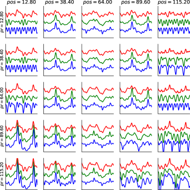
(a)    (b)

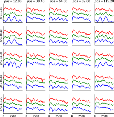
Figure 2: Output of $D1_{Z}2_{Y}$ as pressure $y_{0}$ and position $y_{1}$ are changed. Top (red) is the decoder with parameters explicitly specified and $z_{0}=0$; middle (green) is with parameters and $z_{0}$ inferred by the encoder, bottom (blue) is the dataset sample with closest parameters. (a) Time domain; (b) Frequency domain.

(a)    (b)

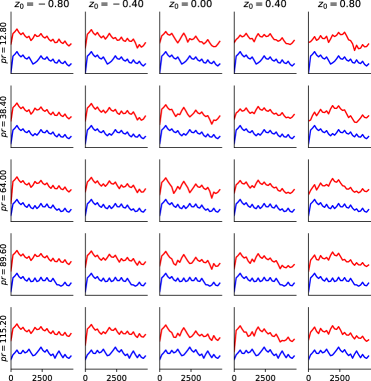
Figure 3: Output of $D1_{Z}2_{Y}$ as bow position is set to 100, and bow pressure and latent $z_{0}$ are changed. Top (red) Decoder output; bottom (blue) is the dataset. (a) Time domain; (b) Frequency domain.

6 Results

Figure 2 demonstrates the results of $D1_{Z}2_{Y}$. Comparing the middle and bottom curves, we can see that while it has some trouble with low values of bow pressure and the extremes of bow position, the autoencoder is able to more or less encode the distribution in our dataset. The top curve (red) was generated by explicitly specifying the $y$ (conditional) parameters instead of letting the autoencoder infer them, with $z_{0}=0$, and demonstrates the output for parameter-driven reconstruction if $z_{0}$ is held constant. Although not a perfect reproduction, particularly at extremes of the bow position range where there is more variance, this demonstrates that the trained network is able to approximate the data-parameter relationship present in the dataset.

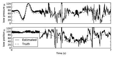
(a) (b)

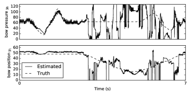
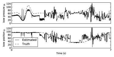
(c) (d)

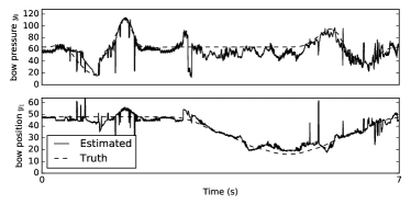
Figure 4: Parameter estimation performance of the $D1_{Z}2_{Y}$ network for (a) bowed1 full dataset, RMS error=23.23; (b) bowed1 half dataset, RMS error=33.45; (c) bowed2 full dataset, RMS error=19.54; (d) bowed2 half dataset, RMS error=8.61.

The role of $z$ is now considered in Figure 3, by holding bow position constant ($y_{1}=100$) and examining how the signal changes with $z_{0}$. One notices that for some values of $z_{0}$ the signal matches well, and for others it varies from the target signal. For example, we can see that in this case, high values of $z_{0}$ push the signal towards two sharp peaks, while low values of $z_{0}$ tend towards more oscillations; both $z_{0}=-0.8$ and $z_{0}=0.8$ resemble the $pr=115.2$ condition, but in different aspects. Meanwhile there is consistency with the “stylistic” influence of $z_{0}$ on the signal for different values of bow pressure; for lack of better words, in the time domain it changes from “peaky” to “wiggly” going from left to right.

Next, we look at the encoder (parameter estimator) performance, by producing a new signal from the STK synthesizer with a parameter trajectory starting with smooth variation only in bow pressure and then smooth variation only in bow position, and then in both parameters. Figure 4(a) shows actually rather disappointing performance in this respect, however it does clarify some information not present in the previous analysis: the estimation is clearly better for bow pressure, but easily disturbed by changes in bow position. Nonetheless we see the tendency of the estimate in the right direction, with rather a lot of flipping above and below the center. Since varying the hyperparameters of our network did not solve this problem, we hypothesized that this error could come from two sources: (1) ambiguities in the dataset—indeed, if one examines the shape of the signal as bow position changes, one notices a symmetry between values on either side of pos=64, c.f. samples from dataset in Figure 2, blue line. By consequence the inverse problem is underspecified, leading to ambiguity in the parameter estimate. (2) underrepresented variance in the dataset; the new testing data varies continuously in the parameters, but the dataset was constructed based on the per-parameter steady state.

To investigate this, the network was trained on a “half dataset”, consisting only of samples of bowed1 where bow position $<64$. Furthermore, as mentioned, an extended dataset, bowed2, was constructed based on random parameter variations. Results in Figure 4(b)-(d) show that training on the half-bowed1 dataset changed the character of errors, but did not improve overall, however the extended bowed2 dataset gave improved parameter estimation, and much improved in the bow position $<64$ case. Thus it can be concluded that both sources contributed to parameter estimation difficulties.

Figure 6 shows the resulting parameter space if both parameters are left to be absorbed by the unsupervised latent space. The adversarial regularization regime can be seen in the generator and discriminator losses of Fig. 6(b), which encourages the autoencoder to make the distribution of these variables similar to $\mathcal{U}(-1,1)$, i.e., a rectangle. This facilitates user interaction with the generator, since limited-range control knobs can be mapped to this rectangle, thus having a strong chance to access the full range of variance present in the dataset; conversely, the chance of synthesizing a sound that does not correspond with the training data is minimized. Without regularization, Fig. 6(a) ($N2_{Z}0_{Y}$), we see some relationship between the two inferred variables $z_{0}$ and $z_{1}$ (Fig. 6)—although it appears more complex than could be captured by a Pearson’s correlation—while this is completely gone for the regularized version ($D2_{Z}0_{y}$). The spreading clusters are generated because without regularization, the autoencoder attempts to maximally separate various aspects of the variance in a reduced 2-dimensional space in order to decrease uncertainty in reconstruction, which can be useful for data analysis but does not produce a good interpolation space. The regularization therefore encourages the parameter space to be interactively “interesting,” in the sense that the parameters represent orthogonal (or at least, uncorrelated) axes within the distribution that cover a defined domain (red square in Fig. 6) and tend towards uniform coverage without “holes”.

Of course, it is possible to restrict the domain without relying on the regularizer, simply by defining the network architecture accordingly. For instance, if the non-linear units are changed for the hyperbolic tangent, it is impossible for the network to generate values outside the range $[-1,1]$. In this sense the network architecture itself can be understood as contributing to regularization by enforcing hard constraints, rather than the soft constraints of the cost function. In Fig. 9, this tanh architecture is demonstrated on the bowed1 dataset, and it can be seen that the adversarial regularization nonetheless is still useful for ensuring that the domain is used effectively, i.e., despite some visual clusters still being apparent, they are much more spread out, better approximating a uniform distribution and, to a large degree, breaking up the piecewise correlations between the parameters that can be seen by inspection when regularization is not used. In general, we found the ReLU approach more stable and better at producing uniform coverage.

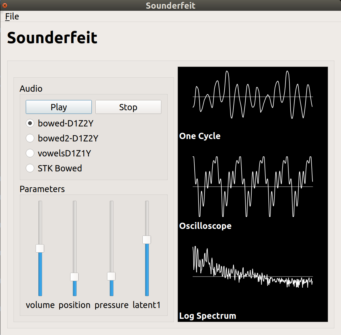
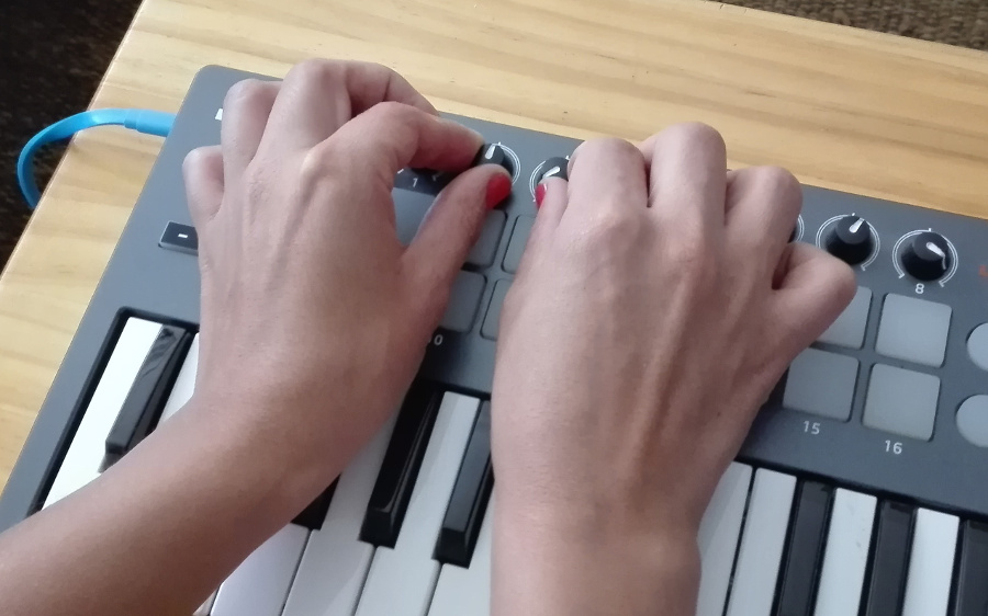
Figure 5: The Sounderfeit graphical user interface allows to interact in real time with the ANN-synthesized sound and compare it to the physical model that it was trained on. Here, pressure and position are controlled by limited-range knobs on a MIDI keyboard (Novation).

One will undoubtedly notice that the reconstruction error as reported in Fig. 6 does suffer due to the reguralization. Indeed this is an expected outcome since the regularization applies extra requirements such that the training will sacrifice one criteria to improve another. Additionally, the error will depend greatly on how much variance is present in the data vs. how much “room” it needs to express it—in this sense, we would expect accuracy to increase as latent dimensions are added. Fig. 9 gives an idea of how reconstruction error changes as we do so.

We found that with this small decoder network of 20300 weights and 300 biases, an overlap-add synthesis could be performed in real time on a laptop computer (10 seconds took 8.5 seconds to generate and was much faster when re-implemented in C++), and we can thus present a real-time, interactive data-driven wavetable synthesizer, which we call Sounderfeit, see Figure 5, with a number of adjustable parameters. The output of the overlap-add process is visualised in Figure 10.

Lastly, in order to verify this method on another dataset, a similar network was trained on the vowels dataset, adjusted to have the right size of input layer of 800, see Figure 9. The inferred space reflects the condition number (discrete, here), but the remaining parameter uniformly covers the range $[-1,1]$. In this case the extra variance beyond the conditional parameter consists only of small tonal changes in the recorded voice as well as microphone noise, and thus there is much more variance between vowels than within. It is apparent from Fig. 9(c) that there is no “leakage” of these extra sources of variance to the vowel label parameter axis, as the vowel number adequately identifies the cluster. The clusters can therefore be nicely mapped to a desired space automatically by the conditioning and regularization.

(a) Unregularized	(b) Adversarial regularization

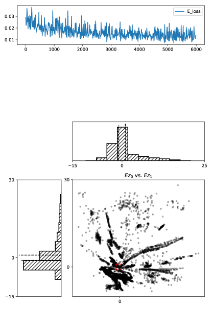
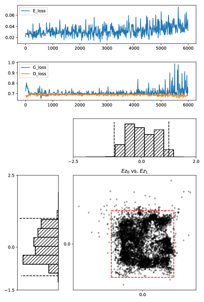
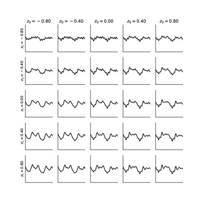
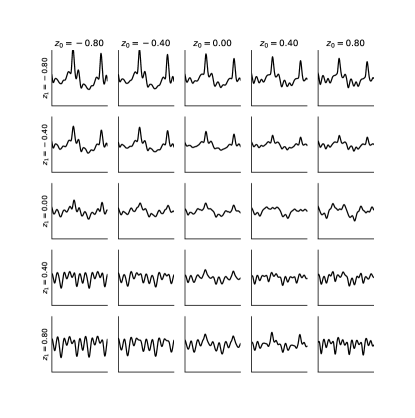
Figure 6: Distributions of latent parameters corresponding to a random sample of 3000 cycles from the dataset when trained (a) without regularization ($N2_{Z}0_{Y}$) and (b) with adversarial regularization ($D2_{Z}0_{Y}$). The top rows indicate reconstruction error ($E_{\textrm{loss}}$, mean square error in normalized representation), and adversarial discrimination errors ($G_{\textrm{loss}}=L_{G}$, $D_{\textrm{loss}}=L_{D}$). Regularization encourages the network to find a latent space such that the full variance of the dataset can be accessed uniformly from a restricted range of values, appropriate for interactive control.

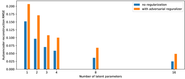
Figure 7: Reconstruction mean squared error as a function of the number of latent parameters, with and without reguralization.

(a) Unregularized	(b) Adversarial regularization

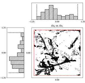
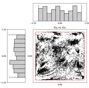
Figure 8: Results of same conditions as Fig. 6, but the ReLU activation functions are replaced with the hyperbolic tangent in order to restrict the domain of $z$ instead of relying on the regularizer. It can be seen that when the network architecture provides domain limiting, the regularization still provides a benefit of better approximating a uniform distribution, and further decorrelating the parameters.

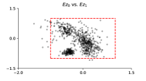
(a) (b) (c)

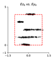
Figure 9: Results on vowels dataset: (a) using two latent parameters without regularization, the vowels are separated into clusters; (b) regularization encourages spreading to cover the uniform space within the desired boundaries, effectively smoothing out and blending the clusters; (c) replacing one latent parameter with conditioning on a vowel number 0 to 4.

7 Conclusions

These experiments showed some modest success in copying the parameter-data relationship of a physical modeling synthesizer and fitting them into a desired configuration. Like many machine learning approaches, the quality of results depends strongly on the hyperparameters used: network size and architecture, learning rates, regularization weights, etc., and these must be adapted to the dataset. Shown here are results from the best parameters found after some combination of automatic and manual optimisation on this specific dataset, which we use to demonstrate some principles of the design, however it should be noted that actual results varied sometimes unexpectedly with small changes to these parameters. This hyperparameter optimization is non-trivial, especially when it comes to audio where mean squared error may not reveal much about the perceptual quality of the results, and so a lot of trial and error is the game. Thus, a truly “universal”, turn-key synthesizer copier would require future work on measuring a combined hypercost that balances well the desire for good reproduction with good parameter estimation quality, and well-distributed latent parameters. Such work could go beyond mean squared error to involve perceptual models of sound perception. For example, recent work in speech synthesis has shown a significant improvement in perceived quality when the model was conditioned on mel frequency spectrograms [Shen et al. 2017].

Some practical notes: (1) We found that getting the adversarial method to properly regularize the latent variables in the presence of conditional variables is somewhat tricky; the batch size and relative learning rates played a lot in balancing the generator and discriminator performances. New research in adversarial methods is a current area of investigation in the ML community and many new techniques could apply here; moreover comparison with variational methods is needed—we note however that variational autoencoders are typically regularized to fit a Gaussian normal distribution, whereas an advantage of the adversarial approach is to fit any example-based distribution, which we took advantage of to fit the rectangle accessible by a pair of knobs. (2) We found the parameter estimation extremely sensitive to phase alignment; we tried randomizing phase of examples during training, which gave better parameter estimates, but this was quite damaging to the autoencoder performance. In general oversensitivity to global phase is a problem with this method, a downside to the time domain representation; more work on dealing with phase as a latent parameter is necessary.

Figure 10: Overlap-add output of $D1_{Z}2_{Y}$, varying each parameter over a short interval.

Nevertheless we have attempted to outline some potential for use of autoencoders and their latent spaces for audio analysis and synthesis based on a specific signal source. Only a very simple fully-connected single-layer architecture was used, and thus improvements should be explored, in particular the addition of convolutional layers. The advantages of time- and frequency-domain representations as learning targets should be characterised. More important than the quality of these specific results, we wish to point out the modular approach that autoencoders enable in modeling oscillator periods of known and unknown parameters, and that, in contrast to larger datasets covering many instruments [Engel et al. 2017], interesting insights and useful performance systems can be generated even from small data.

One might ask what a blackbox model brings to the table in the presence of an existing, semantically-rich physical model. Indeed, in this work a digital synthesizer was used as an easy way to gain access to a fairly complicated but clean signal with a small number of parameters. In principle this method could be used on much richer, real instrument recordings. To demonstrate this point we have trained it, as shown, on a very small vocal recording (3 seconds per vowel) and produced a working vowel synthesizer with separate knobs for vowel number and “noise”, e.g. microphone noise and vocal variance, however more complex experiments are needed in this vein. A challenge in operating on real data was cutting and aligning oscillation cycles correctly, which was non-trivial and prohibits easier experimentation on arbitrary data streams.

Simultaneous estimation and generation with the same network may be unnecessary. In fact conditioning variables could be made external inputs instead of inferred from the input data, and the decoder could be used separately to only learn the parameters in a more typical regression configuration. However, one of the long-term goals of performing automatic inference is to play somewhat with the latent and parameter space, such as using it for what is known in the audio community as cross-synthesis, or in the machine learning community as “style transfer”, i.e., swapping the bottom and top halves of two such autoencoder networks, allowing to drive a synthesizer by both conditioned and latent parameters estimated on an incoming signal. One can imagine, for example, playing the violin and having the bow pressure control the brightness of a wind instrument sound, while subtle aspects of the gesture are left to latent space to control more subtle parameters of the sound. To achieve this a much less noisy inference result would be necessary, and is of course predicated on the idea that the parameter to data function is invertible, which, as seen in our failure to map the complete bow position domain, is not necessarily a given. Another reason for doing simultaneous estimation and generation left for future work is to investigate whether a tied-weights approach might improve both goals by integrating mutual sources of information on either side of the equation.

Note

1. 1 Audio examples at: https://emac.ufg.br/up/269/o/Sinclair_soundexample.mp3.
2. 2 The learning rates have been changed from Sinclair2017sbcm: stochastic gradient descent with learning rate 0.005 for the autoencoder and learning rate 0.05 for the generator and discriminator. Due to a programming error, the autoencoder training step performed better with a different learning rate. We later found that the results were much more robust with the Adam optimiser and the same learning rate value for all training steps.
3. 3 Sounderfeit source code can be found on its project page at https://gitlab.com/sinclairs/sounderfeit

  Stephen Sinclair – In 2012 completed a PhD at McGill University in Montreal. His topic was audio-haptic interaction with musical acoustic models. He spent 3 years as a post-doctoral researcher in the ISIR laboratory of UPMC, Paris, working on new haptic interaction methods. Currently is a research engineer at Inria Chile, principally working to improve the Siconos non-smooth dynamical system simulation engine.

References

- [Abadi et al. 2015] ABADI, M; AGARWAL A; BARHAM P; BREVDO E; CHEN Z; CITRO C; CORRADO G; DAVIS A; DEAN J; DEVIN M; GHEMAWAT S; GOODFELLOW I; HARP A; IRVING G; ISARD M; JOZEFOWICZ R; JIA Y; KAISER L; KUDLUR M; LEVENBERG J; MANÉ D; SCHUSTER M; MONGA R; MOORE S; MURRAY D; OLAH C; SHLENS J; STEINER B; SUTSKEVER I; TALWAR K; TUCKER P; VANHOUCKE V; VASUDEVAN V; VIÉGAS F; VINYALS O; WARDEN P; WATTENBERG M; WICKE M; YU Y; ZHENG X, TensorFlow: Large-Scale Machine Learning on Heterogeneous Systems. 2015. Available: http://tensorflow.org. Accessed: 2017.
- [Cemgil e Erkut 1997] CEMGIL, A. T.; ERKUT, C, Calibration of physical models using artificial neural networks with application to plucked string instruments. In: Proceedings of the International Symposium on Musical Acoustics, St-Alban, UK, 1997. v. 19, p. 213–218.
- [Cook e Scavone 1999] COOK, P. R.; SCAVONE, G. P, The Synthesis ToolKit (STK). In: Proceedings of the International Compupater Music Conference, Beijing, china, 1999.
- [Engel et al. 2017] ENGEL, J; RESNICK, C; ROBERTS, A; DIELEMAN, S; ECK, D; SIMONYAN, K; NOROUZI, M, Neural audio synthesis of musical notes with WaveNet autoencoders. preprint arXiv:1704.01279, 2017.
- [Gabrielli et al. 2017] GABRIELLI, L; TOMASSETTI, S; SQUARTINI, S; ZINATO, C, Introducing deep machine learning for parameter estimation in physical modelling. Proceedings of the International Conference on Digital Audio Effects (DAFx-17), Edinburgh, UK, 2017.
- [Kingma e Ba 2015] KINGMA, D.; BA, J, Adam: A method for stochastic optimization. International Conference on Learning Representations, San Diego, 2015.
- [Makhzani et al. 2016] MAKHZANI, A; SHLENS, J; JAITLY, N; GOODFELLOW, I, Adversarial autoencoders. Proceedings of the International Conference on Learning Representations, San Juan, Puerto Rico, 2016.
- [Mehri et al. 2016] MEHRI, S; KUMAR, K; GULRAJANI, I; KUMAR, R; JAIN S; SOTELO, J; COURVILLE, A; BENGIO, Y, SampleRNN: An unconditional end-to-end neural audio generation model. International Conference on Learning Representations, Toulon, France, 2017.
- [Mirza e Osindero 2014] MIRZA, M.; OSINDERO, S, Conditional generative adversarial nets. arXiv preprint arXiv:1411.1784, 2014.
- [Oord et al. 2016] OORD, A; DIELEMAN, S; ZEN, H; SIMONYAN, K; VINYALS, O; GRAVES, A; KALCHBREN- NER, N; SENIOR, A; KAVUKCUOGLU, K, WaveNet: A generative model for raw audio. arXiv preprint arXiv:1609.03499, 2016.
- [Pfalz e Berdahl 2017] PFALZ, A.; BERDAHL, E. Toward inverse control of physics-based sound synthesis. Proceedings of the First International Conference on Deep Learning and Music, Anchorage, USA, 2017.
- [Radford, Metz e Chintala 2015] RADFORD, A.; METZ, L.; CHINTALA, S. Unsupervised representation learning with deep convolutional generative adversarial networks. Proceedings of the International Conference on Learning Representations, San Juan, Puerto Rico, 2016.
- [Riera, Eguía e Zabaljáuregui 2017] RIERA, P. E.; EGUÍA, M. C.; ZABALJÁUREGUI, M. Timbre spaces with sparse autoencoders. Proceedings of the Brazilian Symposium on Computer Music, Sao Paulo, Brazil, 2017. p. 93–98.
- [Riionheimo e Välimäki 2003] RIIONHEIMO, J.; VÄLIMÄKI, V. Parameter estimation of a plucked string synthesis model using a genetic algorithm with perceptual fitness calculation. EURASIP Journal on Advances in Signal Processing, Springer, v. 2003, n. 8, p. 758284, 2003.
- [Scherrer e Depalle 2011] SCHERRER, B.; DEPALLE, P. A physically-informed audio analysis framework for the identification of plucking gestures on the classical guitar. Canadian Acoustics, v. 39, n. 3, p. 132–133, 2011.
- [Shen et al. 2017] SHEN, J; PANG R; WEISS R; SCHUSTER M; JAITLY N; YANG Z; CHEN Z; ZHANG Y; WANG Y; SKERRY-RYAN, RJ, SAUROUS R; AGIOMYRGIANNAKIS Y; WU Y. Natural TTS synthesis by conditioning WaveNet on mel spectrogram predictions. arXiv preprint arXiv:1712.05884, 2017.
- [Sinclair 2017] SINCLAIR, S. Sounderfeit: Cloning a physical model with conditional adversarial autoencoders. Proceedings of the Brazilian Conference on Computer Music, Sao Paulo, Brazil, 2017. p. 67–74.
- [Smith e Serra 1987] SMITH, J; SERRA, X, PARSHL: An analysis/synthesis program for non-harmonic sounds ba- sed on a sinusoidal representation. Proceedings of the International Computer Music Conference, Tokyo, Japan, 1987.