Non-local cosmological models

Utkarsh Kumar^†

Indian Institute of Science Education and Research, Bhopal

Sukanta Panda^∗

Indian Institute of Science Education and Research, Bhopal

ABSTRACT

Nonlocal cosmological models are studied extensively in recent times because of their interesting cosmological consequences. In this paper, we have analyzed background cosmology on a class of non-local models which are motivated by the perturbative nature of gravity at infrared scale. We show that inflationary solutions are possible in all constructed non-local models. However, exit from inflation to RD era is not possible in most of the models.

^† e-mail: utkarshk@iiserb.ac.in

^∗ e-mail: sukanta@iiserb.ac.in

1 Introduction

Usually, we deal with local theories to study the cosmology of our universe. Generally, local theories contain a classical action which may be Einstien Hilbert(EH) action with matter or beyond. Our universe is accelerating in recent times as it is evident from supernovae observations [1]. To explain the acceleration of our current universe, a cosmological constant is usually added to the EH action. However, a physical picture describing the appearance of such a constant in a basic underlying theory is absent. To overcome such issue, other alternative models are floated by modifying the gravity or matter sector. Here in this paper, we work with purely modified gravity models. Our models are inspired by the nonlocal terms in the EH action which appear as IR corrections in gravity theory. In this connection, Infrared effects are calculated for de Sitter space in detail[2]. There are still issues in computing IR effects in de Sitter space[3, 4, 5, 6, 7]. Apart from these issues, a different approach is taken, which is phenomenological, to see the effect of nonlocal terms on the background cosmological evolution.

In the year 1998 Wetterich, first proposed a nonlocal gravity model with a nonlocal term as $\frac{1}{\Box}R$ and a dimensionless parameter [8]. This model did not produce correct cosmological background evolution. Much later in 2007, Deser and Woodard [9] modified the action with a nonlocal term as $Rf\left(\frac{1}{\Box}R\right),$ for more on this model refer to [10].In addition to above stated model, similar nonlocal models involving operators such as $R^{\mu\nu}\Box^{-1}G_{\mu\nu}$ have been presented by Barvinsky [11, 12, 13]. In these models all couplings are dimensionless. Another class of nonlocal models was introduced to study cosmology in IR regime where an additional mass scale corresponding to cosmological constant,$\Lambda$ arises [14, 15, 16, 17, 18].

The construction of phenomenological non local action is based on the behaviour of the theory in the parameter space where perturbation calculation around de-Sitter space is valid. Our nonlocal action is inspired from gravity correction to the hubble parameter in the perturbative regime in a de-Sitter space-time. Notation in this paper is same as that of ref. [19]. Perturbative IR corrected hubble parameter is given by [20, 21]

$$3H_{eff}^{2}=\Lambda+8\pi G\rho$$ (1)

$$H_{eff}(t)\,=\,H_{\rm in}\,\Big{\{}1-G\Lambda\Big{(}c_{2}G\Lambda\ln[a(t)]+c_{3}(G\Lambda)^{2}\ln^{2}[a(t)]+\dots\Big{)}\Big{\}}\;\;.$$ (2)

The perturbation result fails when $\ln a(t)\sim(G\Lambda)^{-1}$. To take an account of the IR correction of $O(\ln a(t))$, we need to introduce term $\frac{R}{\Box}$ into the action. In de Sitter space time it is shown that $\frac{R}{\Box}\simeq-4H_{in}t$ for large observation times [22]. However, beyond the perturbative limit, non-perturbative action can be modelled by a function $f(\frac{R}{\Box})$, so that we recover our perturbative results when $G\Lambda<<1$.

In terms of these corrections, the non-perturbative action takes form,

$$S=\int d^{4}x\sqrt{-g}\big{[}R+f(X)\big{]}$$ (3)

where $X=-G\Lambda\frac{1}{\Box}R$.

This was originally motivated to explain inflation in a purely gravitational action. This describes an inflation model followed by a very rapid reheating epoch. Here inflation is ended by a rapid oscillation of hubble parameter after which universe enters into radiation dominated era. However, this model experiences several problems like longer duration for inflation, inflation ends with rapid oscillations in hubble parameters, very fast reheating etc. For details refer to [20, 19].

To overcome these shortcomings in this model, a new model has been proposed in [19]. This model does not suffer from ”sign problem” as well as ”magnitude problem” as described in [19].(Sign problem is related to the graceful exit from inflation to radiation dominated era, where as magnitude problem is related to the theoretical value of $\Lambda$ which is quite large compared to its observed value at late times.) Then this model may describe unification of inflation era at very early times with dark energy dominated era at late times.

The paper is organised as follows. In section 2 we define the different non local models and derive the expressions required for background cosmological evolution. We have solved background evolution for five non local models and analyse their results in section 3-7. Finally we summarise all our findings in section 8.

2 Non-local Models

We study background cosmology in flat FRW metric given by

$$ds^{2}\;=\;-dt^{2}\,+\,a^{2}(t)\,d{\bf x}\cdot d{\bf x}\;\;.$$ (4)

where $a(t)$ is scale factor. Time variation of $a(t)$ gives the Hubble parameter and first slow roll parameter defined as

$$H(t)=\frac{\dot{a}(t)}{a(t)},$$ (5)

$$\epsilon(t)=1-\frac{a(t)\ddot{a}(t)}{\dot{a}^{2}(t)}=-\frac{\dot{H}(t)}{H^{2}(t)}.$$ (6)

The required curvature invariants for the our models in flat FRW metric are

$$R\,=\,6(2-\epsilon)H^{2}\quad,\quad R^{2}\,=\,36(2-\epsilon)^{2}H^{4}\;\;,$$ (7)

$$R_{\mu\nu}R^{\mu\nu}\,=\,12(3-3\epsilon+\epsilon^{2})H^{4}\;\;,$$ (8)

$$R_{\mu\nu\rho\sigma}R^{\mu\nu\rho\sigma}\,=\,12(2-2\epsilon+\epsilon^{2})H^{4}\;\;,$$ (9)

We also look for inverse differential Invariant operators that are responsible for nonlocalities and in FRW geometry they are expressed as

$$\Box=\frac{1}{\sqrt{-g}}\partial_{\mu}(\sqrt{-g}g^{\mu\nu}\partial_{\nu})=-\partial_{t}^{2}-3H\partial_{t}{\hskip 10.00002pt},$$ (10)

$$\Box_{c}=\Box-\frac{1}{6}R=-\partial_{t}^{2}-3H\partial_{t}-2H^{2}-\dot{H}{\hskip 10.00002pt},$$ (11)

while acting them to co-moving time. Their inverses are

$$\frac{1}{\Box}=\int_{t_{in}}^{t}dt^{{}^{\prime}}\frac{1}{a^{3}(t^{\prime})}\int_{t_{in}}^{t^{{}^{\prime}}}dt^{{}^{\prime\prime}}a^{3}(t^{{}^{\prime\prime}}){\hskip 10.00002pt},$$ (12)

$$\frac{1}{\Box}_{c}=\frac{1}{a(t)}\int_{t_{in}}^{t}dt^{{}^{\prime}}\frac{1}{a(t^{\prime})}\int_{t_{in}}^{t^{{}^{\prime}}}dt^{{}^{\prime\prime}}a^{2}(t^{{}^{\prime\prime}}){\hskip 10.00002pt},$$ (13)

these operators are defined with retarded boundary conditions to prevent the extra degree of freedom [25].

The model given in [19] takes the form

$$S=\int d^{4}x\sqrt{-g}\big{[}\frac{1}{16\pi G}R+f(X)\big{]},$$ (14)

where $X=G\frac{1}{\Box}R\frac{1}{\Box_{c}}\left(\frac{1}{3}R^{2}-R_{\mu\nu}R^{\mu\nu}\right)$ and $\Box_{c}=\Box-\frac{1}{6}R.$

We name this model as Model i@ throughout the paper. Here in our work, apart from this form of X[g], we consider other forms of X[g] that may be equally motivated phenomenologically. The proposed forms of X[g] are following:

$$(\@slowromancap ii@):{\hskip 20.00003pt}X[g]=G\frac{1}{\Box_{c}}R\frac{1}{\Box}\left(\frac{1}{3}R^{2}-R_{\mu\nu}R^{\mu\nu}\right),$$

$$(\@slowromancap iii@):{\hskip 20.00003pt}X[g]=G\frac{1}{\Box_{c}}\left(\frac{1}{3}R^{2}-R_{\mu\nu}R^{\mu\nu}\right)\frac{1}{\Box}R,$$

$$(\@slowromancap iv@):{\hskip 20.00003pt}X[g]=GR\frac{1}{\Box}\frac{1}{\Box_{c}}\left(\frac{1}{3}R^{2}-R_{\mu\nu}R^{\mu\nu}\right),$$

$$(\@slowromancap v@):{\hskip 20.00003pt}X[g]=G\left(\frac{1}{3}R^{2}-R_{\mu\nu}R^{\mu\nu}\right)\frac{1}{\Box}\frac{1}{\Box_{c}}R,$$

$$(\@slowromancap vi@):{\hskip 20.00003pt}X[g]=G\frac{1}{\Box}\frac{1}{\Box_{c}}R\left(\frac{1}{3}R^{2}-R_{\mu\nu}R^{\mu\nu}\right),$$

$$(\@slowromancap vii@):{\hskip 20.00003pt}X[g]=G\frac{1}{\Box_{c}}\frac{1}{\Box}R\left(\frac{1}{3}R^{2}-R_{\mu\nu}R^{\mu\nu}\right),$$

from equations (7) - (9) we get

$$\frac{1}{3}R^{2}-R_{\mu\nu}R^{\mu\nu}\,=\,12(1-\epsilon)H^{4}\;\;.$$ (15)

Equation (15) changes sign as $\epsilon$ passes through 1.

In this Paper we will not work with (vi@) and (vii@) forms of $X[g]$ since they give rise to unavoidable higher derivative of $\epsilon(>2)$ in the background equation of motion.

3 Model i@

For completeness, here we repeat the whole analysis done by [19]. Form of $X[g]$ considered in [19] is

$$X[g]=G\frac{1}{\Box}R\frac{1}{\Box_{c}}\left(\frac{1}{3}R^{2}-R_{\mu\nu}R^{\mu\nu}\right).$$ (16)

By introducing two auxilary scalar A,C and two lagrange multiplier B, D, we write equivalent scalar tensor lagrangian [23, 24] as

$$\begin{split}\mathcal{L}=&\Lambda^{2}h(GC)\sqrt{-g}+B\left[\Box_{c}A-\left(\frac{1}{3}R^{2}-R_{\mu\nu}R^{\mu\nu}\right)\right]\sqrt{-g}\\ &+D[\Box C-RA]\sqrt{-g}{\hskip 10.00002pt}.\end{split}$$ (17)

Varying equivalent lagrangian w.r.t auxilary and lagrange multiplier fields, we get

$$\frac{1}{\sqrt{-g}}\frac{\delta(\mathcal{L})}{\delta B}=\Box_{c}A-\left(\frac{1}{3}R^{2}-R_{\mu\nu}R^{\mu\nu}\right)=0{\hskip 10.00002pt},$$ (18)

$$\frac{1}{\sqrt{-g}}\frac{\delta(\mathcal{L})}{\delta D}=\Box C-RA=0{\hskip 10.00002pt},$$ (19)

$$\frac{1}{\sqrt{-g}}\frac{\delta(\mathcal{L})}{\delta A}=\Box_{c}B-RD=0{\hskip 10.00002pt}\Rightarrow B{\hskip 10.00002pt}=\frac{1}{\Box_{c}}RD{\hskip 10.00002pt},$$ (20)

$$\frac{1}{\sqrt{-g}}\frac{\delta(\mathcal{L})}{\delta C}=\Box D+G\Lambda^{2}h^{{}^{\prime}}(GC)=0{\hskip 10.00002pt}\Rightarrow{\hskip 10.00002pt}D=-\frac{1}{\Box}G\Lambda^{2}h^{{}^{\prime}}(GC){\hskip 10.00002pt}.$$ (21)

Equation of motion for fields for FRW metric canbe written in following forms

$${\ddot{A}} \!\!=\!\! -3H{\dot{A}}-(2-\epsilon)H^{2}A-12(1-\epsilon)H^{4}\;\;,$$ (22)

$${\ddot{B}} \!\!=\!\! -3H{\dot{B}}-(2-\epsilon)H^{2}B-6(2-\epsilon)H^{2}D\;\;,$$ (23)

$${\ddot{C}} \!\!=\!\! -3H{\dot{C}}-6(2-\epsilon)H^{2}A\;\;,$$ (24)

$${\ddot{D}} \!\!=\!\! -3H{\dot{D}}+G\Lambda^{2}h^{\prime}(GC)\;\;.$$ (25)

The $(00)$-component of Einstein field equations is

$$\begin{split}\frac{3H^{2}}{16\pi G}+\frac{1}{2}\Lambda^{2}h(GC)&-\frac{1}{2}(\dot{A}\dot{B}+\dot{C}\dot{D})-6H^{3}\dot{B}\\ -&3(H\partial_{t}+H^{2})(\frac{1}{6}AB+AD)=\frac{\Lambda}{16\pi G}{\hskip 10.00002pt},\end{split}$$ (26)

and $(11)$-component of Einstein field equation is

$$\begin{split}&-(3-2\epsilon)\frac{H^{2}}{16\pi G}-\frac{1}{2}\Lambda^{2}h(GC)+G\Lambda^{2}Ah^{\prime}(GC)-\frac{1}{6}\dot{A}\dot{B}-\frac{1}{2}\dot{C}\dot{D}+2\dot{A}\dot{D}\\ &{\hskip 10.00002pt}-2(1+2\epsilon)H^{3}\dot{B}-2(3-2\epsilon)H^{4}(B+6D)-(H\partial_{t}+H^{2})(\frac{1}{6}AB+AD)\\ &{\hskip 10.00002pt}=\frac{\Lambda}{16\pi G}{\hskip 10.00002pt}.\end{split}.$$ (27)

From equations (26) and (27), we find constraint equation for first slow roll parameter as

$$\begin{split}&\frac{2\epsilon H^{2}}{16\pi G}+G\Lambda^{2}Ah^{\prime}(GC)-\frac{2}{3}\dot{A}\dot{B}-\dot{C}\dot{D}+2\dot{A}\dot{D}-4(2+\epsilon)H^{3}\dot{B}\\ &{\hskip 10.00002pt}-2(3-2\epsilon)H^{4}(B+6D)-4(H\partial_{t}+H^{2})(\frac{1}{6}AB+AD)=0.\end{split}$$ (28)

In order to see the background evolution, we convert equations (22) -(28) into dimensionless form. We define dimensionless time as

$$\tau\equiv H_{in}t{\hskip 20.00003pt}\Rightarrow{\hskip 20.00003pt}\partial_{t}=H_{in}\partial_{\tau}.$$ (29)

Other dimensionless quantities involving Hubble parameter and scalar fields can also be defined as

$$H^{2}\equiv\frac{\chi^{2}}{G}{\hskip 20.00003pt}\Rightarrow{\hskip 20.00003pt}H^{2}_{in}\equiv\frac{\chi^{2}_{in}}{G}{\hskip 20.00003pt},{\hskip 20.00003pt}\Lambda\equiv 3H_{in}^{2}\equiv\frac{3\chi^{2}_{in}}{G}{\hskip 10.00002pt},$$ (30)

$$A\equiv-\frac{3\alpha}{G}{\hskip 20.00003pt},{\hskip 20.00003pt}B\equiv-3\beta{\hskip 20.00003pt},{\hskip 20.00003pt}C\equiv\frac{9\gamma}{G}{\hskip 20.00003pt},{\hskip 20.00003pt}D\equiv\delta{\hskip 10.00002pt},$$ (31)

$$h(GC)=h(9\gamma)\equiv f(\gamma){\hskip 10.00002pt}.$$ (32)

We wish to solve for $\left\{\alpha,\beta,\gamma,\delta,\chi,\epsilon\right\}$ subjected to following initial conditions at $\tau=\tau_{in}$,

$$\alpha=\alpha^{\prime}=\beta=\gamma=\gamma^{{}^{\prime}}=\delta^{{}^{\prime}}=\delta=0,\beta^{{}^{\prime}}=10,$$ (33)

$$\chi=\chi_{in},\epsilon=0.$$ (34)

where ${}^{\prime}=\frac{d}{d\tau}$

Using these dimensionless variables, equation of motion for $\left\{\alpha,\beta,\gamma,\delta\right\}$ can be cast as

$$\alpha^{{}^{\prime\prime}}+3\frac{\chi}{\chi_{in}}\alpha^{{}^{\prime}}+(2-\epsilon)\frac{\chi^{2}}{\chi^{2}_{in}}\alpha=4(1-\epsilon)\frac{\chi^{4}}{\chi^{2}_{in}}{\hskip 10.00002pt},$$ (35)

$$\beta^{{}^{\prime\prime}}+3\frac{\chi}{\chi_{in}}\beta^{{}^{\prime}}+(2-\epsilon)\frac{\chi^{2}}{\chi^{2}_{in}}\beta=2(2-\epsilon)\frac{\chi^{2}}{\chi^{2}_{in}}\delta{\hskip 10.00002pt},$$ (36)

$$\gamma^{{}^{\prime\prime}}+3\frac{\chi}{\chi_{in}}\gamma{{}^{\prime}}=2(2-\epsilon)\frac{\chi^{2}}{\chi^{2}_{in}}\alpha{\hskip 10.00002pt},$$ (37)

$$\delta^{{}^{\prime\prime}}+3\frac{\chi}{\chi_{i}n}\delta^{{}^{\prime}}=\chi_{in}^{2}f^{\prime}(\gamma){\hskip 10.00002pt},$$ (38)

Furthermore, the variable $\chi$ is obtained from equation (26)

$$\begin{split}\left[2\chi_{in}\beta^{{}^{\prime}}\right]\chi^{3}&+\left[\frac{1}{3}-\frac{1}{2}\alpha\beta+\alpha\delta\right]\chi^{2}+\chi_{in}\partial_{t}\left[--\frac{1}{2}\alpha\beta+\alpha\delta\right]\chi\\ &-\chi^{2}_{in}\left[\frac{1}{3}-\frac{1}{2}\chi_{in}^{2}f(\gamma)+\frac{1}{2}(\alpha^{{}^{\prime}}\beta^{{}^{\prime}}+\gamma^{{}^{\prime}}\delta^{{}^{\prime}})\right]=0{\hskip 10.00002pt},\end{split}$$ (39)

Moreover, we get equation for $\epsilon$ in terms of dimensionless variables from the equation(28) as

$$\begin{split}&\left[2\chi^{2}+12\chi_{in}\chi^{3}\beta^{{}^{\prime}}+12\chi^{4}(-\beta+2\delta)\right]\epsilon=3\Bigg{\{}\chi_{in}^{4}\alpha f^{\prime}(\gamma)+\chi_{in}^{2}(2\alpha^{\prime}\beta^{\prime}\\ &+3\gamma^{\prime}\delta^{\prime}+2\alpha^{\prime}\delta^{\prime})-8\chi_{in}\chi^{3}\beta^{\prime}-6\chi^{4}(\beta-2\delta)+4(\chi_{in}\chi\partial_{t}+\chi^{2})\left(\frac{1}{2}\alpha\beta-\alpha\delta\right)\Bigg{\}}\end{split}$$ (40)

Finally, we can further simplify equation (40) and we arrive at

$$\begin{split}\epsilon\chi^{2}&=\frac{3}{2+\beta^{\prime}\chi_{in}\chi+12(-\beta+2\delta)\chi^{2}}\times\\ &\Bigg{\{}\Big{[}\alpha f^{\prime}(\gamma)+2f(\gamma)\Big{]}\chi_{in}^{4}-\frac{4}{3}\chi_{in}^{2}+\Big{(}2\alpha^{\prime}+\gamma^{\prime}\Big{)}\delta^{\prime}\chi_{in}^{2}+\frac{4}{3}\chi^{2}+6(-\beta+2\delta)\chi^{4}\Bigg{\}}\end{split}$$ (41)

3.1 Results

Assuming scale factor to take its de Sitter value $a(\tau)=e^{{\tau}}$ during inflationary phase, all scalar fields decay as powers of $e^{\tau}$ which can be seen from following equations

$$\alpha(\tau) \!\!=\!\! 2\chi_{\rm in}^{2}\Bigl{(}1\!-\!e^{-\tau}\Bigr{)}^{2}\;\longrightarrow\;2\chi_{\rm in}^{2}\;,$$ (42)

$$\beta(\tau) \!\!=\!\! \frac{2}{3}\chi_{\rm in}^{2}\Bigl{(}\tau\!-\!\frac{11}{6}\!+\!3e^{-\tau}\!-\!\frac{3}{2}e^{-2\tau}\!+\!\frac{1}{3}e^{-3\tau}\Bigr{)}\;\longrightarrow\;\frac{2}{3}\chi_{\rm in}^{2}\Bigl{(}\tau\!-\!\frac{11}{6}\Bigr{)}\;,$$ (43)

$$\gamma(\tau) \!\!=\!\! \frac{8}{3}\chi_{\rm in}^{2}\Bigl{(}\tau\!-\!\frac{11}{6}\!+\!3e^{-\tau}\!-\!\frac{3}{2}e^{-2\tau}\!+\!\frac{1}{3}e^{-3\tau}\Bigr{)}\;\longrightarrow\;\frac{8}{3}\chi_{\rm in}^{2}\Bigl{(}\tau\!-\!\frac{11}{6}\Bigr{)}\;,$$ (44)

$$\delta(\tau) \!\!=\!\! \frac{1}{3}\chi_{\rm in}^{2}\Bigl{(}\tau\!-\!\frac{1}{3}\!+\!\frac{1}{3}e^{-3\tau}\Bigr{)}\;\longrightarrow\;\frac{1}{3}\chi_{\rm in}^{2}\Bigl{(}\tau\!-\!\frac{1}{3}\Bigr{)}\;.$$ (45)

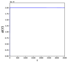
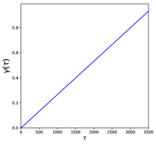
Figure 1: Plots for scalar field $\alpha(\tau)$ and $\gamma(\tau)$ for $\chi_{in}=\frac{1}{100}$ and $f(X)=\frac{X}{1-X}$.

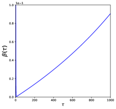
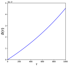
Figure 2: Plots for scalar field $\beta(\tau)$ and $\delta(\tau)$ for $\chi_{in}=\frac{1}{100}$ and $f(X)=\frac{X}{1-X}$.

Furthermore, using equations (42)-(45) derivatives of scalar fields during this epoch take the form

$$\alpha^{\prime}(\tau)\rightarrow 0{\hskip 10.00002pt},{\hskip 10.00002pt}\beta^{\prime}(\tau)\rightarrow\frac{2}{3}\chi_{in}^{2}{\hskip 10.00002pt},{\hskip 10.00002pt}\gamma^{\prime}(\tau)\rightarrow\frac{8}{3}\chi_{in}^{2}{\hskip 10.00002pt},{\hskip 10.00002pt}\delta^{\prime}(\tau)\rightarrow\frac{1}{3}\chi_{in}^{2}{\hskip 10.00002pt},$$ (46)

It is easy to obtain the values for the Hubble parameter and the slow roll parameter [19] as

$$\chi(\tau)\rightarrow\chi_{in}(1-2\chi_{in}^{4}\tau){\hskip 20.00003pt},{\hskip 20.00003pt}\epsilon(\tau)\rightarrow 2\chi_{in}^{4}{\hskip 10.00002pt}.$$ (47)

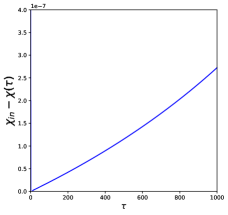
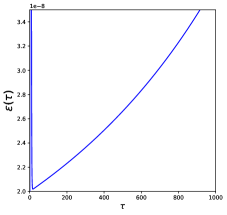
Figure 3: Plots for geometrical quantities $\chi_{in}-\chi(\tau)$ and $\epsilon(\tau)$ for $\chi_{in}=\frac{1}{100}$ and $f(X)=\frac{X}{1-X}$.

Figure 1 and 2 show well agreement between numerical and analytical result for values of $\tau=$ 0 to 3500 and $\tau=$ 0 to 1000 respectively. Figure 3 shows the compatibility between the expression given in equation (47) and numerical result for $\chi_{in}-\chi(t)$ and $\epsilon(t)$.

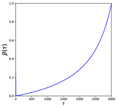
Figure 4: Plots for scalar fields $\beta(\tau)$ and $\delta(\tau)$ for $\chi_{in}=\frac{1}{100}$ and $f(X)=\frac{X}{1-X}$.

In Figure 4 the curvature appears from coupling between auxiliary scalars which are small during the deSitter epoch . First coupling is of $\delta(\tau)$ to $\gamma(\tau)$.Due to this coupling $\chi_{in}^{4}$ correction for $\delta(\tau)$ in (44) is given by

$$\delta(\tau)\rightarrow\frac{1}{3}\chi_{in}^{2}\tau+\frac{8}{9}\chi_{in}^{4}\tau^{2}\hskip 8.5359pt.$$ (48)

The curvature of $\beta(\tau)$ can be inferred from evolution of $\delta(\tau)$, it can be easily observed that $\chi_{in}^{4}$ correction to $\beta(\tau)$ is

$$\beta(\tau)\rightarrow\frac{2}{3}\chi_{in}^{2}\tau+\frac{16}{9}\chi_{in}^{4}\tau^{2}\hskip 8.5359pt.$$ (49)

The evolution of $\epsilon(\tau)$ is affected by the curvature of $\beta(\tau)$ and $\delta(\tau)$ which is evident in Figure 5. In turn, Hubble parameter decays much faster due to the curvature effects.

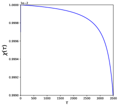
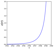
Figure 5: Plots Hubble parameter and the first slow roll parameter ($\epsilon$) for $\chi_{in}=\frac{1}{100}$ and $f(X)=\frac{X}{1-X}$.

In this model, inflation ends around $\tau\simeq 3750$ and transit to a RD epoch as $\epsilon$ rises above 1. After that there is no mechanism which can prevent further rise in $\epsilon$ and crosses over to Matter dominated or late-time acceleration epoch in this model.

4 Model ii@

Here $X[g]=G\frac{1}{\Box_{c}}R\frac{1}{\Box}\left(\frac{1}{3}R^{2}-R_{\mu\nu}R^{\mu\nu}\right)$. The equivalent Scalar tensor Lagrangian [23, 24] of action(14)

$$\begin{split}\mathcal{L}=&\Lambda^{2}h(GC)\sqrt{-g}+B\left[\Box A-\left(\frac{1}{3}R^{2}-R_{\mu\nu}R^{\mu\nu}\right)\right]\sqrt{-g}\\ &+D[\Box_{c}C-RA]\sqrt{-g}{\hskip 10.00002pt},\end{split}$$ (50)

where A and C are auxilary scalar fields and B and D are lagrange multiplier in the action.
Varying the action w.r.t both auxilary and lagrange multiplier fields, we get

$$\frac{1}{\sqrt{-g}}\frac{\delta(\mathcal{L})}{\delta B}=\Box A-\left(\frac{1}{3}R^{2}-R_{\mu\nu}R^{\mu\nu}\right)=0{\hskip 10.00002pt},$$ (51)

$$\frac{1}{\sqrt{-g}}\frac{\delta(\mathcal{L})}{\delta D}=\Box_{c}C-RA=0{\hskip 10.00002pt},$$ (52)

$$\frac{1}{\sqrt{-g}}\frac{\delta(\mathcal{L})}{\delta A}=\Box B-RD=0{\hskip 10.00002pt}\Rightarrow B{\hskip 10.00002pt}=\frac{1}{\Box}RD{\hskip 10.00002pt},$$ (53)

$$\frac{1}{\sqrt{-g}}\frac{\delta(\mathcal{L})}{\delta C}=\Box_{c}D+G\Lambda^{2}h^{{}^{\prime}}(GC)=0{\hskip 10.00002pt}\Rightarrow{\hskip 10.00002pt}D=-\frac{1}{\Box_{c}}G\Lambda^{2}h^{{}^{\prime}}(GC){\hskip 10.00002pt},$$ (54)

The equation of motion for fields (A,B,C,D) for FRW metric become

$${\ddot{A}} \!\!=\!\! -3H{\dot{A}}-12(1-\epsilon)H^{4}\;\;,$$ (55)

$${\ddot{B}} \!\!=\!\! -3H{\dot{B}}-6(2-\epsilon)H^{2}D\;\;,$$ (56)

$${\ddot{C}} \!\!=\!\! -3H{\dot{C}}-(2-\epsilon)H^{2}C-6(2-\epsilon)H^{2}A\;\;,$$ (57)

$${\ddot{D}} \!\!=\!\! -3H{\dot{D}}+G\Lambda^{2}h^{\prime}(GC)-(2-\epsilon)H^{2}D\;\;.$$ (58)

The $(00)$-component of Einstein field equations becomes

$$\begin{split}\frac{3H^{2}}{16\pi G}+\frac{1}{2}\Lambda^{2}h(GC)&-\frac{1}{2}(\dot{A}\dot{B}+\dot{C}\dot{D})-6H^{3}\dot{B}\\ -&3(H\partial_{t}+H^{2})(\frac{1}{6}CD+AD)=\frac{\Lambda}{16\pi G}{\hskip 10.00002pt},\end{split}$$ (59)

and $(11)$-component of Einstein equation provides

$$\begin{split}&-(3-2\epsilon)\frac{H^{2}}{16\pi G}-\frac{1}{2}\Lambda^{2}h(GC)+G\Lambda^{2}Ah^{\prime}(GC)\Big{(}A+\frac{1}{6}C\Big{)}-\frac{1}{6}\dot{C}\dot{D}\\ &-\frac{1}{2}\dot{A}\dot{B}+2\dot{A}\dot{D}{\hskip 10.00002pt}-2(1+2\epsilon)H^{3}\dot{B}-12(3-2\epsilon)H^{4}D\\ &-(H\partial_{t}+H^{2})(\frac{1}{6}CD+AD)=-\frac{\Lambda}{16\pi G}{\hskip 10.00002pt},\end{split}$$ (60)

Adding equation(59) and (60), we get

$$\begin{split}&\frac{2\epsilon H^{2}}{16\pi G}+G\Lambda^{2}Ah^{\prime}(GC)\Big{(}A+\frac{C}{6}\Big{)}-\frac{2}{3}\dot{C}\dot{D}-\dot{A}\dot{B}+2\dot{A}\dot{D}-4(2+\epsilon)H^{3}\dot{B}\\ &{\hskip 10.00002pt}-12(3-2\epsilon)H^{4}D-4(H\partial_{t}+H^{2})(\frac{1}{6}CD+AD)=0.\end{split}$$ (61)

In order to study the cosmological dynamics of this model, we use same set of dimensional parameters as Model i@

$$H^{2}\equiv\frac{\chi^{2}}{G}{\hskip 20.00003pt}\Rightarrow{\hskip 20.00003pt}H^{2}_{in}\equiv\frac{\chi^{2}_{in}}{G}{\hskip 20.00003pt},{\hskip 20.00003pt}\Lambda\equiv 3H_{in}^{2}\equiv\frac{3\chi^{2}_{in}}{G}{\hskip 10.00002pt},$$ (62)

$$A\equiv-\frac{3\alpha}{G}{\hskip 20.00003pt},{\hskip 20.00003pt}B\equiv-3\beta{\hskip 20.00003pt},{\hskip 20.00003pt}C\equiv\frac{9\gamma}{G}{\hskip 20.00003pt},{\hskip 20.00003pt}D\equiv\delta{\hskip 10.00002pt},$$ (63)

$$h(GC)=h(9\gamma)\equiv f(\gamma){\hskip 10.00002pt}.$$ (64)

The set of dimensionles parameters we wish to solve for is $\left\{\alpha,\beta,\gamma,\delta,\chi,\epsilon\right\}$ and is subjected to following initial conditions at $\tau=\tau_{in}$ :

$$\alpha=\alpha^{\prime}=\beta=\gamma=\gamma^{{}^{\prime}}=\delta^{{}^{\prime}}=\delta=0,\beta^{{}^{\prime}}=1.0{\hskip 20.00003pt},$$ (65)

$$\chi=\chi_{in},\epsilon=0{\hskip 10.00002pt}.$$ (66)

Now we write (55)-(58) in terms of dimensionless parameters

$$\alpha^{{}^{\prime\prime}}+3\frac{\chi}{\chi_{in}}\alpha^{{}^{\prime}}=4(1-\epsilon)\frac{\chi^{4}}{\chi^{2}_{in}}{\hskip 10.00002pt},$$ (67)

$$\beta^{{}^{\prime\prime}}+3\frac{\chi}{\chi_{in}}\beta^{{}^{\prime}}=2(2-\epsilon)\frac{\chi^{2}}{\chi^{2}_{in}}\delta{\hskip 10.00002pt},$$ (68)

$$\gamma^{{}^{\prime\prime}}+3\frac{\chi}{\chi_{in}}\gamma{{}^{\prime}}+(2-\epsilon)\frac{\chi^{2}}{\chi_{in}^{2}}\gamma=2(2-\epsilon)\frac{\chi^{2}}{\chi^{2}_{in}}\alpha{\hskip 10.00002pt},$$ (69)

$$\delta^{{}^{\prime\prime}}+3\frac{\chi}{\chi_{in}}\delta^{{}^{\prime}}+(2-\epsilon)\frac{\chi^{2}}{\chi_{in}^{2}}\delta=\chi_{in}^{2}f^{\prime}(\gamma){\hskip 10.00002pt},$$ (70)

Furthermore, the variable $\chi$ is obtained from the constraint equation (59) which takes the following form

$$\begin{split}\left[2\chi_{in}\beta^{{}^{\prime}}\right]\chi^{3}&+\left[\frac{1}{3}-\frac{1}{2}\gamma\delta+\alpha\delta\right]\chi^{2}+\chi_{in}\partial_{t}\left[-\frac{1}{2}\gamma\delta+\alpha\delta\right]\chi\\ &-\chi^{2}_{in}\left[\frac{1}{3}-\frac{1}{2}\chi_{in}^{2}f(\gamma)+\frac{1}{2}(\alpha^{{}^{\prime}}\beta^{{}^{\prime}}+\gamma^{{}^{\prime}}\delta^{{}^{\prime}})\right]=0{\hskip 10.00002pt}.\end{split}$$ (71)

Then, we solve $\epsilon$ in terms of dimensionless parameters from the equation (61)

$$\begin{split}&\left[2\chi^{2}+12\chi_{in}\chi^{3}\beta^{{}^{\prime}}+24\chi^{4}\delta\right]\epsilon=3\Bigg{\{}\chi_{in}^{4}f^{\prime}(\gamma)(\alpha-\frac{1}{2}\gamma)+\chi_{in}^{2}(3\alpha^{\prime}\beta^{\prime}+2\gamma^{\prime}\delta^{\prime}\\ &+2\alpha^{\prime}\delta^{\prime})+12\delta\chi^{4}-8\chi_{in}\chi^{3}\beta^{\prime}+4(\chi_{in}\chi\partial_{t}+\chi^{2})\left(\frac{1}{2}\gamma\delta-\alpha\delta\right)\Bigg{\}}\end{split}$$ (72)

Finally, we can further simplify equation (72) and we arrive at:

$$\begin{split}\epsilon\chi^{2}&=\frac{3}{2+12\beta^{\prime}\chi_{in}\chi+24\delta\chi^{2}}\times\\ &\Bigg{\{}\Big{[}f^{\prime}(\gamma)(\alpha-\frac{1}{2}\gamma)+2f(\gamma)\Big{]}\chi_{in}^{4}-\frac{4}{3}\chi_{in}^{2}+\Big{(}\beta^{\prime}+2\delta^{\prime}\Big{)}\delta^{\prime}\chi_{in}^{2}+\frac{4}{3}\chi^{2}+12\delta\chi^{4}\Bigg{\}}.\end{split}$$ (73)

4.1 Results

For a long time period $(\tau)$, performing similar calculations as in (3.1), scalar fields evolve as follows

$$\alpha(\tau) \!\!=\!\! \frac{4}{3}\chi_{in}^{2}\Big{(}\tau+\frac{e^{-3\tau}}{3}-\frac{1}{3}\Big{)}\longrightarrow\frac{4}{3}\chi_{in}^{2}\Big{(}\tau-\frac{1}{3}\Big{)}\;\;,$$ (74)

$$\beta(\tau) \!\!=\!\! \frac{4}{3}\chi_{\rm in}^{2}\Bigl{(}\tau\!-\!\frac{11}{6}\!+\!3e^{-\tau}\!-\!\frac{3}{2}e^{-2\tau}\!-\!\frac{1}{3}e^{-3\tau}\Bigr{)}\;\longrightarrow\;\frac{4}{3}\chi_{\rm in}^{2}\Bigl{(}\tau\!-\!\frac{11}{6}\Bigr{)}\;,$$ (75)

$$\gamma(\tau) \!\!=\!\! \frac{8}{3}\chi_{\rm in}^{2}\Bigl{(}\tau\!-\!\frac{11}{6}\!+\!3e^{-\tau}\!-\!\frac{3}{2}e^{-2\tau}\!-\!\frac{1}{3}e^{-3\tau}\Bigr{)}\;\longrightarrow\;\frac{8}{3}\chi_{\rm in}^{2}\Bigl{(}\tau\!-\!\frac{11}{6}\Bigr{)}\;,$$ (76)

$$\delta(\tau) \!\!=\!\! \frac{1}{2}\chi_{in}^{2}\bigg{(}1-e^{-\tau}\bigg{)}^{2}\longrightarrow\frac{1}{2}\chi_{in}^{2}\;.$$ (77)

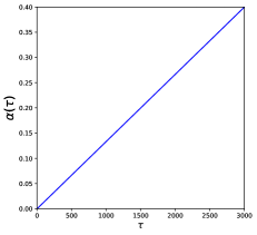
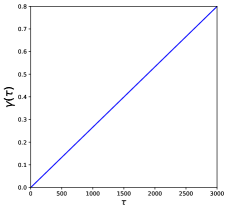
Figure 6: Plots for scalar field $\alpha(\tau)$ and $\gamma(\tau)$ for $\chi_{in}=\frac{1}{100}$ and $f(X)=\frac{X}{1-X}$ during the early epoch of de-Sitter expansion.

From the equations $(\ref{earlyalpham1})-(\ref{earlydeltam1})$, derivative of auxilary fields during this phase can be derived as

$$\alpha^{\prime}(\tau)\longrightarrow\frac{4}{3}\chi_{in}^{2}\;\;,\;\;\beta^{\prime}(\tau)\longrightarrow\frac{4}{3}\chi_{in}^{2}\;\;,\;\;\gamma^{\prime}(\tau)\longrightarrow\frac{8}{3}\chi_{\rm in}^{2}\;\;,\;\;\delta^{\prime}(\tau)\longrightarrow 0\;.$$ (78)

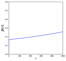
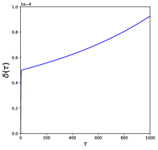
Figure 7: Plots for scalar field $\beta(\tau)$ and $\delta(\tau)$ for $\chi_{in}=\frac{1}{100}$ and $f(X)=\frac{X}{1-X}$ during the early epoch of de-Sitter expansion.

Using expression of field variables and their derivatives, corresponding Hubble parameter and the effective equation of state $(w_{eff})$ evolve as follows:

$$\chi(\tau)\longrightarrow\chi_{in}(1-2\chi_{in}^{4}\tau)\hskip 28.45274pt,\hskip 28.45274ptw_{eff}\equiv-1+\frac{2}{3}\epsilon\hskip 8.5359pt.$$ (79)

Numerically we plot evolution of field variables in Figure 6 and 7 from $\tau=0$ to 3000 and $\tau=0$ to 1000 respectively.At long times, from Figure 6, we observe that the expressions (74) and (76) match with numerical plot. Similarly, from Figure 7, it is clear that expressions for field variables (75) and (77) also agree with our numerical calculation roughly for short time period. We plot $\beta$ and $\delta$ in Figure 8 and obtained curvature in their plot can be explained by the coupling of auxilary scalar fields.

There are two coupling present in the system. First is of $\beta(\tau)$ to $\delta(\tau)$ which can be seen as

$$\beta^{\prime\prime}=-3\frac{\chi}{\chi_{in}}\beta^{\prime}+2(2-\epsilon)\frac{\chi^{2}}{\chi_{in}^{2}}\delta\longrightarrow-3\beta^{\prime}+4\delta$$ (80)

Solving equation (80), which provides order $\chi_{[n}^{4}$corrections to the field $\beta$.

$$\beta(\tau)\longrightarrow\chi_{in}^{4}\tau^{2}\hskip 14.22636pt.$$ (81)

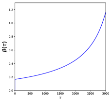
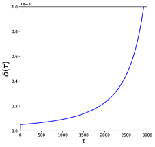
Figure 8: Plots for scalar field $\beta(\tau)$ and $\delta(\tau)$ for $\chi_{in}=\frac{1}{100}$ and $f(X)=\frac{X}{1-X}$ during the early epoch of de-Sitter expansion.

While equation (81) shows a rough agreemment to left hand plot of Figure 8 , one can find a perfect fit by choosing the exponent of $\tau$ as $2.24$ of $\chi_{in}^{4}$ order.

The variation of $\delta(\tau)$ can be understood from the second coupling of $\delta(\tau)$ to $\gamma(\tau)$ from equation (70) while assuming $f(X)=\frac{X}{1-X}$    .

$$\delta^{\prime\prime}=-3\frac{\chi}{\chi^{2}_{in}}\delta^{\prime}-(2-\epsilon)\frac{\chi^{2}}{\chi_{in}^{2}}\delta+\chi_{in}^{2}\hskip 2.84544pt\textit{f}\hskip 2.84544pt(X)\longrightarrow-3\delta^{\prime}+\chi_{in}^{2}(1+2\gamma)\hskip 14.22636pt.$$ (82)

Now the $\chi_{in}^{6}$ correction appears in $\delta(\tau)$ as

$$\delta(\tau)\longrightarrow\frac{1}{2}\chi_{in}^{2}+\frac{4}{27}\chi_{in}^{6}\tau^{3}\hskip 14.22636pt.$$ (83)

R.H.S. plot of Figure 8 shows rough agreement to equation (83) .

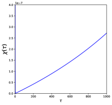
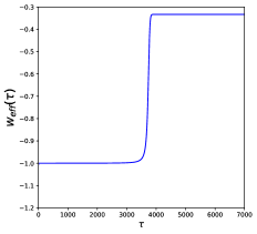
Figure 9: Plots for geometric quantities $\chi_{in}^{2}-\chi$ and $w_{eff}$ for $\chi_{in}=\frac{1}{100}$ and $f(X)=\frac{X}{1-X}$ during the early epoch of de-Sitter expansion.

The effect of curvature of $\beta(\tau)$ and $\delta(\tau)$ is to evolve the values of $\epsilon$ = 0 to 1 at late-times. From Figure 9, it can be observed that $w_{eff}=-1$ stays for a long time period and eventually it increases to $w_{eff}=-0.33$ and stays there forever.

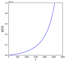
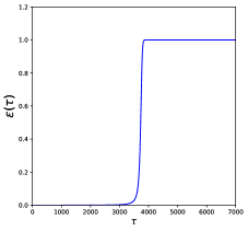
Figure 10: Plots for geometric quantities $\epsilon(\tau)$ for $\chi_{in}=\frac{1}{100}$ and $f(X)=\frac{X}{1-X}$ Left hand plot shows the variation of $\epsilon(\tau)$ during the early epoch of nearly de Sitter expansion. Right hand plot shows the variation after that epoch and up to $\tau=7000$.

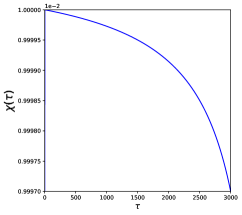
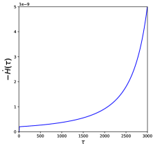
Figure 11: Plots for geometric quantities $H(\tau)$ and its first derivative for $\chi_{in}=\frac{1}{100}$ and $f(X)=\frac{X}{1-X}$.

Figure 11 shows the Hubble parameter and its first derivative .

5 Model iii@

In this case $X[g]$ becomes

$$X[g]=G\frac{1}{\Box_{c}}\left(\frac{1}{3}R^{2}-R_{\mu\nu}R^{\mu\nu}\right)\frac{1}{\Box}R$$ (84)

Equivalent scalar tensor lagrangian can be written as follows

$$\begin{split}\mathcal{L}=&\Lambda^{2}h(GC)\sqrt{-g}+B\left[\Box A-R\right]\sqrt{-g}\\ &+D[\Box_{c}C-\left(\frac{1}{3}R^{2}-R_{\mu\nu}R^{\mu\nu}\right)A]\sqrt{-g}{\hskip 10.00002pt},\end{split},$$ (85)

where A and C are auxilary scalar fields and B and D are lagrange multiplier in the action.
Varying the action w.r.t both auxilary and lagrange multiplier fields, we get

$$\frac{1}{\sqrt{-g}}\frac{\delta(\mathcal{L})}{\delta B}=\Box A-R=0{\hskip 10.00002pt},$$ (86)

$$\frac{1}{\sqrt{-g}}\frac{\delta(\mathcal{L})}{\delta D}=\Box_{c}C-\left(\frac{1}{3}R^{2}-R_{\mu\nu}R^{\mu\nu}\right)A=0{\hskip 10.00002pt},$$ (87)

$$\frac{1}{\sqrt{-g}}\frac{\delta(\mathcal{L})}{\delta A}=\Box B-\left(\frac{1}{3}R^{2}-R_{\mu\nu}R^{\mu\nu}\right)D=0{\hskip 10.00002pt}\Rightarrow B{\hskip 10.00002pt}=\frac{1}{\Box}\left(\frac{1}{3}R^{2}-R_{\mu\nu}R^{\mu\nu}\right)D{\hskip 10.00002pt},$$ (88)

$$\frac{1}{\sqrt{-g}}\frac{\delta(\mathcal{L})}{\delta C}=\Box_{c}D+G\Lambda^{2}h^{{}^{\prime}}(GC)=0{\hskip 10.00002pt}\Rightarrow{\hskip 10.00002pt}D=-\frac{1}{\Box_{c}}G\Lambda^{2}h^{{}^{\prime}}(GC){\hskip 10.00002pt},$$ (89)

The equation of motion for fields(A,B,C,D) for FRW metric in this model becomes

$${\ddot{A}} \!\!=\!\! -3H{\dot{A}}-6(2-\epsilon)H^{2}\;\;,$$ (90)

$${\ddot{B}} \!\!=\!\! -3H{\dot{B}}-12(1-\epsilon)H^{4}D\;\;,$$ (91)

$${\ddot{C}} \!\!=\!\! -3H{\dot{C}}-(2-\epsilon)H^{2}C-12(1-\epsilon)H^{4}A\;\;,$$ (92)

$${\ddot{D}} \!\!=\!\! -3H{\dot{D}}+G\Lambda^{2}h^{\prime}(GC)-(2-\epsilon)H^{2}D\;\;.$$ (93)

The $(00)$-component of modified Einstein field equation is

$$\begin{split}\frac{3H^{2}}{16\pi G}+\frac{1}{2}\Lambda^{2}h(GC)&-\frac{1}{2}(\dot{A}\dot{B}+\dot{C}\dot{D})-6H^{3}\dot{A}D-6H^{3}\dot{D}A\\ -&3(H\partial_{t}+H^{2})(\frac{1}{6}CD+B)=\frac{\Lambda}{16\pi G}{\hskip 10.00002pt},\end{split}$$ (94)

and $(11)$-component of field equation is

$$\begin{split}&-(3-2\epsilon)\frac{H^{2}}{16\pi G}-\frac{1}{2}\Lambda^{2}h(GC)+G\Lambda^{2}Ah^{\prime}(GC)\Big{(}2A+\frac{1}{6}C\Big{)}-\frac{1}{6}\dot{C}\dot{D}-\frac{1}{2}\dot{A}\dot{B}+4\dot{A}\dot{D}H^{2}\\ &{\hskip 10.00002pt}-2(1+2\epsilon)H^{3}(\dot{A}D+\dot{D}A)-12(3-2\epsilon)H^{4}D-(H\partial_{t}+H^{2})\frac{1}{6}CD-2\epsilon BH^{2}\\ &-2(3-2\epsilon)H^{4}AD+3H^{2}B-H\partial_{t}B{\hskip 10.00002pt}=-\frac{\Lambda}{16\pi G}{\hskip 10.00002pt}.\end{split}$$ (95)

Adding equations (94) and (95), we obtain

$$\begin{split}&\frac{2\epsilon H^{2}}{16\pi G}+G\Lambda^{2}Ah^{\prime}(GC)\Big{(}2A+\frac{C}{6}\Big{)}-\frac{2}{3}\dot{C}\dot{D}-\dot{A}\dot{B}+4\dot{A}\dot{D}H^{2}\\ &{\hskip 10.00002pt}-12(3-2\epsilon)H^{4}D-4(H\partial_{t}+H^{2})\frac{1}{6}CD-4H\partial_{t}B-2\epsilon BH^{2}\\ &-4(2+\epsilon)H^{3}(\dot{A}D+\dot{D}A)-2(3-2\epsilon)H^{4}AD=0\end{split}$$ (96)

To convert equations (90) - (96) into dimensionless equations, we use a different set of dimensionless parameters i.e. $\left\{\alpha,\beta,\gamma,\delta\right\}$ as:

$$A\equiv-3\alpha{\hskip 20.00003pt},{\hskip 20.00003pt}B\equiv\frac{-3\beta}{G}{\hskip 20.00003pt},{\hskip 20.00003pt}C\equiv\frac{9\gamma}{G}{\hskip 20.00003pt},{\hskip 20.00003pt}D\equiv\delta{\hskip 10.00002pt},$$ (97)

$$h(GC)=h(9\gamma)\equiv f(\gamma){\hskip 10.00002pt}.$$ (98)

We solve equation for $\left\{\alpha,\beta,\gamma,\delta,\chi,\epsilon\right\}$ numerically subjected to following initial conditions at $\tau=\tau_{in}$ :

$$\alpha=\alpha^{\prime}=\beta=\gamma=\gamma^{{}^{\prime}}=\delta^{{}^{\prime}}=\delta=0,\beta^{{}^{\prime}}=0{\hskip 20.00003pt},$$ (99)

$$\chi=\chi_{in}{\hskip 20.00003pt},{\hskip 20.00003pt}\epsilon=0{\hskip 10.00002pt}.$$ (100)

Using these dimensionless variables, equation of motion for $\left\{\alpha,\beta,\gamma,\delta\right\}$ cast as :

$$\alpha^{{}^{\prime\prime}}+3\frac{\chi}{\chi_{in}}\alpha^{{}^{\prime}}=2(2-\epsilon)\frac{\chi^{2}}{\chi^{2}_{in}}{\hskip 10.00002pt},$$ (101)

$$\beta^{{}^{\prime\prime}}+3\frac{\chi}{\chi_{in}}\beta^{{}^{\prime}}=4(1-\epsilon)\frac{\chi^{4}}{\chi^{2}_{in}}\delta{\hskip 10.00002pt},$$ (102)

$$\gamma^{{}^{\prime\prime}}+3\frac{\chi}{\chi_{in}}\gamma{{}^{\prime}}+(2-\epsilon)\frac{\chi^{2}}{\chi_{in}^{2}}\gamma=4(1-\epsilon)\frac{\chi^{4}}{\chi^{2}_{in}}\alpha{\hskip 10.00002pt},$$ (103)

$$\delta^{{}^{\prime\prime}}+3\frac{\chi}{\chi_{i}n}\delta^{{}^{\prime}}+(2-\epsilon)\frac{\chi^{2}}{\chi_{in}^{2}}\delta=\chi_{in}^{2}f^{\prime}(\gamma){\hskip 10.00002pt},$$ (104)

The constraint equation for $\chi$ in terms of dimensionless variables is derived from equation (94) as

$$\begin{split}2\chi_{in}\left[\alpha^{\prime}\delta+\delta^{\prime}\alpha\right]\chi^{3}&+\left[\frac{1}{3}-\frac{1}{2}\gamma\delta+\beta\right]\chi^{2}-\chi_{in}\partial_{t}\left[\frac{1}{2}\gamma\delta-\beta\right]\chi\\ &-\chi^{2}_{in}\left[\frac{1}{3}-\frac{1}{2}\chi_{in}^{2}f(\gamma)+\frac{1}{2}(\alpha^{{}^{\prime}}\beta^{{}^{\prime}}+\gamma^{{}^{\prime}}\delta^{{}^{\prime}})\right]=0{\hskip 10.00002pt},\end{split}$$ (105)

We solve for $\epsilon$ from the equation (96) as

$$\begin{split}&\epsilon\Big{[}2\chi^{2}+6\beta\chi^{2}-12\chi^{4}\Big{(}\alpha\delta-2\delta\Big{)}+12\Big{(}\alpha^{\prime}\delta-\alpha\delta^{\prime}\Big{)}\chi_{in}\chi^{3}\Big{]}=3\Bigg{\{}\chi^{4}_{in}f^{\prime}(\gamma)\Big{(}3\alpha-\frac{3}{2}\delta\Big{)}\\ &+\chi_{in}^{2}\{3\alpha^{\prime}\beta^{\prime}+2\gamma^{\prime}\delta^{\prime}+4\alpha^{\prime}\delta^{\prime}\chi^{2}\}-8\chi_{in}\chi^{3}\left[\alpha^{\prime}\delta+\alpha\delta^{\prime}\right]-6\chi^{4}(\alpha\delta-2\delta)-4\chi\chi_{in}\beta^{\prime}\\ &+2\Big{(}\chi\chi_{in}\partial_{t}+\chi^{2}\Big{)}\gamma\delta\Bigg{\}}.\end{split}$$ (106)

Finally, we can further simplify equation (106) to arrive at

$$\begin{split}\epsilon\chi^{2}&=\frac{3}{\Big{[}2+6\beta-12\chi^{2}\Big{(}\alpha\delta-2\delta\Big{)}+12\Big{(}\alpha^{\prime}\delta-\alpha\delta^{\prime}\Big{)}\chi_{in}\chi\Big{]}}\times\\ &\Bigg{\{}\chi^{4}_{in}[f^{\prime}(\gamma)(2\alpha-\frac{3}{2}\delta)+2f(\gamma)]+\chi_{in}^{2}(\alpha^{\prime}\beta^{\prime}+4\alpha^{\prime}\delta^{\prime}\chi^{2})\\ &+\frac{4}{3}(\chi^{2}-\chi^{2}_{in})+(4\chi^{2}+\chi_{in}\chi\partial_{t})\beta-6\chi^{4}(\alpha\delta-2\delta)\Bigg{\}}.\end{split}$$ (107)

5.1 Results

Here we perform a similar analysis campared to model i@ and ii@. In this model scalar fields are approximated, for large values of $\tau$, as

$$\alpha(\tau) \!\!=\!\! \frac{4}{3}\chi_{in}^{2}\Big{(}\tau+\frac{e^{-3\tau}}{3}-\frac{1}{3}\Big{)}\longrightarrow\frac{4}{3}\chi_{in}^{2}\Big{(}\tau-\frac{1}{3}\Big{)}\;\;,$$ (108)

$$\beta(\tau) \!\!=\!\! \frac{4}{3}\chi_{\rm in}^{2}\Bigl{(}\tau\!-\!\frac{11}{6}\!+\!3e^{-\tau}\!-\!\frac{3}{2}e^{-2\tau}\!-\!\frac{1}{3}e^{-3\tau}\Bigr{)}\;\longrightarrow\;\frac{4}{3}\chi_{\rm in}^{2}\Bigl{(}\tau\!-\!\frac{11}{6}\Bigr{)}\;,$$ (109)

$$\gamma(\tau) \!\!=\!\! \frac{8}{3}\chi_{\rm in}^{2}\Bigl{(}\tau\!-\!\frac{11}{6}\!+\!3e^{-\tau}\!-\!\frac{3}{2}e^{-2\tau}\!-\!\frac{1}{3}e^{-3\tau}\Bigr{)}\;\longrightarrow\;\frac{8}{3}\chi_{\rm in}^{2}\Bigl{(}\tau\!-\!\frac{11}{6}\Bigr{)}\;,$$ (110)

$$\delta(\tau) \!\!=\!\! \frac{1}{2}\chi_{in}^{2}\bigg{(}1-e^{-\tau}\bigg{)}^{2}\longrightarrow\frac{1}{2}\chi_{in}^{2}\;.$$ (111)

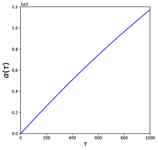
Figure 12: Plots for scalar field $\alpha(\tau)$ for $\chi_{in}=\frac{1}{100}$ and $f(X)=\frac{X}{1-X}$.

Similar to our previous analysis, Figure 12 shows the matching of our numerical result with the expression for $\alpha(\tau)$ in equation (108).

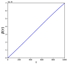
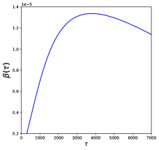
Figure 13: Plots for scalar field $\beta(\tau)$ for $\chi_{in}=\frac{1}{100}$ and $f(X)=\frac{X}{1-X}$.

Similarly plots for $\beta(\tau)$ in Figure 13 also match with our numerical and analytical expression from $\beta(\tau)$ in equation (109). Curvature in $\beta(\tau)$ shows up for values of $\tau>1000$.

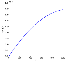
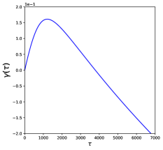
Figure 14: Plots for scalar field $\gamma(\tau)$ for $\chi_{in}=\frac{1}{100}$ and $f(X)=\frac{X}{1-X}$.

$\gamma(\tau)$ initially increases with $\tau$ and around $\tau\simeq 1300$ it shows a decaying trend as seen in Figure 14. Using the fact that $f(X[g])=\frac{X}{1-X}$ becomes singular at X = 1 where inflation ends as shown in the case of Model i@ [19]. In current model this value X = 1 corresponds to a value of $\tau=3752.33$.

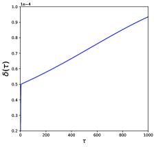
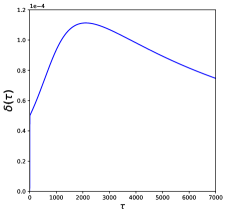
Figure 15: Plots for scalar field $\delta(\tau)$ for $\chi_{in}=\frac{1}{100}$ and $f(X)=\frac{X}{1-X}$.

Figure 15 shows the behaviour of scalar field $\delta(\tau)$. It attains its maximum at $\tau=2110.27$ and decreases beyond this value. In order to see the late time behaviour, we determine the derivatives of auxilary fields during de-Sitter epoch as

$$\alpha^{\prime}(\tau)\longrightarrow\frac{4}{3}\;\;,\;\;\beta^{\prime}(\tau)\longrightarrow\frac{4}{3}\chi_{in}^{4}\;\;,\;\;\gamma^{\prime}(\tau)\longrightarrow\frac{8}{3}\chi_{\rm in}^{2}\;\;,\;\;\delta^{\prime}(\tau)\longrightarrow 0\;.$$ (112)

Using these derivatives and equations (105) and (107) to the expressions for Hubble parameter and the the first slow roll parameter as

$$\chi(\tau)\longrightarrow\chi_{in}(1-\chi_{in}^{5}\tau)\hskip 14.22636pt,\hskip 14.22636pt\epsilon(\tau)\longrightarrow 5\chi_{in}^{2}\tau$$ (113)

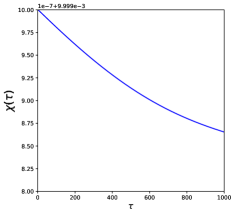
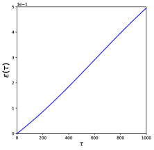
Figure 16: Plots for Geometric quantities $\chi(\tau)$ and $\epsilon(\tau)$ for $\chi_{in}=\frac{1}{100}$ and $f(X)=\frac{X}{1-X}$.

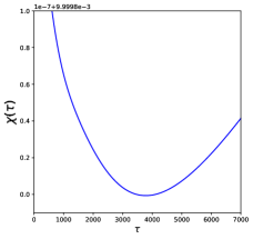
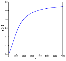
Figure 17: Plots for Geometric quantities $\chi(\tau)$ and $\epsilon(\tau)$ for $\chi_{in}=\frac{1}{100}$ and $f(X)=\frac{X}{1-X}$.

The behaviour of $\chi(\tau)$ and $\epsilon(\tau)$ are plotted in Figure 16 and 17 for $\tau$ from $0$ to $1000$ and for $\tau$ from 0 to 7000 respectively. It turns out that at late-times $\epsilon\longrightarrow 1$ and remains to that value thereafter. This corresponds to equation of state $w_{eff}=-\frac{1}{3}$. The exit from inflation to Radiation Dominated epoch will never be achieved in this case.

6 Model iv@

Model iv@ has $X[g]$ of form

$$X[g]=GR\frac{1}{\Box}\frac{1}{\Box_{c}}\left(\frac{1}{3}R^{2}-R_{\mu\nu}R^{\mu\nu}\right)$$ (114)

In this case we will restrict ourself to particular form of $h(X[g])=X[g]$ . Any other form of $h(X[g])$ will lead to higher derivaive in the equation of motion.
For $h(X[g])=X[g]$, lagrangian is written as

$$\begin{split}\mathcal{L}=&\Lambda^{2}GRC\sqrt{-g}+B\left[\Box_{c}A-\left(\frac{1}{3}R^{2}-R_{\mu\nu}R^{\mu\nu}\right)\right]\sqrt{-g}\\ &+D[\Box C-A]\sqrt{-g}{\hskip 10.00002pt},\end{split}$$ (115)

To write langrangian (115) in equivalent scalar-tensor lagrangian, we introduce two auxilary scalar fields A and C and two lagrange multiplier B and D which obeys following equations of motion

$$\frac{1}{\sqrt{-g}}\frac{\delta(\mathcal{L})}{\delta B}=\Box_{c}A-\left(\frac{1}{3}R^{2}-R_{\mu\nu}R^{\mu\nu}\right)=0{\hskip 10.00002pt},$$ (116)

$$\frac{1}{\sqrt{-g}}\frac{\delta(\mathcal{L})}{\delta D}=\Box C-A=0{\hskip 10.00002pt},$$ (117)

$$\frac{1}{\sqrt{-g}}\frac{\delta(\mathcal{L})}{\delta A}=\Box_{c}B-D=0{\hskip 10.00002pt}\Rightarrow B{\hskip 10.00002pt}=\frac{1}{\Box_{c}}D{\hskip 10.00002pt},$$ (118)

$$\frac{1}{\sqrt{-g}}\frac{\delta(\mathcal{L})}{\delta C}=\Box D+\Lambda^{2}GRC=0{\hskip 10.00002pt}\Rightarrow{\hskip 10.00002pt}D=-\frac{1}{\Box}G\Lambda^{2}R{\hskip 10.00002pt},$$ (119)

Equation of motion for fields (A,B,C,D) using FRW metric can be as

$${\ddot{A}} \!\!=\!\! -3H{\dot{A}}-(2-\epsilon)H^{2}A-12(1-\epsilon)H^{4}\;\;,$$ (120)

$${\ddot{B}} \!\!=\!\! -3H{\dot{B}}-(2-\epsilon)H^{2}B-D\;\;,$$ (121)

$${\ddot{C}} \!\!=\!\! -3H{\dot{C}}-A\;\;,$$ (122)

$${\ddot{D}} \!\!=\!\! -3H{\dot{D}}+G\Lambda^{2}R\;\;.$$ (123)

Now taking the variation of lagrangian with respect to metric and using the F.R.W. geometry, $(00)$-component of field equations becomes

$$\begin{split}\frac{3H^{2}}{16\pi G}+3H^{2}(\Lambda^{2}G)C&+3H\partial_{t}(\Lambda^{2}GC)-\frac{1}{2}(\dot{A}\dot{B}+\dot{C}\dot{D})-6H^{3}\dot{B}\\ -&3(H\partial_{t}+H^{2})\frac{1}{6}AB+\frac{1}{2}AD=\frac{\Lambda}{16\pi G}{\hskip 10.00002pt},\end{split}$$ (124)

and $(11)$-component becomes

$$\begin{split}&-(3-2\epsilon)\frac{H^{2}}{16\pi G}-(3-2\epsilon)H^{2}(\Lambda^{2}GC)+H\partial_{t}(\Lambda^{2}GC)+G\Lambda^{2}A-\frac{1}{6}\dot{A}\dot{B}-\frac{1}{2}\dot{C}\dot{D}\\ &{\hskip 10.00002pt}-2(1+2\epsilon)H^{3}\dot{B}-2(3-2\epsilon)H^{4}B-(H\partial_{t}+H^{2})\frac{1}{6}AB-2DH^{2}-\frac{1}{3}AD\\ &{\hskip 10.00002pt}=\frac{\Lambda}{16\pi G}{\hskip 10.00002pt},\end{split}$$ (125)

Now adding equations (124) and (125), we find

$$\begin{split}&\frac{2\epsilon H^{2}}{16\pi G}+2\epsilon H^{2}(\Lambda^{2}GC)+4H\partial_{t}(\Lambda^{2}GC)+\Lambda^{2}GA-\frac{2}{3}\dot{A}\dot{B}-\dot{C}\dot{D}\\ &{\hskip 10.00002pt}-2(3-2\epsilon)H^{4}B-4(2+\epsilon)H^{3}\dot{B}-4(H\partial_{t}+H^{2})\frac{1}{6}AB-2DH^{2}-\frac{1}{6}AD=0\end{split}$$ (126)

To convert equations (120) -(126) in to dimensionless equations, we use different set of dimensionless parameters i.e. $\left\{\alpha,\beta,\gamma,\delta\right\}$ defined as:

$$A\equiv\frac{-3\alpha}{G}{\hskip 20.00003pt},{\hskip 20.00003pt}B\equiv-3\beta{\hskip 20.00003pt},{\hskip 20.00003pt}C\equiv 3\gamma{\hskip 20.00003pt},{\hskip 20.00003pt}D\equiv\frac{9\delta}{G}{\hskip 10.00002pt},.$$ (127)

The set of dimensionles parameters we wish to solve for are $\left\{\alpha,\beta,\gamma,\delta,\chi,\epsilon\right\}$, which are subjected to following initial conditions at $\tau=\tau_{in}$ :

$$\alpha=\alpha^{\prime}=\beta=\gamma=\gamma^{{}^{\prime}}=\delta^{{}^{\prime}}=\delta=0,\beta^{{}^{\prime}}=10{\hskip 20.00003pt},$$ (128)

$$\chi=\chi_{in}{\hskip 20.00003pt},{\hskip 20.00003pt}\epsilon=0{\hskip 10.00002pt}.$$ (129)

Using these dimensionless variables, equation of motion for $\left\{\alpha,\beta,\gamma,\delta\right\}$ can be written in following forms :

$$\alpha^{{}^{\prime\prime}}+3\frac{\chi}{\chi_{in}}\alpha^{{}^{\prime}}+(2-\epsilon)\frac{\chi^{2}}{\chi^{2}_{in}}\alpha=4(1-\epsilon)\frac{\chi^{4}}{\chi^{2}_{in}}{\hskip 10.00002pt}$$ (130)

$$\beta^{{}^{\prime\prime}}+3\frac{\chi}{\chi_{in}}\beta^{{}^{\prime}}+(2-\epsilon)\frac{\chi^{2}}{\chi^{2}_{in}}\beta=\frac{3\delta}{\chi^{2}_{in}}{\hskip 10.00002pt},$$ (131)

$$\gamma^{{}^{\prime\prime}}+3\frac{\chi}{\chi_{in}}\gamma{{}^{\prime}}=\frac{\alpha}{\chi^{2}_{in}}{\hskip 10.00002pt},$$ (132)

$$\delta^{{}^{\prime\prime}}+3\frac{\chi}{\chi_{i}n}\delta^{{}^{\prime}}=6\chi_{in}^{2}\chi^{2}(2-\epsilon){\hskip 10.00002pt},$$ (133)

Furthermore, the variable $\chi$ is obtained from equation (124);

$$\begin{split}\left[2\chi_{in}\beta^{{}^{\prime}}\right]\chi^{3}&+\left[\frac{1}{3}+9\gamma\chi_{in}^{4}-\frac{1}{2}\alpha\beta\right]\chi^{2}+\chi_{in}\partial_{t}\left[-\frac{1}{2}\alpha\beta+9\chi_{in}^{4}\gamma\right]\chi\\ &-\chi^{2}_{in}\left[\frac{1}{3}+\frac{1}{2}\alpha^{{}^{\prime}}\beta^{{}^{\prime}}+\frac{3}{2}\gamma^{{}^{\prime}}\delta^{{}^{\prime}}-\frac{3}{2}\alpha\delta\right]=0{\hskip 10.00002pt},\end{split}$$ (134)

Moreover, we solve for $\epsilon$ from the constraint equation (126) and we get :

$$\begin{split}\epsilon\chi^{2}&=\frac{3}{2+54\chi_{in}^{2}\gamma+12\beta\chi^{2}-12\chi\chi_{in}\beta^{\prime}}\times\\ &\Bigg{\{}9\chi_{in}^{2}\alpha-9\alpha\delta-18\chi^{2}\beta+18\chi^{2}\delta+\frac{4}{3}\chi^{3}-\frac{4}{3}\chi_{in}^{2}+36\chi_{in}^{4}\chi^{4}\gamma+3\chi_{in}\gamma^{\prime}\delta^{\prime}\Bigg{\}}.\end{split}$$ (135)

6.1 Results

Here we perform a similar analysis campared to model i@ and ii@. In this model scalar fields are approximated, for large values of $\tau$, as

$$\alpha(\tau) \!\!=\!\! 2\chi_{\rm in}^{2}\Bigl{(}1\!-\!e^{-\tau}\Bigr{)}^{2}\;\longrightarrow\;2\chi_{\rm in}^{2}\;,$$ (136)

$$\beta(\tau) \!\!=\!\! \frac{1}{6}\chi_{\rm in}^{2}\Bigl{(}\tau\!-\!\frac{3}{2}\!+\!3e^{-\tau}\!-\!\frac{3}{2}e^{-2\tau}\Bigr{)}\;\longrightarrow\;\frac{1}{6}\chi_{\rm in}^{2}\Bigl{(}\tau\!-\!\frac{3}{2}\Bigr{)}\;,$$ (137)

$$\gamma(\tau) \!\!=\!\! \frac{2}{3}\Bigl{(}\tau\!-\!\frac{11}{6}\!+\!3e^{-\tau}\!-\!\frac{3}{2}e^{-2\tau}\!-\!\frac{1}{3}e^{-3\tau}\Bigr{)}\;\longrightarrow\;\frac{2}{3}\Bigl{(}\tau\!-\!\frac{11}{6}\Bigr{)}\;,$$ (138)

$$\delta(\tau) \!\!=\!\! 4\chi_{\rm in}^{4}\Bigl{(}\tau\!-\!\frac{1}{3}\!+\!\frac{1}{3}e^{-3\tau}\Bigr{)}\;\longrightarrow\;4\chi_{\rm in}^{2}\Bigl{(}\tau\!-\!\frac{1}{3}\Bigr{)}\;.$$ (139)

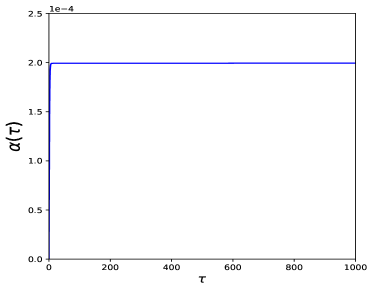
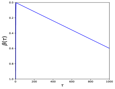
Figure 18: Plots for scalar field $\alpha(\tau)$ and $\beta(\tau)$ for $\chi_{in}=\frac{1}{100}$ and $f(X)=X$.

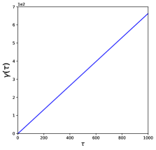
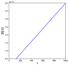
Figure 19: Plots for scalar field $\gamma(\tau)$ and $\delta(\tau)$ for $\chi_{in}=\frac{1}{100}$ and $f(X)=X$.

Figure 18 and Figure 19 shows a rough agreement with the (136) - (139). Unlike other models here the effect of the coupling between $\gamma(\tau)$ and $\alpha(\tau)$ ,$\beta(\tau)$ and between $\delta(\tau)$ is not significant enough to provide any curvature in the behaviour of scalar fields as seen in Figure 18 and 19. In this case derivative of auxilary scalar fields $\alpha,\beta,\gamma,\delta$ becomes

$$\alpha^{\prime}(\tau)\longrightarrow 0\;\;,\;\;\beta^{\prime}(\tau)\longrightarrow\frac{1}{6}\chi_{\rm in}^{2}\;\;,\;\;\gamma^{\prime}(\tau)\longrightarrow\frac{2}{3}\;\;,\;\;\delta^{\prime}(\tau)\longrightarrow 4\chi_{\rm in}^{4}\;.$$ (140)

From these derivatives, we can draw conclusions regarding the behaviour of $\chi(\tau)$ and $\epsilon(\tau)$. It is evident in Figure 20 that $\epsilon\longrightarrow$ 1 after a very long $\tau$. In our case this happens for $\tau=10^{6}$. Similar to Model iii@, exit from inflation to RD era is also not possible in this model.

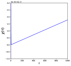
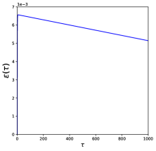
Figure 20: Plots for Geometric quantities $\chi(\tau)$ and $\epsilon(\tau)$ and $w_{eff}$ for $\chi_{in}=\frac{1}{100}$ and $f(X)=X$.

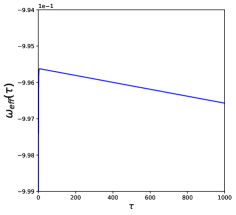
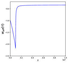
Figure 21: Plots for Geometric quantities $\chi(\tau)$ and $\epsilon(\tau)$ and $w_{eff}$ for $\chi_{in}=\frac{1}{100}$ and $f(X)=X$.

7 Model v@

Here, we consider following form of $X[g]$

$$X[g]=G\left(\frac{1}{3}R^{2}-R_{\mu\nu}R^{\mu\nu}\right)\frac{1}{\Box}\frac{1}{\Box_{c}}R$$ (141)

In this case we will also restrict ourself to particular form of $h(X[g])=X[g]$ . Similar to Model ($\@slowromancap iv@$)any other form of $h(X[g])$ will give rise to higher derivative in the equation of motion.
For $h(X[g])=X[g]$, lagrangian is written as

$$\begin{split}\mathcal{L}=&\Lambda^{2}h(GC)\left(\frac{1}{3}R^{2}-R_{\mu\nu}R^{\mu\nu}\right)\sqrt{-g}+B\left[\Box_{c}A-R\right]\sqrt{-g}\\ &+D[\Box C-A]\sqrt{-g}{\hskip 10.00002pt},\end{split}$$ (142)

Here we introduce two auxilary scalar fields A, C and two lagrange multiplier B, D , to convert nonlocal lagrangian into local one, which obeys following equation of motion :

$$\frac{1}{\sqrt{-g}}\frac{\delta(\mathcal{L})}{\delta B}=\Box_{c}A-R=0{\hskip 10.00002pt},$$ (143)

$$\frac{1}{\sqrt{-g}}\frac{\delta(\mathcal{L})}{\delta D}=\Box C-A=0{\hskip 10.00002pt},$$ (144)

$$\frac{1}{\sqrt{-g}}\frac{\delta(\mathcal{L})}{\delta A}=\Box_{c}B-D=0{\hskip 10.00002pt}\Rightarrow B{\hskip 10.00002pt}=\frac{1}{\Box_{c}}D{\hskip 10.00002pt},$$ (145)

$$\frac{1}{\sqrt{-g}}\frac{\delta(\mathcal{L})}{\delta C}=\Box D+\Lambda^{2}G\left(\frac{1}{3}R^{2}-R_{\mu\nu}R^{\mu\nu}\right)=0{\hskip 10.00002pt}\Rightarrow{\hskip 10.00002pt}D=-\frac{1}{\Box_{c}}\Lambda^{2}G\left(\frac{1}{3}R^{2}-R_{\mu\nu}R^{\mu\nu}\right){\hskip 10.00002pt},$$ (146)

The equation of motion for fields for FRW metric can be written as

$${\ddot{A}} \!\!=\!\! -3H{\dot{A}}-(2-\epsilon)H^{2}A-6(2-\epsilon)H^{2}\;\;,$$ (147)

$${\ddot{B}} \!\!=\!\! -3H{\dot{B}}-(2-\epsilon)H^{2}B-D\;\;,$$ (148)

$${\ddot{C}} \!\!=\!\! -3H{\dot{C}}-A\;\;,$$ (149)

$${\ddot{D}} \!\!=\!\! -3H{\dot{D}}+12\Lambda^{2}G(1-\epsilon)H^{4}\;\;.$$ (150)

Now taking the variation of lagrangian with respect to metric and using the F.R.W. geometry $(00)$ component of field equations is

$$\begin{split}\frac{3H^{2}}{16\pi G}+6H^{3}\dot{C}(\Lambda^{2}G)&-\frac{1}{2}(\dot{A}\dot{B}+\dot{C}\dot{D})\\ -&3(H\partial_{t}+H^{2})(\frac{1}{6}AB+B)-\frac{1}{2}AD=\frac{\Lambda}{16\pi G}{\hskip 10.00002pt},\end{split}$$ (151)

and $(11)$-component is :

$$\begin{split}-(3-2\epsilon)\frac{H^{2}}{16\pi G}&+2H^{3}(1+2\epsilon)\dot{C}(\Lambda^{2}G)-2H^{2}A(\Lambda^{2}G)-\frac{1}{6}\dot{A}\dot{B}-\frac{1}{2}\dot{C}\dot{D}\\ &-(H^{2}+H\partial_{t})(\frac{1}{6}AB+B)-\frac{1}{6}AD-D=-\frac{\Lambda}{16\pi G},\end{split}$$ (152)

Now addition of (151) and (152) leads to :

$$\begin{split}&\frac{2\epsilon H^{2}}{16\pi G}+4H^{3}(2+\epsilon)(\Lambda^{2}G)\dot{C}-2H^{2}A(\Lambda^{2}G)-\frac{2}{3}\dot{A}\dot{B}-\dot{C}\dot{D}\\ &{\hskip 20.00003pt}-4(H^{2}+H\partial_{t})(\frac{1}{6}AB+B)-\frac{1}{6}AD=0\end{split}$$ (153)

To convert equations (147) -(153) into dimensionaless equations, we use set of dimensionless parameters i.e. $\left\{\alpha,\beta,\gamma,\delta\right\}$ defined as:

$$A\equiv-3\alpha,{\hskip 20.00003pt}B\equiv\frac{-9\beta}{G}{\hskip 20.00003pt},{\hskip 20.00003pt}C\equiv 3\gamma G{\hskip 20.00003pt},{\hskip 20.00003pt}D\equiv\frac{9\gamma}{G^{2}}{\hskip 10.00002pt},.$$ (154)

The set of dimensionles parameters we wish to solve for $\left\{\alpha,\beta,\gamma,\delta,\chi,\epsilon\right\}$ is subjected to following initial conditions at $\tau=\tau_{in}$ :

$$\alpha=\alpha^{\prime}=\beta=\beta^{{}^{\prime}}=\gamma=\delta^{{}^{\prime}}=\delta=0,\gamma^{{}^{\prime}}=10,$$ (155)

$$\chi=\chi_{in},\epsilon=0.$$ (156)

Using these dimensionless variables equation of motion for $\left\{\alpha,\beta,\gamma,\delta\right\}$ can be cast as

$$\alpha^{{}^{\prime\prime}}+3\frac{\chi}{\chi_{in}}\alpha^{{}^{\prime}}+(2-\epsilon)\frac{\chi^{2}}{\chi^{2}_{in}}\alpha=2(2-\epsilon)\frac{\chi^{2}}{\chi^{2}_{in}}{\hskip 10.00002pt},$$ (157)

$$\beta^{{}^{\prime\prime}}+3\frac{\chi}{\chi_{in}}\beta^{{}^{\prime}}+(2-\epsilon)\frac{\chi^{2}}{\chi_{in}^{2}}\beta=\frac{\delta}{\chi_{in}^{2}}{\hskip 10.00002pt},$$ (158)

$$\gamma^{{}^{\prime\prime}}+3\frac{\chi}{\chi_{in}}\gamma{{}^{\prime}}=\frac{\alpha}{\chi^{2}_{in}}{\hskip 10.00002pt},$$ (159)

$$\delta^{{}^{\prime\prime}}+3\frac{\chi}{\chi_{i}n}\delta^{{}^{\prime}}=12(1-\epsilon)\chi_{in}^{2}\chi^{4}{\hskip 10.00002pt},$$ (160)

Furthermore, the variable $\chi$ is solved from the dimensionless form of the $(00)$ component of field equation

$$\begin{split}\left[6\chi_{in}^{5}\gamma^{{}^{\prime}}\right]\chi^{3}&+\left[\frac{1}{9}-\frac{1}{2}\alpha\beta+\beta\right]\chi^{2}+\chi_{in}\partial_{t}\left[-\frac{1}{2}\alpha\beta+\beta\right]\chi\\ &-\chi^{2}_{in}\left[\frac{1}{9}-\frac{1}{2}(\alpha^{{}^{\prime}}\beta^{{}^{\prime}}+\gamma^{{}^{\prime}}\delta^{{}^{\prime}})\right]=0{\hskip 10.00002pt},\end{split}$$ (161)

Moreover, we solve for $\epsilon$ from the equation (153) and we get :

$$\begin{split}\epsilon\chi^{2}&{\hskip 20.00003pt}=\frac{9}{\Big{[}2+108\chi_{in}^{5}\chi\gamma^{\prime}\Big{]}}\times\\ &\Bigg{\{}\frac{4}{9}\chi^{2}-\frac{4}{9}\chi_{in}^{2}-2\chi_{in}^{2}\alpha^{\prime}\beta^{\prime}-6\chi_{in}^{4}\chi^{2}\alpha+3\chi_{in}^{2}\gamma^{\prime}\delta^{\prime}+\delta+2\delta\alpha)\Bigg{\}}.\end{split}$$ (162)

7.1 Results

Here we perform a similar analysis compared to previous models. For this model, scalar fields are approximated, for large values of $\tau$, as

$$\alpha(\tau) \!\!=\!\! 2\!+\!2e^{-2\tau}\!-\!4e^{-\tau}\;\longrightarrow\;2\;,$$ (163)

$$\beta(\tau) \!\!=\!\! 2\chi_{\rm in}^{4}\Bigl{(}\tau\!-\!\frac{11}{6}\!-\!\frac{1}{3}e^{-3\tau}\!-\!\frac{3}{2}e^{-2\tau}\!+\!3e^{-\tau}\Bigr{)}\;\longrightarrow\;2\chi_{\rm in}^{4}\Bigl{(}\tau\!-\!\frac{11}{6}\Bigr{)}\;,$$ (164)

$$\gamma(\tau) \!\!=\!\! \frac{2}{3}\chi_{in}^{-2}\Bigl{(}\tau\!-\!\frac{11}{6}\!+\!\frac{1}{3}e^{-3\tau}\!-\!\frac{3}{2}e^{-2\tau}\!+\!3e^{-\tau}\Bigr{)}\;\longrightarrow\;\frac{2}{3}\chi_{in}^{-2}\Bigl{(}\tau\!-\!\frac{11}{6}\Bigr{)}\;,$$ (165)

$$\delta(\tau) \!\!=\!\! 4\chi_{\rm in}^{6}\Bigl{(}\tau\!-\!\frac{1}{3}\!+\!\frac{1}{3}e^{-3\tau}\Bigr{)}\;\longrightarrow\;4\chi_{\rm in}^{6}\Bigl{(}\tau\!-\!\frac{1}{3}\Bigr{)}\;.$$ (166)

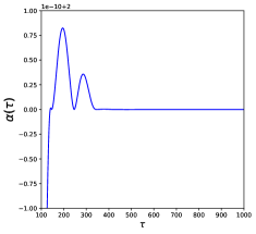
Figure 22: Plots for scalar field $\alpha(\tau)$ and $\beta(\tau)$ for $\chi_{in}=\frac{1}{100}$ and $f(X)=X$.

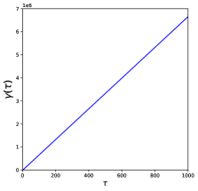
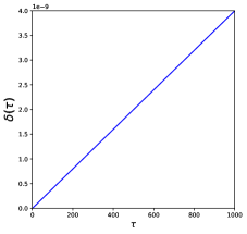
Figure 23: Plots for scalar field $\gamma(\tau)$ and $\delta(\tau)$ for $\chi_{in}=\frac{1}{100}$ and $f(X)=X$.

Figure 22 shows behaviour of auxilary scalars $\alpha(\tau)$ and $\beta(\tau)$ in time range $0\leq\tau\leq 1000$ . Examining the Figure 22 in the time range $\tau\leq 400$, we find that field $\alpha(\tau)$ shows small peaks around $2.0000005$ while $\beta(\tau)$ shows a linear dependence. Numerical results for sclar fields $\gamma(\tau)$ and $\delta(\tau)$ match with analytical expressions (165) and (166).

From relations (163) -(166) we compute expressions for first derivative of auxilary salar fields during de Sitter epoch as

$$\alpha^{\prime}(\tau)\longrightarrow 0\;\;,\;\;\beta^{\prime}(\tau)\longrightarrow 2\chi_{\rm in}^{4}\;\;,\;\;\gamma^{\prime}(\tau)\longrightarrow\frac{2}{3}\chi_{in}^{-2}\;\;,\;\;\delta^{\prime}(\tau)\longrightarrow 4\chi_{\rm in}^{6}\;.$$ (167)

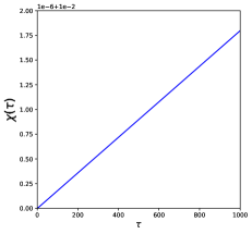
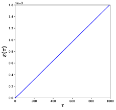
Figure 24: Plots for Geometric quantities $\chi(\tau)$ and $\epsilon(\tau)$ for $\chi_{in}=\frac{1}{100}$ and $f(X)=X$.

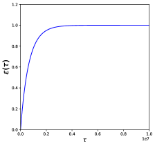
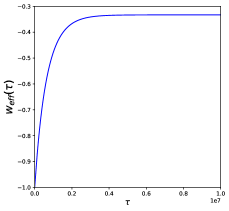
Figure 25: Plots for Geometric quantities $\epsilon(\tau)$ and $w_{eff}(\tau)$ for $\chi_{in}=\frac{1}{100}$ and $f(X)=X$.

Figure 24 shows numerical simulation of the $\chi(\tau)$ and $\epsilon(\tau)$ . It is clear from the Figure 24 that both quantities varies linearly. We extend time from $\tau=100$ to $\tau=10^{7}$. Figure 25 shows the late time evolution of $\epsilon(\tau)$ and $w_{eff}$. It is evident from the Figure 25 that $\epsilon(\tau)$ and $w_{eff}$ sets to approximately $\simeq 1$ and $\simeq-0.33$ at late-times.

8 Summary

Here we have studied background cosmology in five different incarnations of the Model I. Cosmology of Model I has been studied earlier in ref [19]. For consistency here, we reproduce all their result and note also the problems arise in Model I. In Model I, exit from inflation to radiation dominated era is possible. Whereas in Model $\@slowromancap ii@$, the transition from inflation era to RD era is not possible. In this model universe inflates for a long time and eventually transit over to $w_{eff}=-\frac{1}{3}$ and then evolve with the same equation of state forever. Analogous to Model $\@slowromancap ii@$, Model $\@slowromancap iii@$ also shows similar cosmology. Here inflation does not last long in comparison to Model $\@slowromancap ii@$. Similarly Model $\@slowromancap iv@$ gives rise to inflation for very short time and transit over to $w_{eff}=-\frac{1}{3}$ and remain unchanged for the entire evolution. However, the transition from inflation to other era is not possible. Model $\@slowromancap v@$ shows similar behavior as model $\@slowromancap iv@$. Here inflation also lasts for very short time and transit to RD era does not exist in this model. To summarize except Model $\@slowromancap i@$ all these models are not suitable for having unification of inflation with RD era. Nevertheless all the Nonlocal models discussed here have inflationary solutions.

Overall the analysis done in this work could shed light on constructing an unified cosmological model using non-local terms in action.

9 Acknowledgements

This work was partially funded by DST grant no. SERB/PHY/2017041 .We are thankful to Richard Woodard for useful discussions. U.K. is indebited to arun rana for carefully reading the draft.

References

- [1] P. A. R. Ade et al. [Planck Collaboration], Astron. Astrophys. 594 (2016) A13 doi:10.1051/0004-6361/201525830 [arXiv:1502.01589 [astro-ph.CO]].
- [2] E. Belgacem, Y. Dirian, S. Foffa and M. Maggiore, JCAP 1803 (2018) no.03, 002 doi:10.1088/1475-7516/2018/03/002 [arXiv:1712.07066 [hep-th]].
- [3] I. Antoniadis and E. Mottola, J. Math. Phys. 32 (1991) 1037. doi:10.1063/1.529381
- [4] I. Antoniadis and E. Mottola, Phys. Rev. D 45 (1992) 2013. doi:10.1103/PhysRevD.45.2013
- [5] N. C. Tsamis and R. P. Woodard, Annals Phys. 238 (1995) 1. doi:10.1006/aphy.1995.1015
- [6] S. P. Miao, N. C. Tsamis and R. P. Woodard, Class. Quant. Grav. 28 (2011) 245013 doi:10.1088/0264-9381/28/24/245013 [arXiv:1107.4733 [gr-qc]].
- [7] A. Rajaraman, Phys. Rev. D 94 (2016) no.12, 125025 doi:10.1103/PhysRevD.94.125025 [arXiv:1608.07237 [hep-th]].
- [8] C. Wetterich, Gen. Rel. Grav. 30 (1998) 159 doi:10.1023/A:1018837319976 [gr-qc/9704052].
- [9] S. Deser and R. P. Woodard, Phys. Rev. Lett. 99 (2007) 111301 doi:10.1103/PhysRevLett.99.111301 [arXiv:0706.2151 [astro-ph]].
- [10] R. P. Woodard, Found. Phys. 44 (2014) 213 doi:10.1007/s10701-014-9780-6 [arXiv:1401.0254 [astro-ph.CO]].
- [11] A. O. Barvinsky, Phys. Lett. B 572 (2003) 109 doi:10.1016/j.physletb.2003.08.055 [hep-th/0304229].
- [12] A. O. Barvinsky, Phys. Lett. B 710 (2012) 12 doi:10.1016/j.physletb.2012.02.075 [arXiv:1107.1463 [hep-th]].
- [13] A. O. Barvinsky, Phys. Rev. D 85 (2012) 104018 doi:10.1103/PhysRevD.85.104018 [arXiv:1112.4340 [hep-th]].
- [14] Y. Dirian and E. Mitsou, JCAP 1410 (2014) no.10, 065 doi:10.1088/1475-7516/2014/10/065 [arXiv:1408.5058 [gr-qc]].
- [15] H. Nersisyan, Y. Akrami, L. Amendola, T. S. Koivisto and J. Rubio, Phys. Rev. D 94 (2016) no.4, 043531 doi:10.1103/PhysRevD.94.043531 [arXiv:1606.04349 [gr-qc]].
- [16] L. Amendola, N. Burzilla and H. Nersisyan, Phys. Rev. D 96 (2017) no.8, 084031 doi:10.1103/PhysRevD.96.084031 [arXiv:1707.04628 [gr-qc]].
- [17] S. Foffa, M. Maggiore and E. Mitsou, Int. J. Mod. Phys. A 29 (2014) 1450116 doi:10.1142/S0217751X14501164 [arXiv:1311.3435 [hep-th]].
- [18] A. Kehagias and M. Maggiore, JHEP 1408 (2014) 029 doi:10.1007/JHEP08(2014)029 [arXiv:1401.8289 [hep-th]].
- [19] N. C. Tsamis and R. P. Woodard, Phys. Rev. D 94, no. 4, 043508 (2016) doi:10.1103/PhysRevD.94.043508 [arXiv:1606.06967 [gr-qc]]. arXiv:0904.2368 [gr-qc]
-
[20]
N. C. Tsamis and R. P. Woodard,
Nucl. Phys. B724 (2005) 295,
arXiv:gr-qc/0505115. - [21] T. Prokopec, N. C. Tsamis and R. P. Woodard, Annals Phys. 323 (2008) 1324 doi:10.1016/j.aop.2007.08.008 [arXiv:0707.0847 [gr-qc]].
-
[22]
N. C. Tsamis and R. P. Woodard,
Phys. Rev. D80 (2009) 083512,
arXiv:0904.2368 [gr-qc] - [23] S. Nojiri and S. D. Odintsov, Phys. Lett. B 659, 821 (2008) doi:10.1016/j.physletb.2007.12.001 [arXiv:0708.0924 [hep-th]].
- [24] N. C. Tsamis and R. P. Woodard, JCAP 1409 (2014) 008 doi:10.1088/1475-7516/2014/09/008 [arXiv:1405.4470 [astro-ph.CO]].
-
[25]
S. Deser and R. P. Woodard,
JCAP 1311 (2013) 036,
arXiv:1307.6639 [astro-ph]
R. P. Woodard, Found. Phys. 44 (2014) 213, arXiv:1401.0254 [astro-ph]