A Vertex Operator Algebra Construction of the Colour-Kinematics Dual numerator

Abstract

We derive a vertex operator based expression for the kinematic numerators of Yang-Mills amplitudes by applying the momentum kernel formalism to open string amplitudes. The expression involves an $\alpha^{\prime}$-weighted commutator induced by the monodromy relations between the colour ordered Yang-Mills amplitudes, which mirrors the $\alpha^{\prime}$ deformed colour structure observed in open string and semi-abelian $Z$-theory. The kinematic algebra given by this construction contains the Lie algebra of diffeomorphism as an obvious sub-algebra.

1 Introduction

The discovery of colour-kinematics duality Bern:2008qj ; Bern:2010ue has led to numerous insights in the nature of gauge theory, gravity theory and their relations. Assuming a cubic graph representation of a Feynman diagram the colour-kinematics duality states that the kinematic numerators satisfy the same algebraic relations as the colour factor associated with the same diagram. At tree-level this duality implies kinematic relations between colour ordered amplitudes in gauge theory Bern:2008qj which have been proven for tree-level graphs using string theory methods BjerrumBohr:2009rd ; Stieberger:2009hq or quantum field theory techniques Feng:2010my ; BjerrumBohr:2010ta ; BjerrumBohr:2010yc ; Chen:2011jxa . This duality provides a simple and powerful rule for constructing gravity amplitudes from gauge theory amplitudes by replacing colour factors with dual kinematics factors Bern:2010ue ; Bern:2010yg . At tree-level the double copy procedure has been proven BjerrumBohr:2010ta ; BjerrumBohr:2010yc , and shown to be equivalent to the Kawai-Lewellyn-Tye (KLT) relations Kawai:1985xq between closed string and open string amplitudes BjerrumBohr:2010hn . This duality has been used in constructing tree amplitudes Anastasiou:2016csv ; Anastasiou:2017nsz ; Johansson:2017srf ; Chiodaroli:2017ehv ; Johansson:2018ues ; Chiodaroli:2015wal and loop amplitudes in various supergravity theories Bern:2011rj ; BoucherVeronneau:2011qv ; Bern:2012uf ; Bern:2012cd ; Bern:2012gh ; Carrasco:2012ca ; Bern:2013yya ; Bern:2013qca ; Bern:2013uka ; Bern:2014lha ; Bern:2014sna ; Johansson:2014zca ; Chiodaroli:2014xia , classical general relativity solutions Goldberger:2017frp ; Luna:2016hge ; Luna:2016due ; Ridgway:2015fdl ; Luna:2015paa ; Monteiro:2014cda ; Adamo:2017nia ; Carrillo-Gonzalez:2017iyj ; Goldberger:2017ogt ; Li:2018qap , and a host of quantum field theories Broedel:2012rc ; Chiodaroli:2013upa ; Nohle:2013bfa ; Carrasco:2015iwa ; Chiodaroli:2017ngp ; Chen:2013fya ; Cachazo:2014xea ; Carrasco:2016ldy . At five-loop order a generalised double copy method allowed to pin down the critical ultraviolet behaviour of the four-graviton amplitude in maximal supergravity Bern:2017ucb ; Bern:2018jmv . Such generalised Jacobi-like relations arise from the most general solution of the monodromy relations between the colour ordered gauge theory amplitudes BjerrumBohr:2010zs . Assuming the validity of the colour-kinematics duality to all loop orders one can derive the critical ultraviolet behaviour of the four-graviton amplitude in maximal supergravity Vanhove:2010nf . This strengthens the idea of an underlying principle responsible for the colour-kinematics duality. Another piece of evidence supporting this idea is that the Lie algebra of diffeomorphism has been identified to give rise to the kinematic numerators at least for special helicity configurations and for small multiplicity in Monteiro:2011pc ; BjerrumBohr:2012mg ; Fu:2012uy ; Fu:2016plh .

A clue that may help to solve our above puzzle comes from a property of CFT known to the quantum groups community. It is known that a CFT, can be used to build not only a Lie algebra, but a much richer-in-structure Hopf algebra fuchs-quantumgroups . Indeed, as a matter of fact a similar argument was used in Green:1987sp to build the global $E_{8}\times E_{8}$ symmetry generators of the heterotic string when kinematic restrictions were imposed due to the compactification condition. Considering the relation to heterotic string theory and to its $\mathcal{N}=4$ supersymmetric version at tree level, we feel it is reasonable to suspect that certain weaker version of the Hopf algebraic structure survives in Yang-Mills. A hint that may be related to this structure was recently observed in Fu:2016plh , where it was demonstrated that the Yang-Mills cubic vertex can be obtained as a projected bracket of the Drinfeld double constructed naturally by regarding gauge fields as vector fields supplemented with dual one-forms. The projection broke the Jacobi identity which was shown to be restored once the quartic vertex contribution is included.

In this paper we carry the spirit discussed above one step further and investigate the Jacobi-like relations between Yang-Mills kinematic numerators from $\alpha^{\prime}$ limit of the open string amplitudes. We show at least from string perspective there is genuinely a natural cubic graph description of the scattering amplitude derived from the vertex operator algebra that when reaching the $\alpha^{\prime}\rightarrow 0$ limit satisfies the anti-symmetry and Jacobi identities assumed by the BCJ duality. In particular, we find a half-ladder basis numerator is given by the following simple expression

$$n(123\dots n)=\lim_{k_{n}^{2},\alpha^{\prime}\rightarrow 0}\Bigl{\langle}f\Bigr{|}[[[T_{1},T_{2}]_{\alpha^{\prime}},T_{3}]_{\alpha^{\prime}}\dots,T_{n-1}]_{\alpha^{\prime}}\Bigl{|}0\Bigr{\rangle},$$ (1)

where $|f\rangle$ is the modified external state defined in (19) and the generators $T_{i}$ here are vertex operators, being properly analytic continued and integrated, $T_{i}=\int_{0}^{1}dz\,V_{i}(z)/z$, and $[\;,\;]_{\alpha^{\prime}}$ is the $\alpha^{\prime}$-weighted commutator

$$[T_{1},T_{2}]_{\alpha^{\prime}}=T_{1}T_{2}-e^{-i\pi\alpha^{\prime}k_{2}\cdot k_{1}}T_{2}T_{1}$$ (2)

originally introduced in Ma:2011um to express the string theory generalization of the Del Duca-Dixon-Maltoni DelDuca:1999rs colour decomposition of Yang-Mills amplitude

$$\mathcal{M}^{\rm open}_{n}=\sum_{\sigma\in S_{n-2}}tr([[[t_{1},t_{\sigma(2)}]_{\alpha^{\prime}},t_{\sigma(3)}]_{\alpha^{\prime}}\dots,t_{\sigma(n-1)}]_{\alpha^{\prime}}t_{n})\,\mathcal{A}_{n}(1,\sigma(2),\dots,\sigma(n-1),n)$$ (3)

derived from string monodromy relation, and recently again observed in semi-abelian $Z$-theory in Carrasco:2016ygv . The construction of the present paper gives a kinematic analogue of the colour traces in (3) and provides an alternative construction to the kinematic traces of Bern:2011ia . The construction of this paper uses bosonic string theory, but the discussion generalises easily to the superstring case. In fact similar structures have been obtained using conformal blocks in Mafra:2011kj using the pure spinor formalism in open string theory, and have been recently generalised to heterotic and type II strings, in particular to one loop level in Ochirov:2013xba . From a string perspective this answers the question raised earlier above as to why the product of momentum kernel with colour-ordered amplitude should possess algebraic properties. In addition, we identify the Lie algebra of diffeomorphism as the vector $\times$ vector $\rightarrow$ vector part of the sub-algebra, while the full numerator is restored when scalar and tensor contributions are included. The kinematic algebra obtained as the field theory limit of vertex operator algebra in this paper however has the apparent drawback of being lack of simplicity. At the moment it is not completely clear to us whether a wiser representation exists or the algebraic expression is of any practical use. We hope that perhaps its analytic feature can be taken as a useful reference when constructing numerator ansatz at higher loop orders. The vertex algebra based numerators (1) derived in this paper demonstrate another formal symmetry between the colour and kinematic factors of the string amplitude, in an expression that is even closer to the field theory double copy structure.

This paper is organised as follows. In section 2 we briefly review a few analytic features of the string KLT monodromy relations, especially the monodromy related properties presented in BjerrumBohr:2010hn , which will prove very much useful in our later discussions. We next introduce in section 3 a specific off-shell continuation of the open string amplitude that will serve our purpose of deriving a vertex operator explanation. The relations between vertex operator algebra and BCJ numerators will be unravelled through two examples in sections 4.1 and 4.2, followed by a short discussion on the explicit form of the generators that appears in the numerator formula. In section 5.1 we reproduce the Lie algebra of diffeomorphism as a sub-algebra. In section 5.3 we will demonstrate generically what analytic structure appears in a string of structure constants at higher points and its relation to hypergeometric functions arising from disc integrals. We conclude the paper with a brief comment on our results and related problems in section 6.

2 Preliminaries

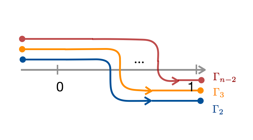
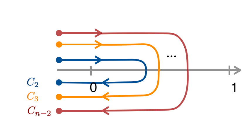
Figure 1: Integration contours associated with world-sheet variables $v_{i}^{-}$ in the KLT monodromy relations.

In this section we review a few details related to the string KLT monodromy relations that will become useful to our later derivations. It was demonstrated in BjerrumBohr:2010hn that when properly analytic continued, the world-sheet integral of a bosonic closed string amplitude factorises according to its dependence on light-cone coordinates $v_{i}^{\pm}=v_{i}^{1}\pm v_{i}^{2}$,

$$\mathcal{M}^{\rm closed}_{n}=\sum_{\alpha\in S_{n-3}}\mathcal{A}_{n}(1,\alpha,n-1,n)\,\mathcal{I}_{\alpha},$$ (4)

where the $v^{+}$ integrals together was identified as a colour-ordered bosonic open string amplitude $\mathcal{A}_{n}$, and the $v^{-}$ integrals together reads

$$\mathcal{I}_{23\dots n-2}=\int_{\Gamma_{2}}dv_{2}^{-}\int_{\Gamma_{3}}dv_{3}^{-}\dots\int_{\Gamma_{n-1}}dv_{n-1}^{-}\,\prod_{i=2}^{n-2}(v_{i}^{-})^{\alpha^{\prime}k_{1}\cdot k_{i}}(1-v_{i}^{-})^{\alpha^{\prime}k_{n-1}\cdot k_{i}}\prod_{i<j\leq n-2}(v_{i}^{-}-v_{j}^{-})^{\alpha^{\prime}k_{i}\cdot k_{j}}f(v_{i}^{-}),$$ (5)

where $f(v_{i}^{-})$ arises from the operator product expansion of the vertex operators. The integration contours $\Gamma_{2},\Gamma_{3},\dots,\Gamma_{n-2}$ illustrated in Fig 1 were defined to avoid branch cuts due to factors $(v_{i}^{-}-v_{j}^{-})^{\alpha^{\prime}k_{i}\cdot k_{j}}$, while variables $(v_{1}^{-},v_{n-1}^{-},v_{n}^{-})$ were gauge fixed by world-sheet Moebius invariance to be $(0,1,\infty)$ respectively. These contours were then pulled to the left, assuming no pole lying in the lower half plane. The result was to replace $\Gamma_{2}$, $\dots$, $\Gamma_{n-2}$ by a new set of contours defined along the branch cut $[0,-\infty)$ (Fig 1). It was noted that the phase difference between the two sides of the branch cut $[0,-\infty)$ in the $C_{2}$ integration produces an overall sine factor,

$$\int_{C_{2}}dv_{2}^{-}(v_{2})^{\alpha^{\prime}k_{1}\cdot k_{2}}(1-v_{2}^{-})^{\alpha^{\prime}k_{n-1}\cdot k_{2}}\prod_{j+3}^{n-2}(v_{j}^{-}-v_{2}^{-})^{\alpha^{\prime}k_{j}\cdot k_{2}}f(v_{2}^{-})$$

$$=2i\,\sin(\pi\alpha^{\prime}k_{1}\cdot k_{2})\int_{-\infty}^{0}dv_{2}^{-}(-v_{2}^{-})^{\alpha^{\prime}k_{1}\cdot k_{2}}(1-v_{2}^{-})^{\alpha^{\prime}k_{n-1}\cdot k_{2}}\prod_{j+3}^{n-2}(v_{j}^{-}-v_{2}^{-})^{\alpha^{\prime}k_{j}\cdot k_{2}}f(v_{2}^{-}).$$ (6)

and similarly for the contour $C_{3}$

$$\int_{C_{3}}dv_{3}^{-}(v_{3}^{-})^{\alpha^{\prime}k_{1}\cdot k_{3}}(1-v_{3}^{-})^{\alpha^{\prime}k_{n-1}\cdot k_{3}}(v_{3}^{-}-v_{2}^{-})^{\alpha^{\prime}k_{2}\cdot k_{3}}\prod_{j=4}^{n-2}(v_{j}^{-}-v_{3}^{-})^{\alpha^{\prime}k_{j}\cdot k_{3}}f(v_{3}^{-})$$

$$=2i\sin(\pi\alpha^{\prime}k_{1}\cdot k_{3})\int_{v_{2}^{-}}^{0}dv_{3}^{-}(-v_{3}^{-})^{\alpha^{\prime}k_{1}\cdot k_{3}}(1-v_{3}^{-})^{\alpha^{\prime}k_{n-1}\cdot k_{3}}(v_{3}^{-}-v_{2}^{-})^{\alpha^{\prime}k_{2}\cdot k_{3}}\prod_{j=4}^{n-2}(v_{j}^{-}-v_{3}^{-})^{\alpha^{\prime}k_{j}\cdot k_{3}}f(v_{3}^{-})$$

$$+2i\sin(\pi\alpha^{\prime}(k_{1}+k_{3})\cdot k_{3})\int_{-\infty}^{v_{2}^{-}}(-v_{3}^{-})^{\alpha^{\prime}k_{1}\cdot k_{3}}(1-v_{3}^{-})^{\alpha^{\prime}k_{n-1}\cdot k_{3}}(v_{2}^{-}-v_{3}^{-})^{\alpha^{\prime}k_{2}\cdot k_{3}}\prod_{j=4}^{n-2}(v_{j}^{-}-v_{3}^{-})^{\alpha^{\prime}k_{j}\cdot k_{3}}f(v_{3}^{-})\,.$$ (7)

Repeating the same manipulation on all contours led to the extraction of a momentum kernel, and the remaining factor was identified as another copy of the bosonic open string amplitude $\tilde{A}_{n}$,

$$\mathcal{I}_{23\dots n-1}=\sum_{\beta\in S_{n-3}}\mathcal{S}_{\alpha^{\prime}}[n-1,\dots,4,3,2|\beta]\,\tilde{\mathcal{A}}_{n}(n-1,n,\beta,1),$$ (8)

where the momentum kernel $\mathcal{S}_{\alpha^{\prime}}[i_{2},\dots,i_{k}|j_{2},\dots,j_{k}]_{p}$ in the context of string theory is defined as

$$\mathcal{S}_{\alpha^{\prime}}[i_{1},\dots,i_{k}|j_{1},\dots,j_{k}]_{p}:=(\pi\alpha^{\prime}/2)^{-k}\prod_{t=1}^{k}\sin(\pi\alpha^{\prime}(p\cdot k_{i_{t}}+\sum_{q>t}^{k}\theta(i_{t},i_{q})k_{i_{t}}\cdot k_{i_{q}})),$$ (9)

where $\theta(i_{t},i_{q})=1$ if the ordering of $i_{t}$ and $i_{q}$ is the opposite in the $\{i_{1},\dots,i_{k}\}$ and $\{j_{1},\dots,j_{k}\}$ and otherwise 0 if the ordering is the same. This expression becomes identical to the field theory momentum kernel BjerrumBohr:2010ta in the $\alpha^{\prime}\rightarrow 0$ limit

$$\mathcal{S}[i_{1},\dots,i_{k}|j_{1},\dots,j_{k}]_{p}=\prod_{t=1}^{k}(p\cdot k_{i_{t}}+\sum_{q>t}^{k}\theta(i_{t},i_{q})k_{i_{t}}\cdot k_{i_{q}}).$$ (10)

In the literature of colour-kinematics duality, it was realised that the momentum kernel relations described above offer a convenient solution to the kinematic numerators BjerrumBohr:2010zs ; Bern:2010yg . This is because if we treat the gravity amplitude as double copies and leave one copy of the Yang-Mills amplitude as it is, the other copy combines with the momentum kernel, which is understood to be the inverse of the propagator matrix, and produces an $(n-2)!$-basis half ladder numerator $n(1\alpha n)$ associated with that copy of the amplitude. The result is the familiar Del Duca-Dixon-Maltoni expression,

$$\mathcal{M}^{\rm closed}_{n}=\sum_{\alpha\in S_{n-2}}\mathcal{A}_{n}(1,\alpha,n)\,n(1\alpha n).$$ (11)

Comparing equation (11) with its string theory analogue (4), it is natural to conclude that the $v^{-}$ integral $\mathcal{I}_{\alpha}$ becomes the basis numerator $n(1\alpha n)$ in the $\alpha^{\prime}$ limit. One can express the half ladder numerator using the momentum kernel BjerrumBohr:2010hn as

$$n(1,\gamma(2),\gamma(3),\dots,\gamma(n-1),n)=\begin{cases}\sum_{\beta\in S_{n-3}}\mathcal{S}[\gamma^{T}|\beta]\,\tilde{\mathcal{A}}_{n}(1,\beta,n,n-1)&,\gamma(n-1)=n-1\\ 0&,\gamma(n-1)\neq n-1\,.\end{cases}$$ (12)

These numerators are not unique as any shifts proportional to the momentum kernel will not change the total amplitude (11). These numerators are not always local and can present poles Bern:2010yg but the total amplitude is always local. These non-localities are sometime useful in finding a colour-kinematics representation of gauge theory amplitudes Carrasco:2011mn , which is consistent with (8). The above prescription however has the apparent shortcoming that not all of its legs are treated on equal footing (which could be regarded as the result of a generalised gauge shift on the numerators) making it difficult to allow algebraic interpretation. It is also known that when applied to amplitudes that has an algebraic structure by construction such as those of the $\phi^{3}$ theory, an $(n-3)!$ minimal KLT basis (12) yields shifted numerators rather than the expected string of structure constant $f^{ab*}f^{*c*}f^{*d*}\dots$ . In view of these a slight modification to this approach was added in Mafra:2016ltu ; Du:2016tbc where the numerators were solved in a more symmetric $(n-2)!$ basis

$$n(1,\gamma(2),\gamma(3),\dots,\gamma(n-1),n)=\lim_{k_{n}^{2}\rightarrow 0}\sum_{\beta\in S_{n-2}}\frac{1}{k_{n}^{2}}\mathcal{S}[\gamma^{T}|\beta]\,\tilde{\mathcal{A}}_{n}(1,\beta,n)\,,$$ (13)

at the cost that one of the legs must be taken off-shell until the end of the calculation in order to keep a $(n-2)!$ basis momentum kernel matrix non-singular.

In the following sections we derive the kinematic algebra from string perspective using similar reasoning to that described above, except backwards. Starting with an $(n-2)!$ basis prescription for kinematic numerator (13), we translate the factors of sine introduced by momentum kernel as world-sheet integrals along two sides of a branch cut. (In light of the fact that an $(n-2)!$ basis prescription does lead to unshifted numerator for $\phi^{3}$ theory.) For this purpose an off-shell continuation to the string amplitude is introduced. As we shall see, the numerator thus defined does have a natural algebraic explanation.

3 An off-shell continuation of the open string amplitude

For the purpose of discussion we recall that an $n$-point bosonic open string amplitude is defined in the operator language as

$$\mathcal{A}_{n}=\alpha^{\prime n-3}g^{n-2}\Bigl{\langle}f\Bigr{|}V_{n-1}(1)\frac{1}{L_{0}-I}V_{n-2}(1)\dots V_{3}(1)\frac{1}{L_{0}-I}V_{2}(1)\Bigl{|}i\Bigr{\rangle}\,,$$ (14)

where the external states are $|f\rangle=\lim_{z_{n}\to\infty}z_{n}V(z_{n})|0\rangle$ and $|i\rangle=\lim_{z_{1}\to 0}z_{1}^{-1}V(z_{1})|0\rangle$ acting on the vacuum $|0\rangle$. In standard calculation Green:1987sp the propagators are replaced by integrals $\frac{1}{L_{0}-I}=\int_{0}^{1}dz\,z^{L_{0}-2}$, yielding

$$\mathcal{A}_{n} ={\alpha^{\prime}}^{n-3}\,g^{n-2}\,\int_{0}^{1}dz_{n-2}\dots\int_{0}^{1}dz_{3}\int_{0}^{1}dz_{2}\Bigl{\langle}f\Bigr{|}V_{n-1}(1)z_{n-2}^{L_{0}-2}V_{n-2}(1)z_{n-3}^{L_{0}-2}V_{n-3}(1)\dots z_{3}^{L_{0}-2}V_{3}(1)z_{2}^{L_{0}-2}V_{2}(1)\Bigl{|}i\Bigr{\rangle}$$

$$={\alpha^{\prime}}^{n-3}\,g^{n-2}\,\int_{0}^{1}\frac{dz_{n-2}}{z_{n-2}}\dots\int_{0}^{1}\frac{dz_{3}}{z_{3}}\int_{0}^{1}\frac{dz_{2}}{z_{2}}\Bigl{\langle}f\Bigr{|}V_{n-1}(1)\Bigl{(}z_{n-2}^{L_{0}-1}V_{n-2}(1)z_{n-2}^{-(L_{0}-1)}\Bigr{)}$$

$$\times\Bigl{(}(z_{n-2}z_{n-3})^{L_{0}-1}V_{n-1}(1)(z_{n-2}z_{n-3})^{-(L_{0}-1)}\Bigr{)}\dots\Bigl{(}(z_{3}z_{4}\dots z_{n-2})^{L_{0}-1}V_{3}(1)(z_{3}z_{4}\dots z_{n-2})^{-(L_{0}-1)}\Bigr{)}$$

$$\times\Bigl{(}(z_{2}z_{3}\dots z_{n-2})^{L_{0}-1}V_{2}(1)(z_{2}z_{3}\dots z_{n-2})^{-(L_{0}-1)}\Bigr{)}\Bigl{|}i\Bigr{\rangle}\,,$$ (15)

where in the second line above we simultaneously multiplied and divided by factors of $z_{i}^{L_{0}-1}$ between vertex operators. The familiar Veneziano type world-sheet integral formula is then obtained via a change of integration variables to

$$y_{2} :=z_{2}z_{3}z_{4}\dots z_{n-2}\,$$

$$y_{3} :=z_{3}z_{4}\dots z_{n-2}\,$$

$$\vdots$$

$$y_{n-2} :=z_{n-2}\,$$ (16)

and using the fact that vertex operators are primary fields of conformal dimension one, $V(y)=y^{L_{0}-1}V(1)y^{-(L_{0}-1)}$,

$$\mathcal{A}_{n}(123\dots n) =\alpha^{\prime n-3}g^{n-2}\int_{0<y_{2}<y_{3}<\dots<y_{n-2}<1}\prod_{i=2}^{n-2}dy_{i}\,\Bigl{\langle}f\Bigr{|}V_{n-1}(1)\,\frac{V_{n-2}(y_{n-2})}{y_{n-2}}\dots\frac{V_{3}(y_{3})}{y_{3}}\,\frac{V_{2}(y_{2})}{y_{2}}\Bigl{|}i\Bigr{\rangle}$$ (17)

$$=\alpha^{\prime n-3}g^{n-2}\int_{0<y_{2}<y_{3}<\dots<y_{n-2}<1}\prod_{i=2}^{n-2}dy_{i}\,y_{2}^{\alpha^{\prime}k_{2}\cdot k_{1}}(1-y_{2})^{\alpha^{\prime}k_{2}\cdot k_{n-1}}\prod_{i<j<n-2}(y_{j}-y_{i})^{\alpha^{\prime}k_{j}\cdot k_{i}}f(y_{i}),$$

where $f(y_{i})$ arises from the operator product expansion of the vertex operators. The integration domain changes as a result to $0<y_{2}<y_{3}<\dots<y_{n-2}<1$.

Instead of equation (14), we consider a similar formula ended however with an off-shell final state,

$$\mathcal{J}_{n}(123\dots n) :=\alpha^{\prime n-3}g^{n-2}\frac{1}{\hat{k}_{n}^{2}}\Bigl{\langle}\hat{f}\Bigr{|}V_{n-1}(1)\frac{1}{L_{0}-I}V_{n-2}(1)\dots\frac{1}{L_{0}-I}V_{2}(1)\Bigl{|}\hat{i}\Bigr{\rangle}$$

$$=\alpha^{\prime n-2}g^{n-2}\Bigl{\langle}\hat{f}\Bigr{|}\frac{1}{L_{0}-I}V_{n-1}(1)\frac{1}{L_{0}-I}V_{n-2}(1)\dots\frac{1}{L_{0}-I}V_{2}(1)\Bigl{|}\hat{i}\Bigr{\rangle}.$$ (18)

where the off-shell continuation is defined through BCFW-like shifting $\hat{k}_{n}=k_{n}+\epsilon q$ and $\hat{k}_{1}=k_{1}-\epsilon q$, with the shifting chosen such that $q\cdot k_{1}=0$ while $q\cdot k_{n}\neq 0$, and the initial and final states are defined as

$$\Bigl{|}\hat{i}\Bigr{\rangle} :=\epsilon_{1}\cdot\alpha_{-1}e^{i(k_{1}-\epsilon q)\cdot x}\Bigl{|}0\Bigr{\rangle}\,$$ (19)

$$\Bigl{|}\hat{f}\Bigr{\rangle} :=\epsilon_{n}\cdot\alpha_{-1}e^{i(k_{n}+\epsilon q)\cdot x}\Bigl{|}0\Bigr{\rangle}\,.$$

The same off-shell continuation was introduced earlier in field theory amplitudes in Feng:2010hd to define KLT monodromy relations in an $(n-2)!$ basis. Note that this is different from how the off-shell continuation would usually be defined on string amplitudes offshell-string1 ; Liccardo:1999hk , since conformal symmetry is respected by vertex operators only when on-shell, and it makes little sense to define a vertex operator if we are not allowed to shrink the external leg to a point via conformal transformation in the first place. Nevertheless, it is apparent that apart from an overall $1/k_{n}^{2}$, equation (18) formally agrees with the amplitude (14) in the on-shell limit. In this sense equation (18) is a string analogue of the off-shell current. As in the standard amplitude calculation discussed above we then replace all propagators, including the newly introduced one by the off-shell leg, and write

$$\mathcal{J}_{n}(123\dots n)=\alpha^{\prime n-3}g^{n-2}\int_{0}^{1}\frac{dz_{n-1}}{z_{n-1}}\dots\int_{0}^{1}\frac{dz_{3}}{z_{3}}\int_{0}^{1}\frac{dz_{2}}{z_{2}}\Bigl{\langle}\hat{f}\Bigr{|}\Bigl{(}z_{n-1}^{L_{0}-1}V_{n-1}(1)z_{n-1}^{-(L_{0}-1)}\Bigr{)}\cr\Bigl{(}(z_{n-1}z_{n-2})^{L_{0}-1}V_{n-1}(1)(z_{n-1}z_{n-2})^{-(L_{0}-1)}\Bigr{)}\dots\Bigl{(}(z_{3}z_{4}\dots z_{n-1})^{L_{0}-1}V_{3}(1)(z_{3}z_{4}\dots z_{n-1})^{-(L_{0}-1)}\Bigr{)}\cr\times\Bigl{(}(z_{2}z_{3}\dots z_{n-1})^{L_{0}-1}V_{2}(1)(z_{2}z_{3}\dots z_{n-1})^{-(L_{0}-1)}\Bigr{)}\Bigl{|}\hat{i}\Bigr{\rangle}\,.$$ (20)

A similar change of variables

$$y_{2} :=z_{2}z_{3}z_{4}\dots z_{n-1}\,$$

$$y_{3} :=z_{3}z_{4}\dots z_{n-1}\,$$

$$\vdots$$

$$y_{n-2} :=z_{n-2}z_{n-1}\,$$

$$y_{n-1} :=z_{n-1}\,,$$ (21)

this time leads to $(n-2)$ instead of $(n-3)$ vertex operators to be integrated between $(0,1)$,

$$\mathcal{J}_{n}(123\dots n)=(\alpha^{\prime}g)^{n-2}\int_{0<y_{2}<y_{3}<\dots<y_{n-1}<1}\prod_{i=2}^{n-2}dy_{i}\,\Bigl{\langle}\hat{f}\Bigr{|}\frac{V_{n-1}(y_{n-1})}{y_{n-1}}\,\frac{V_{n-2}(y_{n-2})}{y_{n-2}}\dots\frac{V_{3}(y_{3})}{y_{3}}\,\frac{V_{2}(y_{2})}{y_{2}}\Bigl{|}\hat{i}\Bigr{\rangle}.$$ (22)

As discussed earlier in this paper, in light of the fact that field theory momentum kernel happens to be the inverse of propagator matrix in an$(n-2)!$ basis, the (field theory) numerator can be calculated from the $\alpha^{\prime}$ limit of the following sum over $(n-2)!$ permutations of the legs $\{2,3,4,\dots,n-1\}$,

$$n(123\dots n)=\lim_{k_{n}^{2},\alpha^{\prime}\rightarrow 0}\,\sum_{\beta\in S_{n-2}}\mathcal{S}_{\alpha^{\prime}}[n-1,\dots,4,3,2|\beta]\,\mathcal{J}_{n}(1,\beta,n).$$ (23)

Despite perhaps a bit complicated at first sight, it is known Du:2011js ; Du:2016tbc that the above permutation sum very often simplifies if we organise the amplitudes (or currents) in the equation according to the so-called Fundamental BCJ relations BjerrumBohr:2009rd ; Stieberger:2009hq ; Feng:2010my ,

$$n(123\dots n)= \lim_{k_{n}^{2},\alpha^{\prime}\rightarrow 0}\,\sum_{\beta\in S_{n-3}}\mathcal{S}_{\alpha^{\prime}}[n-2,\dots,4,3,2|\beta]\,\Bigl{\{}2i\sin(\pi\alpha^{\prime}k_{n-1}\cdot k_{1})\mathcal{J}_{n}(1,n-1,\beta_{2},\beta_{3},\dots,\beta_{n-2},n)$$

$$+2i\sin(\pi\alpha^{\prime}k_{n-1}\cdot(k_{1}+k_{\beta_{2}}))\mathcal{J}_{n}(1,\beta_{2},n-1,\beta_{3},\dots,\beta_{n-2},n)$$

$$+\dots$$

$$+2i\sin(\pi\alpha^{\prime}k_{n-1}\cdot(k_{1}+k_{\beta_{2}}+\dots+k_{\beta_{n-2}}))\mathcal{J}_{n}(1,\beta_{2},\beta_{3},\dots,\beta_{n-2},n-1,n)\Bigr{\}}.$$ (24)

Explicitly we focus first on the subset of the full $(n-2)!$ permutation sum in equation (23) where leg $(n-1)$ is inserted between the relatively fixed set $\{2,3,4,\dots,n-2\}$. It is straightforward to see from the definition of momentum kernel that this is proportional to

$$2i\sin(\pi\alpha^{\prime}k_{n-1}\cdot k_{1})\mathcal{J}_{n}(1,n-1,2,3,\dots,n-2,n)+2i\sin(\pi\alpha^{\prime}k_{n-1}\cdot(k_{1}+k_{2}))\mathcal{J}_{n}(1,2,n-1,3,\dots,n-2,n)$$

$$+\dots+2i\sin(\pi\alpha^{\prime}k_{n-1}\cdot(k_{1}+k_{2}+\dots+k_{n-2}))\mathcal{J}_{n}(1,2,3,\dots,n-2,n-1,n)\,.$$ (25)

To complete this calculation we then perform an $(n-3)!$ permutation sum on the originally fixed set $\{2,3,4,\dots,n-2\}$, which in turn can be organised into BCJ sums if we regard it as insertions of the leg $(n-2)$ between set $\{2,3,4,\dots,n-3\}$ and so on. We will see in the next section that algebraic structure can be identified in this process. We shall also drop the distinction between $\Bigl{|}\hat{f}\Bigr{\rangle}$ and $\Bigl{|}f\Bigr{\rangle}$ since it is known that at least in the field theory limit, numerators obtained through equation (13) remain finite in the on-shell limit.

4 Half-ladder basis numerators and the vertex operator algebra

The BCJ sum (25) written down in the last section can be more easily understood in the language of vertex operators. We will in the following illustrate this idea through two lower-point examples. For simplicity we will assume the scattering particles are all tachyons, although the generalisation to gluons is straightforward.

4.1 The three point numerator

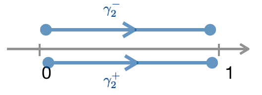
Figure 2: Integration contours present in the evaluation of three point kinematic numerator

Consider the numerator at three points. Equation (23) reads

$$2i\,\sin(\pi\alpha^{\prime}k_{2}\cdot k_{1})g\alpha^{\prime}\int_{0}^{1}\frac{dy_{2}}{y_{2}}\,y_{2}^{\alpha^{\prime}k_{2}\cdot k_{1}}=g\alpha^{\prime}\int_{\gamma_{2}^{+}-\gamma_{2}^{-}}\frac{dy_{2}}{y_{2}}\,\left(-y_{2}\right)^{\alpha^{\prime}k_{2}\cdot k_{1}}\,,$$ (26)

where we followed the same reasoning used in the extraction of string momentum kernel from monodromy relations BjerrumBohr:2010hn to translate the sine factor into the difference between integrals $\gamma_{2}^{+}$ and $\gamma_{2}^{-}$ along opposite sides of a branch cut (Fig 2). To see how equation (26) can have an algebraic origin, recall that in the operator language a Veneziano type world-sheet integral formula derives from normal ordering two vertex operators

$$V(y_{1})V(y_{2}) =\left(e^{\sqrt{\alpha^{\prime}}\sum_{1}^{\infty}\frac{k_{1}\cdot\alpha_{-n}}{n}y_{1}^{n}}e^{-\sqrt{\alpha^{\prime}}\sum_{1}^{\infty}\frac{k_{1}\cdot\alpha_{n}}{n}y_{1}^{-n}}e^{ik_{1}\cdot x}e^{k_{1}\cdot p\,\ln y_{1}}\right)$$ (27)

$$\times\left(e^{\sqrt{\alpha^{\prime}}\sum_{1}^{\infty}\frac{k_{2}\cdot\alpha_{-n}}{n}y_{2}^{n}}e^{-\sqrt{\alpha^{\prime}}\sum_{1}^{\infty}\frac{k_{2}\cdot\alpha_{n}}{n}y_{2}^{-n}}e^{ik_{2}\cdot x}e^{k_{2}\cdot p\,\ln y_{2}}\right)$$

$$=e^{\alpha^{\prime}k_{1}\cdot k_{2}\,\ln y_{1}}e^{-\alpha^{\prime}\sum_{1}^{\infty}\frac{1}{n}\left(\frac{y_{2}}{y_{1}}\right)^{n}}:V(y_{1})V(y_{2}):$$

$$\sim e^{\alpha^{\prime}k_{1}\cdot k_{2}\,\ln(y_{1}-y_{2})}f(y).$$ (28)

Starting from a point $y_{2}$ on the real line with $\Bigl{|}\frac{y_{2}}{y_{1}}\Bigr{|}<1$ so that the infinite series converges $-\sum_{1}^{\infty}\frac{1}{n}\left(\frac{y_{2}}{y_{1}}\right)^{n}=\ln(1-\frac{y_{2}}{y_{1}})$, the analytic continuation of the product $V(y_{1})V(y_{2})\sim e^{\alpha^{\prime}k_{1}\cdot k_{2}\,\ln(y_{1}-y_{2})}f(y)$ is uniquely determined as $y_{2}$ travels continuously on the complex plane. Bearing this in mind, it is straightforward to see that integration contour associated with the ordered product

$$\frac{V(y_{1})}{y_{1}}\,\left(\int_{0}^{1}dy_{2}\frac{V(y_{2})}{y_{2}}\right)\,,$$ (29)

analytically continues as illustrated in Fig 3(a), while the contour associated with opposite order

$$\left(\int_{0}^{1}dy_{2}\frac{V(y_{2})}{y_{2}}\right)\,\frac{V(y_{1})}{y_{1}}\,,$$ (30)

corresponds to Fig 3(b). (In the later case $V(y_{2})V(y_{1})\sim e^{\alpha^{\prime}k_{1}\cdot k_{2}\,\ln(y_{2}-y_{1})}f(y)$ and the branch cut lies along the $y_{2}<y_{1}$ part of the real line.)

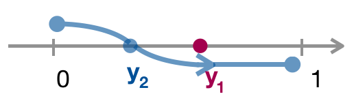
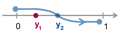
Figure 3: The contours corresponding to $V_{1}V_{2}$ and $V_{2}V_{1}$ respectively.

A careful inspection on the three-point numerator obtained earlier in (26) then shows that the numerator can be written in the operator language as

$$\alpha^{\prime}\int_{\gamma_{2}^{+}}\frac{dy_{2}}{y_{2}}\,\left(-y_{2}\right)^{\alpha^{\prime}k_{2}\cdot k_{1}}-e^{-i\pi\alpha^{\prime}k_{2}\cdot k_{1}}\alpha^{\prime}\int_{\gamma_{2}^{-}}\frac{dy_{2}}{y_{2}}\,y_{2}^{\alpha^{\prime}k_{2}\cdot k_{1}}$$

$$=\alpha^{\prime}\left(\int_{0}^{1}dy_{2}\Bigl{\langle}f\Bigr{|}\frac{V_{1}(y_{1})}{y_{1}}\,\frac{V_{2}(y_{2})}{y_{2}}\Bigl{|}0\Bigr{\rangle}-e^{-i\pi\alpha^{\prime}k_{2}\cdot k_{1}}\int_{0}^{1}dy_{2}\Bigl{\langle}f\Bigr{|}\frac{V_{2}(y_{2})}{y_{2}}\,\frac{V_{1}(y_{1})}{y_{1}}\Bigl{|}0\Bigr{\rangle}\right)\Bigr{|}_{y_{1}\rightarrow 0}$$

$$=\alpha^{\prime}\Bigl{\langle}f\Bigr{|}[T_{1},T_{2}]_{\alpha^{\prime}}\Bigl{|}0\Bigr{\rangle}\,,$$ (31)

where $\langle f|$ is the external state defined (19) for $n=3$. This is in some sense the structure we anticipated. However instead of a Lie bracket, we arrive at a similar, yet asymmetric structure defined as

$$[T_{1},T_{2}]_{\alpha^{\prime}}=T_{1}T_{2}-e^{-i\pi\alpha^{\prime}k_{2}\cdot k_{1}}T_{2}T_{1}$$ (33)

where we introduced the shorthand notation to denote $T_{2}=\int_{0}^{1}dy_{2}\frac{V_{2}(y_{2})}{y_{2}}$ and $T_{1}=\frac{V_{1}(y_{1})}{y_{1}}\Bigr{|}_{y_{1}\rightarrow 0}$.

4.2 Four points and higher

The numerator at four points follows similar calculations. As discussed earlier we note that BCJ sums can be extracted from the full $(n-2)!$ permutation sum appears in (23).

$$2i\,\sin(\pi\alpha^{\prime}k_{3}\cdot k_{1})\mathcal{J}_{4}(1324)+2i\,\sin(\pi\alpha^{\prime}k_{3}\cdot(k_{1}+k_{2}))\mathcal{J}_{4}(1234)$$

$$=2i\,\sin(\pi\alpha^{\prime}k_{3}\cdot k_{1})g^{2}{\alpha^{\prime}}^{2}\int_{0}^{y_{2}}\frac{dy_{3}}{y_{3}}\,y_{3}^{\alpha^{\prime}k_{3}\cdot k_{1}}(y_{2}-y_{3})^{\alpha^{\prime}k_{3}\cdot k_{2}}f(y_{3})$$

$$+2i\,\sin(\pi\alpha^{\prime}k_{3}\cdot(k_{1}+k_{2}))g^{2}{\alpha^{\prime}}^{2}\int_{y_{2}}^{1}\frac{dy_{3}}{y_{3}}\,y_{3}^{\alpha^{\prime}k_{3}\cdot k_{1}}(y_{3}-y_{2})^{\alpha^{\prime}k_{3}\cdot k_{2}}f(y_{3})$$

$$=g^{2}{\alpha^{\prime}}^{2}\int_{\gamma_{3}^{+}-\gamma_{3}^{-}}\frac{dy_{3}}{y_{3}}\,\left(-y_{3}\right)^{\alpha^{\prime}k_{3}\cdot k_{1}}(y_{2}-y_{3})^{\alpha^{\prime}k_{3}\cdot k_{2}}f(y_{3})\,,$$ (34)

where in the last line of the equation above we translated the phase factors introduced by sines into the difference between integrals $\gamma_{3}^{+}$ and $\gamma_{3}^{-}$ below and above the branch cut, similar to those illustrated in Fig 2. The first and the second term contribute the $0<\Bigl{|}y_{3}\Bigr{|}<y_{2}$ and $y_{2}<\Bigl{|}y_{3}\Bigr{|}<1$ segment of the $\gamma_{3}^{+}$ contour respectively, and likewise for the contour $\gamma_{3}^{-}$. The integration in equation (34) can be subsequently rewritten as

$$\int_{\gamma_{3}^{+}}\frac{dy_{3}}{y_{3}}\,\left(-y_{3}\right)^{\alpha^{\prime}k_{3}\cdot k_{1}}(y_{2}-y_{3})^{\alpha^{\prime}k_{3}\cdot k_{2}}f(y_{3})-e^{i\pi\alpha^{\prime}k_{3}\cdot(k_{1}+k_{2})}\int_{\gamma_{3}^{-}}\frac{dy_{3}}{y_{3}}\,y_{3}^{\alpha^{\prime}k_{3}\cdot k_{1}}(y_{3}-y_{2})^{\alpha^{\prime}k_{3}\cdot k_{2}}f(y_{3})$$

$$=\Bigl{\langle}f\Bigr{|}\frac{V(y_{2})}{y_{2}}\,\frac{V(y_{1})}{y_{1}}\,\left(\int_{0}^{1}dy_{3}\frac{V(y_{3})}{y_{3}}\right)\Bigl{|}0\Bigr{\rangle}-e^{i\pi\alpha^{\prime}k_{3}\cdot(k_{1}+k_{2})}\Bigl{\langle}f\Bigr{|}\left(\int_{0}^{1}dy_{3}\frac{V(y_{3})}{y_{3}}\right)\,\frac{V(y_{2})}{y_{2}}\,\frac{V(y_{1})}{y_{1}}\Bigl{|}0\Bigr{\rangle}\,,$$ (35)

again here $\langle f|$ is the external state defined (19) for $n=4$. What remains in the calculation is a multiplication by $2i\,\sin(\pi\alpha^{\prime}k_{2}\cdot k_{1})$, which has the same effect as was shown at three points, and we arrive at

$$n(1234)=g^{2}{\alpha^{\prime}}^{2}\lim_{k_{4}^{2},\alpha^{\prime}\rightarrow 0}\Bigl{\langle}f\Bigr{|}[[T_{1},T_{2}]_{\alpha^{\prime}},T_{3}]_{\alpha^{\prime}}\Bigl{|}0\Bigr{\rangle}\,,$$ (36)

where $T_{2}=\int_{0}^{1}dy_{2}\frac{V_{2}(y_{2})}{y_{2}}$, $T_{3}=\int_{0}^{1}dy_{3}\frac{V_{3}(y_{3})}{y_{3}}$ and $T_{1}=\frac{V_{1}(y_{1})}{y_{1}}\Bigr{|}_{y_{1}\rightarrow 0}$. Generically this translation procedure continues, and the $n$-point half-ladder basis numerator is given by

$$n(123\dots n)=g^{n-2}{\alpha^{\prime}}^{n-2}\lim_{k_{n}^{2},\alpha^{\prime}\rightarrow 0}\Bigl{\langle}f\Bigr{|}[[[T_{1},T_{2}]_{\alpha^{\prime}},T_{3}]_{\alpha^{\prime}}\dots,T_{n-1}]_{\alpha^{\prime}}\Bigl{|}0\Bigr{\rangle}.$$ (37)

Incidentally the same $\alpha^{\prime}$-weighted commutator structure was actually observed earlier in Ma:2011um from a rather different perspective, and more recently in Carrasco:2016ygv . There it was shown that, starting from the standard colour-order formulation and applying the Kleiss-Kuijf relations Kleiss:1988ne on the colour-ordered open string amplitudes, the result is a formula bearing much resemblance to the Del Duca-Dixon-Maltoni expression, except with the Lie bracket between the $SU(N)$ colour generators $t_{a}$ replaced by exactly the same $\alpha^{\prime}$-weighted commutator (33).

$$\mathcal{M}_{n} =\sum_{\rho\in S_{n-1}}tr(t_{\rho(1)}t_{\rho(2)}\dots t_{\rho(n-1)}t_{n})\,\mathcal{A}_{n}(\rho(1),\rho(2),\dots,\rho(n-1),n)$$

$$=\sum_{\sigma\in S_{n-2}}tr([[[t_{1},t_{\sigma(2)}]_{\alpha^{\prime}},t_{\sigma(3)}]_{\alpha^{\prime}}\dots,t_{\sigma(n-1)}]_{\alpha^{\prime}}t_{n})\,\mathcal{A}_{n}(1,\sigma(2),\dots,\sigma(n-1),n)\,.$$ (38)

In this sense we see that the numerator structure (37) just derived serves as the colour-kinematics counterpart of (38) in the context of string theory.

Note that the asymmetry feature of the new bracket $[\,,\,]_{\alpha^{\prime}}$ is entirely introduced by the phase factor $e^{-i\pi\alpha^{\prime}k_{1}\cdot k_{2}}$ which vanishes in the $\alpha^{\prime}\rightarrow 0$ limit, so that as far as field theory is concerned, we might as well replace all bracket with Lie bracket in the (field theory) numerator formula. In the section 4.3 we will work out some explicit examples. The basis numerator $n(123\dots n)$ thus obtained apparently respects Jacobi identity. Under this setting, a generic (not necessarily half-ladder) numerator is then simply given by the commutator structure suggested by its associated cubic graph, for example

$$\begin{minipage}{119.50148pt} \includegraphics[width=119.50148pt]{tree} \end{minipage}\sim[[T_{1},T_{2}],[T_{3},T_{4}]]$$ (39)

4.3 Explicit generators

Despite the apparent formal simplicity attained by expressing kinematic numerator in the language of vertex operator algebra, it is not yet clear to us whether the generator $T_{i}=\int_{0}^{1}dy\frac{V_{i}(y)}{y}$ has a simple representation so that the numerators can be calculated from the algebra directly. Instead, in this section we carry out the integral term-wise. Hopefully the calculation can provide useful insight regarding the analytic behaviour of the generators.

As an illustration of how this proceeds, for the moment we make a bit of digression and calculate the three-point numerator directly instead of calculating $T_{i}$, which takes the same generic form as far as the integral is concerned, except simpler. The four-point case requires the evaluation of the disc integral and will be treated in section 5.3. Taking into account that momentum kernel at three points is simply a sine factor, and that the current is given by equation (22), the numerator defined in (23) reads

$$n(123)=\lim_{k_{3}^{2},\alpha^{\prime}\rightarrow 0}\sin(\pi\alpha^{\prime}k_{2}\cdot k_{1})g\alpha^{\prime}\Bigl{\langle}\tilde{f}\Bigr{|}:\int_{0}^{1}\frac{dy_{2}}{y_{2}}\epsilon_{2}\cdot X(y_{2})e^{ik_{2}\cdot X}:\,\Bigl{|}\tilde{i}\Bigr{\rangle}.$$ (40)

Plugging the explicit mode expansion of the vertex operator shows that the expectation value contributes the following integral.

$$\Bigl{\langle}\tilde{f}\Bigr{|}:\int_{0}^{1}\frac{dy_{2}}{y_{2}}\epsilon_{2}\cdot X(y_{2})e^{ik_{2}\cdot X}:\,\Bigl{|}\tilde{i}\Bigr{\rangle}=V_{3}\,\int_{0}^{1}dy_{2}\frac{1}{y_{2}}e^{\alpha^{\prime}k_{2}\cdot k_{1}\,\ln y_{2}}\,,$$ (41)

where $V_{3}$ is the Yang-Mills cubic

$$V_{3}=\left(\epsilon_{2}\cdot\epsilon_{1}\right)\left(k_{2}\cdot\epsilon_{3}\right)+\left(\epsilon_{3}\cdot\epsilon_{2}\right)\left(k_{2}\cdot\epsilon_{1}\right)+\left(\epsilon_{3}\cdot\epsilon_{1}\right)\left(k_{2}\cdot\epsilon_{1}\right)\,.$$ (42)

Namely in this case the world-sheet integral factorises, and gives

$$\int_{0}^{1}dy_{2}\,\left(y_{2}\right)^{\alpha^{\prime}k_{2}\cdot k_{1}-1}=\frac{1}{\alpha^{\prime}k_{2}\cdot k_{1}}\,.$$ (43)

The three-point current is therefore $V_{3}/k_{3}^{2}$ as expected. Multiplying current by momentum kernel $\sin(\pi\alpha^{\prime}k_{2}\cdot k_{1})\sim\pi\alpha^{\prime}k_{2}\cdot k_{1}$ shows that the numerator is $V_{3}$ in the $\alpha^{\prime}$ limit, which is consistent with known result.

The integral involved in calculating the $T_{a}$’s is similar. Assuming vertex operator has the following expansion,

$$V(y)=\sum_{n=-\infty}^{\infty}e^{ik\cdot x}a_{n}y^{n}e^{\sqrt{\alpha^{\prime}}k\cdot p\,\ln\,y}\,,$$ (44)

where $a_{n}$ are expansion coefficients, the integration of interest $\int_{0}^{1}dy\frac{V(y)}{y}$ can be readily carried out term-wise.

$$\int_{0}^{1}\frac{dy}{y}V(y) =\sum_{n=-\infty}^{\infty}e^{ik\cdot x}a_{n}\frac{1}{\sqrt{\alpha^{\prime}}k\cdot\alpha_{0}+n}\,.$$ (45)

The expansion coefficients $a_{n}$ are not so difficult to compute either. Keeping only the first few power terms in $\sqrt{\alpha^{\prime}}$, we have

$$a_{0}= \dots+\epsilon\cdot\alpha_{1}\left(\sqrt{\alpha^{\prime}}k\cdot\alpha_{-1}-\sqrt{\alpha^{\prime}}^{2}\sum_{n=1}^{\infty}\left(\frac{k\cdot\alpha_{-(n+1)}}{n+1}\right)\left(\frac{k\cdot\alpha_{n}}{n}\right)+\mathcal{O}(\sqrt{\alpha^{\prime}}^{3})\right)$$

$$+\epsilon\cdot\alpha_{0}\left(1-\sqrt{\alpha^{\prime}}^{2}\sum_{n=1}^{\infty}\left(\frac{k\cdot\alpha_{-n}}{n}\right)\left(\frac{k\cdot\alpha_{n}}{n}\right)+\mathcal{O}(\sqrt{\alpha^{\prime}}^{3})\right)$$

$$+\epsilon\cdot\alpha_{-1}\left(-\sqrt{\alpha^{\prime}}k\cdot\alpha_{1}-\sqrt{\alpha^{\prime}}^{2}\sum_{n=1}^{\infty}\left(\frac{k\cdot\alpha_{-n}}{n}\right)\left(\frac{k\cdot\alpha_{n+1}}{n+1}\right)+\mathcal{O}(\sqrt{\alpha^{\prime}}^{3})\right)+\dots\,,$$ (46)

and similarly for the rest of the $a_{n}$.

5 Structure constants of the vertex operator algebra

In light of the vertex operator expression of the BCJ numerators, a natural question to ask is whether the algebraic structure observed can be identified with any existing algebra. Note especially in Green:1987sp this was done in a similar setting to explain the $E_{8}\times E_{8}$ symmetry of the heterotic string theory, in which case all momentum inner product $k_{i}\cdot k_{j}$ appear in the exponent take integer values due to the compactification so that the world-sheet integrals can be elegantly performed. In the presence of branch cuts the story gets considerably messier. We saw in the last section that the generators can be calculated in a term-by-term basis, in this sense it is part of the universal enveloping algebra $U(g)$ of Virasoro modes, which is however too general to provide any useful information. On the other hand it is known that the self-dual sector of Yang-Mills numerator is explained by area-preserving diffeomorphism algebra as exploited in Monteiro:2011pc . We shall see in the following discussion that in the field theory limit, the vector $\times$ vector $\rightarrow$ vector sector is indeed isomorphic to diffeomorphism. We will see that the $\alpha^{\prime}$-weighted commutator (33) produces the familiar structure constant

$$f_{ab}{}^{c}=-i\left(\delta_{a}{}^{c}k_{1b}-\delta_{b}{}^{c}k_{2a}\right)\,,$$ (47)

up to $\alpha^{\prime}$ corrections.

5.1 Reproducing the diffeomorphism algebra

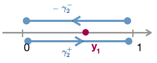
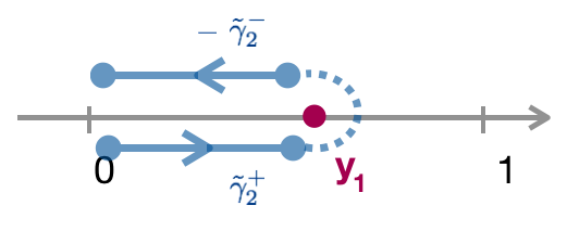
Figure 4: The contours present in the $\alpha^{\prime}$-weighted commutator calculation

For simplicity we write the vertex operator for vector particle as $V(y)=e^{ik\cdot X+\epsilon\cdot\dot{X}}$, bearing in mind that all calculations in the following are kept only to the first order in $\epsilon_{i}$’s. It is then straightforward to compute the product of two vertex operators using standard Wick contractions. Recall that the integration contours associated with the products $V_{1}(y_{1})V_{2}(y_{2})$ and $V_{2}(y_{2})V_{1}(y_{1})$ correspond to Fig 3(a) and (b) respectively. Taking a relative minus sign and phase into account, we see that the $\alpha^{\prime}$-weighted commutator is given by the following formula, integrated over the contour $\gamma^{+}-\gamma^{-}$shown in Fig 4, or equivalently, over the arc surrounding $y_{1}$ plus the difference $\tilde{\gamma}_{2}^{+}-\tilde{\gamma}_{2}^{-}$ along two sides of the branch cut $(0,y_{1})$ (Fig 4).

$$\int_{0}^{1}\frac{dy_{2}}{y_{2}}[V_{1}(y_{1}),V_{2}(y_{2})]_{\alpha^{\prime}}= \int_{\text{around }y_{1}}+\int_{\tilde{\gamma}^{+}-\tilde{\gamma}^{-}}\frac{dy_{2}}{y_{2}}\,e^{\alpha^{\prime}k_{1}\cdot k_{2}\ln(y_{1}-y_{2})}$$

$$\left(1-\alpha^{\prime}\epsilon_{2}\cdot k_{1}\frac{y_{2}}{y_{1}-y_{2}}+\alpha^{\prime}\epsilon_{1}\cdot k_{2}\frac{y_{1}}{y_{1}-y_{2}}+\alpha^{\prime}\epsilon_{1}\cdot\epsilon_{2}\frac{y_{1}y_{2}}{(y_{1}-y_{2})^{2}}\right.$$

$$\left.-\alpha^{\prime 2}(\epsilon_{1}\cdot k_{2})(\epsilon_{2}\cdot k_{1})\frac{y_{1}y_{2}}{(y_{1}-y_{2})^{2}}\right):V_{1}(y_{1})V_{2}(y_{2}):\Bigr{|}_{\text{linear in }\epsilon}\,.$$ (48)

The $\epsilon_{1}\cdot\epsilon_{2}$ term can be made to vanish with suitable gauge choice or for a self-dual Yang-Mills amplitude, therefore we know that it is not relevant to the structure of interest here; while the $(\epsilon_{1}\cdot k_{2})(\epsilon_{2}\cdot k_{1})$ term carries an $\alpha^{\prime 2}$ and becomes sub-leading in the field theory limit. We have checked that the construction generalises to the superstring in similar fashion as the supersymmetric Berends-Giele current of (Berg:2016fui, , App. A). For the moment let us focus first on the $\epsilon_{1}\cdot k_{2}$ and $\epsilon_{2}\cdot k_{1}$ terms. We will soon see that these two terms reproduce the familiar diffeomorphism structure constant multiplied by a vector (spin 1) vertex operator, whereas the factor $1$ contributes the tensor part and the $\epsilon_{1}\cdot\epsilon_{2}$ a scalar (spin 0) needed to reproduce the quartic vertex contribution in the field theory limit.

For generic values of $k_{1}\cdot k_{2}$ the integral around $y_{1}$ vanishes as the radius of the arc $\varepsilon$ approaches zero. This is because the normal ordered product $:V_{1}(y_{1})V_{2}(y_{2}):$ contains no pole at $y_{1}$ so that when expanded as power series of $(y_{2}-y_{1})$, the integral becomes

$$\int_{-\pi}^{\pi}\varepsilon e^{i\theta}id\theta\frac{1}{\varepsilon e^{i\theta}}\,e^{\alpha^{\prime}k_{1}\cdot k_{2}(\ln\varepsilon+i\theta)}\Bigl{(}c_{0}+c_{1}\varepsilon e^{i\theta}+\dots\Bigr{)}\xrightarrow{\varepsilon\rightarrow 0}\,0\,.$$ (49)

Similarly, we consider formally expanding $:V_{1}(y_{1})V_{2}(y_{2}):$ in the $\tilde{\gamma}^{+}$ and $\tilde{\gamma}^{-}$ part of the integral, and note that an $n$-th power term contributes as

$$\int_{\tilde{\gamma}_{2}^{\pm}}dy_{2}(y_{2}-y_{1})^{n}\,e^{\alpha^{\prime}k_{1}\cdot k_{2}\ln(y_{1}-y_{2})} =e^{i\pi\alpha^{\prime}k_{1}\cdot k_{2}}\int_{0\mp i\varepsilon}^{y_{1}\mp i\varepsilon}dy_{2}(y_{2}-y_{1})^{n+\alpha^{\prime}k_{1}\cdot k_{2}}$$

$$=\frac{1}{n+\alpha^{\prime}k_{1}\cdot k_{2}+1}e^{i\pi\alpha^{\prime}k_{1}\cdot k_{2}}\left[0-e^{\mp i\pi\alpha^{\prime}k_{1}\cdot k_{2}}e^{\alpha^{\prime}k_{1}\cdot k_{2}\ln\,y_{1}}\right].$$

For generic integer $n$ the difference $\tilde{\gamma}_{2}^{+}-\tilde{\gamma}_{2}^{-}$ then yields $\frac{2i\,\sin(\pi\alpha^{\prime}k_{1}\cdot k_{2})}{n+\alpha^{\prime}k_{1}\cdot k_{2}+1}e^{\alpha^{\prime}k_{1}\cdot k_{2}\ln\,y_{1}}$, which also vanishes as $\alpha^{\prime}\rightarrow 0$. The only exception occurs when $n=-1$, in which case the difference $\tilde{\gamma}_{2}^{+}-\tilde{\gamma}_{2}^{-}$ returns a finite result,

$$\frac{2i\,\sin(\pi\alpha^{\prime}k_{1}\cdot k_{2})}{\alpha^{\prime}k_{1}\cdot k_{2}}e^{\alpha^{\prime}k_{1}\cdot k_{2}\ln\,y_{1}}=2\pi i+\mathcal{O}(\alpha^{\prime}).$$ (50)

In other words the effect of the branch cut integration and the $\alpha^{\prime}$ limit combine is equivalent to stripping off an exponential phase factor $e^{\alpha^{\prime}k_{1}\cdot k_{2}\ln(y_{1}-y_{2})}$ and picking up the $-1$ power term coefficient if we imagine the rest of the integrand $\left(-\alpha^{\prime}\epsilon_{2}\cdot k_{1}\frac{y_{2}}{y_{1}-y_{2}}+\alpha^{\prime}\epsilon_{1}\cdot k_{2}\frac{y_{1}}{y_{1}-y_{2}}\right):V_{1}(y_{1})V_{2}(y_{2}):$ being expressed as a holomorphic series in $(y_{2}-y_{1})$. The procedure just described can be recast in the language of a Cauchy integral if we would like, writing the commutator as

$$\int_{0}^{1}\frac{dy_{2}}{y_{2}}[V_{1}(y_{1}),V_{2}(y_{2})]_{\alpha^{\prime}}= \oint_{y_{1}}dy_{2}\alpha^{\prime}(-\alpha^{\prime}\epsilon_{2}\cdot k_{1}\frac{y_{2}}{y_{1}-y_{2}}+\alpha^{\prime}\epsilon_{1}\cdot k_{2}\frac{y_{1}}{y_{1}-y_{2}}):V_{1}(y_{1})V_{2}(y_{2}):\Bigr{|}_{\text{linear in }\epsilon}$$

$$+\text{scalars and tensors}\,,$$ (51)

up to $\alpha^{\prime}$ corrections, and the result is the same as replacing all $y_{2}$ dependence in the numerator by $y_{1}$ (taking reference to Cauchy residue theorem). Plugging in the explicit form of vector (spin 1) vertex operator this gives

$$(-\alpha^{\prime}\epsilon_{2}\cdot k_{1}\frac{y_{2}}{y_{1}-y_{2}}+\alpha^{\prime}\epsilon_{1}\cdot k_{2}\frac{y_{1}}{y_{1}-y_{2}}):\epsilon_{1}\cdot\dot{X}(y_{1})e^{ik_{1}\cdot X(y_{1})}\;\epsilon_{2}\cdot\dot{X}(y_{2})e^{ik_{2}\cdot X(y_{2})}:\Bigr{|}_{\begin{array}[]{c}y_{2}\rightarrow y_{1}\\ \text{linear in }\epsilon\end{array}}$$ (54)

$$=-\left(\epsilon_{2}\cdot k_{1}\right)\epsilon_{1}\cdot\dot{X}e^{i(k_{1}+k_{2})\cdot X(y_{1})}+\left(\epsilon_{1}\cdot k_{2}\right)\epsilon_{2}\cdot\dot{X}e^{i(k_{1}+k_{2})\cdot X(y_{1})},$$ (55)

and we see that the piece proportional to a vector (spin 1) vertex operator is indeed isomorphic to the diffeomorphism algebra as expected

$$\int_{0}^{1}\frac{dy_{2}}{y_{2}}[\epsilon_{1}\cdot\dot{X}(y_{1})e^{ik_{1}\cdot X(y_{1})},\,\epsilon_{2}\cdot\dot{X}(y_{2})e^{ik_{2}\cdot X(y_{2})}]_{\alpha^{\prime}}=-i\epsilon_{2}^{a}\epsilon_{1}^{b}f_{ab}{}^{c}\quad\dot{X}_{c}(y_{1})e^{i(k_{1}+k_{2})\cdot X(y_{1})}+\text{scalars and tensors},$$ (56)

where the structure constant $f_{ab}{}^{c}$ is given by (47).

5.2 Tensors and scalars contributions

We then proceed with the remaining tensor piece, $1$, and scalar parts, $\epsilon_{1}\cdot\epsilon_{2}$ and $(\epsilon_{1}\cdot k_{2})(\epsilon_{2}\cdot k_{1})$, in (48). As was explained earlier, the equation should be understood to represent only terms linear in all $\epsilon$’s, therefore when written explicitly the factor $1$ term gives rise to a tensor operator

$$\int_{\tilde{\gamma}_{2}^{+}-\tilde{\gamma}_{2}^{-}}\frac{dy_{2}}{y_{2}}e^{\alpha^{\prime}k_{1}\cdot k_{2}\ln(y_{1}-y_{2})}\left(:\epsilon_{1}\cdot\dot{X}(y_{1})e^{ik_{1}\cdot X(y_{1})}\epsilon_{2}\cdot\dot{X}(y_{2})e^{ik_{2}\cdot X(y_{2})}:\right)\,,$$ (57)

whereas the $\epsilon_{1}\cdot\epsilon_{2}$ term corresponds to a scalar

$$\int_{\tilde{\gamma}_{2}^{+}-\tilde{\gamma}_{2}^{-}}\frac{dy_{2}}{y_{2}}e^{\alpha^{\prime}k_{1}\cdot k_{2}\ln(y_{1}-y_{2})}\frac{\epsilon_{2}\cdot\epsilon_{1}y_{1}y_{2}}{(y_{1}-y_{2})^{2}}\,\left(:e^{ik_{1}\cdot X(y_{1})}e^{ik_{2}\cdot X(y_{2})}:\right).$$ (58)

As it happens, carrying out the integrals above can be a rather tricky task. Taylor expanding (57) and (58) and integrating the $y_{2}$ dependence term-wise leads to an infinite sum of vertex operators associated with all possible levels. On the other hand it is not clear whether such Taylor expansion would converge in the first place, which can become an important issue for example if we wish to incorporate more commutators and integrate further to compute higher point numerators. For these reasons in the discussion that follows we shall leave these two operator as they were and perform the calculations directly on formulas (57) and (58) if needed.

As a double check, let us calculate the four-point $s$-channel numerator $n(1234)$. In terms of commutators of vertex operators, this is given by

$$n(1234)=\lim_{\alpha^{\prime},y_{1},k_{4}^{2}\rightarrow 0}\int_{\tilde{\gamma}_{3}^{+}-\tilde{\gamma}_{3}^{-}}\frac{dy_{3}}{y_{3}}\int_{\tilde{\gamma}_{2}^{+}-\tilde{\gamma}_{2}^{-}}\frac{dy_{2}}{y_{2}}\,\frac{1}{y_{1}}\Bigl{\langle}f\Bigr{|}[V_{3}(y_{3}),[V_{2}(y_{2}),V_{1}(y_{1})]_{\alpha^{\prime}}]_{\alpha^{\prime}}\Bigl{|}0\Bigr{\rangle},$$ (59)

where the final state is another level one vector (spin 1) particle, $\Bigl{|}f\Bigr{\rangle}=\epsilon_{4}\cdot\alpha_{-1}e^{ik_{4}\cdot x}\Bigl{|}0\Bigr{\rangle}$. In this case we need not only the diffeomorphism part of the algebra, but also the tensor and scalar described in (57) and (58). To evaluate the $s$-channel numerator, in principle we should include commutators of $V_{3}$ with these two operators before sandwich them with a vacuum and final state.

It might help better organise the derivation if we know what to expect. Recall that in Fu:2012uy ; Fu:2016plh the $s$-channel numerator was shown to be

$$n(1234)= \ -\epsilon_{1}^{a}\epsilon_{2}^{b}\epsilon_{3}^{c}\epsilon_{4d}\,f_{ab}{}^{\sigma}f_{\sigma c}{}^{d}+\frac{1}{2}s_{12}\Bigl{[}(\epsilon_{1}\cdot\epsilon_{3})(\epsilon_{2}\cdot\epsilon_{4})-(\epsilon_{1}\cdot\epsilon_{4})(\epsilon_{2}\cdot\epsilon_{3})\Bigr{]}$$

$$+\frac{1}{2}\Bigl{(}s_{23}-s_{13}\Bigr{)}(\epsilon_{1}\cdot\epsilon_{2})(\epsilon_{3}\cdot\epsilon_{4})\,.$$ (60)

We will see that the second term in (60) can be produced by commutator of $V_{3}$ and the tensor operator (57), but has its value shifted; and similarly for the third term in the equation, which corresponds to that of a scalar (58). This difference between the two numerator prescriptions (59) and (60) can be explained by the analytic continuations introduced. We will see that the monodromy derived numerator (59) reproduces the correct scattering amplitude in the on-shell limit.

5.3 Structure constants and disc integrals

Consider first the operator product of $V_{3}$ with the tensor (57). In order to produce an $\epsilon\cdot\epsilon$ term, operator $\epsilon_{3}\cdot\dot{X}$ has to Wick contract with either $\epsilon_{2}\cdot\dot{X}$ or $\epsilon_{1}\cdot\dot{X}$. Both options actually lead to similar integrations. As a demonstration of the derivation involved, let us focus on the $\epsilon_{2}\cdot\dot{X}$ contraction.

$$\int_{\tilde{\gamma}_{3}^{+}-\tilde{\gamma}_{3}^{-}}\frac{dy_{3}}{y_{3}}\int_{\tilde{\gamma}_{2}^{+}-\tilde{\gamma}_{2}^{-}}\frac{dy_{2}}{y_{2}}\,\frac{1}{y_{1}}\Bigl{\langle}f\Bigr{|}\Bigl{(}:\epsilon_{1}\cdot\dot{X}(y_{1})e^{ik_{1}\cdot X}\,\epsilon_{2}\cdot\underset{\text{contract}}{\dot{X}\underbracket{(y_{2})e^{ik_{2}\cdot X}:\Bigr{)}\,\epsilon_{3}\cdot\dot{X}}}(y_{3})e^{ik_{3}\cdot X}\Bigl{|}0\Bigr{\rangle}\,.$$ (61)

Standard Wick contraction replaces the contracted pair by the factor $\alpha^{\prime}y_{3}y_{2}(\epsilon_{3}\cdot\epsilon_{2})/(y_{3}-y_{2})^{2}$. We then Taylor expand the remaining operators $\exp(ik_{3}\cdot X(y_{3}))$ and $\exp(ik_{2}\cdot X(y_{2}))$ around $y_{1}$ to extract all the $y_{2}$ and $y_{3}$ dependence, in the hope that this manipulation simplifies the integration. At lowest order we simply have a vector (spin 1) vertex operator $\epsilon_{1}\cdot\dot{X}(y_{1})e^{i(k_{1}+k_{2}+k_{3})\cdot X(y_{1})}$, so that in the $y_{1}\rightarrow 0$ asymptotic limit this operator becomes a level one state, $\lim_{y_{1}\rightarrow 0}\,y_{1}^{-1}\,\epsilon_{1}\cdot\dot{X}(y_{1})e^{i(k_{1}+k_{2}+k_{3})\cdot X(y_{1})}\Bigl{|}0\Bigr{\rangle}=\epsilon_{1}\cdot\alpha_{-1}e^{-ik_{4}\cdot x}\Bigl{|}0\Bigr{\rangle}$, which subsequently contracts with the final state, yielding a factor $(\epsilon_{1}\cdot\epsilon_{4})$. All higher power terms in the Taylor expansion can be argued to produce different asymptotic states, thereby giving no contribution to the expectation value. In other words, equation (61) yields

$$\int_{\tilde{\gamma}_{3}^{+}-\tilde{\gamma}_{3}^{-}}dy_{3}\int_{\tilde{\gamma}_{2}^{+}-\tilde{\gamma}_{2}^{-}}dy_{2}\,e^{\alpha^{\prime}k_{2}\cdot k_{3}\ln(y_{2}-y_{3})}e^{\alpha^{\prime}k_{1}\cdot k_{3}\ln(y_{1}-y_{3})}e^{\alpha^{\prime}k_{1}\cdot k_{2}\ln(y_{1}-y_{2})}$$

$$\hskip 142.26378pt\frac{\epsilon_{2}\cdot\epsilon_{3}}{(y_{2}-y_{3})^{2}}\Bigl{\langle}f\Bigr{|}:\epsilon_{1}\cdot\dot{X}(y_{1})e^{ik_{1}\cdot X(y_{1})}e^{ik_{2}\cdot X(y_{2})}e^{ik_{3}\cdot X(y_{3})}:\Bigl{|}0\Bigr{\rangle}$$

$$=(\epsilon_{2}\cdot\epsilon_{3})(\epsilon_{1}\cdot\epsilon_{4})\int_{\tilde{\gamma}_{3}^{+}-\tilde{\gamma}_{3}^{-}}dy_{3}\int_{\tilde{\gamma}_{2}^{+}-\tilde{\gamma}_{2}^{-}}dy_{2}e^{\alpha^{\prime}k_{2}\cdot k_{3}\ln(y_{2}-y_{3})}e^{\alpha^{\prime}k_{1}\cdot k_{3}\ln(y_{1}-y_{3})}e^{\alpha^{\prime}k_{1}\cdot k_{2}\ln(y_{1}-y_{2})}\frac{1}{(y_{2}-y_{3})^{2}}$$ (62)

Our remaining task is then to evaluate the above integral. At first sight a direct computation can be slightly difficult. However we can always resort to the derivation used to extract momentum kernel from monodromy relations BjerrumBohr:2010hn and apply the same reasoning to translate the double integral to something recognisable. Explicitly we write

$$\int_{\tilde{\gamma}_{3}^{+}-\tilde{\gamma}_{3}^{-}}dy_{3}\int_{\tilde{\gamma}_{2}^{+}-\tilde{\gamma}_{2}^{-}}dy_{2}e^{\alpha^{\prime}k_{2}\cdot k_{3}\ln(y_{2}-y_{3})}e^{\alpha^{\prime}k_{1}\cdot k_{3}\ln(y_{1}-y_{3})}e^{\alpha^{\prime}k_{1}\cdot k_{2}\ln(y_{1}-y_{2})}\frac{1}{(y_{2}-y_{3})^{2}}$$

$$=\sin(\pi\alpha^{\prime}k_{2}\cdot k_{1})\sin(\pi\alpha^{\prime}k_{3}\cdot k_{1})\,I(1324)+\sin(\pi\alpha^{\prime}k_{2}\cdot k_{1})\sin(\pi\alpha^{\prime}(k_{3}\cdot k_{1}+k_{3}\cdot k_{2}))\,I(1234),$$ (63)

where

$$I(1234)=\int_{0}^{1}dy_{3}\int_{0}^{y_{3}}dy_{2}e^{\alpha^{\prime}k_{3}\cdot k_{2}\ln(y_{3}-y_{2})}e^{\alpha^{\prime}k_{3}\cdot k_{1}\ln(y_{3}-y_{1})}e^{\alpha^{\prime}k_{2}\cdot k_{1}\ln(y_{2}-y_{1})}\frac{1}{(y_{3}-y_{2})^{2}},$$ (64)

and

$$I(1324)=\int_{0}^{1}dy_{2}\int_{0}^{y_{2}}dy_{3}e^{\alpha^{\prime}k_{3}\cdot k_{2}\ln(y_{3}-y_{2})}e^{\alpha^{\prime}k_{3}\cdot k_{1}\ln(y_{3}-y_{1})}e^{\alpha^{\prime}k_{2}\cdot k_{1}\ln(y_{2}-y_{1})}\frac{1}{(y_{3}-y_{2})^{2}}.$$ (65)

From a simple change of integration variables we see that both $I(1234)$ and $I(1324)$ are actually proportional to beta functions.

$$I(1234)= \int_{0}^{1}dy_{3}\frac{1}{y_{3}^{2}}e^{\alpha^{\prime}(k_{3}\cdot k_{2}+k_{3}\cdot k_{1}+k_{2}\cdot k_{1})\ln\,y_{3}}\int_{y_{2}=0}^{y_{2}=y_{3}}y_{3}d\left(\frac{y_{2}}{y_{3}}\right)$$

$$\frac{1}{\left(1-\left(\frac{y_{2}}{y_{3}}\right)\right)^{2}}e^{\alpha^{\prime}k_{3}\cdot k_{2}\ln\left(1-\left(\frac{y_{2}}{y_{3}}\right)\right)}e^{\alpha^{\prime}k_{3}\cdot k_{1}\ln\left(1-\left(\frac{y_{1}}{y_{3}}\right)\right)}e^{\alpha^{\prime}k_{2}\cdot k_{1}ln\left(\left(\frac{y_{2}}{y_{3}}\right)-\left(\frac{y_{1}}{y_{3}}\right)\right)}\,.$$ (66)

Suppose if we introduce a new variable $y_{2}^{\prime}=(y_{2}/y_{3})$ and let $y_{1}\rightarrow 0$, this becomes

$$\int_{0}^{1}dy_{3}\,y_{3}^{\alpha^{\prime}(k_{3}\cdot k_{2}+k_{3}\cdot k_{1}+k_{2}\cdot k_{1})-1}\int_{0}^{1}dy_{2}^{\prime}(1-y_{2}^{\prime})^{\alpha^{\prime}k_{3}\cdot k_{2}-2}y_{2}^{\alpha^{\prime}k_{2}\cdot k_{1}}$$

$$=\frac{1}{\alpha^{\prime}k_{4}^{2}}\,B(\alpha^{\prime}k_{3}\cdot k_{2}-1,\,\alpha^{\prime}k_{2}\cdot k_{1}+1)$$ (67)

where we used momentum conservation $k_{3}\cdot k_{2}+k_{3}\cdot k_{1}+k_{2}\cdot k_{1}=k_{4}^{2}$ and the integral definition of beta function. This expression is an explicit realisation of the $\alpha^{\prime}$-dependent Berends-Giele currents $\phi_{A|B}$ of Mafra:2016mcc .

In the $\alpha^{\prime}\rightarrow 0$ limit the beta function yields

$$\lim_{\alpha^{\prime}\to 0}B(\alpha^{\prime}k_{3}\cdot k_{2}-1,\,\alpha^{\prime}k_{2}\cdot k_{1}+1) =\lim_{\alpha^{\prime}\to 0}\frac{\Gamma(\alpha^{\prime}k_{3}\cdot k_{2}-1)\,\Gamma(\alpha^{\prime}k_{2}\cdot k_{1}+1)}{\Gamma(\alpha^{\prime}k_{3}\cdot k_{2}+\alpha^{\prime}k_{2}\cdot k_{1})}$$

$$=(-1)\frac{k_{3}\cdot k_{2}+k_{2}\cdot k_{1}}{k_{3}\cdot k_{2}}\,.$$ (68)

Repeating similar derivation on $I(1324)$ and plugging everything back shows that equation (63) gives

$$(\epsilon_{3}\cdot\epsilon_{2})(\epsilon_{1}\cdot\epsilon_{4})\frac{s_{21}}{k_{4}^{2}}\left[s_{31}(-1)\frac{s_{13}+s_{23}}{s_{23}}+(s_{31}+s_{32})(-1)\frac{s_{23}+s_{12}}{s_{23}}\right]$$

$$=(\epsilon_{3}\cdot\epsilon_{2})(\epsilon_{1}\cdot\epsilon_{4})(-1)s_{12}\frac{s_{13}+s_{23}}{s_{23}}.$$ (69)

Generically an overall rescaling produces a $1/k_{n}^{2}$ as in the four-point example. The remaining integral can be identified with the $Z$-function in Mafra:2016mcc when appropriately integrated by parts.

5.4 Jacobi identities and the four-point numerators

In the previous section we demonstrated that the $s$-channel numerator $n(1234)$ can be calculated from the expectation value of successive $\alpha^{\prime}$-weighted commutators of vertex operators $[[V_{1},V_{2}]_{\alpha^{\prime}},V_{3}]_{\alpha^{\prime}}$. It is straightforward to see that the $u$-channel $n(1324)$ can be obtained by the same reasoning, and the result is that of the $s$-channel with legs $2$ and $3$ swapped. Note however, that the $t$-channel numerator on the other hand is not related to the other two by a simple relabelling. This is because the asymptotic state condition requires that the world-sheet coordinate $y_{1}\rightarrow 0$ rather than being integrated, so that in our settings leg $1$ and the rest of the legs were not placed on equal footing. Instead, the $t$-channel numerator $\Bigl{\langle}4\Bigr{|}[[V_{1},V_{2}]_{\alpha^{\prime}},V_{3}]_{\alpha^{\prime}}\Bigl{|}0\Bigr{\rangle}$ requires evaluating the following integrals.

$$\int\prod_{i=1}^{3}\frac{dy_{i}}{y_{i}}V_{1}(y_{1})V_{2}(y_{2})V_{3}(y_{3})-e^{-i\pi\alpha^{\prime}k_{1}\cdot k_{2}}\int\prod_{i=1}^{3}\frac{dy_{i}}{y_{i}}V_{2}(y_{2})V_{1}(y_{1})V_{3}(y_{3})$$

$$-e^{-i\pi\alpha^{\prime}k_{3}\cdot(k_{1}+k_{2})}\int\prod_{i=1}^{3}\frac{dy_{i}}{y_{i}}V_{3}(y_{3})V_{1}(y_{1})V_{2}(y_{2})+e^{-i\pi\alpha^{\prime}(k_{1}\cdot k_{2}+k_{2}\cdot k_{3}+k_{3}\cdot k_{1})}\int\prod_{i=1}^{3}\frac{dy_{i}}{y_{i}}V_{3}(y_{3})V_{2}(y_{2})V_{1}(y_{1}),$$ (70)

where the integration contour of each term follows the convention described in section 4, and can be read off directly from the order of the original vertex operators. To carry out the integral above, we note that from the definition of the $\alpha^{\prime}$-weighted commutator, we have

$$[[V_{1},V_{2}]_{\alpha^{\prime}},V_{3}]_{\alpha^{\prime}}-[[V_{1},V_{3}]_{\alpha^{\prime}},V_{3}]_{\alpha^{\prime}}$$

$$=[V_{1},[V_{2},V_{3}]_{\alpha^{\prime}}]_{\alpha^{\prime}}+(e^{-i\pi\alpha^{\prime}k_{2}\cdot k_{3}}-1)\Biggl{(}V_{1}V_{3}V_{2}+e^{-i\pi\alpha^{\prime}k_{1}\cdot k_{2}}V_{2}V_{1}V_{3}-e^{-i\pi\alpha^{\prime}k_{1}\cdot k_{3}}V_{3}V_{1}V_{2}-e^{-i\pi\alpha^{\prime}k_{1}\cdot(k_{2}+k_{3})}V_{2}V_{3}V_{1}\Biggr{)}.$$ (71)

The second term above carries a factor $(e^{-i\pi\alpha^{\prime}k_{2}\cdot k_{3}}-1)\sim\mathcal{O}(\alpha^{\prime})$ so that it vanishes in the small $\alpha^{\prime}$ limit, and therefore $n_{s}+n_{t}+n_{u}=0$.

Summarising the results, at four points we have

$$n(1234) =n_{s}=\lim_{\alpha^{\prime},y_{1},k_{4}^{2}\rightarrow 0}\int_{\tilde{\gamma}_{3}^{+}-\tilde{\gamma}_{3}^{-}}\frac{dy_{3}}{y_{3}}\int_{\tilde{\gamma}_{2}^{+}-\tilde{\gamma}_{2}^{-}}\frac{dy_{2}}{y_{2}}\,\frac{1}{y_{1}}\Bigl{\langle}f\Bigr{|}[[V_{1}(y_{1}),V_{2}(y_{2})]_{\alpha^{\prime}},V_{3}(y_{3})]_{\alpha^{\prime}}\Bigl{|}0\Bigr{\rangle}$$

$$=\epsilon_{1}^{a}\epsilon_{2}^{b}\epsilon_{3}^{c}\epsilon_{4d}\,f_{ab}{}^{\sigma}f_{\sigma c}{}^{d}+s_{23}(\epsilon_{1}\cdot\epsilon_{2})(\epsilon_{3}\cdot\epsilon_{4})-s_{12}\frac{s_{13}+s_{23}}{s_{23}}(\epsilon_{3}\cdot\epsilon_{2})(\epsilon_{1}\cdot\epsilon_{4})$$ (72)

$$n(1324) =-n_{u}=\lim_{\alpha^{\prime},y_{1},k_{4}^{2}\rightarrow 0}\int_{\tilde{\gamma}_{2}^{+}-\tilde{\gamma}_{2}^{-}}\frac{dy_{2}}{y_{2}}\int_{\tilde{\gamma}_{3}^{+}-\tilde{\gamma}_{3}^{-}}\frac{dy_{3}}{y_{3}}\,\frac{1}{y_{1}}\Bigl{\langle}f\Bigr{|}[[V_{1}(y_{1}),V_{3}(y_{3})]_{\alpha^{\prime}},V_{2}(y_{2})]_{\alpha^{\prime}}\Bigl{|}0\Bigr{\rangle}$$

$$=\epsilon_{1}^{a}\epsilon_{2}^{b}\epsilon_{3}^{c}\epsilon_{4d}\,f_{ac}{}^{\sigma}f_{\sigma b}{}^{d}+s_{23}(\epsilon_{1}\cdot\epsilon_{3})(\epsilon_{2}\cdot\epsilon_{4})-s_{13}\frac{s_{12}+s_{23}}{s_{23}}(\epsilon_{3}\cdot\epsilon_{2})(\epsilon_{1}\cdot\epsilon_{4})$$ (73)

$$n_{t} =n(1234)-n(1324)$$

$$=\epsilon_{1}^{a}\epsilon_{2}^{b}\epsilon_{3}^{c}\epsilon_{4d}\,f_{bc}{}^{\sigma}f_{\sigma a}{}^{d}-s_{23}(\epsilon_{1}\cdot\epsilon_{2})(\epsilon_{3}\cdot\epsilon_{4})+s_{23}(\epsilon_{1}\cdot\epsilon_{3})(\epsilon_{2}\cdot\epsilon_{4})+(s_{12}-s_{13})(\epsilon_{3}\cdot\epsilon_{2})(\epsilon_{1}\cdot\epsilon_{4})$$ (74)

A straightforward calculation shows that the above set of numerators does reproduce the correct four-point Yang-Mills amplitudes.

6 Conclusion

In this paper, we have presented a vertex operator algebra construction of the BCJ kinematic numerators. Our construction provides an alternative construction to the kinematic traces of Bern:2011ia . Starting with the introduction of a formal off-shell continuation to the open string amplitude, we implemented the analytic procedure used to derive the string momentum kernel in BjerrumBohr:2010hn , and obtained an integral formula that can be taken as a string analogue of the kinematic numerator. We next translated the integral form into the vertex operator language, and the kinematic numerator naturally gave rise to the structure of successive $\alpha^{\prime}$-weighted commutators. This result mirrors the colour structure of open string and semi-Abelian $Z$-theory Ma:2011um ; Carrasco:2016ygv obtained by employing monodromy relations in the colour decomposition formulas. As a comparison to previous discussions on algebraic interpretation of the Yang-Mill numerator, we reproduced the algebra of diffeomorphism as the vector $\times$ vector $\rightarrow$ vector part of the vertex operator algebra. We showed at four points the numerator is restored when the full algebra is taken into account. We showed in general, that the string of structure constants is given by hypergeometric functions from disc integrals.

Our newly obtained string analogue numerator, when plugged into the KLT monodromy relation produces a string version of the BCJ dual Del Duca-Dixon-Maltoni formula. Comparing the results with Ma:2011um ; Carrasco:2016ygv the present construction suggests that one can obtain string generalisation of many double-copied field theory amplitudes by replacing all the commutators by the $\alpha^{\prime}$-weighted and the field theory amplitudes with the corresponding open string ones, therefore obtaining new classes of string theory tree-level amplitudes. It is reasonable to expect that some Feynman diagram-like description of the open string amplitude exists if we follow this line of thoughts and exploit the $\alpha^{\prime}$-weighted commutators or its generalisations. It would be interesting to see if the double copy expression also came from a string origin, which might shed light on loop level structures. As well, it would be interesting to understand if string theory provides additional constraints on these new classes of tree-level amplitudes.

From the vertex operator viewpoint it is not clear to us why the kinematic numerator derived in this paper corresponds to field theory amplitudes (namely Yang-Mills) given by Feynman rules that are limited to three and four point interactions only. It is also not entirely clear whether the cubic graph organisation leads to the same decomposing of the Yang-Mills quartic vertex as the recent prescription developed in the context of CHY formulation Bjerrum-Bohr:2016axv ; Huang:2017ydz ; Du:2017kpo . We leave these interesting questions to future work.

References

- (1) V.G. Drinfeld, “Quantum Groups”, in Proc. ICM, MSRI, Berkeley, 1986.
- (2) Z. Bern, J. J. M. Carrasco and H. Johansson, “New Relations for Gauge-Theory Amplitudes,” Phys. Rev. D 78 (2008) 085011 [arXiv:0805.3993 [hep-ph]].
- (3) Z. Bern, J. J. M. Carrasco and H. Johansson, “Perturbative Quantum Gravity as a Double Copy of Gauge Theory,” Phys. Rev. Lett. 105 (2010) 061602 [arXiv:1004.0476 [hep-th]].
- (4) N. E. J. Bjerrum-Bohr, P. H. Damgaard and P. Vanhove, “Minimal Basis for Gauge Theory Amplitudes,” Phys. Rev. Lett. 103 (2009) 161602 [arXiv:0907.1425 [hep-th]].
- (5) S. Stieberger, “Open & Closed vs. Pure open String Disk Amplitudes,” arXiv:0907.2211 [hep-th].
- (6) B. Feng, R. Huang and Y. Jia, “Gauge Amplitude Identities by On-shell Recursion Relation in S-matrix Program,” Phys. Lett. B 695 (2011) 350 [arXiv:1004.3417 [hep-th]].
- (7) N. E. J. Bjerrum-Bohr, P. H. Damgaard, B. Feng and T. Sondergaard, “Gravity and Yang-Mills Amplitude Relations,” Phys. Rev. D 82 (2010) 107702 [arXiv:1005.4367 [hep-th]].
- (8) N. E. J. Bjerrum-Bohr, P. H. Damgaard, B. Feng and T. Sondergaard, “Proof of Gravity and Yang-Mills Amplitude Relations,” JHEP 1009 (2010) 067 [arXiv:1007.3111 [hep-th]].
- (9) Y. X. Chen, Y. J. Du and B. Feng, “A Proof of the Explicit Minimal-Basis Expansion of Tree Amplitudes in Gauge Field Theory,” JHEP 1102 (2011) 112 [arXiv:1101.0009 [hep-th]].
- (10) Z. Bern, T. Dennen, Y. t. Huang and M. Kiermaier, “Gravity as the Square of Gauge Theory,” Phys. Rev. D 82 (2010) 065003 [arXiv:1004.0693 [hep-th]].
- (11) H. Kawai, D. C. Lewellen and S. H. H. Tye, “A Relation Between Tree Amplitudes of Closed and Open Strings,” Nucl. Phys. B 269 (1986) 1.
- (12) N. E. J. Bjerrum-Bohr, P. H. Damgaard, T. Sondergaard and P. Vanhove, “The Momentum Kernel of Gauge and Gravity Theories,” JHEP 1101 (2011) 001 [arXiv:1010.3933 [hep-th]].
- (13) A. Anastasiou, L. Borsten, M. J. Duff, M. J. Hughes, A. Marrani, S. Nagy and M. Zoccali, “Twin Supergravities from Yang-Mills Theory Squared,” Phys. Rev. D 96 (2017) no.2, 026013 doi:10.1103/PhysRevD.96.026013 [arXiv:1610.07192 [hep-th]].
- (14) A. Anastasiou, L. Borsten, M. J. Duff, A. Marrani, S. Nagy and M. Zoccali, “Are All Supergravity Theories Yang-Mills Squared?,” Nucl. Phys. B 934 (2018) 606 doi:10.1016/j.nuclphysb.2018.07.023 [arXiv:1707.03234 [hep-th]].
- (15) H. Johansson and J. Nohle, “Conformal Gravity from Gauge Theory,” arXiv:1707.02965 [hep-th].
- (16) M. Chiodaroli, M. Günaydin, H. Johansson and R. Roiban, “Gauged Supergravities and Spontaneous Supersymmetry Breaking from the Double Copy Construction,” Phys. Rev. Lett. 120 (2018) no.17, 171601 doi:10.1103/PhysRevLett.120.171601 [arXiv:1710.08796 [hep-th]].
- (17) H. Johansson, G. Mogull and F. Teng, “Unraveling Conformal Gravity Amplitudes,” arXiv:1806.05124 [hep-th].
- (18) M. Chiodaroli, M. Günaydin, H. Johansson and R. Roiban, “Complete Construction of Magical, Symmetric and Homogeneous Supergravities as Double Copies of Gauge Theories,” Phys. Rev. Lett. 117 (2016) no.1, 011603 doi:10.1103/PhysRevLett.117.011603 [arXiv:1512.09130 [hep-th]].
- (19) Z. Bern, C. Boucher-Veronneau and H. Johansson, “ Supergravity Amplitudes from Gauge Theory at One Loop,” Phys. Rev. D 84 (2011) 105035 [arXiv:1107.1935 [hep-th]].
- (20) C. Boucher-Veronneau and L. J. Dixon, “ Supergravity Amplitudes from Gauge Theory at Two Loops,” JHEP 1112 (2011) 046 [arXiv:1110.1132 [hep-th]].
- (21) Z. Bern, J. J. M. Carrasco, L. J. Dixon, H. Johansson and R. Roiban, “Simplifying Multiloop Integrands and Ultraviolet Divergences of Gauge Theory and Gravity Amplitudes,” Phys. Rev. D 85 (2012) 105014 [arXiv:1201.5366 [hep-th]].
- (22) Z. Bern, S. Davies, T. Dennen and Y. t. Huang, “Absence of Three-Loop Four-Point Divergences in Supergravity,” Phys. Rev. Lett. 108 (2012) 201301 [arXiv:1202.3423 [hep-th]].
- (23) Z. Bern, S. Davies, T. Dennen and Y. t. Huang, “Ultraviolet Cancellations in Half-Maximal Supergravity as a Consequence of the Double-Copy Structure,” Phys. Rev. D 86 (2012) 105014 [arXiv:1209.2472 [hep-th]].
- (24) J. J. M. Carrasco, M. Chiodaroli, M. Günaydin and R. Roiban, “One-Loop Four-Point Amplitudes in Pure and Matter-Coupled ¡= 4 Supergravity,” JHEP 1303 (2013) 056 [arXiv:1212.1146 [hep-th]].
- (25) Z. Bern, S. Davies, T. Dennen, Y. t. Huang and J. Nohle, “Color-Kinematics Duality for Pure Yang-Mills and Gravity at One and Two Loops,” Phys. Rev. D 92 (2015) no.4, 045041 [arXiv:1303.6605 [hep-th]].
- (26) Z. Bern, S. Davies and T. Dennen, “The Ultraviolet Structure of Half-Maximal Supergravity with Matter Multiplets at Two and Three Loops,” Phys. Rev. D 88 (2013) 065007 [arXiv:1305.4876 [hep-th]].
- (27) Z. Bern, S. Davies, T. Dennen, A. V. Smirnov and V. A. Smirnov, “Ultraviolet Properties of Supergravity at Four Loops,” Phys. Rev. Lett. 111 (2013) no.23, 231302 [arXiv:1309.2498 [hep-th]].
- (28) Z. Bern, S. Davies and T. Dennen, “The Ultraviolet Critical Dimension of Half-Maximal Supergravity at Three Loops,” arXiv:1412.2441 [hep-th].
- (29) Z. Bern, S. Davies and T. Dennen, “Enhanced Ultraviolet Cancellations in Supergravity at Four Loops,” Phys. Rev. D 90 (2014) no.10, 105011 [arXiv:1409.3089 [hep-th]].
- (30) H. Johansson and A. Ochirov, “Pure Gravities via Color-Kinematics Duality for Fundamental Matter,” JHEP 1511 (2015) 046 [arXiv:1407.4772 [hep-th]].
- (31) M. Chiodaroli, M. Gunaydin, H. Johansson and R. Roiban, “Scattering amplitudes in Maxwell-Einstein and Yang-Mills/Einstein supergravity,” JHEP 1501 (2015) 081 [arXiv:1408.0764 [hep-th]].
- (32) W. D. Goldberger, S. G. Prabhu and J. O. Thompson, “Classical Gluon and Graviton Radiation from the Bi-Adjoint Scalar Double Copy,” Phys. Rev. D 96 (2017) no.6, 065009 doi:10.1103/PhysRevD.96.065009 [arXiv:1705.09263 [hep-th]].
- (33) A. Luna, R. Monteiro, I. Nicholson, A. Ochirov, D. O’Connell, N. Westerberg and C. D. White, “Perturbative Spacetimes from Yang-Mills Theory,” JHEP 1704 (2017) 069 doi:10.1007/JHEP04(2017)069 [arXiv:1611.07508 [hep-th]].
- (34) A. Luna, R. Monteiro, I. Nicholson, D. O’Connell and C. D. White, “The Double Copy: Bremsstrahlung and Accelerating Black Holes,” JHEP 1606 (2016) 023 doi:10.1007/JHEP06(2016)023 [arXiv:1603.05737 [hep-th]].
- (35) A. K. Ridgway and M. B. Wise, “Static Spherically Symmetric Kerr-Schild Metrics and Implications for the Classical Double Copy,” Phys. Rev. D 94 (2016) no.4, 044023 doi:10.1103/PhysRevD.94.044023 [arXiv:1512.02243 [hep-th]].
- (36) A. Luna, R. Monteiro, D. O’Connell and C. D. White, “The Classical Double Copy for Taub-Nut Spacetime,” Phys. Lett. B 750 (2015) 272 doi:10.1016/j.physletb.2015.09.021 [arXiv:1507.01869 [hep-th]].
- (37) R. Monteiro, D. O’Connell and C. D. White, “Black Holes and the Double Copy,” JHEP 1412 (2014) 056 doi:10.1007/JHEP12(2014)056 [arXiv:1410.0239 [hep-th]].
- (38) T. Adamo, E. Casali, L. Mason and S. Nekovar, “Scattering on Plane Waves and the Double Copy,” Class. Quant. Grav. 35 (2018) no.1, 015004 doi:10.1088/1361-6382/aa9961 [arXiv:1706.08925 [hep-th]].
- (39) M. Carrillo-Gonzalez, R. Penco and M. Trodden, “The Classical Double Copy in Maximally Symmetric Spacetimes,” JHEP 1804 (2018) 028 doi:10.1007/JHEP04(2018)028 [arXiv:1711.01296 [hep-th]].
- (40) W. D. Goldberger, J. Li and S. G. Prabhu, “Spinning Particles, Axion Radiation, and the Classical Double Copy,” Phys. Rev. D 97 (2018) no.10, 105018 doi:10.1103/PhysRevD.97.105018 [arXiv:1712.09250 [hep-th]].
- (41) J. Li and S. G. Prabhu, “Gravitational Radiation from the Classical Spinning Double Copy,” Phys. Rev. D 97 (2018) no.10, 105019 doi:10.1103/PhysRevD.97.105019 [arXiv:1803.02405 [hep-th]].
- (42) J. Broedel and L. J. Dixon, “Color-Kinematics Duality and Double-Copy Construction for Amplitudes from Higher-Dimension Operators,” JHEP 1210 (2012) 091 [arXiv:1208.0876 [hep-th]].
- (43) M. Chiodaroli, Q. Jin and R. Roiban, “Color/Kinematics Duality for General Abelian Orbifolds of Super Yang-Mills Theory,” JHEP 1401 (2014) 152 [arXiv:1311.3600 [hep-th]].
- (44) J. Nohle, “Color-Kinematics Duality in One-Loop Four-Gluon Amplitudes with Matter,” Phys. Rev. D 90 (2014) no.2, 025020 [arXiv:1309.7416 [hep-th]].
- (45) J. J. M. Carrasco, “Gauge and Gravity Amplitude Relations,” arXiv:1506.00974 [hep-th].
- (46) M. Chiodaroli, M. Gunaydin, H. Johansson and R. Roiban, “Explicit Formulae for Yang-Mills-Einstein Amplitudes from the Double Copy,” JHEP 1707 (2017) 002 [arXiv:1703.00421 [hep-th]].
- (47) G. Chen and Y. J. Du, “Amplitude Relations in Non-linear Sigma Model,” JHEP 1401 (2014) 061 [arXiv:1311.1133 [hep-th]].
- (48) F. Cachazo, S. He and E. Y. Yuan, “Scattering Equations and Matrices: from Einstein to Yang-Mills, Dbi and Nlsm,” JHEP 1507 (2015) 149 [arXiv:1412.3479 [hep-th]].
- (49) J. J. M. Carrasco, C. R. Mafra and O. Schlotterer, “Abelian Z-Theory: Nlsm Amplitudes and ’-corrections from the Open String,” JHEP 1706 (2017) 093 [arXiv:1608.02569 [hep-th]].
- (50) Z. Bern, J. J. M. Carrasco, W. M. Chen, H. Johansson, R. Roiban and M. Zeng, “Five-Loop Four-Point Integrand of Supergravity as a Generalized Double Copy,” Phys. Rev. D 96 (2017) no.12, 126012 [arXiv:1708.06807 [hep-th]].
- (51) Z. Bern, J. J. Carrasco, W. M. Chen, A. Edison, H. Johansson, J. Parra-Martínez, R. Roiban and M. Zeng, “Ultraviolet Properties of Supergravity at Five Loops,” arXiv:1804.09311 [hep-th].
- (52) N. E. J. Bjerrum-Bohr, P. H. Damgaard, T. Sondergaard and P. Vanhove, “Monodromy and Jacobi- like Relations for Color-Ordered Amplitudes,” JHEP 1006 (2010) 003 [arXiv:1003.2403 [hep-th]].
- (53) P. Vanhove, “The Critical Ultraviolet Behaviour of Supergravity Amplitudes,” arXiv:1004.1392 [hep-th].
- (54) R. Monteiro and D. O’Connell, “The Kinematic Algebra From the Self-Dual Sector,” JHEP 1107 (2011) 007 [arXiv:1105.2565 [hep-th]].
- (55) N. E. J. Bjerrum-Bohr, P. H. Damgaard, R. Monteiro and D. O’Connell, “Algebras for Amplitudes,” JHEP 1206 (2012) 061 [arXiv:1203.0944 [hep-th]].
- (56) C. H. Fu, Y. J. Du and B. Feng, “An algebraic approach to BCJ numerators,” JHEP 1303 (2013) 050 [arXiv:1212.6168 [hep-th]].
- (57) C. H. Fu and K. Krasnov, “Colour-Kinematics duality and the Drinfeld double of the Lie algebra of diffeomorphisms,” JHEP 1701 (2017) 075 [arXiv:1603.02033 [hep-th]].
- (58) Jrgen A. Fuchs, “Affine Lie Algebras and Quantum Groups”, Cambridge Monographs on Mathematical Physics, Cambridge University Press (1995), Cambridge, UK
- (59) M. B. Green, J. H. Schwarz and E. Witten, “Superstring Theory. Vol. 1: Introduction,” Cambridge, Uk: Univ. Pr. ( 1987) 469 P. ( Cambridge Monographs On Mathematical Physics)
- (60) Q. Ma, Y. J. Du and Y. X. Chen, “On Primary Relations at Tree-level in String Theory and Field Theory,” JHEP 1202 (2012) 061 [arXiv:1109.0685 [hep-th]].
- (61) V. Del Duca, L. J. Dixon and F. Maltoni, “New color decompositions for gauge amplitudes at tree and loop level,” Nucl. Phys. B 571 (2000) 51 [hep-ph/9910563].
- (62) J. J. M. Carrasco, C. R. Mafra and O. Schlotterer, “Semi-abelian Z-theory: NLSM from the open string,” JHEP 1708 (2017) 135 [arXiv:1612.06446 [hep-th]].
- (63) Z. Bern and T. Dennen, “A Color Dual Form for Gauge-Theory Amplitudes,” Phys. Rev. Lett. 107 (2011) 081601 doi:10.1103/PhysRevLett.107.081601 [arXiv:1103.0312 [hep-th]].
- (64) C. R. Mafra, O. Schlotterer and S. Stieberger, “Explicit BCJ Numerators from Pure Spinors,” JHEP 1107 (2011) 092 [arXiv:1104.5224 [hep-th]].
- (65) A. Ochirov and P. Tourkine, “BCJ duality and double copy in the closed string sector,” JHEP 1405 (2014) 136 doi:10.1007/JHEP05(2014)136 [arXiv:1312.1326 [hep-th]].
- (66) J. J. Carrasco and H. Johansson, “Five-Point Amplitudes in Super-Yang-Mills Theory and Supergravity,” Phys. Rev. D 85 (2012) 025006 [arXiv:1106.4711 [hep-th]].
- (67) C. R. Mafra, “Berends-Giele recursion for double-color-ordered amplitudes,” JHEP 1607 (2016) 080 [arXiv:1603.09731 [hep-th]].
- (68) Y. J. Du and C. H. Fu, “Explicit BCJ numerators of nonlinear simga model,” JHEP 1609 (2016) 174 [arXiv:1606.05846 [hep-th]].
- (69) B. Feng, S. He, R. Huang and Y. Jia, “Note on New KLT relations,” JHEP 1010 (2010) 109 [arXiv:1008.1626 [hep-th]].
- (70) Cohen, Moore, Nelson, Polchinski, “Semi-Off-Shell String Amplitudes”, Nuclear Physics B, 281 (1), 127-144.
- (71) A. Liccardo, F. Pezzella and R. Marotta, “Consistent off-shell tree string amplitudes,” Mod. Phys. Lett. A 14 (1999) 799 [hep-th/9903027].
- (72) Y. J. Du, B. Feng and C. H. Fu, “BCJ Relation of Color Scalar Theory and KLT Relation of Gauge Theory,” JHEP 1108 (2011) 129 [arXiv:1105.3503 [hep-th]].
- (73) R. Kleiss and H. Kuijf, “Multi - Gluon Cross-Sections and Five Jet Production at Hadron Colliders,” Nucl. Phys. B 312 (1989) 616. doi:10.1016/0550-3213(89)90574-9
- (74) M. Berg, I. Buchberger and O. Schlotterer, “String-Motivated One-Loop Amplitudes in Gauge Theories with Half-Maximal Supersymmetry,” JHEP 1707 (2017) 138 [arXiv:1611.03459 [hep-th]].
- (75) C. R. Mafra and O. Schlotterer, “Non-Abelian -theory: Berends-Giele Recursion for the -expansion of Disk Integrals,” JHEP 1701 (2017) 031 [arXiv:1609.07078 [hep-th]].
- (76) N. E. J. Bjerrum-Bohr, J. L. Bourjaily, P. H. Damgaard and B. Feng, “Manifesting Color-Kinematics Duality in the Scattering Equation Formalism,” JHEP 1609 (2016) 094 [arXiv:1608.00006 [hep-th]].
- (77) R. Huang, Y. J. Du and B. Feng, “Understanding the Cancelation of Double Poles in the Pfaffian of CHY-formulism,” JHEP 1706 (2017) 133 [arXiv:1702.05840 [hep-th]].
- (78) Y. J. Du and F. Teng, “BCJ numerators from reduced Pfaffian,” JHEP 1704 (2017) 033 [arXiv:1703.05717 [hep-th]].