Semileptonic decays of $B^{(*)}$, $D^{(*)}$ into ${\nu}l$ and pseudoscalar or vector mesons

Abstract

We perform a study of the $B^{(*)}$, $D^{(*)}$ semileptonic decays, using a different method than in conventional approaches, where the matrix elements of the weak operators are evaluated and a detailed spin-angular momentum algebra is performed to obtain very simple expressions at the end for the different decay modes. Using only one experimental decay rate in the $B$ or $D$ sectors, the rates for the rest of decay modes are predicted and they are in good agreement with experiment. Some discrepancies are observed in the $\tau$ decay mode for which we find an explanation. We perform evaluations for $B^{*}$ and $D^{*}$ decay rates that can be used in future measurements, now possible in the LHCb collaboration.

I Introduction

Semileptonic decays of mesons have been thoroughly studied, and are a source of information on the Cabibbo-Kobayashi-Maskawa (CKM) matrix elements browder ; isgur ; isgur2 ; Wirbel:1988ft ; neubert , chiral dynamics ecker , heavy quark symmetry neubert2 . The process is relatively well understood, to the point that some discrepancies seen in ratios of rates are proposed as signals of new physics Antonelli:2009ws ; Fajfer ; German . Concerning the decays of mesons with heavy flavors, the decay of $\bar{B}\to D\bar{\nu}l^{-}$ and $D\to\bar{K}\nu l^{+}$ and the related reactions with $B^{*}$ or $D^{*}$ offer a good ground to study heavy flavor symmetry.

In the conventional approaches the amplitudes of the processes are conveniently parameterized in terms of certain structures and their associated form factors, and some information is taken from experiment. Quark models can provide information on these form factors and structures and have been often used isgur ; isgur2 ; nieves .

The purpose of this paper is to see how far one can go, assuming basic facts of heavy quark symmetry, with some caution that will be discussed later, which allows us to conclude that the relevant form factors would be the same for $D$ or $D^{*}$ and $B$ or $B^{*}$. Yet, the structures can be very different due to the angular momentum combinations that the quarks undergo to produce the pseudoscalar or vector meson states. This is what is accomplished in the present work, where a detailed study is done of the amplitudes for each of the four $B^{(*)}\to D^{(*)}\bar{\nu}l^{-}$ cases, and the corresponding ones with $D^{(*)}$, evaluating explicitly the weak matrix elements in the rest frame of the $\nu l$ and performing the angular momentum algebra which relates all the processes. We then fit the results to one experimental branching ratio for the $B$ and $D$ sectors and then the rest of the results are predictions.

The derivation requires some patience, but we succeed using Racah algebra to write the final amplitudes and the sums over polarizations of their modulus square in terms of very simple analytical expressions, which allow us to explain easily some of the features of the reactions, as the relative rates in the different sectors and peculiarities of the differential width distribution in the invariant mass of the $\nu l$ system.

One of the outputs of the work is the prediction of rates for $B^{*}$ and $D^{*}$ decays, which have received attention recently wangwang ; changyang in view of the possibility that such decay rates are observed by the LHCb collaboration. We argue that the method proposed is highly accurate to make predictions for these decay widths.

As to the predictions for the observed rates, the method is rather accurate for the case of production of light leptons, and has some discrepancy for the production of $\tau$ lepton, for which a justification is given, but even then ratios of different decay rates with $\tau$ leptons in the final state are also well reproduced.

II Formalism

We shall study reactions of the type $\bar{B}^{0}\to\bar{\nu}_{l}l^{-}D^{+}$, or $D^{+}\to{\nu}_{l}l^{+}\bar{K}^{0}$ and the corresponding ones with vector mesons, with the aim of relating them assuming that the form factors do not change practically when changing $B\to B^{*}$ or $D\to D^{*}$, which is the essence of heavy quark symmetry Neubert ; Manohar . Work on these reactions assuming this symmetry is done in Ref.nieves . The process is depicted in Fig. 1 for the $\bar{B}^{0}\to\bar{\nu}_{l}l^{-}D^{+}$

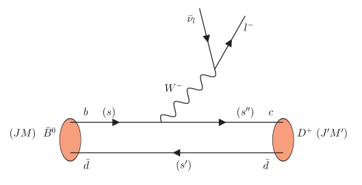
Figure 1: Diagrammatic representation of $\bar{B}^{0}\to\bar{\nu}_{l}l^{-}D^{+}$ at the quark level.

The weak interaction is given by the Hamiltonian

$$H=\mathcal{C}L^{\alpha}Q_{\alpha}\,,$$ (1)

where in $\mathcal{C}$ one has the couplings of the weak interaction, but, since we are only concerned about ratios of rates, it plays no role in our study. The leptonic current is given by

$$L^{\alpha}=\langle{\bar{u}}_{l}|\gamma^{\alpha}(1-\gamma_{5})|v_{\nu}\rangle\,,$$ (2)

and $Q^{\alpha}$, the quark current, by

$$Q^{\alpha}=\langle{\bar{u}}_{c}|\gamma^{\alpha}(1-\gamma_{5})|u_{b}\rangle\,.$$ (3)

In order to obtain the $\bar{B}^{0}$ decay width we need

$$\sum_{\rm lep~{}pol}L^{\alpha}{L^{\beta}}^{*}~{}\overline{\sum_{quark}}\sum_{\rm pol}Q_{\alpha}Q_{\beta}^{*}\equiv{L}^{\alpha\beta}\overline{\sum}\sum Q_{\alpha}Q_{\beta}^{*}\,,$$ (4)

where ${L}^{\alpha\beta}$ stands for ${\sum_{\rm pol}}L^{\alpha}{L^{\beta}}^{*}$ and is easily evaluated with the result Navarra

$${L}^{\alpha\beta}=2~{}\frac{p_{\nu}^{\alpha}p_{l}^{\beta}+p_{l}^{\alpha}p_{\nu}^{\beta}-p_{\nu}\cdot p_{l}g^{\alpha\beta}-i\epsilon^{\rho\alpha\sigma\beta}p_{\nu\rho}p_{l\sigma}}{m_{\nu}m_{l}}\,,$$ (5)

where we adopt the Mandl and Shaw normalization for fermions mandl . The mass of the neutrino and the lepton get cancelled in the final formula of the width.

In Ref. Navarra a similar sum and an average and sum over the quark spin third components was done. Here we pay a special attention to the vector or pseudoscalar components, and the coupling of spins to given quantum numbers has to be done prior to the sums over the third components in the final $Q_{\alpha}Q_{\beta}^{*}$ term. For this purpose we must evaluate explicitly the quark current $Q_{\alpha}$. We use the ordinary spinors Itzykson

$$u_{r}=\widetilde{A}\left(\begin{array}[]{c}\chi_{r}\\ \widetilde{B}{\bm{\sigma}}\cdot{\bm{p}}\,\chi_{r}\end{array}\right)\,;\qquad\widetilde{A}=\left(\frac{E_{p}+m}{2\,m}\right)^{1/2}\,;\qquad\widetilde{B}=\frac{1}{E_{p}+m}\,,$$ (6)

where $\chi_{r}$ are the Pauli bispinors and $m,p$ and $E_{p}$ are the mass, momentum and energy of the quark. Next we use Navarra

$$\frac{p_{b}}{m_{b}}=\frac{p_{B}}{m_{B}}\,;\qquad\frac{E_{b}}{m_{b}}=\frac{E_{B}}{m_{B}}\,,$$ (7)

and the same for the $c$ quark. Theses ratios are related to the velocity of the quarks or $B$ mesons and neglect the internal motion of the quarks inside the meson. We evaluate the matrix elements in the frame where the ${\bar{\nu}}l$ system is at rest, where ${\bm{p}}_{B}={\bm{p}}_{D}={\bm{p}}$ and both have a sizeable velocity. We have in general

$$p=\frac{\lambda^{1/2}(m_{in}^{2},M_{\rm inv}^{2(\nu l)},m^{2}_{fin})}{2M_{\rm inv}^{(\nu l)}}\,,$$ (8)

where $m_{in}$, $m_{fin}$ are the masses of the initial, final mesons in the decay, and $M_{\rm inv}^{(\nu l)}$ is the invariant mass of the $\nu l$ pair. Using Eq. (7) we can now write

$$u_{r}=A\left(\begin{array}[]{c}\chi_{r}\\ B{\bm{\sigma}}\cdot{\bm{p}}_{B}\,\chi_{r}\end{array}\right)\,;\qquad A=\left(\frac{\frac{E_{B}}{m_{B}}+1}{2}\right)^{1/2}\,;\qquad B=\frac{1}{m_{B}(1+\frac{E_{B}}{m_{B}})}\,.$$ (9)

We also use the $\gamma^{\mu}$ representation of Ref. Itzykson

$$\gamma^{0}=\left(\begin{array}[]{cc}~{}I{}&~{}0{}\\ 0&-I\end{array}\right);\qquad\gamma_{5}=\left(\begin{array}[]{cc}~{}0{}&~{}I{}\\ ~{}I{}&~{}0{}\end{array}\right);\qquad\gamma^{i}=\left(\begin{array}[]{cc}~{}0{}&\sigma^{i}\\ -\sigma^{i}&~{}0{}\end{array}\right)\,,~{}~{}i=1,2,3\,.$$ (10)

As a consequence we have

$$\gamma^{0}-\gamma^{0}\gamma_{5}=\left(\begin{array}[]{cc}~{}I{}&~{}-I{}\\ I&-I\end{array}\right);\qquad\gamma^{i}-\gamma^{i}\gamma_{5}=\left(\begin{array}[]{cc}~{}-\sigma^{i}{}&~{}\sigma^{i}{}\\ -\sigma^{i}&\sigma^{i}\end{array}\right)\,.$$ (15)

where we denote the Pauli matrices as $\sigma^{i}$, $\sigma_{i}$ (i=1,2,3), but they are the same thing.

$$\langle{\bar{u}}_{c}|\gamma^{0}-\gamma^{0}\gamma_{5}|u_{b}\rangle=AA^{\prime}\left\{(1+BB^{\prime}p^{2})\langle\chi_{c}|\chi_{b}\rangle-(B+B^{\prime})\langle\chi_{c}|{\bm{\sigma}}\cdot{\bm{p}}|\chi_{b}\rangle\right\}\,,$$ (16)

where $p^{2}$ stands for ${\bm{p}}^{2}$ from here on, and $A^{\prime},B^{\prime}$ stand for the $D$ meson.

Similarly,

$$\langle{\bar{u}}_{c}|\gamma^{i}-\gamma^{i}\gamma_{5}|u_{b}\rangle = AA^{\prime}\left\{-\langle\chi_{c}|{{\sigma}}^{i}|\chi_{b}\rangle+B\langle\chi_{c}|{{\sigma}}^{i}\,{\bm{\sigma}}\cdot{\bm{p}}|\chi_{b}\rangle\right.$$ (17)

$$+ \left.B^{\prime}\langle\chi_{c}|{\bm{\sigma}}\cdot{\bm{p}}\,{{\sigma}}^{i}|\chi_{b}\rangle-BB^{\prime}\langle\chi_{c}|{\bm{\sigma}}\cdot{\bm{p}}\,{{\sigma}}^{i}\,{\bm{\sigma}}\cdot{\bm{p}}|\chi_{b}\rangle\right\}\,.$$

The explicit calculation is simplified if we take ${\bm{p}}$ in the $z$ direction. Then, considering the spins, $s$,$s^{\prime\prime}$, $s^{\prime}$ (of the $\bar{d}$ in the ${\bm{p}}$ direction) of Fig. 1 one has

$$\langle\chi_{c}|{\bm{\sigma}}\cdot{\bm{p}}|\chi_{b}\rangle=p\,\langle s^{\prime\prime}|\sigma_{z}|s\rangle=p\,(-1)^{\frac{1}{2}-s}\delta_{ss^{\prime\prime}}\equiv p\,\sqrt{3}\,{\cal C}(\frac{1}{2}1\frac{1}{2};s,0,s^{\prime\prime})\delta_{ss^{\prime\prime}}\,,$$ (18)

where in the last step we evaluate the $\sigma_{z}$ matrix element using the Wigner-Eckart Theorem. Hence,

$$\langle{\bar{u}}_{c}|\gamma^{0}-\gamma^{0}\gamma_{5}|u_{b}\rangle\equiv M_{0} = AA^{\prime}\left\{(1+BB^{\prime}p^{2})\delta_{ss^{\prime\prime}}-(B+B^{\prime})\,p\,\delta_{ss^{\prime\prime}}\,\sqrt{3}\,{\cal C}(\frac{1}{2}1\frac{1}{2};s,0,s^{\prime\prime})\right\}~{}~{}~{}~{}$$ (19)

$$= AA^{\prime}\delta_{ss^{\prime\prime}}\left\{1+BB^{\prime}p^{2}-(B+B^{\prime})\,p\,\sqrt{3}\,{\cal C}(\frac{1}{2}1\frac{1}{2};s,0,s)\right\}\,.$$

$$\langle{\bar{u}}_{c}|\gamma^{i}-\gamma^{i}\gamma_{5}|u_{b}\rangle\equiv N_{i} = AA^{\prime}\left\{-\langle s^{\prime\prime}|{{\sigma}}^{i}|s\rangle+B\,p\,\langle s^{\prime\prime}|{{\sigma}}^{i}\sigma_{z}|s\rangle+B^{\prime}\,p\,\langle s^{\prime\prime}|\sigma_{z}{{\sigma}}^{i}|s\rangle-BB^{\prime}\,p^{2}\,\langle s^{\prime\prime}|\sigma_{z}{{\sigma}}^{i}\sigma_{z}|s\rangle\right\}~{}~{}~{}~{}~{}$$ (20)

$$= AA^{\prime}\left\{-\langle s^{\prime\prime}|{{\sigma}}^{i}|s\rangle+B\,p\,\langle s^{\prime\prime}|{{\sigma}}^{i}|s\rangle(-1)^{\frac{1}{2}-s}+B^{\prime}\,p\,\langle s^{\prime\prime}|{{\sigma}}^{i}|s\rangle(-1)^{\frac{1}{2}-s^{\prime\prime}}\right.$$

$$\left.-BB^{\prime}p^{2}(-1)^{\frac{1}{2}-s}(-1)^{\frac{1}{2}-s^{\prime\prime}}\langle s^{\prime\prime}|{{\sigma}}^{i}|s\rangle\right\}\,.$$

If we keep the covariant form $\gamma_{i}-\gamma_{i}\gamma_{5}$ we have

$$\langle{\bar{u}}_{c}|\gamma_{i}-\gamma_{i}\gamma_{5}|u_{b}\rangle=AA^{\prime}\langle s^{\prime\prime}|{{\sigma}}^{i}|s\rangle\left\{1-B\,p\,(-1)^{\frac{1}{2}-s}-B^{\prime}\,p\,(-1)^{\frac{1}{2}-s^{\prime\prime}}+BB^{\prime}p^{2}(-1)^{1-s-s^{\prime\prime}}\right\}~{}~{}~{}~{}~{}\,.$$ (21)

In order to work out the angular momentum algebra it is more convenient to evaluate the spherical component of ${{\sigma}}^{i}\to{{\sigma}}_{\mu},\mu=1,0,-1$ in the last equation, and we define, $M_{0}$ for the $\gamma^{0}-\gamma^{0}\gamma_{5}$ matrix element of Eq. (19) and $N_{\mu}$ for the matrix element of Eq. (20) substituting ${{\sigma}}^{i}$ by ${{\sigma}}_{\mu}$.

The explicit evaluation is done in the Appendix for the $M_{0}$ and $N_{\mu}$ matrix elements and we show here the results.

• $M_{0}$ matrix element

  • $J=0,J^{\prime}=0$

    $$M_{0}=AA^{\prime}(1+BB^{\prime}\,p^{2}\,)\delta_{M0}\,\delta_{M^{\prime}0}$$ (22)

  • $J=0,J^{\prime}=1$

    $$M_{0}=-AA^{\prime}(B+B^{\prime})p\delta_{M0}\,\delta_{M^{\prime}0}$$ (23)

  • $J=1,J^{\prime}=0$

    $$M_{0}=-AA^{\prime}(B+B^{\prime})p\delta_{M0}\,\delta_{M^{\prime}0}$$ (24)

  • $J=1,J^{\prime}=1$

    $$M_{0}=AA^{\prime}\left\{(1+BB^{\prime}p^{2})-\sqrt{2}(B+B^{\prime})\,p\,{\cal C}(111;M,0,M)\right\}\delta_{MM^{\prime}}$$ (25)

• $N_{\mu}$ matrix element

  • $J=0,J^{\prime}=0$

    $$N_{\mu}=-AA^{\prime}(B+B^{\prime})p\delta_{M0}\,\delta_{M^{\prime}0}\,\delta_{\mu 0}$$ (26)

  • $J=0,J^{\prime}=1$

    $$N_{\mu}=AA^{\prime}\left\{1+BB^{\prime}p^{2}\,(-1)^{-M^{\prime}}+\sqrt{2}(Bp+B^{\prime}p(-1)^{-M^{\prime}}){\cal C}(111;M^{\prime},0,M^{\prime})\right\}\delta_{\mu,M^{\prime}}\,\delta_{M0}$$ (27)

  • $J=1,J^{\prime}=0$

    $$N_{\mu} = AA^{\prime}\left\{(1+BB^{\prime}\,p^{2}\,(-1)^{M})(-1)^{-M}~{}~{}~{}~{}\right.$$ (28)

    $$- \left.\sqrt{2}(-1)^{M}(Bp+B^{\prime}p(-1)^{M})\,{\cal C}(111;M,0,M)\right\}\delta_{\mu M}\,\delta_{M^{\prime}0}$$

  • $J=1,J^{\prime}=1$

    $$N_{\mu} = AA^{\prime}\left\{(1+BB^{\prime}p^{2}(-1)^{M-M^{\prime}})\sqrt{2}\,{\cal C}(111;M,M^{\prime}-M,M^{\prime})-(Bp+B^{\prime}p(-1)^{M-M^{\prime}})\delta_{M0}~{}~{}~{}~{}~{}\right.$$ (29)

    $$- \left.2(Bp+B^{\prime}p(-1)^{M-M^{\prime}})\,{\cal C}(111;M^{\prime}-M,M,M^{\prime})\,{\cal C}(111;0,M,M)\right\}\delta_{\mu,M^{\prime}-M}$$

• Next we must evaluate ${L}^{\alpha\beta}Q_{\alpha}Q_{\beta}^{*}$ and sum and average over polarizations. In terms of the $M_{0}$ and $N_{i}$ terms defined before we have the combination

  $$\overline{\sum}\sum\left|t\right|^{2}=L^{00}M_{0}~{}M^{*}_{0}+L^{0i}M_{0}~{}N^{*}_{i}+L^{i0}N_{i}~{}M_{0}^{*}+L^{ij}N_{i}~{}N_{j}^{*}\,.$$ (30)

  The explicit evaluation is done in the Appendix and we show here the final results.

  • $J=0,J^{\prime}=0$

    $$\overline{\sum}\sum|t|^{2} = \frac{(AA^{\prime})^{2}}{m_{\nu}m_{l}}\left\{\frac{m^{2}_{l}(M_{\rm inv}^{2(\nu l)}-m^{2}_{l})}{M_{\rm inv}^{2(\nu l)}}\left(1+BB^{\prime}\,p^{2}\right)^{2}\right.$$ (31)

    $$+ \left.2\,\left(\widetilde{E}_{\nu}\widetilde{E}_{l}+\frac{1}{3}\widetilde{p}_{\nu}^{2}\right)(B+B^{\prime})^{2}p^{2}\right\}\,,$$

    where the magnitudes with tilda are evaluated in the $\nu l$ rest frame. Thus

    $$\widetilde{E}_{l}=\frac{M_{\rm inv}^{2(\nu l)}+m^{2}_{l}-m^{2}_{\nu}}{2\,M_{\rm inv}^{(\nu l)}}\,,$$

    $$\widetilde{E}_{\nu}=\frac{M_{\rm inv}^{2(\nu l)}+m^{2}_{\nu}-m^{2}_{l}}{2\,M_{\rm inv}^{(\nu l)}}\,,$$

    $$\widetilde{p}_{\nu}=\frac{\lambda^{1/2}(M_{\rm inv}^{2(\nu l)},m^{2}_{\nu},m^{2}_{l})}{2M_{\rm inv}^{(\nu l)}}\,.$$ (32)

  • $J=0,J^{\prime}=1$

    $$\overline{\sum}\sum|t|^{2} = \frac{(AA^{\prime})^{2}}{m_{\nu}m_{l}}\left\{\frac{m^{2}_{l}(M_{\rm inv}^{2(\nu l)}-m^{2}_{l})}{M_{\rm inv}^{2(\nu l)}}(B+B^{\prime})^{2}p^{2}\right.$$ (33)

    $$+ \left.2\,\left(\widetilde{E}_{\nu}\widetilde{E}_{l}+\frac{1}{3}\widetilde{p}^{2}_{\nu}\right)\left(3-6BB^{\prime}p^{2}+2(B^{2}+B^{\prime 2})p^{2}+3(BB^{\prime}p^{2})^{2}\right)\right\}\,,$$

  • $J=1,J^{\prime}=0$

    $$\overline{\sum}\sum|t|^{2}=\frac{1}{3}\,\overline{\sum}\sum|t|^{2}(J=0,J^{\prime}=1)\,,$$ (34)

    where the factor $\frac{1}{3}$ comes because we average over the initial $J=1$ polarizations.

  • $J=1,J^{\prime}=1$

    $$\overline{\sum}\sum|t|^{2} = \frac{1}{3}\,\frac{(AA^{\prime})^{2}}{m_{\nu}m_{l}}\left\{\frac{3\,m^{2}_{l}(M_{\rm inv}^{2(\nu l)}-m^{2}_{l})}{M_{\rm inv}^{2(\nu l)}}\left[(1+BB^{\prime}p^{2})^{2}+\frac{2}{3}(B+B^{\prime})^{2}p^{2}\right]\right.$$ (35)

    $$+ \left.2\,\left(\widetilde{E}_{\nu}\widetilde{E}_{l}+\frac{1}{3}\widetilde{p}^{2}_{\nu}\right)\left[6+7(B^{2}+B^{\prime 2})p^{2}-4BB^{\prime}p^{2}+6(BB^{\prime}p^{2})^{2}\right]\right\}.~{}~{}~{}~{}~{}~{}\,$$

These techniques have also been used successfully in the evaluation of weak decays $M_{1}\to M_{2}M_{3}$ liangoset and in $\tau^{-}\to M_{1}M_{2}$ decays daioset .

III Results

The invariant mass distribution $d\Gamma/dM_{\rm inv}^{(\nu l)}$ is given for $B\to\bar{\nu}lD$ by

$$\frac{d\Gamma}{dM_{\rm inv}^{(\nu l)}}=\frac{2m_{\nu}2m_{l}}{(2\pi)^{3}}\,\frac{1}{4M^{2}_{B}}p_{D}\widetilde{p}_{\nu}\overline{\sum}\sum|t|^{2}\,,$$ (36)

where $p_{D}$ is the $D$ momentum in the $B$ rest frame and $\widetilde{p}_{\nu}$ the $\bar{\nu}$ momentum in the $\nu l$ rest frame,

$$p_{D}=\frac{\lambda^{1/2}(m^{2}_{B},M_{\rm inv}^{2(\nu l)},m^{2}_{D})}{2m_{B}}\,.$$ (37)

By integrating $d\Gamma/dM_{\rm inv}^{(\nu l)}$ over $M_{\rm inv}^{(\nu l)}$ we obtain the width that we show in the tables.

III.1 $B$ and $B^{*}$ decays

We study only the most Cabibbo-favored processes, $b\to c$ and $c\to s$. We show in Table 1 the $\bar{B}$, $\bar{B}_{s}$ and $\bar{B}_{c}$ semileptonic decays. Since we can only provide ratios, we fix one decay rate to the experiment and the rest are predictions, In this case we fix our rate to ${B}^{-}\to D^{0}~{}e^{-}~{}\bar{\nu}_{e}$ . We then observe that the predictions done for six decays are all in agreement with experiment, except for the $\bar{B}^{0}\to D^{+}~{}\tau^{-}\bar{\nu}_{\tau}$ that we will discuss later. The $e^{-}~{}\bar{\nu}_{e}$ and $\mu^{-}\bar{\nu}_{\mu}$ decay rates are very similar, since the masses of $e^{-}$ and $\mu^{-}$ are very small compared to the meson masses. The term proportional to $m^{2}_{l}$ in Eq. (68) is negligible for $e^{-}$ and $\mu^{-}$, but not for $\tau^{-}$. This term is responsible for a bigger rate than expected from phase space for the $\tau^{-}\bar{\nu}_{\tau}$ decays. In Table 1 we also show predictions for $\bar{B}^{0}_{s}$ and $B^{-}_{c}$ decays, for which there are not yet experimental data in the PDG pdg . For the $\bar{B}^{0}\to D^{+}~{}\tau^{-}\bar{\nu}_{\tau}$ we get a rate about a factor of two smaller than experiment. This has to be seen from the perspective that we are implicitly using the same form factors as for $\bar{B}^{0}\to D^{+}~{}e^{-}~{}\bar{\nu}_{e}$. However, because of the larger $\tau^{-}$ mass, the momentum transfers are smaller in this latter case and by taking the same form factors as in $\bar{B}^{0}\to D^{+}~{}e^{-}~{}\bar{\nu}_{e}$ we are reducing the $\bar{B}^{0}\to D^{+}~{}\tau^{-}\bar{\nu}_{\tau}$ rate more than one should. This is telling us implicitly the strength of the form factors in the present reactions. For ${B}^{-}\to D^{0}~{}\tau^{-}\bar{\nu}_{\tau}$ the experimental error is relatively large, such that the rate is compatible with the theoretical one, but also with double its value.

We would like to call the attention to the rates for ${B}^{-}\to D^{0}~{}e^{-}~{}\bar{\nu}_{e}$ (${B}^{-}\to D^{0}~{}\mu^{-}\bar{\nu}_{\mu}$). These rates are identical experimentally within experimental errors, and also theoretically (up to small difference due to the different masses of the mesons). This should be the case, since from one reaction to the other the only change has been to substitute the $\bar{d}$ spectator quark in Fig. 1 by a $\bar{u}$.

Table 1: Branching ratios for ${\color[rgb]{0,0,1}(PP)}$ semileptonic decay of $B$ meson. We consider the same mean life $\tau$ for $\bar{B}^{0}$,${B}^{-}$, $\bar{B}^{0}_{s}$, but $\frac{\tau(B^{-}_{c})}{\tau(B^{-})}=0.31$

Decay process	BR (Theo.)	BR (Exp.)pdg
$\bar{B}^{0}\to D^{+}~{}e^{-}~{}\bar{\nu}_{e}$	$2.19\times 10^{-2}$	$(2.19\pm 0.12)\times 10^{-2}$
$\bar{B}^{0}\to D^{+}~{}\mu^{-}\bar{\nu}_{\mu}$	$2.17\times 10^{-2}$	$(2.19\pm 0.12)\times 10^{-2}$
$\bar{B}^{0}\to D^{+}~{}\tau^{-}\bar{\nu}_{\tau}$	$4.97\times 10^{-3}$	$(1.03\pm 0.22)\times 10^{-2}$
${B}^{-}\to D^{0}~{}e^{-}~{}\bar{\nu}_{e}$	fit the exp	$(2.20\pm 0.11)\times 10^{-2}$
${B}^{-}\to D^{0}~{}\mu^{-}\bar{\nu}_{\mu}$	$2.19\times 10^{-2}$	$(2.20\pm 0.11)\times 10^{-2}$
${B}^{-}\to D^{0}~{}\tau^{-}\bar{\nu}_{\tau}$	$5.02\times 10^{-3}$	$(7.7\pm 2.5)\times 10^{-3}$
$\bar{B}^{0}_{s}\to D^{+}_{s}~{}e^{-}~{}\bar{\nu}_{e}$	$2.07\times 10^{-2}$
$\bar{B}^{0}_{s}\to D^{+}_{s}~{}\mu^{-}\bar{\nu}_{\mu}$	$2.07\times 10^{-2}$
$\bar{B}^{0}_{s}\to D^{+}_{s}~{}\tau^{-}\bar{\nu}_{\tau}$	$4.69\times 10^{-3}$
$B^{-}_{c}\to\eta_{c}~{}e^{-}~{}\bar{\nu}_{e}$	$3.93\times 10^{-3}$
$B^{-}_{c}\to\eta_{c}~{}\mu^{-}\bar{\nu}_{\mu}$	$3.90\times 10^{-3}$
$B^{-}_{c}\to\eta_{c}~{}\tau^{-}\bar{\nu}_{\tau}$	$8.49\times 10^{-4}$

Table 2: The same as Table 1 but for ${\color[rgb]{0,0,1}(PV)}$ case.

Decay process	BR (Theo.)	BR (Exp.)pdg
$\bar{B}^{0}\to D^{*+}~{}e^{-}~{}\bar{\nu}_{e}$	$4.86\times 10^{-2}$	$(4.93\pm 0.11)\times 10^{-2}$
$\bar{B}^{0}\to D^{*+}~{}\mu^{-}\bar{\nu}_{\mu}$	$4.83\times 10^{-2}$	$(4.93\pm 0.11)\times 10^{-2}$
$\bar{B}^{0}\to D^{*+}~{}\tau^{-}\bar{\nu}_{\tau}$	$1.03\times 10^{-2}$	$(1.67\pm 0.13)\times 10^{-2}$
${B}^{-}\to D^{*0}~{}e^{-}~{}\bar{\nu}_{e}$	$4.88\times 10^{-2}$	$(5.69\pm 0.19)\times 10^{-2}$
${B}^{-}\to D^{*0}~{}\mu^{-}\bar{\nu}_{\mu}$	$4.86\times 10^{-2}$	$(5.69\pm 0.19)\times 10^{-2}$
${B}^{-}\to D^{*0}~{}\tau^{-}\bar{\nu}_{\tau}$	$1.04\times 10^{-2}$	$(1.88\pm 0.2)\times 10^{-2}$
$\bar{B}^{0}_{s}\to D^{*+}_{s}~{}e^{-}~{}\bar{\nu}_{e}$	$4.60\times 10^{-2}$
$\bar{B}^{0}_{s}\to D^{*+}_{s}~{}\mu^{-}\bar{\nu}_{\mu}$	$4.58\times 10^{-2}$
$\bar{B}^{0}_{s}\to D^{*+}_{s}~{}\tau^{-}\bar{\nu}_{\tau}$	$9.64\times 10^{-3}$
$B^{-}_{c}\to J/\psi~{}e^{-}~{}\bar{\nu}_{e}$	$9.47\times 10^{-3}$
$B^{-}_{c}\to J/\psi~{}\mu^{-}\bar{\nu}_{\mu}$	$9.41\times 10^{-3}$
$B^{-}_{c}\to J/\psi~{}\tau^{-}\bar{\nu}_{\tau}$	$1.88\times 10^{-3}$

In Table 2 we show results for $\bar{B}$ decays into $D^{*}$ and related reactions. This corresponds to the case $J=0,J^{\prime}=1$ studied in the former sections. We do not fit now one rate, because the idea is to make a prediction for these decays based on the $B\to D$ reactions. We can see that the predicted rates for the case of light leptons are compatible with experiment, This should be seen as an accomplishment of the present framework, which shows that assuming the same form factors for $D$ or $D^{*}$ decay, as we would induce from heavy quark symmetry nieves , the rates for these two decays are a consequence of the angular momentum structure with the dynamics of the weak interaction.

We can also observe that the branching ratio for $\bar{B}^{0}\to D^{*+}~{}\tau^{-}\bar{\nu}_{\tau}$ is about a factor $0.61$ the experimental one, in line with what was observed in Table 1. The same happens for ${B}^{-}\to D^{*0}~{}\tau^{-}\bar{\nu}_{\tau}$ where the reduction factor is about $0.55$. Yet, if we evaluate the ratio of the rates of $\bar{B}^{0}\to D^{*+}~{}\tau^{-}\bar{\nu}_{\tau}$ to $\bar{B}^{0}\to D^{+}~{}\tau^{-}\bar{\nu}_{\tau}$ we find a factor of $2.07$ against $1.62\pm 0.37$ experimentally, or $2.07$ for the ratio of rates of ${B}^{-}\to D^{*0}~{}\tau^{-}\bar{\nu}_{\tau}$ to $\bar{B}^{-}\to D^{0}~{}\tau^{-}\bar{\nu}_{\tau}$ versus $2.44\pm 0.83$ experimentally. One expects these two ratios to be the same, and so they are experimentally within errors, and also compatible with the theory.

Once again we make predictions for six more decay modes. It is interesting to observe that the rates for ${B}^{-}\to\bar{D}^{*}\bar{\nu}_{l}$ are bigger experimentally than those of ${B}^{-}\to\bar{D}\bar{\nu}_{l}$, something that is also obtained theoretically.

Recently much work has been devoted to the ratios

$$R_{D} = \frac{BR({B}^{-}\to D\bar{\nu}_{\tau}\tau)}{BR({B}^{-}\to D\bar{\nu}_{l}l)}=0.407\pm 0.039\pm 0.024\,,$$

$$R_{D^{*}} = \frac{BR({B}^{-}\to D^{*}\bar{\nu}_{\tau}\tau)}{BR({B}^{-}\to D^{*}\bar{\nu}_{l}l)}=0.304\pm 0.013\pm 0.007\,,$$ (38)

from where one expects to observe new physics Fajfer ; German . The values in Eq. (III.1) are taken from the HFLAV collaboration average HFLAV . The most precise single measurement performed so far is the recent one of the LHCb Collaboration lhcbd $R_{D^{*}}=0.291\pm 0.019\pm 0.026\pm 0.013$. Our result for these ratios are $R_{D}=0.23$, $R_{D^{*}}=0.211$. As we can see, both $R_{D}$ and $R_{D^{*}}$ are smaller than experiment for the reasons discussed above. To put our results in perspective we can compare these result with Lattice results lat1 ; lat2 which give $R_{D}=0.299\pm 0.011$, and calculations based on the standard model obtaining ratios of form factors from experiment Fajfer which give $R_{D^{*}}=0.252\pm 0.03$. This latter case is increased to $0.27$ in Genaro by taking into account in the theoretical evaluation that $D^{*}\to D\pi$, the mode where the $D^{*}$ is observed experimentally.

Another ratio of interest is

$$R_{J/\psi}=\frac{BR(B^{+}_{c}\to J/\psi~{}{\nu}_{\tau}\tau^{+})}{BR(B^{+}_{c}\to J/\psi~{}{\nu}_{\mu}\mu^{+})}=0.71\pm 0.12\pm 0.18\,,$$ (39)

reported by LHCb lhcbj . We obtain $0.20$ for this ratio, short of the experimental one even considering errors, and one must find the reason in the discussion in former points since momentum transfer for $B^{+}_{c}\to J/\psi~{}\tau^{+}{\nu}_{\tau}$ is smaller than in $B^{+}_{c}\to J/\psi~{}\mu^{+}{\nu}_{\mu}$. It is also useful to compare our results with other theoretical works based on the standard model which provide value around $0.25\sim 0.28$ Semay ; Kiselev ; Ivanov ; eli for this ratio.

There is another remark we can do in view of our easy expressions for $\overline{\sum}\sum|t|^{2}$. If one looks at Eq. (68) for $J=0,J^{\prime}=0$, one can see that the term independent of $p$ is proportional to $m^{2}_{l}$, which is very small for light leptons. The important term is this case is the second term of that equation, proportional to $p^{2}$. This tells us that nonrelativistic calculations, which would neglect this momentum, or the strict use of heavy quark symmetry, neglecting terms of $O(\frac{p}{m_{Q}})$ (see $B$ factor in Eq. (9)), would provide very bad results for the rate of $\bar{B}\to D$ and light leptons.

Table 3: Widths for ${\color[rgb]{0,0,1}(VP)}$ semileptonic decay of $B^{*}$ mesons in units of $\Gamma(B^{-}\to{D}^{0}e^{-}~{}\bar{\nu}_{e})$.

Decay process	$\Gamma$ (Theo.)	$\Gamma$ (Ref. wangwang )	$\Gamma$ (Ref. changyang )
$\bar{B}^{*0}\to D^{+}~{}e^{-}~{}\bar{\nu}_{e}$	0.95
$\bar{B}^{*0}\to D^{+}~{}\mu^{-}\bar{\nu}_{\mu}$	0.95
$\bar{B}^{*0}\to D^{+}~{}\tau^{-}\bar{\nu}_{\tau}$	0.24
${B}^{*-}\to D^{0}~{}e^{-}~{}\bar{\nu}_{e}$	0.96	1.74	1.21
${B}^{*-}\to D^{0}~{}\mu^{-}\bar{\nu}_{\mu}$	0.96	1.73	1.21
${B}^{*-}\to D^{0}~{}\tau^{-}\bar{\nu}_{\tau}$	0.24	0.43	0.36
$\bar{B}^{*0}_{s}\to D^{+}_{s}~{}e^{-}~{}\bar{\nu}_{e}$	0.91	1.57	1.07
$\bar{B}^{*0}_{s}\to D^{+}_{s}~{}\mu^{-}\bar{\nu}_{\mu}$	0.91	1.56	1.07
$\bar{B}^{*0}_{s}\to D^{+}_{s}~{}\tau^{-}\bar{\nu}_{\tau}$	0.23	0.41	0.31
${B^{*-}_{c}}\to\eta_{c}~{}e^{-}~{}\bar{\nu}_{e}$	0.59	1.09
${B^{*-}_{c}}\to\eta_{c}~{}\mu^{-}\bar{\nu}_{\mu}$	0.58	1.09
${B^{*-}_{c}}\to\eta_{c}~{}\tau^{-}\bar{\nu}_{\tau}$	0.14	0.33

In Table 3 we also show the rate for the semileptonic decays of $\bar{B}^{*}\to D$. These decay rates have not been observed and one reason maybe the fact that $B^{*}$ decays electromagnetically in $\gamma B$. In Ref. wangwang these rates were evaluated using the Bethe-Salpeter approach with the instantaneous approximation. We compare our predictions with those in Ref. wangwang . These decay widths are also evaluated in Ref. changyang in the Baner-Stech-Wirbel model and in Table 3 we also show these results. Our results are qualitatively similar to those of changyang , about $25\%$ smaller and also smaller than those of wangwang by a factor of about $0.6$. One should stress the simplicity of our approach with respect to wangwang where 14 form factors are evaluated and the theory relies on several parameters zhangwang , partly constrained from the masses of the mesons. We should stress that the rates for $B^{*}\to D\bar{\nu}l$ in our approach involve the same matrix element as for $B\to D^{*}\bar{\nu}l$ ($J=1,J^{\prime}=0$, versus $J=0,J^{\prime}=1$ in Eqs. (33),(34)). Given the accuracy by which we predicted the rate for $B\to D^{*}\bar{\nu}l$ in Table 2, our predicted rates for $B^{*}\to D\bar{\nu}l$ should be equally accurate. Yet, seen from the perspective that these are the first theoretical predictions for $B^{*}$ decay rates, the main message is that the three calculations reported provide very similar numbers and this should be sufficient for planning possible experimental searches.

We complete this part by making predictions for $B^{*}\to D^{*}\nu l$ in Table 4, in which we also compare our results with those obtained in Ref. wangwang . We observe now that in both cases the widths are much bigger than for $B^{*}\to D\nu l$, and our predictions are again a factor of about $0.55$ those of Ref. wangwang , with a bit bigger discrepancies for decays in the $\tau$ mode, as we would expect.

Table 4: The same as Table 3 but for ${\color[rgb]{0,0,1}(VV)}$ case.

Decay process	$\Gamma$ (Theo.)	$\Gamma$ (Ref. wangwang )
$\bar{B}^{*0}\to D^{*+}~{}e^{-}~{}\bar{\nu}_{e}$	2.52
$\bar{B}^{*0}\to D^{*+}~{}\mu^{-}\bar{\nu}_{\mu}$	2.50
$\bar{B}^{*0}\to D^{*+}~{}\tau^{-}\bar{\nu}_{\tau}$	0.51
${B}^{*-}\to D^{*0}~{}e^{-}~{}\bar{\nu}_{e}$	2.53	4.98
${B}^{*-}\to D^{*0}~{}\mu^{-}\bar{\nu}_{\mu}$	2.51	4.95
${B}^{*-}\to D^{*0}~{}\tau^{-}\bar{\nu}_{\tau}$	0.51	1.08
$\bar{B}^{*0}_{s}\to D^{*+}_{s}~{}e^{-}~{}\bar{\nu}_{e}$	2.40	4.40
$\bar{B}^{*0}_{s}\to D^{*+}_{s}~{}\mu^{-}\bar{\nu}_{\mu}$	2.37	4.38
$\bar{B}^{*0}_{s}\to D^{*+}_{s}~{}\tau^{-}\bar{\nu}_{\tau}$	0.48	1.00
${B^{*-}_{c}}\to J/\psi~{}e^{-}~{}\bar{\nu}_{e}$	1.60	2.95
${B^{*-}_{c}}\to J/\psi~{}\mu^{-}\bar{\nu}_{\mu}$	1.58	2.94
${B^{*-}_{c}}\to J/\psi~{}\tau^{-}\bar{\nu}_{\tau}$	0.31	0.82

Figure 2: The differential width of semileptonic decay of $B$ meson decay.

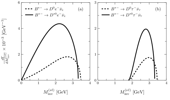
Figure 3: The differential width of semileptonic decay of $B^{*}$ meson decay.

It is also interesting to look into the invariant mass distribution $d\Gamma/dM_{\rm inv}^{(\nu l)}$. In Fig. 2 we show $d\Gamma/dM_{\rm inv}^{(\nu l)}$ for ${B}^{-}\to D^{0}~{}e^{-}~{}\bar{\nu}_{e}$, ${B}^{-}\to D^{*0}~{}e^{-}~{}\bar{\nu}_{e}$, and ${B}^{-}\to D^{0}~{}\tau^{-}\bar{\nu}_{\tau}$, ${B}^{-}\to D^{*0}~{}\tau^{-}\bar{\nu}_{\tau}$. In the case of ${B}^{-}\to D^{0}~{}e^{-}~{}\bar{\nu}_{e}$ the mass distribution peaks around $1.7~{}\rm{GeV}$ while for ${B}^{-}\to D^{*0}~{}e^{-}~{}\bar{\nu}_{e}$ it peaks around $2.7~{}\rm{GeV}$. This difference is surprising in view of the small difference of mass between $D$ and $D^{*}$. One must see the reason for this behaviour in the structure of Eqs. (68) and (33). As we mentioned before, the ${B}^{-}\to D^{0}~{}e^{-}~{}\bar{\nu}_{e}$ reaction gets most of its strength from the $p^{2}$ term of Eq. (68) since the $m^{2}_{l}$ term is extremely small. One gets a bigger contribution the larger $p^{2}$, but this means a smaller $M_{\rm inv}^{(\nu l)}$(see Eq. (8)). In the case of ${B}^{-}\to D^{*0}~{}e^{-}~{}\bar{\nu}_{e}$, Eq.(33) there are large terms independent of $p$ and the argument does not hold. In the case of ${B}^{-}\to D^{0}~{}\tau^{-}\bar{\nu}_{\tau}$ and ${B}^{-}\to D^{*0}~{}\tau^{-}\bar{\nu}_{\tau}$, the $m^{2}_{l}$ term is not so small and the position of the peaks is much closer. The argument discussed above become even more clear when we look at the distributions of Fig. 3 for ${B}^{*-}\to D^{0}~{}e^{-}~{}\bar{\nu}_{e}$, ${B}^{*-}\to D^{*0}~{}e^{-}~{}\bar{\nu}_{e}$ and ${B}^{*-}\to D^{0}~{}\tau^{-}\bar{\nu}_{\tau}$, ${B}^{*-}\to D^{*0}~{}\tau^{-}\bar{\nu}_{\tau}$. In this case $\overline{\sum}\sum|t|^{2}$ is given by Eqs. (33) and (46) and both expression are sizeable in the limit of $p\rightarrow 0$, as a consequence of which, the shapes of the mass distributions are now very different than in the former case.

III.2 $D$ and $D^{*}$ decays

In Table 5 we show results for $D^{+}\to\bar{K}^{0}e^{+}~{}{\nu}_{e}$ and related reactions. We fix our results to the rate for $D^{0}\to{K}^{-}e^{+}~{}{\nu}_{e}$. Our results are in fair agreement for other reactions.

Table 5: Branching ratios for ${\color[rgb]{0,0,1}(PP)}$ semileptonic decay of $D$ meson. We have taken into account that $\frac{\tau_{D^{+}}}{\tau_{D^{0}}}=2.54$ and $\frac{\tau_{D_{s}^{+}}}{\tau_{D^{0}}}=1.23$. For $\eta$ and $\eta^{\prime}$ production we consider that the weights for the $s\bar{s}$ components are $\frac{1}{3}$ and $\frac{2}{3}$, respectively.

Decay process	BR (Theo.)	BR (Exp.) pdg
$D^{+}\to\bar{K}^{0}e^{+}~{}{\nu}_{e}$	$8.94\times 10^{-2}$	$(8.82\pm 0.13)\times 10^{-2}$
$D^{+}\to\bar{K}^{0}\mu^{+}{\nu}_{\mu}$	$8.61\times 10^{-2}$	$(8.74\pm 0.19)\times 10^{-2}$
$D^{0}\to{K}^{-}e^{+}~{}{\nu}_{e}$	fit the exp	$(3.53\pm 0.028)\times 10^{-2}$
$D^{0}\to{K}^{-}\mu^{+}{\nu}_{\mu}$	$3.40\times 10^{-2}$	$(3.31\pm 0.13)\times 10^{-2}$
$D^{+}_{s}\to\eta e^{+}~{}{\nu}_{e}$	$1.53\times 10^{-2}$	$(2.29\pm 0.19)\times 10^{-2}$
$D^{+}_{s}\to\eta\mu^{+}{\nu}_{\mu}$	$1.48\times 10^{-2}$
$D^{+}_{s}\to\eta^{\prime}e^{+}~{}{\nu}_{e}$	$5.16\times 10^{-3}$	$(7.4\pm 1.4)\times 10^{-3}$
$D^{+}_{s}\to\eta^{\prime}\mu^{+}{\nu}_{\mu}$	$4.87\times 10^{-3}$

Table 6: The same as Table 5 but for ${\color[rgb]{0,0,1}(PV)}$ case.

Decay process	BR (Theo.)	BR (Exp.) pdg
$D^{+}\to\bar{K}^{*0}~{}e^{+}{\nu}_{e}$	$4.21\times 10^{-2}$	$\frac{3}{2}\times(3.66\pm 0.12)\times 10^{-2}$
$D^{+}\to\bar{K}^{*0}~{}\mu^{+}~{}{\nu}_{\mu}$	$3.96\times 10^{-2}$	$\frac{3}{2}\times(3.52\pm 0.10)\times 10^{-2}$
$D^{0}\to{K}^{*-}~{}e^{+}~{}{\nu}_{e}$	$1.66\times 10^{-2}$	$(2.15\pm 0.16)\times 10^{-2}$
$D^{0}\to{K}^{*-}~{}\mu^{+}~{}{\nu}_{\mu}$	$1.56\times 10^{-2}$	$(1.86\pm 0.24)\times 10^{-2}$
$D^{+}_{s}\to\phi~{}e^{+}~{}{\nu}_{e}$	$1.63\times 10^{-2}$	$(2.39\pm 0.23)\times 10^{-2}$
$D^{+}_{s}\to\phi~{}\mu^{+}{\nu}_{\mu}$	$1.54\times 10^{-2}$

In Table 6 we show the results for $D^{+}\to\bar{K}^{*0}~{}e^{+}{\nu}_{e}$ reaction and related ones. The agreement with experiment is fair. In particular if we look at ratios for different final vectors we find

$$\frac{BR(D^{0}\to{K}^{*-}~{}e^{+}~{}{\nu}_{e})}{BR(D^{+}_{s}\to\phi~{}e^{+}~{}{\nu}_{e})}=1.02\,,$$ (40)

when experimentally is $0.9\pm 0.11$, which is compatible with Eq. (40).

Table 7: Widths for ${\color[rgb]{0,0,1}(VP)}$ semileptonic decay of $D^{*}$ mesons in units of $\Gamma(D^{0}\to{K}^{-}e^{+}~{}{\nu}_{e})$.

Decay process	$\Gamma$ (Theo.)	$\Gamma$ (Exp.)
$D^{*+}\to\bar{K}^{0}~{}e^{+}{\nu}_{e}$	1.25
$D^{*+}\to\bar{K}^{0}\mu^{+}{\nu}_{\mu}$	1.21
$D^{*0}\to{K}^{-}e^{+}{\nu}_{e}$	1.25
$D^{*0}\to{K}^{-}\mu^{+}{\nu}_{\mu}$	1.22
$D^{*+}_{s}\to\eta e^{+}{\nu}_{e}$	0.44
$D^{*+}_{s}\to\eta\mu^{+}{\nu}_{\mu}$	0.43
$D^{*+}_{s}\to\eta^{\prime}e^{+}{\nu}_{e}$	0.19
$D^{*+}_{s}\to\eta^{\prime}\mu^{+}{\nu}_{\mu}$	0.18

Table 8: The same as Table 7 but for ${\color[rgb]{0,0,1}(VV)}$ case.

Decay process	$\Gamma$ (Theo.)	$\Gamma$ (Exp.)
$D^{*+}\to\bar{K}^{*0}~{}e^{+}{\nu}_{e}$	0.85
$D^{*+}\to\bar{K}^{0}\mu^{+}{\nu}_{\mu}$	0.80
$D^{*0}\to{K}^{*-}e^{+}{\nu}_{e}$	0.86
$D^{*0}\to{K}^{*-}\mu^{+}{\nu}_{\mu}$	0.80
$D^{*+}_{s}\to\phi~{}e^{+}~{}{\nu}_{e}$	0.70
$D^{*+}_{s}\to\phi~{}\mu^{+}{\nu}_{\mu}$	0.66

Finally, in Table 7 and 8 we give for completeness the rate for $D^{*+}\to\bar{K}^{0}~{}e^{+}{\nu}_{e}$ and $D^{*0}\to{K}^{-}e^{+}{\nu}_{e}$ and related reactions. Yet, the fact that the $D^{*}$ decays strongly into $D\pi$, makes the observation of these modes extremely difficult and we do not elaborate further on them.

To finish the section we show in Fig. 4 the mass distribution for $D^{0}\to{K}^{-}e^{+}{\nu}_{e}$, $D^{0}\to{K}^{*-}e^{+}{\nu}_{e}$ and $D^{*0}\to{K}^{-}e^{+}{\nu}_{e}$, $D^{*0}\to{K}^{*-}e^{+}{\nu}_{e}$. We can see that the arguments discussed earlier about the relative peak positions of these kind of reactions $J=0,J^{\prime}=0$ versus $J=0,J^{\prime}=1$ and $J=1,J^{\prime}=0$ versus $J=1,J^{\prime}=1$ also hold in this case, although the changes are not so drastic as in Fig. 2 because of the restrictions on the phase space for $D^{0}\to{K}^{*-}e^{+}{\nu}_{e}$.

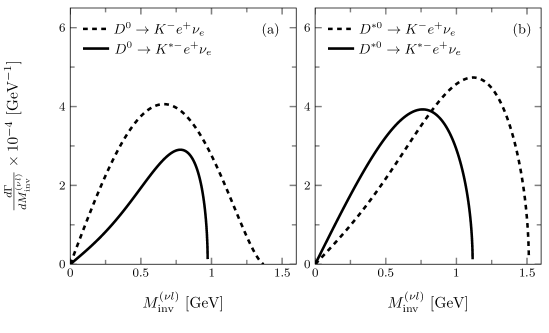
Figure 4: The differential width of semileptonic decay of $D$ or $D^{*}$ meson decay.

IV Conclusions

We have performed the angular momentum algebra in the evaluation of the weak matrix element in the semileptonic decays of $B^{(*)}$, $D^{(*)}$ mesons. The matrix elements of the weak current are evaluated in the rest frame of the $\nu l$ pair, which require spinors with finite (and large) momentum, and we obtain finally very simple expressions for the matrix elements involved and the sum over polarizations of their modulus squared. In terms of these analytical expressions we can give easy explanations for peculiarities in the invariant mass distributions and the ratios of rates for different reactions. By fixing the normalization of the theoretical rates to the experimental one of a reaction in the $B$ sector and another one in the $D$ sector, we can obtain the rate for the rest of the reactions. The agreement with experiment is good, with discrepancies for the production of $\tau$ leptons which we can trace to the different momentum transfers involved in the production of light $e$,$\mu$ leptons and $\tau$ lepton.

One of the output of the study is the prediction of decay rates for $B^{*}$ and $D^{*}$, which have been the object of discussion recently since they could be observed in future measurements of the LHCb collaboration. We justify that our predictions for these decay widths should be very accurate, which can be used in planning experiments to observe them in the future.

Appendix A Evaluation of the matrix elements

A.1 Evaluation of $M_{0}$

We start from the expression of $M_{0}$ in Eq. (19)

$$M_{0}=AA^{\prime}\delta_{ss^{\prime\prime}}\left\{1+BB^{\prime}p^{2}-(B+B^{\prime})\,p\,\sqrt{3}\,{\cal C}(\frac{1}{2}1\frac{1}{2};s,0,s)\right\}\,.$$ (41)

By looking at the spin third components of Fig. 1, we must combine $s,s^{\prime}$ to give $JM$ and $s^{\prime\prime},s^{\prime}$ to give $J^{\prime}M^{\prime}$. Thus we have

$$\sum_{s,s^{\prime},s^{\prime\prime}}{\cal C}\left(\frac{1}{2}\frac{1}{2}J;s,s^{\prime},M\right){\cal C}\left(\frac{1}{2}\frac{1}{2}J^{\prime};s^{\prime\prime},s^{\prime},M^{\prime}\right)AA^{\prime}\left\{1+BB^{\prime}p^{2}-(B+B^{\prime})p\sqrt{3}\,{\cal C}(\frac{1}{2}1\frac{1}{2};s,0,s)\right\}\delta_{ss^{\prime\prime}}\,.~{}~{}~{}~{}~{}~{}~{}$$ (42)

From here we conclude that $s+s^{\prime}=M$ and $s^{\prime\prime}+s^{\prime}=M^{\prime}$, and since $s^{\prime\prime}=s$ then $M=M^{\prime}$.

For the first two terms in Eq. (42) we get

$$\sum_{s}{\cal C}\left(\frac{1}{2}\frac{1}{2}J;s,M-s,M\right){\cal C}\left(\frac{1}{2}\frac{1}{2}J^{\prime};s,M-s,M\right)=\delta_{JJ^{\prime}}\,.$$ (43)

For the third term, we have a combination of three Clebsch-Gordan coefficients (CGC). We follow the angular momentum algebra of Rose rose and write

$${\cal C}\left(\frac{1}{2}\frac{1}{2}J;s,M-s,M\right) = (-1)^{\frac{1}{2}-s}\sqrt{\frac{2J+1}{2}}\ {\cal C}\left(J\frac{1}{2}\frac{1}{2};M,-s,M-s\right),$$

$${\cal C}\left(\frac{1}{2}\frac{1}{2}J^{\prime};s,M-s,M\right) = (-1)^{\frac{1}{2}+\frac{1}{2}-J^{\prime}}\ {\cal C}\left(\frac{1}{2}\frac{1}{2}J^{\prime};M-s,s,M\right),$$

$${\cal C}\left(\frac{1}{2}1\frac{1}{2};s,0,s\right) = (-1)^{\frac{1}{2}-s}\sqrt{\frac{2}{3}}\ {\cal C}\left(\frac{1}{2}\frac{1}{2}1;s,-s,0\right),$$ (44)

and then

$$\sum_{s}\mathcal{C}\left(\frac{1}{2}\frac{1}{2}J;s,M-s,M\right)\mathcal{C}\left(\frac{1}{2}\frac{1}{2}J^{\prime};s,M-s,M\right)\sqrt{3}\ \mathcal{C}\left(\frac{1}{2}1\frac{1}{2};s,0,s\right)$$ (45)

$$= (-1)^{1-J^{\prime}}\sqrt{2J+1}\ \mathcal{C}\left(J\frac{1}{2}\frac{1}{2};M,-s,M-s\right)\mathcal{C}\left(\frac{1}{2}\frac{1}{2}J^{\prime};M-s,s,M\right)\mathcal{C}\left(\frac{1}{2}\frac{1}{2}1;s,-s,0\right)$$

$$= (-1)^{1-J^{\prime}}\sqrt{2J+1}\sqrt{6}\ \mathcal{W}\left(J\frac{1}{2}J^{\prime}\frac{1}{2};\frac{1}{2}1\right)\mathcal{C}\left(J1J^{\prime};M,0,M\right)\,,$$

where $\mathcal{W}(\cdots)$ is a Racah coefficient.

Altogether

$$M_{0} = AA^{\prime}\bigg{\{}(1+BB^{\prime}p^{2})\delta_{MM^{\prime}}\,\delta_{JJ^{\prime}}$$ (46)

$$- \left.(B+B^{\prime})\ p\,\delta_{MM^{\prime}}\sqrt{6}\,\sqrt{2J+1}(-1)^{1-J^{\prime}}\mathcal{W}\left(J\frac{1}{2}J^{\prime}\frac{1}{2};\frac{1}{2}1\right)\mathcal{C}\left(J1J^{\prime};M,0,M\right)\right\}\,.$$

Calculating explicitly the Racah coefficient and the CGC, we find

• $J=0,J^{\prime}=0$

  $$M_{0}=AA^{\prime}(1+BB^{\prime}p^{2})\,\delta_{M0}\,\delta_{M^{\prime}0}\,.$$ (47)

• $J=0,J^{\prime}=1$

  $$M_{0}=-AA^{\prime}(B+B^{\prime})\,p\,\delta_{M0}\,\delta_{M^{\prime}0}\,.$$ (48)

• $J=1,J^{\prime}=0$

  $$M_{0}=-AA^{\prime}(B+B^{\prime})\,p\,\delta_{M0}\,\delta_{M^{\prime}0}\,.$$ (49)

• $J=1,J^{\prime}=1$

  $$M_{0}=AA^{\prime}\left\{(1+BB^{\prime}p^{2})\delta_{MM^{\prime}}-\sqrt{2}\,\delta_{MM^{\prime}}\,(B+B^{\prime})\,p\,\mathcal{C}(111;M,0,M)\right\}\,.$$ (50)

A.2 Evaluation of $N_{\mu}$

As seen in Eq. (21), we had $\gamma_{i}-\gamma_{i}\gamma_{5}$ written in spherical basis,

$$N_{\mu}=AA^{\prime}\left\{1-B\,p\,(-1)^{\frac{1}{2}-s}-B^{\prime}\,p\,(-1)^{\frac{1}{2}-s^{\prime\prime}}+BB^{\prime}p^{2}(-1)^{1-s-s^{\prime\prime}}\right\}\langle s^{\prime\prime}|{{\sigma}}_{\mu}|s\rangle\,,$$ (51)

and now we must project over $JM$ and $J^{\prime}M^{\prime}$. Thus, we get the combination

$$\sum_{s,s^{\prime},s^{\prime\prime}}\mathcal{C}\left(\frac{1}{2}\frac{1}{2}J;s,s^{\prime},M\right)\mathcal{C}\left(\frac{1}{2}\frac{1}{2}J^{\prime};s^{\prime\prime},s^{\prime},M^{\prime}\right)\sqrt{3}\ \mathcal{C}\left(\frac{1}{2}1\frac{1}{2};s,\mu,s^{\prime\prime}\right)\,,$$ (52)

which implies $s+s^{\prime}=M$ and $s^{\prime\prime}+s^{\prime}=M^{\prime}$, and then we get $s^{\prime\prime}+M-s=M^{\prime}$, and $s+\mu=s^{\prime\prime}$, $s+\mu+M-s=M^{\prime}$, so $\mu=M^{\prime}-M$.

Hence, we get the sum

$$S=\sum_{s}\mathcal{C}\left(\frac{1}{2}\frac{1}{2}J;s,M-s,M\right)\mathcal{C}\left(\frac{1}{2}\frac{1}{2}J^{\prime};M^{\prime}-M+s,M-s,M^{\prime}\right)$$

$$\times\sqrt{3}\ \mathcal{C}\left(\frac{1}{2}1\frac{1}{2};s,M^{\prime}-M,M^{\prime}-M+s\right)\,,$$ (53)

which goes with the term $"1"$ in the bracket of Eq. (51).

Permuting indices in the CGC, we have

$$\mathcal{C}\left(\frac{1}{2}\frac{1}{2}J;s,M-s,M\right) = (-1)^{\frac{1}{2}-s}\sqrt{\frac{2J+1}{2}}\ \mathcal{C}\left(J\frac{1}{2}\frac{1}{2};M,-s,M-s\right),$$

$$\mathcal{C}\left(\frac{1}{2}\frac{1}{2}J^{\prime};M^{\prime}-M+s,M-s,M^{\prime}\right) = (-1)^{1-J^{\prime}}\ \mathcal{C}\left(\frac{1}{2}\frac{1}{2}J^{\prime};M-s,M^{\prime}-M+s,M^{\prime}\right),$$

$$\mathcal{C}\left(\frac{1}{2}1\frac{1}{2};s,M^{\prime}-M,M^{\prime}-M+s\right) = (-1)^{\frac{1}{2}-s}\sqrt{\frac{2}{3}}\ \mathcal{C}\left(\frac{1}{2}\frac{1}{2}1;s,M-M^{\prime}-s,M-M^{\prime}\right),$$ (54)

$$= (-1)^{\frac{1}{2}-s}\sqrt{\frac{2}{3}}\mathcal{C}\left(\frac{1}{2}\frac{1}{2}1;-s,M^{\prime}-M+s,M^{\prime}-M\right)\,.~{}~{}~{}~{}~{}~{}~{}~{}~{}$$

Then the expression $S$ of Eq. (A.2) becomes

$$S = (-1)^{1-J^{\prime}}\sqrt{2J+1}\sum_{s}\mathcal{C}\left(J\frac{1}{2}\frac{1}{2};M,-s,M-s\right)$$ (55)

$$\times \mathcal{C}\left(\frac{1}{2}\frac{1}{2}J^{\prime};M-s,M^{\prime}-M+s,M^{\prime}\right)\mathcal{C}\left(\frac{1}{2}\frac{1}{2}1;-s,M^{\prime}-M+s,M^{\prime}-M\right)$$

$$= (-1)^{1-J^{\prime}}\sqrt{2J+1}\sqrt{6}\,\mathcal{W}\left(J\frac{1}{2}J^{\prime}\frac{1}{2};\frac{1}{2}1\right)\mathcal{C}\left(J1J^{\prime};M,M^{\prime}-M,M^{\prime}\right)\,.$$

The term $BB^{\prime}p^{2}(-1)^{1-s-s^{\prime\prime}}$ in Eq. (51) is easy, since $s+s^{\prime\prime}=M^{\prime}-M$ and we get the term $1+BB^{\prime}p^{2}(-1)^{M-M^{\prime}}$ times the expression Eq. (52).

Next we must evaluate the other two terms in Eq. (51) that have an extra phase,

$$(-1)^{\frac{1}{2}-s}\,;\qquad(-1)^{\frac{1}{2}-s^{\prime\prime}}=(-1)^{\frac{1}{2}+M-M^{\prime}-s}=(-1)^{\frac{1}{2}-s}\,(-1)^{M-M^{\prime}}$$ (56)

Since $(-1)^{M-M^{\prime}}$ is not affected by the $s$ sum, we only have one structure to calculate. Incorporating an extra phase in the sum is not trivial. To finally be able to reduce the sum over $s$ to Racah coefficients we write:

$$(-1)^{\frac{1}{2}-s}=\langle s|\sigma_{z}|s\rangle=\sqrt{3}\,\mathcal{C}(\frac{1}{2}1\frac{1}{2};s,0,s)\,.$$ (57)

We make the permutation

$$\mathcal{C}(\frac{1}{2}1\frac{1}{2};s,M^{\prime}-M,M^{\prime}-M+s)=(-1)\,\mathcal{C}(1\frac{1}{2}\frac{1}{2};M^{\prime}-M,s,M^{\prime}-M+s)\,,$$ (58)

and then write

$$\mathcal{C}(1\frac{1}{2}\frac{1}{2};M^{\prime}-M,s,M^{\prime}-M+s)\,\mathcal{C}(\frac{1}{2}\frac{1}{2}J^{\prime};M^{\prime}-M+s,M-s,M^{\prime})$$ (59)

$$= \sum_{j^{\prime\prime}}\sqrt{2(2j^{\prime\prime}+1)}\,\mathcal{W}(1\frac{1}{2}J^{\prime}\frac{1}{2};\frac{1}{2}j^{\prime\prime})\,\mathcal{C}(\frac{1}{2}\frac{1}{2}j^{\prime\prime};s,M-s,M)\,\mathcal{C}(1j^{\prime\prime}J^{\prime};M^{\prime}-M,M,M^{\prime})\,.~{}~{}~{}~{}~{}~{}$$

By means of the former equation we have decoupled two CGC depending on $s$ into one depending on $s$ and one independent of $s$. We can then combine the three $s$ dependent coefficients in term of a Racah and find

$$\sum_{s}\mathcal{C}(1\frac{1}{2}\frac{1}{2};0,s,s)\,\mathcal{C}(\frac{1}{2}\frac{1}{2}J;s,M-s,M)\,\mathcal{C}(\frac{1}{2}\frac{1}{2}j^{\prime\prime};s,M-s,M)$$ (60)

$$= [2(2j^{\prime\prime}+1)]^{\frac{1}{2}}W(1\frac{1}{2}J\frac{1}{2};\frac{1}{2}j^{\prime\prime})\,\mathcal{C}(1j^{\prime\prime}J;0,M,M)\,.$$

Summing all the terms, we obtain

$$N_{\mu} = AA^{\prime}\left\{\big{(}1+BB^{\prime}p^{2}(-1)^{M-M^{\prime}}\big{)}(-1)^{1-J^{\prime}}\sqrt{6}\,\sqrt{2J+1}\,\mathcal{W}(J\frac{1}{2}J^{\prime}\frac{1}{2};\frac{1}{2}1)\,\mathcal{C}(J1J^{\prime};M,M^{\prime}-M,M^{\prime})\right.$$ (61)

$$- 6\big{(}Bp+B^{\prime}p(-1)^{M-M^{\prime}}\big{)}\sum_{j^{\prime\prime}}(2j^{\prime\prime}+1)\,\mathcal{W}(1\frac{1}{2}J^{\prime}\frac{1}{2};\frac{1}{2}j^{\prime\prime})\,\mathcal{W}(1\frac{1}{2}J\frac{1}{2};\frac{1}{2}j^{\prime\prime})$$

$$\times \mathcal{C}(1j^{\prime\prime}J^{\prime};M^{\prime}-M,M,M^{\prime})\,\mathcal{C}(1j^{\prime\prime}J;0,M,M)\bigg{\}}\delta_{\mu,M^{\prime}-M}\,.$$

The sum over $j^{\prime\prime}$ runs over $0,1$ as one can see from the CGC $\mathcal{C}(\frac{1}{2}\frac{1}{2}j^{\prime\prime};s,M-s,M)$ of Eq. (60)

We can apply this formula to the particular cases and we find

• $J=0,J^{\prime}=0$

  $$N_{\mu}=-AA^{\prime}(B+B^{\prime})p\,\delta_{\mu 0}\,\delta_{M0}\,\delta_{M^{\prime}0}\,.$$ (62)

• $J=0,J^{\prime}=1$

  $$N_{\mu} = AA^{\prime}\left\{\big{(}1+BB^{\prime}p^{2}(-1)^{-M^{\prime}}\big{)}\right.$$ (63)

  $$+ \left.\sqrt{2}\,\big{(}Bp+B^{\prime}p(-1)^{-M^{\prime}}\big{)}\,\mathcal{C}(111;M^{\prime},0,M^{\prime})\right\}\,\delta_{\mu M^{\prime}}\,\delta_{M0}\,.$$

• $J=1,J^{\prime}=0$

  $$N_{\mu} = AA^{\prime}\left\{\big{(}1+BB^{\prime}p^{2}(-1)^{M}\big{)}(-1)^{-M}\right.$$ (64)

  $$- \left.\sqrt{2}\,(-1)^{M}\,\big{(}Bp+B^{\prime}p(-1)^{M}\big{)}\,\mathcal{C}(111;M,0,M)\right\}\,\delta_{\mu M}\,\delta_{M^{\prime}0}\,.$$

  The minus sign $-\sqrt{2}$ in Eq. (64) versus the $\sqrt{2}$ sign in Eq. (63) looks surprising but turns to be irrelevant in $\overline{\sum}\sum|t|^{2}$ because, as we shall show in next subsection, the two terms in Eqs. (63) or (64) do not interfere when summing over polarizations.

• $J=1,J^{\prime}=1$

  $$N_{\mu} = AA^{\prime}\left\{\big{(}1+BB^{\prime}p^{2}(-1)^{M-M^{\prime}}\big{)}\,\sqrt{2}\,\mathcal{C}(111;M,M^{\prime}-M,M^{\prime})\right.$$ (65)

  $$- \left.\big{(}Bp+B^{\prime}p(-1)^{M-M^{\prime}}\big{)}\,\delta_{M0}\right.$$

  $$- \left.2\big{(}Bp+B^{\prime}p(-1)^{M-M^{\prime}}\big{)}\,\mathcal{C}(111;M^{\prime}-M,M,M^{\prime})\,\mathcal{C}(111;0,M,M)\right\}\delta_{\mu,M^{\prime}-M}\,.~{}~{}~{}~{}~{}~{}~{}~{}~{}~{}$$

Appendix B Evaluation of $\overline{\sum}\sum|t|^{2}$

As shown in Eq. (30) we must evaluate

$$\overline{\sum}\sum\left|t\right|^{2}=L^{00}M_{0}~{}M^{*}_{0}+L^{0i}M_{0}~{}N^{*}_{i}+L^{i0}N_{i}~{}M_{0}^{*}+L^{ij}N_{i}~{}N_{j}^{*}\,,$$ (66)

by taking the expressions for $M_{0}$, $N_{\mu}$ obtained above and $L^{\alpha\beta}$ from Eq. (5)

$${L}^{\alpha\beta}=2~{}\frac{p_{\nu}^{\alpha}p_{l}^{\beta}+p_{l}^{\alpha}p_{\nu}^{\beta}-p_{\nu}\cdot p_{l}g^{\alpha\beta}-i\epsilon^{\rho\alpha\sigma\beta}p_{\nu\rho}p_{l\sigma}}{m_{\nu}m_{l}}\,.$$ (67)

We make the calculation for each $J,J^{\prime}$ combination, recalling that we are evaluating the matrix elements in the frame of the $\nu l$ at rest.

• $J=0,J^{\prime}=0$

  • First we evaluate the $L^{00}$ term of Eq. (66). The $\epsilon^{\rho\alpha\sigma\beta}$ term is zero since $\alpha=\beta=0$, By using Eq. (67) we find

    $$L^{00}=\frac{m^{2}_{l}}{m_{\nu}m_{l}}\frac{M_{\rm inv}^{2(\nu l)}-m^{2}_{l}}{M_{\rm inv}^{2(\nu l)}}\,,$$ (68)

    and then summing over the polarizations $M,M^{\prime}$ we find

    $$\overline{\sum_{M}}\sum_{M^{\prime}}L^{00}M_{0}M_{0}^{*}=\frac{m^{2}_{l}}{m_{\nu}m_{l}}\frac{M_{\rm inv}^{2(\nu l)}-m^{2}_{l}}{M_{\rm inv}^{2(\nu l)}}(AA^{\prime})^{2}(1+BB^{\prime}p^{2})^{2}\,.$$ (69)

  • The terms from $L^{0i}$,$L^{i0}$ are zero in the sum over polarizations and integration over phase space. Indeed, since ${\bm{p}}_{\nu}=-{\bm{p}}_{l}$ in the $\nu l$ rest frame.

    $$p_{l}^{0}p_{\nu}^{i}+p_{\nu}^{0}p_{l}^{i}=p_{l}^{0}p_{\nu}^{i}-p_{\nu}^{0}p_{\nu}^{i}\,,$$ (70)

    and

    $$\int d\Omega\,p_{\nu i}\rightarrow\int d\Omega\,Y_{1\mu}({\widehat{\bm{p}}}_{\nu})=0\,.$$ (71)

    The $\epsilon^{\rho\alpha\sigma\beta}$ term is now $\epsilon^{\rho 0\sigma i}$ and

    $$\epsilon^{\rho 0\sigma i}p_{\nu\rho}p_{l\sigma}=-\epsilon^{\rho\sigma i}p_{\nu\rho}p_{l\sigma}=\epsilon^{\rho\sigma i}p_{\nu\rho}p_{\nu\sigma}=0\,.$$ (72)

    A similar approach can be used for the $\epsilon$ term in all the other cases and one can show that it always vanishes.

  • For the term from $L^{ij}N_{i}N_{j}^{*}$, this evaluation is made easy recalling that we take ${\bm{p}}$ in the $z$ direction and we found in Eq. (62) that $N_{\mu}$ is proportional to $\delta_{\mu 0}$ $(\mu=0,i=3)$. Hence we get

    $$L^{33}N_{3}N_{3}^{*}=L^{33}N_{0}N_{0}^{*}\,,$$ (73)

    and

    $$L^{33} = \frac{2}{m_{\nu}m_{l}}\left\{2\widetilde{p}_{l3}\widetilde{p}_{\nu 3}+\delta_{33}\widetilde{p}_{l}\cdot\widetilde{p}_{\nu}\right\}$$

    $$= \frac{2}{m_{\nu}m_{l}}\left\{-2\widetilde{p}_{\nu 3}\widetilde{p}_{\nu 3}+\widetilde{E}_{\nu}\widetilde{E}_{l}+\widetilde{p}^{2}_{\nu}\right\}$$

    $$= \frac{2}{m_{\nu}m_{l}}\left\{-\frac{2}{3}\widetilde{p}^{2}_{\nu}+\widetilde{E}_{\nu}\widetilde{E}_{l}+\widetilde{p}^{2}_{\nu}\right\}\,,$$

    where the last step uses the fact $\widetilde{p}_{\nu i}\widetilde{p}_{\nu j}$ becomes $\frac{1}{3}\delta_{ij}\widetilde{p}^{2}_{\nu}$ upon integration over $d\Omega({\widehat{\bm{p}}}_{\nu})$ in the phase space.

    Then we find

    $$\overline{\sum_{M}}\sum_{M^{\prime}}L^{ij}N_{i}N_{j}^{*}=\frac{2}{m_{\nu}m_{l}}\big{[}\widetilde{E}_{\nu}\widetilde{E}_{l}+\frac{1}{3}\widetilde{p}_{\nu}^{2}\big{]}(AA^{\prime})^{2}(B+B^{\prime})^{2}p^{2},$$ (75)

    and altogether

    $$\overline{\sum}\sum|t|^{2} = \frac{(AA^{\prime})^{2}}{m_{\nu}m_{l}}\left\{\frac{m^{2}_{l}(M_{\rm inv}^{2(\nu l)}-m^{2}_{l})}{M_{\rm inv}^{2(\nu l)}}(1+BB^{\prime}p^{2})^{2}\right.$$

    $$+ \left.2(\widetilde{E}_{\nu}\widetilde{E}_{l}+\frac{1}{3}\widetilde{p}_{\nu}^{2})(B+B^{\prime})^{2}p^{2}\right\}\,.$$

• $J=0,J^{\prime}=1$

  • Using Eqs. (48) and (68), we find

    $$\overline{\sum}\sum L^{00}M_{0}M_{0}^{*}=\frac{m^{2}_{l}}{m_{\nu}m_{l}}\frac{M_{\rm inv}^{2(\nu l)}-m^{2}_{l}}{M_{\rm inv}^{2(\nu l)}}(AA^{\prime})^{2}(B+B^{\prime})^{2}p^{2}\,.$$ (77)

  • The $\epsilon$ term and $L^{0i}$ also vanish when integrating over $d\Omega({\widehat{\bm{p}}}_{\nu})$.

  • For the term from $L^{ij}N_{i}N_{j}^{*}$ we need Eq. (63) and

    $$L^{ij}=\frac{2}{m_{\nu}m_{l}}\left\{-2p_{\nu}^{i}p_{\nu}^{j}+\delta_{ij}(p_{\nu}\cdot p_{l})\right\}\,.$$ (78)

    We now write in spherical basis

    $$\sum_{i}p_{\nu i}N_{i} = \sum_{\alpha}(-1)^{\alpha}p_{\nu\alpha}N_{-\alpha}\,,$$ (79)

    $$\sum_{i}p_{\nu i}N_{i}^{*} = \sum_{\beta}p_{\nu\beta}N_{\beta}^{*}\,.$$

    One evaluates first the $\widetilde{p}_{\nu i}\widetilde{p}_{\nu j}$ term, writes

    $$\widetilde{p}_{\nu\alpha}=\sqrt{\frac{4\pi}{3}}\tilde{p}_{\nu}Y_{1\alpha}({\widehat{\bm{p}}}_{\nu})\,,$$ (80)

    and use that

    $$\int Y_{1\alpha}({\widehat{\bm{p}}}_{\nu})Y_{1\beta}({\widehat{\bm{p}}}_{\nu})d\Omega({\widehat{\bm{p}}}_{\nu})=\delta_{\alpha\beta}\,,$$ (81)

    and we get

    $$\overline{\sum_{M}}\sum_{M^{\prime}}-\frac{4}{m_{\nu}m_{l}}\tilde{p}^{i}_{\nu}\tilde{p}^{j}_{\nu}N_{i}N_{j}^{*}=-\frac{4}{m_{\nu}m_{l}}(AA^{\prime})^{2}\frac{1}{3}\widetilde{p}^{2}_{\nu}\,\delta_{M0}$$

    $$\times \left\{\big{(}1+BB^{\prime}p^{2}(-1)^{-M^{\prime}}\big{)}+\sqrt{2}\,\big{(}Bp+B^{\prime}p(-1)^{-M^{\prime}}\big{)}\,\mathcal{C}(111;M^{\prime},0,M^{\prime})\right\}^{2}\,.$$

    And explicit evaluation of the square of the bracket and the sum over $M,M^{\prime}$ gives at the end

    $$\overline{\sum_{M}}\sum_{M^{\prime}}-\frac{4}{m_{\nu}m_{l}}\tilde{p}^{i}_{\nu}\tilde{p}^{j}_{\nu}N_{i}N_{j}^{*}$$

    $$= -\frac{4}{m_{\nu}m_{l}}(AA^{\prime})^{2}\frac{1}{3}\widetilde{p}^{2}_{\nu}\left\{3-6BB^{\prime}p^{2}+2(B^{2}+B^{\prime 2})p^{2}+3(BB^{\prime}p^{2})^{2}\right\}\,.$$

    The term $\delta_{ij}(p_{\nu}\cdot p_{\ell})N_{i}N_{j}^{*}$ is evaluated in the same way and we find

    $$\overline{\sum_{M}}\sum_{M^{\prime}}L^{ij}N_{i}N_{j}^{*}$$

    $$= \frac{2}{m_{\nu}m_{l}}(AA^{\prime})^{2}\big{(}\widetilde{E}_{\nu}\widetilde{E}_{l}+\frac{1}{3}\tilde{p}_{\nu}^{2}\big{)}\left\{3-6BB^{\prime}p^{2}+2(B^{2}+B^{\prime 2})p^{2}+3(BB^{\prime}p^{2})^{2}\right\}\,,$$

    and summing the $L^{00}M_{0}M_{0}^{*}$ contribution we obtain at the end

    $$\overline{\sum_{M}}\sum_{M^{\prime}}|t|^{2} = \frac{(AA^{\prime})^{2}}{m_{\nu}m_{l}}\left\{2\big{(}\widetilde{E}_{\nu}\widetilde{E}_{l}+\frac{1}{3}\tilde{p}_{\nu}^{2}\big{)}\left[3-6BB^{\prime}p^{2}+\right.\right.$$

    $$\left.\left.2(B^{2}+B^{\prime 2})p^{2}+3(BB^{\prime}p^{2})^{2}\right]+\frac{m^{2}_{l}(M_{\rm inv}^{2(\nu l)}-m^{2}_{l})}{M_{\rm inv}^{2(\nu l)}}(B+B^{\prime})^{2}p^{2}\right\}\,.~{}~{}~{}~{}~{}~{}$$

• $J=1,J^{\prime}=0$
  We obtain the same result as before, but must multiply by $\frac{1}{3}$ to take into account the average over the initial polarizations.
  

• $J=1,J^{\prime}=1$

  • $L^{00}M_{0}M^{*}_{0}$ term
    We need the expression of Eq. (50). We can see that in $M_{0}M_{0}^{*}$ we have terms like

    $$\sum_{M}{\cal C}(111;M,0,M) = 0\,,$$

    $$\sum_{M}{\cal C}(111;M,0,M)\,{\cal C}(1,1,1;M,0,M) = \frac{1}{2}+0+\frac{1}{2}=1\,,$$ (86)

    then

    $$\overline{\sum_{M}}\sum_{M^{\prime}}L^{00}M_{0}M_{0}^{*}=(AA^{\prime})^{2}\frac{m^{2}_{l}}{m_{\nu}m_{l}}\frac{M_{\rm inv}^{2(\nu l)}-m^{2}_{l}}{M_{\rm inv}^{2(\nu l)}}\left\{(1+BB^{\prime}p^{2})^{2}+\frac{2}{3}(B+B^{\prime})^{2}p^{2}\right\}\,.~{}~{}~{}~{}~{}~{}~{}~{}~{}~{}$$ (87)

  • For the same reasons as before $L^{0i}M_{0}N_{i}^{*}$,$L^{i0}N_{i}M_{0}^{*}$ vanish in the integration over phase space.

  • $L^{ij}N_{i}N_{j}^{*}$ term
    $L^{ij}$ is given by Eq. (78), proceeding as we have done before. The extra CGC in this term are easily handled since $\mathcal{C}(111;0,0,0)$ and the other coefficients are all $\frac{1}{\sqrt{2}}$ except for a phase. We need the expression of Eq. (65) and we can easily see that in the sum over $M,M^{\prime}$ the three terms of this equation do not interfere. An explicit bookkeeping and some algebra allows as to write finally

    $$\overline{\sum_{M}}\sum_{M^{\prime}}|t|^{2} = \frac{1}{3}\,\frac{(AA^{\prime})^{2}}{m_{\nu}m_{l}}\left\{\frac{3\,m^{2}_{l}(M_{\rm inv}^{2(\nu l)}-m^{2}_{l})}{M_{\rm inv}^{2(\nu l)}}\left[(1+BB^{\prime}p^{2})^{2}+\frac{2}{3}(B+B^{\prime})^{2}p^{2}\right]\right.$$ (88)

    $$+ \left.2\left(\widetilde{E}_{\nu}\widetilde{E}_{l}+\frac{1}{3}\widetilde{p}^{2}_{\nu}\right)\left[6+7(B^{2}+B^{\prime 2})p^{2}-4BB^{\prime}p^{2}+6(BB^{\prime}p^{2})^{2}\right]\right\}\,.~{}~{}~{}~{}~{}~{}~{}~{}$$

References

- (1) T. E. Browder and K. Honscheid, Prog. Part. Nucl. Phys. 35, 81 (1995).
- (2) N. Isgur and M. B. Wise, Phys. Lett. B 232, 113 (1989).
- (3) N. Isgur, D. Scora, B. Grinstein and M. B. Wise, Phys. Rev. D 39, 799 (1989).
- (4) M. Wirbel, Prog. Part. Nucl. Phys. 21, 33 (1988).
- (5) M. Neubert and B. Stech, Adv. Ser. Direct. High Energy Phys. 15, 294 (1998).
- (6) G. Ecker, Prog. Part. Nucl. Phys. 35, 1 (1995).
- (7) M. Neubert, Int. J. Mod. Phys. A 11, 4173 (1996).
- (8) M. Antonelli et al., Phys. Rept. 494, 197 (2010).
- (9) S. Fajfer, J.F. Kamenik, and I. Niandi, Phys. Rev. D 85, 094025 (2012).
- (10) Xiao-Gang He, German Valencia, Phys. Lett. B 779, 52 (2018).
- (11) C. Albertus, E. Hernndez, J. Nieves, and J. M. Verde-Velasco, Phys. Rev. D. 71, 113006 (2005).
- (12) Tianhong Wang, Yue Jiang, Tian Zhou, Xiao-Ze Tan, and Guo-Li Wang, arXiv:1804.06545 [hep-ph].
- (13) Q. Chang, J. Zhu, X. L. Wang, J. F. Sun, and Y. L. Yang, Nucl. Phys. B 909, 921 (2016).
- (14) Matthias Neubert, Phys. Rept. 245, 259 (1994).
- (15) A. V. Manohar and M. B. Wise, Camb. Monogr. Part. Phys. Nucl. Phys. Cosmol. 10, 1 (2000).
- (16) Fernando S. Navarra, Marina Nielsen, Eulogio Oset, and Takayasu Sekihara, Phys. Rev. D. 92, 014031 (2015).
- (17) F. Mandl and G. Shaw, Quantum Field Theory, John Wiley Sons, (1984).
- (18) C. Itzykson and J. B. Zuber, Quantum Field Theory, Mecraw-Hill, 1980.
- (19) C. Patrignani et al. (Particle Data Group). Chin. Phys. C 40, 100001 (2016).
- (20) Y. Amhis et al. Heavy Flavor Averaging Group (HFLAV), Eur. Phys. J. C 77, 895 (2017).
- (21) R. Aaij et al. (LHCb Collaboration), Phys. Rev. D 97, 072013 (2018).
- (22) Jon A. Bailey et al. (Fermilab Lattice and MILC Collaborations), Phys. Rev. D 92, 034506 (2015).
- (23) Heechang Na et al. (HPQCD Collaboration), Phys. Rev. D 92, 054510 (2015); Erratum Phys. Rev. D 93, 119906 (2016).
- (24) J. E. Chavez-Saab, Genaro Toledo, arXiv:1806.06997
- (25) R. Aaij et al. (LHCb Collaboration), Phys. Rev. Lett. 120, 121801 (2018).
- (26) A. Yu. Anisimov, I. M. Narodetskii, C. Semay, B. Silvestre-Brac, Phys. Lett. B 452, 129 (1999).
- (27) V. V. Kiselev, arXiv:hep-ph/0211021
- (28) Mikhail A. Ivanov, Jürgen G. Körner, and Pietro Santorelli, Phys. Rev. D 73, 054024 (2006).
- (29) E. Hernndez, J. Nieves, and J. M. Verde-Velasco, Phys. Rev. D 74, 074008 (2006).
- (30) J. M. Zhang and G. L. Wang, Chin. Phys. Lett. 27, 051301 (2010).
- (31) M. E. Rose, Elementary Theory of Angular Momentum, John Wiley Sons, 1957.
- (32) D. Ebert, R. N. Faustov, and V. O. Galkin, Eur. Phys. J. C 71, 1825 (2011).
- (33) W. H. Liang and E. Oset, arXiv:1804.00938 [hep-ph] [Eur. Phys. J. C in print).
- (34) L. R. Dai, R. Pavao, S. Sakai and E. Oset, arXiv:1805.04573 [hep-ph].