A chemical and kinematical analysis of the intermediate-age open cluster IC 166 from APOGEE and Gaia DR2

Abstract

IC 166 is an intermediate-age open cluster ($\sim 1$ Gyr) which lies in the transition zone of the metallicity gradient in the outer disc. Its location, combined with our very limited knowledge of its salient features, make it an interesting object of study. We present the first high-resolution spectroscopic and precise kinematical analysis of IC 166, which lies in the outer disc with $R_{GC}\sim 12.7$ kpc. High resolution H-band spectra were analyzed using observations from the SDSS-IV Apache Point Observatory Galactic Evolution Experiment (APOGEE) survey. We made use of the Brussels Automatic Stellar Parameter (BACCHUS) code to provide chemical abundances based on a line-by-line approach for up to eight chemical elements (Mg, Si, Ca, Ti, Al, K, Mn and Fe). The $\alpha-$element (Mg, Si, Ca and whenever available Ti) abundances, and their trends with Fe abundances have been analysed for a total of 13 high-likelihood cluster members. No significant abundance scatter was found in any of the chemical species studied. Combining the positional, heliocentric distance, and kinematic information we derive, for the first time, the probable orbit of IC 166 within a Galactic model including a rotating boxy bar, and found that it is likely that IC 166 formed in the Galactic disc, supporting its nature as an unremarkable Galactic open cluster with an orbit bound to the Galactic plane.

=1 Co-authors and affiliations can be found after the acknowledgements

1 Introduction

Galactic open clusters (OCs) have a wide age range, from 0 to almost 10 Gyr, and they are spread throughout the Galactic disc; therefore, they are widely used to characterize the properties of the Galactic disc, such as the morphology of the spiral arms of the Milky Way (MW) (Bonatto et al., 2006; van den Bergh, 2006; Vázquez et al., 2008), the stellar metallicity gradient (e.g., Cunha et al. 2016; Jacobson et al. 2016; Frinchaboy et al. 2013; Geisler et al. 1997; Janes 1979), the age-metallicity relation in the Galactic disc (Magrini et al., 2009; Salaris et al., 2004; Carraro & Chiosi, 1994; Carraro et al., 1998), and the Galactic disc star formation history (de la Fuente Marcos & de la Fuente Marcos, 2004). OCs are thus crucial in developing a more comprehensive understanding of the Galactic disc.

OCs are generally considered to be archetypal examples of a simple stellar population (Deng & Xin, 2007), because individual member stars of each OC are essentially homogeneous, both in age, dynamically (similar radial velocities and proper motions) and chemically (similar chemical patterns), greatly facilitating our ability to derive global cluster parameters from studying limited samples of stars. However, possible small inhomogeneous chemical patterns in OCs have been recently suggested, though only at the 0.02 dex level (e.g. Hyades; Liu et al. 2016).

IC 166 ($l=130.071^{\circ}$, $b=-0.189^{\circ}$) is an intermediate-age OC ($\sim$1.0 Gyr, Vallenari et al. 2000; Subramaniam & Bhatt 2007) located in the outer part of the Galactic disc (R${}_{GC}\approx$13 kpc). Previous literature studies of this cluster used mainly photometric and low-resolution spectroscopic data. Detailed photometric studies were carried out by Subramaniam & Bhatt (2007); Vallenari et al. (2000) and Burkhead (1969) in order to estimate its age, extinction, and distance. In addition, Dias et al. (2014, 2002); Loktin & Beshenov (2003) and Twarog et al. (1997) have derived proper motions in the IC 166 field. Friel & Janes (1993) and Friel et al. (1989) have estimated the radial velocity and metallicity of IC 166 from low-resolution spectroscopic data. In this work, we will for the first time provide an extensive, detailed investigation of its chemical abundances as well as its orbital parameters.

OCs are continuously influenced by destructive effects such as (1) evaporation (Moyano Loyola & Hurley, 2013), where some members reach the escape velocity after intracluster stellar encounters with other members, and/or via interaction with the Galactic tidal field, and (2) close encounters with giant interstellar clouds (Gieles & Renaud, 2016). Interactions with giant molecular clouds along their orbit in the Galactic disc have a high probability to eventually disrupt star clusters (Lamers et al., 2005; Gieles et al., 2006; Lamers & Gieles, 2006). These effects can lead to the dissolution of a typical open cluster in $\sim$10⁸ years (Friel, 2013). Thus, intermediate-age and old OCs ($\geq$1.0 Gyr) are rare by nature and are of great interest (Friel et al., 2014; Donati et al., 2014; Magrini et al., 2015; Tang et al., 2017). As these effects are generally less severe in the outer disc, OCs there have a higher chance of survival, providing a great opportunity to study this part of the Galaxy both chemically and dynamically. Moreover, IC 166 is located close to the region where a break in the metallicity gradient is suggested (between 10 kpc and 13 kpc from the Galactic center; Frinchaboy et al. 2013; Yong et al. 2012; Reddy et al. 2016). Accurate determination of the cluster’s metallicity is helpful to constrain the nature of this possible break.

Large scale multi-object spectroscopic surveys, such as the Apache Point Observatory Galactic Evolution Experiment (APOGEE: Majewski et al. 2017) provide a unique opportunity to study a wide gamut of light-/heavy-elements in the H-band in hundreds of thousands of stars in a homogeneous way (García Pérez et al., 2016; Hasselquist et al., 2016; Cunha et al., 2017). In this work, we provide an independent abundance determination of several chemical species in the open cluster IC 166 using the Brussels Automatic Code for Characterizing High accUracy Spectra (BACCHUS: Masseron et al. 2016), and compare them with the Apogee Stellar Parameter and Chemical Abundances Pipeline (ASPCAP: García Pérez et al. 2016).

This paper is organized as follows. Cluster membership selection is described in Section 2. In Section 3 we determine the atmospheric parameters for our selected members. In Section 4 we present our derived chemical abundances. A detailed description of the orbital elements is given in Section 5. We present our conclusions in Section 6.

2 Target Selection

The Apache Point Observatory Galactic Evolution Experiment (APOGEE: Majewski et al., 2017) is one of the projects operating as part of the Sloan Digital Sky Survey IV (Abolfathi et al., 2018; Blanton et al., 2017), aiming to characterize the Milky Way Galaxy’s formation and evolution through a precise, systematic and large scale kinematic and chemical study. The APOGEE instrument is a near-infrared ($\lambda=1.51-1.70$ $\mu$m) high resolution ($R\approx 22,500$) multi-object spectrograph (Wilson et al., 2012) mounted at the SDSS 2.5 m telescope (Gunn et al., 2006), with a copy now operating in the South at Las Campanas Observatory –the 2.5-meter Irénée du Pont telescope. The APOGEE survey has observed more than 270,000 stars across all of the main components of the Milky Way (Zasowski et al., 2013, 2017), achieving a typical spectral signal to noise ratio (S/N) $>$100 per pixel. The latest data release (DR14: Abolfathi et al., 2018) includes all of the APOGEE-1 data and APOGEE data taken between July 2014 and July 2016. A number of candidate member stars of the open cluster IC 166 were observed by the APOGEE survey, and their spectra were released for the first time as part of the DR14 (Abolfathi et al., 2018).

We selected a sample of potential stellar members for IC 166 using the following high quality control cuts:

• Spatial Location: We focus on stars that are located inside half of the tidal radius ($r_{t}/2$), where $r_{t}=$ 35.19 $\pm$ 6.10 pc (Kharchenko et al., 2012). This can minimize Galactic foreground stars. Figure 1 shows the spatial distribution of 21 highest likelihood cluster members inside half of the tidal radius, highlighted with red dots, for our final sample of likely cluster members. Stars with projected distances from the center larger than half of the tidal radius were removed, in order to obtain a cleaner sample, relatively uncontaminated by disc stars.

• Radial Velocity and Metallicity: We further selected member stars using their radial velocities (RVs). Figure 2 shows the RV versus [Fe/H] distribution of the stars in the APOGEE observation field of IC 166. Clearly, twenty out of twenty-one likely cluster members that we selected using only spatial information show a RV peak around $-40$ km s^-1, except one with much lower RV ($\approx-96$ km s^-1). The other 20 cluster members show a mean RV of $-40.50\pm 1.66$ km s^-1. Applying a 3$\sigma$ limit, we excluded stars outside of $-40.50\pm 3\times 1.66$ km s^-1 (gray region in Figure 2). Twenty stars were selected as likely members. After the spatial location and RV selection, their membership status is further scrutinized by filtering out all stars failing to meet the metallicity criteria. We adopt the calibrated metallicity from DR14 APOGEE/ASPCAP as a first guess in order to derive a cleaner sample of cluster stars. We identified a metallicity peak at $-$0.06 dex; thus stars with metallicities differing by more than 0.03 dex from this mean were removed. Fifteen stars were left as likely members.

• CMD Location: The left panel of Figure 3 shows the 2MASS (K_s, J-K_s) Color-Magnitude diagram, for all stars lying inside one half of the tidal radius. Our selected APOGEE sample clearly lies near the red clump, consistent with the red clump observed in the $T_{\rm eff}$ vs. log(g) plane (right panel of Figure 3). Interestingly, Vallenari et al. (2000) also reported a clear red clump in IC 166, but did not find evidence of RGB stars. Two out of the fifteen stars selected previously were located away from the red clump of IC 166. These stars were also removed from further consideration, although isochrones indicate they could well be upper RGB members. The isochrones shown in Figure 3 were selected from PARSEC (Bressan et al., 2012) for [Fe/H] =-0.06 dex and ages (0.8, 1.0 and 1.2 Gyr; Vallenari et al. 2000; Subramaniam & Bhatt 2007) to match the metallicity and age reported for this cluster. The candidates are in good agreement with the selected isochrones. The PARSEC isochrones used have been fitted by eye to the luminosity and colour of the red clump stars. There is a small discrepancy in the location of de-reddened red clump stars found using the optical photometry and the T_eff vs. log(g) diagram.

Lastly, we examine the newly-measured proper motions from Gaia DR2 (Gaia Collaboration et al., 2018; Lindegren et al., 2018) of the APOGEE/IC 166 candidates. Figure 5 shows the proper motion diagram for IC 166. The dashed lines show the estimated mean proper motion value for IC 166. Gaia DR2 reveals that the selected stars in this study exhibit similar proper motions to each other, with a relatively small spread ($<$ 0.2 mas yr^-1; see Figure 5), which are good enough for a precise orbit predictions of IC 166.

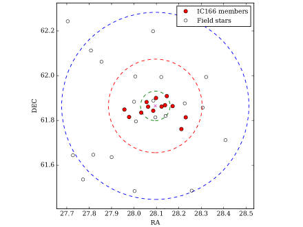
Figure 1: On-sky distribution of the 13 highest likelihood cluster members analyzed in this work (red symbols) and within 17.6 arcmin (half of the tidal radius) of the center (red dashed line). The inner ”x” symbol is the center of the cluster. Indicated with black open circles are field stars that were also observed by APOGEE. The large blue dashed circle shows the tidal radius of the cluster (35.19 arcmin), while the inner green dashed circle shows the core radius of the cluster.

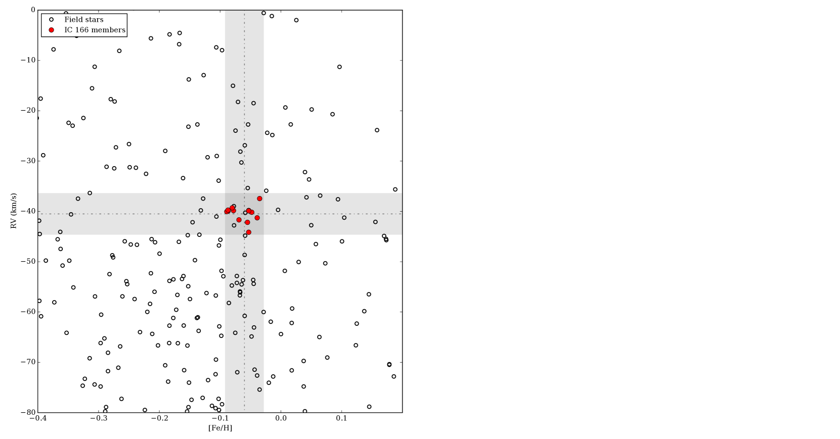
Figure 2: The APOGEE/DR14 RV vs. metallicity of stars in the field of the cluster (gray open circles) and our final sample (red dots). The gray regions show the upper and lower limits for the membership selection described in the text. The dotted lines show the mean RV and [Fe/H] of our final sample.

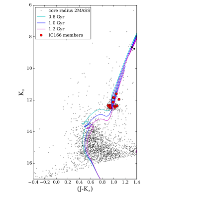
Figure 3: CMD of IC 166 using J and K_s magnitudes. Small gray points represent stars observed by 2MASS inside of the $r_{core}$. Red dots represent our potential members observed by APOGEE and black dots the two stars not passing our high quality cuts (see text). Isochrones for 0.8 Gyr (sky-blue line), 1.0 Gyr (blue line) and 1.2 Gyr (magenta line) from PARSEC are also plotted.

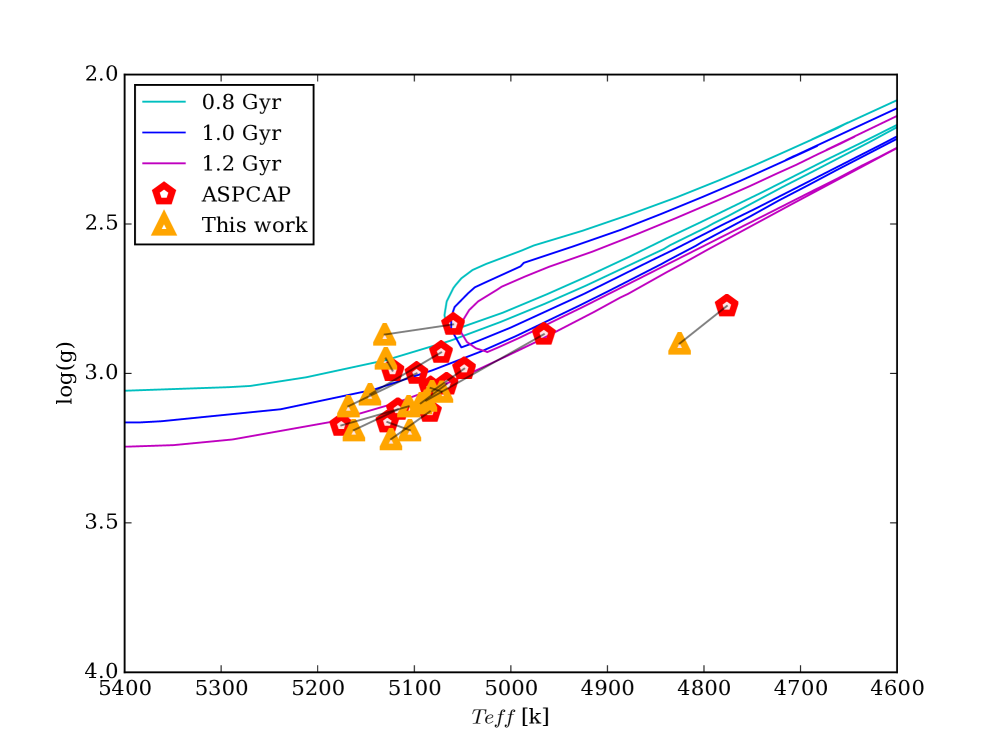
Figure 4: Log(g)-$T_{\rm eff}$ plane: Stellar parameters from ASPCAP and this work are represented with red pentagons and orange triangles, respective. Isochrones follow the same description as the Figure 3. Black lines show which points refer to the same stars.

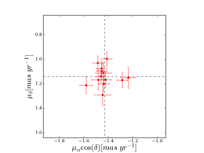
Figure 5: Proper motion diagram for the stars selected as members of IC 166 from Gaia DR2. The dashed lines are the mean proper motion estimated for IC 166 (see text).

Table 1 shows the basic parameters of the stars which satisfy all the criteria previously mentioned, where raw $T_{\rm eff}$ and log(g) have been considered. These 13 stars will be considered as likely members of IC 166 and constitute our final cluster sample.

Table 1: Summary table of likely members of IC 166.

Apogee ID	Tag	RA	DEC	J	K	% a
2M01514975+6150556	Star #1	27.957296	61.848778	13.417	12.360	…
2M01515473+6148552	Star #2	27.978044	61.815334	13.403	12.393	95
2M01520770+6150058	Star #3	28.032106	61.834946	13.446	12.503	96
2M01521347+6152558	Star #4	28.056156	61.882183	13.487	12.462	…
2M01521509+6151407	Star #5	28.062883	61.861309	13.118	12.129	84
2M01522060+6150364	Star #6	28.085842	61.843445	12.835	11.845	95
2M01522357+6154011	Star #7	28.098241	61.900307	13.262	12.327	96
2M01522953+6151427	Star #8	28.123055	61.861885	12.649	11.603	…
2M01523324+6152050	Star #9	28.138523	61.868073	13.244	12.343	63
2M01523513+6154318	Star #10	28.146393	61.908844	13.326	12.409	…
2M01524136+6151507	Star #11	28.172348	61.864094	13.385	12.445	93
2M01525074+6145411	Star #12	28.211422	61.76144	13.048	11.956	…
2M01525543+6148504	Star #13	28.230962	61.814007	12.847	11.844	…

^a Membership probability from Dias et al. (2014)

3 Atmospheric parameters and abundance determinations

For the stars observed with APOGEE and identified as members in §2, atmospheric parameters (T_eff, log g, [M/H] and $\xi$) were determined using the code FERRE (Allende Prieto et al., 2006) that compares theoretical spectra computed from MARCS atmosphere models (Gustafsson et al., 2008; Zamora et al., 2015) using the entire wavelength range, and minimizes the difference with the observed spectrum via a $\chi^{2}$ minimization. Our synthetic spectra were based on 1D Local Thermodynamic Equilibrium (LTE) model atmospheres calculated with MARCS (Gustafsson et al., 2008). The derived atmospheric parameters are listed in Table 2.

It is important to note that we chose not to estimate the T${\rm eff}$ values from any empirical color-temperature relation; this would be highly uncertain due to relatively large and likely differential reddening along the line-of-sight to IC 166, $E(B-V)\approx$ 0.80 (Subramaniam & Bhatt, 2007).

Figure 4 displays the main stellar parameters determined from FERRE/MARCS against those computed from ASPCAP/KURUCZ (raw values), overplotted on the PARSEC isochrones (Bressan et al., 2012) with ages of 0.8, 1.0 and 1.2 Gyr. We notice that the raw (not post-calibrated) stellar parameters obtained via ASPCAP/KURUCZ are in fairly good agreement with the stellar parameters derived in this study using FERRE/MARCS. After deriving the stellar parameters we used the code BACCHUS (see Masseron et al., 2016; Hawkins et al., 2016) to fit the spectral features of the atomic lines for up to eight chemical elements (Fe, Mg, Al, Si, Ca, Ti, K, and Mn). We did not analyze OH, CN, and CO, because these molecular lines are weak in the typical range of T_eff and metallicity for the stars studied in this work, and such an analysis would lead to unreliable abundance results for carbon, nitrogen and oxygen. The line list used in this work is the latest internal DR14 atomic/molecular line list (linelist.20150714: Holtzmman et al. in preparation). For each atomic line, the abundance determination proceeded in the same fashion as described in Hawkins et al. (2016), i.e., we computed spectrum synthesis, using the full set of atomic lines to find the local continuum level via a linear fit; the local S/N was estimated and the abundances were then determined by comparing the observed spectrum with the set of convolved synthetic spectra for different abundances. The BACCHUS code determines line-by-line abundances via four different approaches: (i) line-profile fitting; (ii) core line intensity comparison; (iii) global goodness-of-fit estimate ($\chi^{2}$); and (iv) equivalent width comparison, with each diagnostic yielding validation flags used to reject or accept a line, keeping the best fit abundance (see, e.g., Hawkins et al., 2016). Following the suggestion by Hawkins et al. (2016); Fernández-Trincado et al. (2018) we adopted the $\chi^{2}$ diagnostic as the most robust abundance determination. The selected atomic lines were then visually inspected to ensure that the spectral fits were adequate. The spectral regions used in our analysis are listed in Table A1.

Table 2: Stellar parameters obtained from FERRE/MARCS.

This work					ASPCAP
ID	T${\rm eff}$	log(g)	[Fe/H]	$\xi$	T${\rm eff}$	log(g)	[Fe/H]	$\xi$
star #1	5070	3.06	-0.01	1.32	5085	3.05	-0.05	1.70
star #2	5080	3.06	-0.08	1.25	5050	3.00	-0.08	1.50
star #3	5130	2.95	-0.05	0.93	5120	3.00	-0.09	1.10
star #4	5095	3.10	-0.05	1.16	5065	3.05	-0.05	1.60
star #5	5145	3.07	-0.04	1.55	5070	2.95	-0.05	1.70
star #6	5105	3.19	-0.05	1.06	5130	3.15	-0.03	1.50
star #7	5170	3.11	-0.10	1.42	5100	3.00	-0.09	1.60
star #8	4825	2.90	-0.07	1.19	4775	2.75	-0.04	1.50
star #9	5105	3.11	-0.11	1.24	5175	3.15	-0.05	1.60
star #10	5165	3.19	-0.10	1.28	5115	3.10	-0.08	1.70
star #11	5125	3.22	-0.06	1.08	5085	3.15	-0.05	1.45
star #12	5130	2.87	-0.06	1.69	5060	2.85	-0.09	1.70
star #13	5090	3.09	-0.05	1.42	4965	2.85	-0.07	1.70

Table 3: IC 166 Data Sample from Gaia DR2 and APOGEE.

APOGEEID	$\alpha$	$\delta$	Parallax	Radial velocity	$\mu_{\alpha}$	$\mu_{\delta}$
	[J2000]	[J2000]	[mas]	[km s-1]	mas yr-1	mas yr-1
2M01514975+6150556	01:51:49.75	+61:50:55.6	0.188 $\pm$ 0.055	-39.817 $\pm$ 0.367	-1.439 $\pm$ 0.063	1.112 $\pm$ 0.085
2M01515473+6148552	01:51:54.73	+61:48:55.2	0.177 $\pm$ 0.054	-39.834 $\pm$ 0.326	-1.481 $\pm$ 0.058	1.168 $\pm$ 0.082
2M01520770+6150058	01:52:07.71	+61:50:05.8	0.305 $\pm$ 0.056	-39.951 $\pm$ 0.355	-1.236 $\pm$ 0.062	1.150 $\pm$ 0.086
2M01521347+6152558	01:52:13.48	+61:52:55.9	0.227 $\pm$ 0.059	-44.142 $\pm$ 0.688	-1.445 $\pm$ 0.065	1.291 $\pm$ 0.088
2M01521509+6151407	01:52:15.09	+61:51:40.7	0.146 $\pm$ 0.040	-40.167 $\pm$ 0.211	-1.455 $\pm$ 0.044	1.075 $\pm$ 0.062
2M01522060+6150364	01:52:20.60	+61:50:36.4	0.125 $\pm$ 0.044	-37.449 $\pm$ 0.092	-1.436 $\pm$ 0.047	1.200 $\pm$ 0.062
2M01522357+6154011	01:52:23.58	+61:54:01.1	0.226 $\pm$ 0.040	-40.035 $\pm$ 0.192	-1.452 $\pm$ 0.044	1.097 $\pm$ 0.061
2M01522953+6151427	01:52:29.53	+61:51:42.8	0.181 $\pm$ 0.034	-41.271 $\pm$ 0.133	-1.459 $\pm$ 0.036	1.139 $\pm$ 0.050
2M01523324+6152050	01:52:33.25	+61:52:05.1	0.175 $\pm$ 0.040	-42.174 $\pm$ 0.110	-1.285 $\pm$ 0.045	1.170 $\pm$ 0.061
2M01523513+6154318	01:52:35.13	+61:54:31.8	0.092 $\pm$ 0.041	-39.288 $\pm$ 0.093	-1.421 $\pm$ 0.045	1.167 $\pm$ 0.062
2M01524136+6151507	01:52:41.36	+61:51:50.7	0.161 $\pm$ 0.048	-41.968 $\pm$ 0.033	-1.580 $\pm$ 0.052	1.212 $\pm$ 0.068
2M01525074+6145411	01:52:50.74	+61:45:41.2	0.175 $\pm$ 0.038	-39.743 $\pm$ 0.147	-1.485 $\pm$ 0.042	1.030 $\pm$ 0.058
2M01525543+6148504	01:52:55.43	+61:48:50.4	0.224 $\pm$ 0.039	-41.678 $\pm$ 0.176	-1.411 $\pm$ 0.043	0.996 $\pm$ 0.059

In this study, we derived the abundances of the elements Mg, Si, Ca and Ti ($\alpha$-elements); Al and K (light odd-Z elements); and Mn and Fe (iron-peak elements). Our abundances were scaled relative to solar abundances (Asplund et al., 2005), in order to provide a direct comparison with the ASPCAP determinations.

4 Results and discussion

4.1 Chemical abundances from BACCHUS vs. ASPCAP

As mentioned above, we derived chemical abundances manually for our sample stars using the BACCHUS code and using the stellar parameters obtained with FERRE/MARCS. Line-by-line abundance determinations were done for each element for each studied star (Appendix A). The wavelengths of the selected transitions (in air wavelength) for each element are listed in the second column of Table A1. Both abundances A(X) and the solar scaled abundances are given. The ‘…’ symbol is used to indicate that it was not possible to measure a line due to effects such as saturation, weak line, noise, or blending.

Fe, Mg, and Si are the elements having both stronger and more numerous lines in the APOGEE spectra, with 9, 3 and 14 measured lines, respectively. For potassium, we could only identify one K I line in a few of the stars, which is also the case for Ti. We decided to eliminate from further study the Ti abundances due to large uncertainties. In addition, the derived K abundances should be used with caution.

Table 4 shows the average abundances of Mg, Si, Ca, Al, K, Mn and Fe, from our manual analysis against the ASPCAP determinations. These results will be compared below:

• Mg: The mean [Mg/Fe]_our abundance ratio is systematically lower (by $\sim$ -0.19 dex) when compared to [Mg/Fe]_ASPCAP, but shows a dispersion that is comparable to [Mg/Fe]_ASPCAP. Magnesium is, by far, the element most affected by the change of stellar parameters.

• Si: The mean [Si/Fe]_our abundance ratio is very similar to that of ASPCAP, ours being just slightly lower (by 0.01 dex) than ASPCAP. However,

  [Si/Fe]_ASPCAP shows larger scatter when compared to our results.

• Ca: [Ca/Fe]_our has a small offset of 0.05 dex in the mean abundance when compared with ASPCAP, with both sets of resuts finding the same scatter of 0.04 dex.

• Al: The mean [Al/Fe]_ASPCAP abundance is offset by 0.07 dex when compared to our mean [Al/Fe]_our abundance ratio. Most importantly, [Al/Fe]_ASPCAP show a large dispersion (0.37 dex), which is not consistent with the homogeneity expected in OCs. This is likely related to night-sky OH contamination of some of the 3 stronger red lines of Al I that are not properly accounted for in the automatic pipeline analysis. The result of this improper treatment in ASPCAP would be increased weight in the final Al abundances given to the very weak Al I blue lines at $\lambda$ 15956.675 Å, and $\lambda$ 15968.287 Å. Our abundance results have a very small scatter of 0.05 dex, which is similar to what is found for the other studied elements.

• K: The mean [K/Fe]_our abundance ratio is slightly higher than the mean [K/Fe]_ASPCAP, but the values are in agreement within the uncertainties. Because we could only measure one line for K I in most of the stars, the K abundance results should be taken with caution.

• Mn: [Mn/Fe]_our are in agreement with [Mn/Fe]_ASPCAP. All of them have abundances close to solar.

• Fe: The mean [Fe/H]_our abundance ratio is slightly lower (by 0.02 dex; [Fe/H]${}_{\rm our}=-0.08\pm 0.05$) than [Fe/H]_ASPCAP. ASPCAP finds a very small scatter in the iron abundances in this cluster, while our sigma is 0.05 dex, compatible with what is found for the other studied elements.

In general, there is good agreement between the mean abundances obtained manually in this work and the ASPCAP values with comparable dispersion, except for Mg. For Al it is clear that there is a problem with the ASPCAP abundances in this cluster; these issues will be corrected in DR15.

Table 4: Mean chemical abundances and dispersions for thirteen likely members of IC 166.

Element	This work	ASPCAP
Mg	-0.18$\pm$0.04	0.01$\pm$0.04
Si	0.06$\pm$0.02	0.07$\pm$0.06
Ca	-0.05$\pm$0.04	0.00$\pm$0.04
Al	0.11$\pm$0.05	0.05$\pm$0.37
K	0.00$\pm$0.08	-0.04$\pm$0.08
Mn	-0.02$\pm$0.03	0.00$\pm$0.03
Fe	-0.08$\pm$0.05	-0.06$\pm$0.02

4.2 Uncertainties

The uncertainties of chemical abundances are estimated by perturbing the input stellar parameters. We chose star 2 as a representative of our sample stars. We vary each stellar parameter individually according to it own uncertainty ($\Delta$T_eff=+50 K, $\Delta$log(g)=+0.20 dex, $\Delta$[Fe/H]=+0.20 dex, $\Delta\xi$=+0.20 km s^-1) in a similar way as described by Souto et al. (2016), and measure the chemical abundances again.

The differences in chemical abundances measured assuming perturbed stellar parameters and unperturbed ones are listed in Table 5. Overall, the chemical abundance uncertainties caused by stellar parameter uncertainties are around 0.1 dex, with slightly larger uncertainties for Mg and K. Mg is mostly affected by variation of T_eff and log g, while K is mostly affected by variation of T_eff and [Fe/H].

Table 5: Estimated uncertainties on abundances due to stellar parameter uncertainties.

Element	$\Delta$T${\rm eff}$	$\Delta$log(g)	$\Delta$[Fe/H]	$\Delta\xi$	$\sigma$
	(+50 K)	(+0.20 dex)	(+0.20 dex)	(+0.20 km s-1)
Mg	+0.06	-0.09	+0.01	-0.02	0.11
Si	+0.03	-0.05	+0.02	-0.03	0.07
Ca	+0.05	-0.02	-0.04	-0.02	0.07
Al	+0.05	-0.07	+0.00	-0.02	0.09
K	+0.06	-0.01	-0.15	-0.01	0.16
Mn	+0.03	-0.01	-0.04	-0.02	0.05
Fe	+0.05	-0.02	+0.02	-0.03	0.06

4.3 Comparison with the literature

Many studies have attempted to trace and understand the formation history and chemical evolution of the Galactic thin and thick discs, bulge and halo (e.g, Bensby et al. 2014; Battistini & Bensby 2015; Chen et al. 2000), aided by homogeneous and large data sets such as APOGEE (Majewski et al., 2017), Gaia-ESO (Randich et al., 2013; Gilmore et al., 2012) and GALAH (De Silva et al., 2015).

To compare with our results (see Figure 6), we have assembled (1) a sample of dwarf stars in the solar neighborhood from Bensby et al. (2014) (gray crosses in Mg, Ca, Si and Al panels); (2) a sample of dwarf stars in the solar neighborhood from Battistini & Bensby (2015) (gray crosses in the Mn panel); (3) a sample of F and G main-sequence stars of the disc taken from Chen et al. (2000) (gray crosses in the K panel); (4) a sample of cluster and field red giants and a small fraction of dwarf stars from APOGEE-Kepler Asteroseismology Collaboration (henceforth, APOKASC sample) which were re-analyzed using BACCHUS by Hawkins et al. (2016) (cyan crosses in Mg, Si, Ca, K, Al and Mn panels); and (5) Galactic anti-center OCs from Carraro et al. (2007) and Yong et al. (2005) (black stars and black pluses, respectively). Finally, we show our results using FERRE/MARCS stellar parameters, which are represented with magenta triangles.

• $\alpha$-elements: Magnesium, silicon and calcium are generally considered as $\alpha$-elements, because they are formed by fusion involving $\alpha$-particles. These elements can be produced in large quantities by Type II supernovae (Samland, 1998). $[\alpha$/Fe] decreases while metallicity increases after the onset of Type Ia SNe (e.g., Bensby et al. 2014 and Hawkins et al. 2016). If we look closely, this trend is separated into two sequences, especially for Mg. Using the APOGEE data, Hayden et al. (2015) found that the higher [$\alpha$/Fe], more metal-poor sequence is dominated by thick disc stars, while the lower [$\alpha$/Fe], more metal-rich sequence is dominated by thin disc stars. In general, our results follow the pattern formed by (thin disc) field stars at the metallicity of IC 166 members, except for Mg. However, similar to Hawkins et al. (2016), the magnesium abundances that we have found from our manual analysis are lower compared to Bensby et al. (2014), though they still agree within the uncertainties.
  

  Galactic anti-center OCs from Carraro et al. (2007) form trends of [$\alpha$/Fe$]-[$Fe/H] very similar to the field stars: [$\alpha$/Fe] decreases as [Fe/H] increases. It also appears that the scatter of [Mg/Fe] is larger than that of [Si/Fe] and [Ca/Fe], which also closely resembles field stars. IC 166 is one of the Galactic anti-center OCs with relatively high metallicity. Its $\alpha$-element abundances generally fit in the trends defined by other Galactic anti-center OCs, though with slightly lower Mg abundances.

• Light odd-Z elements: Potassium is primarily the result of oxygen burning in massive stellar explosions (Clayton, 2007), so it is related to $\alpha-$element formation (Zhang et al., 2006), expelled from Type II supernovae (Samland, 1998). Although there is not much observational data for K, the available data indicate that its abundance increases as metallicity decreases. Figure 6 shows that the results from Chen et al. (2000) are shifted to higher abundances with respect to that of Hawkins et al. (2016), probably due to differences in the adopted solar abundances.

  Our results follow the expected trend for field stars at this metallicity.
  Aluminum is formed during carbon burning in massive stars, mostly by the reactions between ²⁶Mg and excess neutrons (Clayton, 2007). The Al abundances may also be changed through the Mg-Al cycle at extremely high temperature, e.g., inside AGB stars (Samland, 1998; Arnould et al., 1999). Literature values indicate that the Al abundance decreases as metallicity increases, and it stays relatively constant for metallicity greater than solar. The large dispersion found in the ASPCAP Al abundance results for IC 166 are not found in the literature for any open cluster, nor in our manual results. As discussed above this is due to problems in the ASPCAP analysis. Four Galactic anti-center OCs from Yong et al. (2005), together with IC 166 form a similar [Al/Fe$]-[$Fe/H] trend as field stars.

• Iron-peak elements: Manganese is thought to form in explosive silicon burning (Woosley & Weaver, 1995; Clayton, 2007; Battistini & Bensby, 2015). Significant amounts of Manganese are produced by both SN type II and SN type Ia (Clayton, 2007). According to the observations, Mn closely follows Fe. Our results for Mn fall within the abundance distribution outlined by field stars at similar metallicity. Three Galactic anti-center OCs from Yong et al. (2005), together with IC 166 form a similar [Mn/Fe$]-[$Fe/H] trend as field stars. Exception is found for Be 31, where Yong et al. (2005) suggested observations of additional members of Be 31 are required to confirm low [Mn/Fe] in all Be 31 cluster members.

To summarize, the results obtained in this study (using the BACCHUS code) are in good agreement with literature results about field giant/dwarf stars. The chemical abundances also verify that IC 166 is a typical anti-Galactic center OC, with relatively high metallicity among the others.

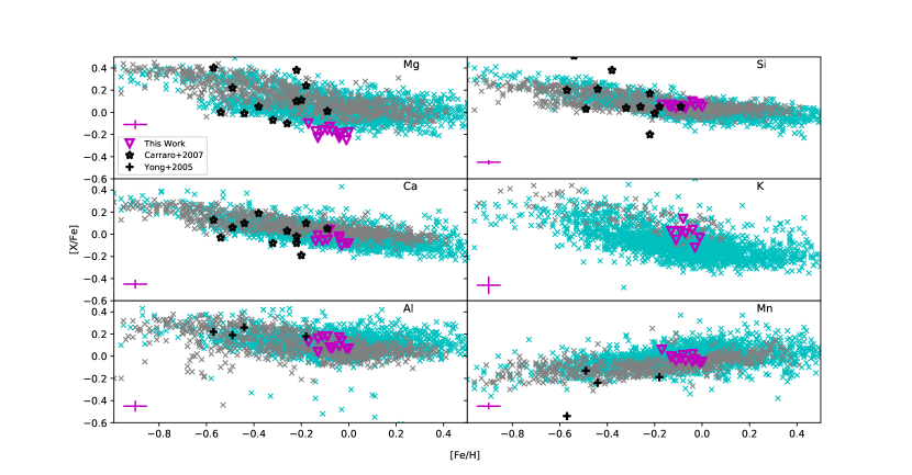
Figure 6: IC 166 results are compared with the literature, cyan crosses for Hawkins et al. (2016) results, while gray crosses for Ca, Mg, Si, and Al abundances from Bensby et al. (2014). The sources of the gray crosses for K and Mn are Chen et al. (2000) and Battistini & Bensby (2015), respectively. The Galactic anti-center OCs from Carraro et al. (2007) and Yong et al. (2005) are shown as black stars and black pluses, respectively.

4.4 OC Metallicity trend around R_GC of IC 166

Studies of the Galactic radial metallicity gradient (Friel, 1995; Frinchaboy et al., 2013; Jacobson et al., 2016; Cunha et al., 2016) are critical to understand the chemical evolution of the Galactic disc. Open clusters are one of the best tracers for this purpose, because they are located along the whole Galactic disc and they provide relatively easily measured chemical and kinematic properties. Most works agree that the metallicity decreases with increasing Galactic radius, at least for older OCs. However, the exact value of the metallicity gradient slope is still unclear (Jacobson et al., 2016; Cunha et al., 2016), nor the location of a possible break in the metallicity trend (Yong et al., 2012; Reddy et al., 2016).

In this work, we analyze the high-resolution spectra of IC 166 stars, and derive a metallicity of [Fe/H$]=-0.08\pm 0.05$ dex. Since IC 166 (R${}_{GC}\approx$12.7 kpc) is located near the possible transition zone around R${}_{GC}\approx 10-13$ kpc (Frinchaboy et al., 2013; Yong et al., 2012; Reddy et al., 2016), it may be enlightening to compare our results to the other high-resolution chemical abundance analysis on OCs near this region. For example, at R${}_{GC}\approx$10.5 kpc, Sales Silva et al. (2016) derived a metallicity of $-0.02\pm 0.05$ dex for Tombaugh 1; Souto et al. (2016) reported a metallicity of $-0.16\pm 0.04$ dex for NGC 2420 at R${}_{GC}\approx$11 kpc. More strikingly, Reddy et al. (2016) showed that the metallicities of OCs between $10-13$ kpc (including about 15 OCs) vary between 0 and $-0.4$ (their Figure 4). They suggested this region is the transition zone between thin disc OCs and thick disc OCs. Therefore, IC 166, Tombaugh 1, and NGC 2420 safely fit in the metallicity range defined by other OCs in this region. A discussion about the existence of this break requires a large number of OCs at different R_GC, which is certainly beyond the scope of this single OC concentrated work. Readers are referred to Yong et al. (2012); Reddy et al. (2016) for discussion about this topic.

4.5 [$\alpha$/Fe] versus [Fe/H]

As noted above, $\alpha$-elements are formed from reactions with $\alpha$-particles (He nuclei), which are active in Type II SNe. On the other hand, Fe is generated in SN Ia (although also, in smaller amounts, in SNe II); therefore [$\alpha$/Fe] is related to the ratio of Type II over Type Ia SNe that have enriched a particular star-forming environment.

Because the main polluters of the ISM in the early stages of galaxy formation are Type II SNe, we see enhanced $\alpha$-element abundances at low metallicities. After $\sim 1$ Gyr, Type Ia SNe start to explode, generating a significant amount of iron-peak elements but insignificant amounts of $\alpha$-elements, and the iron-peak element fraction in the ISM increases quickly (Bensby et al., 2005); [$\alpha$/Fe] decreases as the metallicity increases.

Figure 7 shows stars from APOGEE DR14 as gray dots. Results from ASPCAP DR13 for five OCs (M67, NGC 7789, NGC 6819, NGC 6791, NGC 188 in green, red, yellow, blue and pink dots, respectively) studied by Linden et al. (2017) are added, and also the results from this study for IC 166 (purple dots). The $\alpha$-elements in this plot are an average of the elements Mg, Si and Ca. All of the IC 166 stars are close to the expected trend for thin disc stars (with a mean [$\alpha$/Fe]$\sim$-0.05), although our abundance results are slightly more scattered when compared to the results for the other clusters.

IC 166 falls within the region of low $\alpha$-sequence. Thus the chemical signatures of IC 166, appear to follow the same abundance trends as thin disc field stars (see Figure 7); very similar to other know disc OCs like NGC 7062, IC1369, FSR 942, FSR 821 and FSR 941 studied in Frinchaboy et al. (2013).

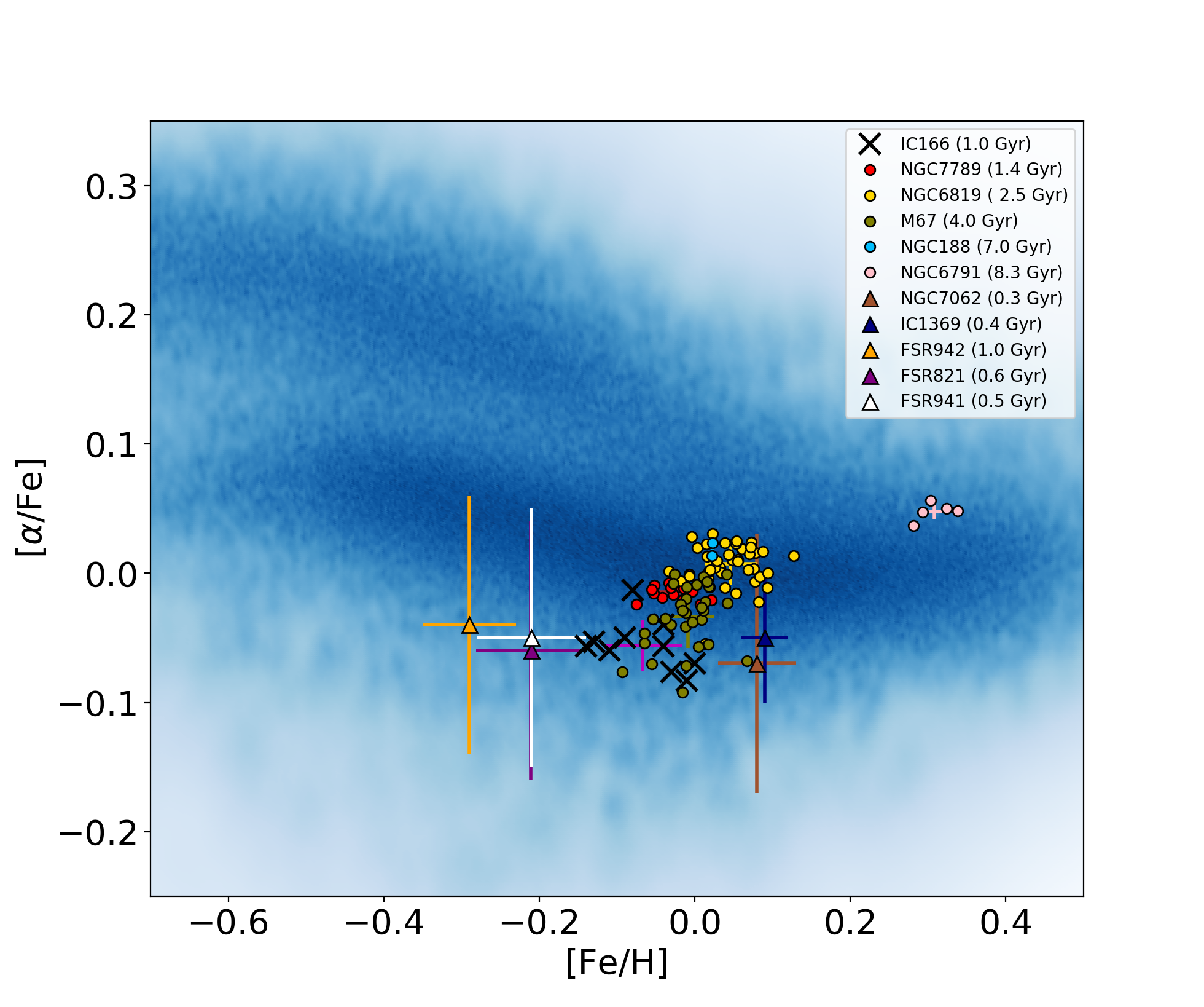
Figure 7: Density map for [$\alpha$/Fe] versus [Fe/H], illustrating the high and low $\alpha$-sequence formed by thick and thin disc stars observed by APOGEE DR14. Five open clusters studied by Linden et al. (2017) (M67, NGC 7789, NGC 6819, NGC6791, NGC 188 in green, red, yellow, pink, and cyan dots, respectively) are also shown. A sample of five new OCs (NGC 7062, IC1369, FSR 942, FSR 821, FSR 941 in brown, blue, orange, purlple and white triangles, respectively) studied by Frinchaboy et al. (2013) poorly alpha-enriched. Stars of IC 166 are shown as black ”x” symbols. The colored crosses show the mean abundances and the standard deviation for each cluster.

5 The orbit of IC 166

In order to estimate for the first time a probable Galactic orbit for IC 166, the positional information of IC 166, $(\alpha_{J2000},\delta_{J2000})=01^{h}46^{m},61^{\circ}23^{\prime}$, was combined with the newly-measured proper motions and parallaxes from Gaia DR2 (Gaia Collaboration et al., 2018; Lindegren et al., 2018) as well as with the existing line-of-sight velocities from the APOGEE survey. There were 13 stars in our sample, which were in the Gaia DR2 catalogue and had a good parallax signal-to-noise ($\pi/\pi_{\omega}>3$; see Table 3). For the 13 members surveyed by APOGEE (for which the membership is most certain) we estimate the mean proper motion of IC 166 as ($\mu_{\alpha},\mu_{\delta}$) $=$ (-1.429$\pm$0.083 , 1.139$\pm$0.075) mas yr^-1, a radial velocity of -40.58$\pm$1.59 km s^-1, and a median parallax, ($\langle\pi\rangle\pm\sigma_{\pi}$)$=(0.18466\pm 0.05095)$ , distance of 5.415$\pm$1.494 kpc, our distance estimated from parallax tend to agree with the mean distance estimated from a Bayesian approach using priors based on an assumed density distribution of the Milky Way (e.g., Bailer-Jones et al., 2018), 4.485$\pm$0.89 kpc. It is important to note that our assumed Monte Carlo approach to compute the orbital elements are similars adopting both distance estimates, and therefore do not affect the results presented in this work.

For the Galactic model we employ the Galactic dynamic software GravPot16 (Fernández-Trincado et al. 2018, in preparation), a semi-analytic, steady-state, three dimensional gravitational potential based on the mass density distributions of the Besançon Galactic model (Robin et al., 2003, 2012, 2014), observationally and dynamically constrained. The model is constituted by seven thin disc components, two thick discs, an interstellar medium (ISM), a Hernquist stellar halo, a rotating bar component, and is surrounded by a spherical dark matter halo component that fits fairly well the structural and dynamical parameters of the Milky Way to the best we know them. A description of this model and its updated parameters appears in a score of papers (Fernández-Trincado et al., 2016; Fernández-Trincado et al., 2017a, b, c; Tang et al., 2017, 2018; Libralato et al., 2018).

The Galactic potential is scaled to the Sun’s galactocentric distance, 8.3$\pm$0.23 kpc, and the local rotation velocity, 239$\pm$7 km s¹ (e.g., Brunthaler et al., 2011). We assumed the Sun’s orbital velocity vector [U_⊙,V_⊙,W_⊙]=[11.1${}^{+0.69}_{-0.75}$, 12.24${}^{+0.47}_{-0.47}$, 7.25${}^{+0.37}_{-0.36}$] (Schönrich et al., 2010). A long list of studies in the literature has presented different ranges for the bar pattern speeds. For our computations, the values $\Omega_{bar}=$ 35, 40, 45, and 50 km s^-1 kpc^-1 are employed. These values are consistent with the recent estimate of $\Omega_{bar}$ given by Portail et al. (2017); Monari et al. (2017a, b); Fernández-Trincado et al. (2017b). We consider an angle of $\phi=20^{\circ}$ for the present-day orientation of the major axis of the Galactic bar and the Sun-Galactic center line. The total mass of the bar taken in this work is 1.1$\times$10¹⁰ M_⊙, which corresponds to the dynamical constraints towards the Milky Way bulge from massless particle simulations Fernández-Trincado et al. (2017b) and is consistent with the recent estimate given by Portail et al. (2017).

Table 6: Orbital elements of IC 166 estimated with the newly-measured proper motions and parallax from Gaia DR2 data combined with existing line-of-sight velocities from APOGEE. The average value of the orbital parameters of IC 166 was found for one mllion realizations adopting a Monte Carlo approach, with uncertainty ranges given by the 16th (subscript) and 84th (superscript) percentile values.

${\Omega}_{\rm bar}$	$\langle$$r_{\rm peri}$$\rangle$	$\langle$$r_{\rm apo}$$\rangle$	$\langle$$|z|_{\rm max}$$\rangle$	$\langle$$e$$\rangle$
(km s-1 kpc-1)	(kpc)	(kpc)	(kpc)
35	12.44${}^{14.09}_{10.80}$	16.51${}^{20.88}_{12.74}$	1.49${}^{2.34}_{0.68}$	0.13${}^{0.19}_{0.07}$
40	12.45${}^{14.09}_{11.01}$	16.49${}^{20.82}_{11.98}$	1.49${}^{2.34}_{0.65}$	0.13${}^{0.20}_{0.06}$
45	12.47${}^{14.08}_{11.05}$	16.45${}^{20.87}_{11.85}$	1.49${}^{2.34}_{0.64}$	0.12${}^{0.20}_{0.05}$
50	12.48${}^{14.09}_{11.01}$	16.42${}^{20.88}_{11.95}$	1.49${}^{2.34}_{0.65}$	0.12${}^{0.20}_{0.05}$

The probable orbit of IC 166 is computed adopting a simple Monte Carlo procedure for different bar pattern speeds as mentioned above. For each of 10³ simulations, we time-integrated backwards the orbits for 2.5 Gyr under variations of the initial conditions (proper motions, radial velocity, heliocentric distance, Solar position, Solar motion and the velocity of the local standard of rest) according to their estimated errors, where the errors are assumed to follow a Gaussian distribution. The results of these computations are showed in Figure 8. The same figures display the probability densities of the resulting orbits projected on the meridional and equatorial Galactic planes in the non-inertial reference frame where the bar is at rest. The yellow and red colors correspond to more probable regions of the space, which are crossed more frequently by the simulated orbits. The final point of each of these orbits has a very similar position to the current one of IC 166.

The median values of the orbital elements for the 10³ realizations are listed in Table 6. Uncertainties in the orbital integrations are estimated as the 16th (lower limit) and 84th (upper limit) percentile values. We defined the orbital eccentricity as:

$$e=\frac{(r_{apo}-r_{peri})}{(r_{apo}+r_{peri})},$$

where $r_{apo}$ is the apogalactic distance and $r_{peri}$ the perigalactic distance. We find the orbit of IC 166 lies in the Galactic disc and it appears to be an unremarkable typical Galactic open cluster.

6 Conclusions

We have presented the first high resolution spectroscopic observations of the stellar cluster IC 166, which was recently surveyed in the H-band of APOGEE. Based on their sky distribution, radial velocity, metallicity, CMD position and proper motions, we have identified 13 highest likelihood cluster members. We derived for the first time manual abundance determinations for up to 8 chemical species (Mg, Ca, Ti, Si, Al, K, Fe, Mn). High-resolution spectra are consistent with the cluster having a metallicity of [Fe/H]$=$ -0.08$\pm$0.05 dex. Isochrone fits indicate that the cluster is about 1.0$\pm$0.2 Gyr in age.

The results presented here show the cluster lies in the low-$\alpha$ sequence near the solar neighborhood, i.e., the cluster lies in the locus dominated by the low-$\alpha$ sequence of the canonical thin disc. We also found excellent agreement between our chemical abundances and general Galactic trends from large scale studies.

It is important to note that our manual analysis was able to reduce the dispersion found by APOGEE/ASPCAP pipeline for most of the chemical species studied in this work. The most notable improvement was for [Al/Fe] abundance ratios.

Lastly, numerical integration of the possible orbits of IC 166 shows that the cluster appears to be an unremarkable standard Galactic open cluster with an orbit bound to the Galactic plane. The maximum and minimum Galactic distance achieved by the cluster as well as its orbital eccentricity suggest star formation at large Galactocentric radii. These results suggest that IC 166 could have formed nearer the solar neighborhood, fully compatible with the majority of known Galactic open clusters at similar metallicity. However, the derived orbital eccentricity ($\sim 0.13$) of the cluster is found be compatible with thin disc populations, but the maximum height above the plane, Zmax, larger than 1.5 kpc like IC 166 is too high for the thin disc and more compatible with the thick disc. It is important to note that, because the orbital excursions in our simulations are in the external part of the Galaxy (up to 16.5 kpc), it is in a region where the disc of the Milky Way is know to exhibit a significant flare (e.g., Reylé et al., 2009) and warp (Momany et al., 2006; Carraro et al., 2007). Such dynamical behaviour have been also observed in anti-center old open clusters, like Gaia 1 (e.g., Koposov et al., 2017; Koch et al., 2018; Carraro, 2018).

We further note some important limitations of our orbital calculations: we ingore secular changes in the Milky Way potential over time. We also ignore the fact that the Milky Way disc exibit a prominent warp and flare in the direction of IC 166. The Milky Way potential that we used in the simulations is made-up of the seven time independent thin discs (Robin et al., 2003) with Einasto laws (Einasto, 1979).

Appendix A Elemental abundances line-by-line

Table A1: Atomic Lines used and Derived Abundances.

Element	$\lambda_{air}$	star1	star2	star3	star4	star5	star6	star7	star8	star9	star10	star11	star12	star13
Fe	15194.50	7.34	7.46	7.31	7.32	7.50	7.56	…	7.43	7.35	…	…	7.39	7.40
	15207.50	7.36	7.55	7.22	7.36	7.40	7.52	7.40	7.36	7.33	7.46	7.23	7.37	7.29
	15490.30	7.45	7.40	7.49	7.53	7.54	7.47	7.40	…	7.32	…	7.43	7.50	…
	15648.50	7.36	7.42	…	…	7.34	7.45	7.37	7.18	7.34	…	…	7.33	7.28
	15964.90	7.28	7.58	7.41	7.37	7.40	7.46	7.34	…	7.29	7.48	7.15	7.42	7.25
	16040.70	7.29	…	…	7.54	7.42	7.28	7.49	7.32	7.36	7.47	7.31	7.29	7.37
	16153.20	7.28	7.41	7.27	7.35	7.38	7.40	7.36	…	7.21	7.48	7.26	7.32	7.25
	16165.00	7.33	7.29	7.46	…	7.33	7.26	7.32	…	7.36	7.34	…	7.36	…
	$\langle$A(Fe)$\rangle$	7.34$\pm$0.06	7.44$\pm$0.10	7.36$\pm$0.11	7.41$\pm$ 0.10	7.41$\pm$0.07	7.42$\pm$0.11	7.38$\pm$0.05	7.32$\pm$0.10	7.32$\pm$0.05	7.45$\pm$0.06	7.28$\pm$0.10	7.37$\pm$0.06	7.31$\pm$0.06
	[Fe/H]	-0.11$\pm$0.06	-0.01$\pm$0.10	-0.09$\pm$0.11	-0.04$\pm$0.10	-0.04$\pm$0.07	-0.03$\pm$0.11	-0.07$\pm$0.05	-0.13$\pm$0.10	-0.13$\pm$0.05	0.00$\pm$0.06	-0.17$\pm$0.10	-0.08$\pm$0.06	-0.14$\pm$0.06
Mg	15740.70	7.27	7.27	7.31	7.30	7.33	7.28	7.37	7.20	7.23	7.38	7.19	7.36	7.19
	15748.90	7.25	7.30	7.28	7.25	7.29	7.30	7.28	7.15	7.14	7.36	7.34	7.28	7.26
	15765.80	7.26	7.23	7.26	7.23	7.29	7.34	7.23	7.15	7.17	7.31	…	7.10	7.20
	$\langle$A(Mg)$\rangle$	7.26$\pm$0.01	7.27$\pm$0.03	7.28$\pm$0.02	7.26$\pm$0.04	7.30$\pm$0.02	7.31$\pm$0.03	7.29$\pm$0.07	7.17$\pm$0.03	7.18$\pm$0.04	7.35$\pm$0.04	7.26$\pm$0.11	7.32$\pm$0.06	7.22$\pm$0.04
	[Mg/Fe]	-0.16$\pm$0.01	-0.25$\pm$0.03	-0.16$\pm$0.02	-0.23$\pm$0.04	-0.19$\pm$0.02	-0.19$\pm$0.03	-0.17$\pm$0.07	-0.23$\pm$0.03	-0.22$\pm$0.04	-0.18$\pm$0.04	-0.10$\pm$0.11	-0.13$\pm$0.06	-0.17$\pm$0.04
Ca	16136.80	…	6.07	6.04	6.17	6.14	6.09	…	…	…	…	…	…	…
	16150.80	6.05	6.29	6.30	6.17	6.26	6.28	…	…	6.04	6.28	…	6.18	6.11
	16157.40	6.13	…	…	6.25	6.29	…	…	…	6.30	6.18	…	…	…
	16197.10	6.25	6.29	…	6.34	6.31	…	…	…	…	…	…	6.36	…
	$\langle$A(Ca)$\rangle$	6.14$\pm$0.10	6.22$\pm$0.13	6.17$\pm$0.18	6.23$\pm$0.08	6.25$\pm$0.08	6.18$\pm$0.13	…	…	6.17$\pm$0.18	6.23$\pm$0.07	…	6.27$\pm$0.13	6.11
	[Ca/Fe]	-0.06$\pm$0.10	-0.08$\pm$0.13	-0.05$\pm$0.18	-0.04$\pm$0.08	-0.02$\pm$0.08	-0.10$\pm$0.13	…	…	-0.01$\pm$0.18	-0.08$\pm$0.07	…	0.04$\pm$0.13	-0.06
K	15163.10	4.85	5.01	5.08	…	5.12	…	5.02	…	…	…	…	…	…
	15168.40	4.99	5.08	4.97	…	5.15	4.93	…	4.98	…	…	…	5.14	…
	$\langle$A(K)$\rangle$	4.92$\pm$0.10	5.04$\pm$0.05	5.02$\pm$0.08	…	5.13$\pm$0.02	4.93	5.02	4.98	…	…	…	5.14	…
	[K/Fe]	-0.05$\pm$0.10	-0.03$\pm$0.05	0.03$\pm$0.08	…	0.04$\pm$0.02	-0.12	0.01	0.03	…	…	…	0.14	…
Si	15376.80	7.32	7.46	…	…	7.45	7.59	…	7.40	…	…	…	7.46	…
	15557.80	7.42	7.63	7.39	7.58	7.54	7.59	7.39	7.42	…	7.55	…	7.27	7.36
	15884.50	7.29	7.45	…	7.32	7.44	7.40	7.33	7.29	7.33	7.38	7.21	7.31	7.19
	15960.10	7.64	7.73	7.55	7.54	7.73	7.59	7.59	…	7.55	7.59	7.38	7.88	7.55
	16060.00	…	…	…	7.79	…	…	…	7.45	…	…	7.66	7.53	7.52
	16094.80	…	7.58	7.53	…	7.52	7.43	7.43	…	7.50	7.54	…	7.61	7.45
	16215.70	…	7.71	…	7.55	7.64	7.73	…	…	7.49	7.74	7.55	…	…
	16241.80	…	7.71	…	7.64	…	…	7.56	7.49	7.56	…	7.51	7.36	…
	16680.80	7.51	7.38	7.45	…	7.61	7.45	7.51	7.41	7.39	7.57	7.42	7.42	7.51
	16828.20	…	…	…	…	…	…	…	7.55	7.37	…	…	…	…
	$\langle$A(Si)$\rangle$	7.44$\pm$0.14	7.58$\pm$0.14	7.48$\pm$0.07	7.57$\pm$0.15	7.56$\pm$0.10	7.54$\pm$0.12	7.48$\pm$0.10	7.43$\pm$0.08	7.45$\pm$0.09	7.56$\pm$0.11	7.41$\pm$0.13	7.48$\pm$0.20	7.43$\pm$0.13
	[Si/Fe]	0.04$\pm$0.14	0.08$\pm$0.14	0.06$\pm$0.07	0.10$\pm$0.15	0.09$\pm$0.10	0.06$\pm$0.12	0.04$\pm$0.10	0.05$\pm$0.08	0.07$\pm$0.09	0.05$\pm$0.11	0.07$\pm$0.13	0.05$\pm$0.20	0.06$\pm$0.13
Ti	15715.60	4.71	4.78	…	…	…	…	…	…	…	4.84	…	…	4.78
	$\langle$A(Ti)$\rangle$	4.71	4.78	…	…	…	…	…	…	…	4.84	…	…	4.78
	[Ti/Fe]	-0.08	-0.11	…	…	…	…	…	…	…	-0.06	…	…	0.02
Mn	15159.20	5.26	5.28	…	5.28	…	5.34	…	5.26	…	5.34	…	5.31	…
	15217.70	5.23	5.38	5.37	5.25	5.37	5.32	5.31	5.23	5.19	5.34	5.27	…	…
	15262.40	…	5.29	5.20	5.37	…	…	5.25	5.29	5.32	5.35	5.30	5.33	…
	$\langle$A(Mn)$\rangle$	5.24$\pm$0.02	5.32$\pm$0.05	5.28$\pm$0.12	5.30$\pm$0.06	5.37	5.33$\pm$0.01	5.28$\pm$0.04	5.26$\pm$0.03	5.25$\pm$0.09	5.34$\pm$0.01	5.28$\pm$0.02	5.32$\pm$0.01	…
	[Mn/Fe]	-0.04$\pm$0.02	-0.06$\pm$0.05	-0.02$\pm$0.12	-0.05$\pm$0.06	0.02	-0.03$\pm$0.01	-0.04$\pm$0.04	0.00$\pm$0.03	-0.01$\pm$0.09	-0.05$\pm$0.01	0.06$\pm$0.02	0.01$\pm$0.01	…
Al	16719.00	6.51	6.45	6.47	6.47	…	…	6.43	6.38	6.45	6.51	…	6.39	…
	16750.60	6.37	6.41	6.45	6.37	6.50	6.48	6.32	6.18	6.36	6.39	6.33	6.37	…
	$\langle$A(Al)$\rangle$	6.44$\pm$0.10	6.43$\pm$0.03	6.46$\pm$0.01	6.42$\pm$0.07	6.50	6.48	6.37$\pm$0.08	6.28$\pm$0.14	6.40$\pm$0.06	6.45$\pm$0.08	6.33	6.38$\pm$0.01	…
	[Al/Fe]	0.18$\pm$0.10	0.07$\pm$0.03	0.18$\pm$0.01	0.09$\pm$0.07	0.17	0.14	0.07$\pm$0.08	0.04$\pm$0.14	0.16$\pm$0.06	0.07$\pm$0.08	0.13	0.08$\pm$0.01	…

Appendix B Orbit of IC 166 with Monte Carlo calculations

Figure 8 shows the Monte Carlo simulations for the bound orbit of IC 166, we make these Monte Carlo simulations to estimate the uncertainties in the orbital elements (see text).

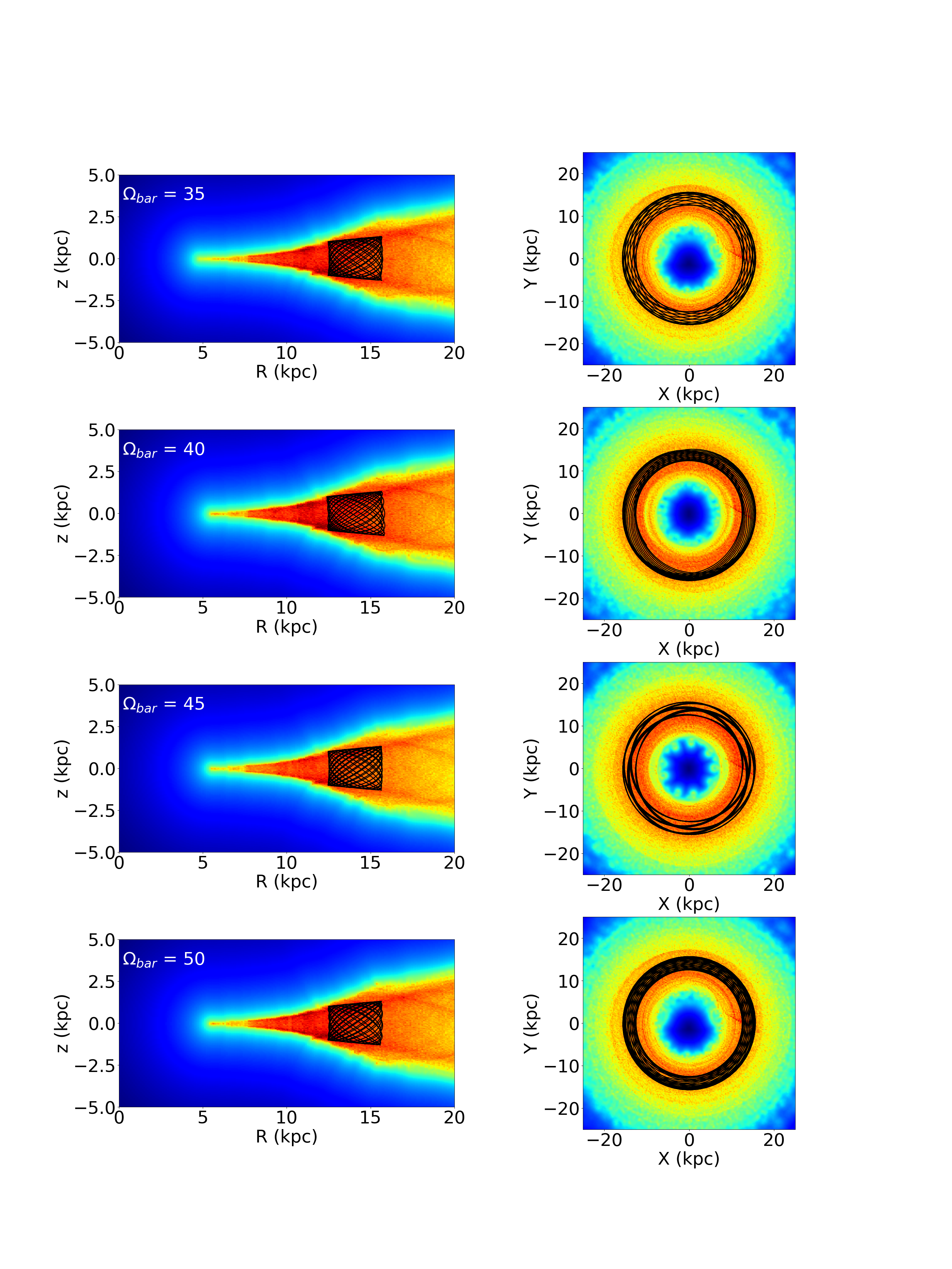
Figure 8: Probability density maps color-coded at the bottom for the meridional orbits in the $R,z$ plane (column 1) and face-on (column 2) of a thousand random realizations of IC 166 time-integrated backwards for 2.5 Gyr adopting the newly-measured proper motions and parallax from Gaia DR2 (Gaia Collaboration et al., 2018; Lindegren et al., 2018) . Red and yellow colors correspond to larger probabilities. The tile size of the HealPix map is 0.10 kpc². The black line shows the orbit using the best values found for the cluster (see text).

References

- Abolfathi et al. (2018) Abolfathi, B., Aguado, D. S., Aguilar, G., et al. 2018, ApJS, 235, 42
- Allende Prieto et al. (2006) Allende Prieto, C., Beers, T. C., Wilhelm, R., et al. 2006, ApJ, 636, 804
- Arnould et al. (1999) Arnould, M., Goriely, S., & Jorissen, A. 1999, A&A, 347, 572
- Asplund et al. (2005) Asplund, M., Grevesse, N., & Sauval, A. J. 2005, in Astronomical Society of the Pacific Conference Series, Vol. 336, Cosmic Abundances as Records of Stellar Evolution and Nucleosynthesis, ed. T. G. Barnes, III & F. N. Bash, 25
- Bailer-Jones et al. (2018) Bailer-Jones, C. A. L., Rybizki, J., Fouesneau, M., Mantelet, G., & Andrae, R. 2018, ArXiv e-prints, arXiv:1804.10121
- Battistini & Bensby (2015) Battistini, C., & Bensby, T. 2015, A&A, 577, A9
- Bensby et al. (2005) Bensby, T., Feltzing, S., Lundström, I., & Ilyin, I. 2005, A&A, 433, 185
- Bensby et al. (2014) Bensby, T., Feltzing, S., & Oey, M. S. 2014, A&A, 562, A71
- Blanton et al. (2017) Blanton, M. R., Bershady, M. A., Abolfathi, B., et al. 2017, AJ, 154, 28
- Bonatto et al. (2006) Bonatto, C., Kerber, L. O., Bica, E., & Santiago, B. X. 2006, A&A, 446, 121
- Bressan et al. (2012) Bressan, A., Marigo, P., Girardi, L., et al. 2012, MNRAS, 427, 127
- Brunthaler et al. (2011) Brunthaler, A., Reid, M. J., Menten, K. M., et al. 2011, Astronomische Nachrichten, 332, 461
- Burkhead (1969) Burkhead, M. S. 1969, AJ, 74, 1171
- Carraro (2018) Carraro, G. 2018, Research Notes of the American Astronomical Society, 2, 12
- Carraro & Chiosi (1994) Carraro, G., & Chiosi, C. 1994, A&A, 287, 761
- Carraro et al. (2007) Carraro, G., Geisler, D., Villanova, S., Frinchaboy, P. M., & Majewski, S. R. 2007, A&A, 476, 217
- Carraro et al. (1998) Carraro, G., Ng, Y. K., & Portinari, L. 1998, MNRAS, 296, 1045
- Chen et al. (2000) Chen, Y. Q., Nissen, P. E., Zhao, G., Zhang, H. W., & Benoni, T. 2000, A&AS, 141, 491
- Clayton (2007) Clayton, D. 2007, Handbook of Isotopes in the Cosmos
- Cunha et al. (2016) Cunha, K., Frinchaboy, P. M., Souto, D., et al. 2016, Astronomische Nachrichten, 337, 922
- Cunha et al. (2017) Cunha, K., Smith, V. V., Hasselquist, S., et al. 2017, ApJ, 844, 145
- de la Fuente Marcos & de la Fuente Marcos (2004) de la Fuente Marcos, R., & de la Fuente Marcos, C. 2004, New A, 9, 475
- De Silva et al. (2015) De Silva, G. M., Freeman, K. C., Bland-Hawthorn, J., et al. 2015, MNRAS, 449, 2604
- Deng & Xin (2007) Deng, L., & Xin, Y. 2007, in Astronomical Society of the Pacific Conference Series, Vol. 374, From Stars to Galaxies: Building the Pieces to Build Up the Universe, ed. A. Vallenari, R. Tantalo, L. Portinari, & A. Moretti, 387
- Dias et al. (2002) Dias, W. S., Alessi, B. S., Moitinho, A., & Lépine, J. R. D. 2002, A&A, 389, 871
- Dias et al. (2014) Dias, W. S., Monteiro, H., Caetano, T. C., et al. 2014, A&A, 564, A79
- Donati et al. (2014) Donati, P., Cantat Gaudin, T., Bragaglia, A., et al. 2014, A&A, 561, A94
- Einasto (1979) Einasto, J. 1979, in IAU Symposium, Vol. 84, The Large-Scale Characteristics of the Galaxy, ed. W. B. Burton, 451–458
- Fernández-Trincado et al. (2017a) Fernández-Trincado, J. G., Geisler, D., Moreno, E., et al. 2017a, in SF2A-2017: Proceedings of the Annual meeting of the French Society of Astronomy and Astrophysics, ed. C. Reylé, P. Di Matteo, F. Herpin, E. Lagadec, A. Lançon, Z. Meliani, & F. Royer, 199–202
- Fernández-Trincado et al. (2017b) Fernández-Trincado, J. G., Robin, A. C., Moreno, E., Pérez-Villegas, A., & Pichardo, B. 2017b, in SF2A-2017: Proceedings of the Annual meeting of the French Society of Astronomy and Astrophysics, ed. C. Reylé, P. Di Matteo, F. Herpin, E. Lagadec, A. Lançon, Z. Meliani, & F. Royer, 193–198
- Fernández-Trincado et al. (2016) Fernández-Trincado, J. G., Robin, A. C., Moreno, E., et al. 2016, ApJ, 833, 132
- Fernández-Trincado et al. (2017c) Fernández-Trincado, J. G., Zamora, O., García-Hernández, D. A., et al. 2017c, ApJ, 846, L2
- Fernández-Trincado et al. (2018) Fernández-Trincado, J. G., Zamora, O., Souto, D., et al. 2018, ArXiv e-prints, arXiv:1801.07136
- Friel (1995) Friel, E. D. 1995, ARA&A, 33, 381
- Friel (2013) —. 2013, Open Clusters and Their Role in the Galaxy, ed. T. D. Oswalt & G. Gilmore, 347
- Friel & Janes (1993) Friel, E. D., & Janes, K. A. 1993, A&A, 267, 75
- Friel et al. (1989) Friel, E. D., Liu, T., & Janes, K. A. 1989, PASP, 101, 1105
- Friel et al. (2014) Friel, E. D., Donati, P., Bragaglia, A., et al. 2014, A&A, 563, A117
- Frinchaboy et al. (2013) Frinchaboy, P. M., Thompson, B., Jackson, K. M., et al. 2013, ApJ, 777, L1
- Gaia Collaboration et al. (2018) Gaia Collaboration, Brown, A. G. A., Vallenari, A., et al. 2018, ArXiv e-prints, arXiv:1804.09365
- García Pérez et al. (2016) García Pérez, A. E., Allende Prieto, C., Holtzman, J. A., et al. 2016, AJ, 151, 144
- Geisler et al. (1997) Geisler, D., Claria, J. J., & Minniti, D. 1997, PASP, 109, 799
- Gieles et al. (2006) Gieles, M., Portegies Zwart, S. F., Baumgardt, H., et al. 2006, MNRAS, 371, 793
- Gieles & Renaud (2016) Gieles, M., & Renaud, F. 2016, MNRAS, 463, L103
- Gilmore et al. (2012) Gilmore, G., Randich, S., Asplund, M., et al. 2012, The Messenger, 147, 25
- Gunn et al. (2006) Gunn, J. E., Siegmund, W. A., Mannery, E. J., et al. 2006, AJ, 131, 2332
- Gustafsson et al. (2008) Gustafsson, B., Edvardsson, B., Eriksson, K., et al. 2008, A&A, 486, 951
- Hasselquist et al. (2016) Hasselquist, S., Shetrone, M., Cunha, K., et al. 2016, ApJ, 833, 81
- Hawkins et al. (2016) Hawkins, K., Masseron, T., Jofré, P., et al. 2016, A&A, 594, A43
- Hayden et al. (2015) Hayden, M. R., Bovy, J., Holtzman, J. A., et al. 2015, ApJ, 808, 132
- Jacobson et al. (2016) Jacobson, H. R., Friel, E. D., Jílková, L., et al. 2016, A&A, 591, A37
- Janes (1979) Janes, K. A. 1979, ApJS, 39, 135
- Kharchenko et al. (2012) Kharchenko, N. V., Piskunov, A. E., Schilbach, E., Röser, S., & Scholz, R.-D. 2012, A&A, 543, A156
- Koch et al. (2018) Koch, A., Hansen, T. T., & Kunder, A. 2018, A&A, 609, A13
- Koposov et al. (2017) Koposov, S. E., Belokurov, V., & Torrealba, G. 2017, MNRAS, 470, 2702
- Lamers & Gieles (2006) Lamers, H. J. G. L. M., & Gieles, M. 2006, A&A, 455, L17
- Lamers et al. (2005) Lamers, H. J. G. L. M., Gieles, M., Bastian, N., et al. 2005, A&A, 441, 117
- Libralato et al. (2018) Libralato, M., Bellini, A., Bedin, L. R., et al. 2018, ApJ, 854, 45
- Lindegren et al. (2018) Lindegren, L., Hernandez, J., Bombrun, A., et al. 2018, ArXiv e-prints, arXiv:1804.09366
- Linden et al. (2017) Linden, S. T., Pryal, M., Hayes, C. R., et al. 2017, ApJ, 842, 49
- Liu et al. (2016) Liu, F., Yong, D., Asplund, M., Ramírez, I., & Meléndez, J. 2016, MNRAS, 457, 3934
- Loktin & Beshenov (2003) Loktin, A. V., & Beshenov, G. V. 2003, Astronomy Reports, 47, 6
- Magrini et al. (2009) Magrini, L., Sestito, P., Randich, S., & Galli, D. 2009, A&A, 494, 95
- Magrini et al. (2015) Magrini, L., Randich, S., Donati, P., et al. 2015, A&A, 580, A85
- Majewski et al. (2017) Majewski, S. R., Schiavon, R. P., Frinchaboy, P. M., et al. 2017, AJ, 154, 94
- Masseron et al. (2016) Masseron, T., Merle, T., & Hawkins, K. 2016, BACCHUS: Brussels Automatic Code for Characterizing High accUracy Spectra, Astrophysics Source Code Library, ascl:1605.004
- Momany et al. (2006) Momany, Y., Zaggia, S., Gilmore, G., et al. 2006, A&A, 451, 515
- Monari et al. (2017a) Monari, G., Famaey, B., Siebert, A., et al. 2017a, MNRAS, 465, 1443
- Monari et al. (2017b) Monari, G., Kawata, D., Hunt, J. A. S., & Famaey, B. 2017b, MNRAS, 466, L113
- Moyano Loyola & Hurley (2013) Moyano Loyola, G. R. I., & Hurley, J. R. 2013, MNRAS, 434, 2509
- Portail et al. (2017) Portail, M., Gerhard, O., Wegg, C., & Ness, M. 2017, MNRAS, 465, 1621
- Randich et al. (2013) Randich, S., Gilmore, G., & Gaia-ESO Consortium. 2013, The Messenger, 154, 47
- Reddy et al. (2016) Reddy, A. B. S., Lambert, D. L., & Giridhar, S. 2016, MNRAS, 463, 4366
- Reylé et al. (2009) Reylé, C., Marshall, D. J., Robin, A. C., & Schultheis, M. 2009, A&A, 495, 819
- Robin et al. (2012) Robin, A. C., Marshall, D. J., Schultheis, M., & Reylé, C. 2012, A&A, 538, A106
- Robin et al. (2003) Robin, A. C., Reylé, C., Derrière, S., & Picaud, S. 2003, A&A, 409, 523
- Robin et al. (2014) Robin, A. C., Reylé, C., Fliri, J., et al. 2014, A&A, 569, A13
- Salaris et al. (2004) Salaris, M., Weiss, A., & Percival, S. M. 2004, A&A, 414, 163
- Sales Silva et al. (2016) Sales Silva, J. V., Carraro, G., Anthony-Twarog, B. J., et al. 2016, AJ, 151, 6
- Samland (1998) Samland, M. 1998, ApJ, 496, 155
- Schönrich et al. (2010) Schönrich, R., Binney, J., & Dehnen, W. 2010, MNRAS, 403, 1829
- Souto et al. (2016) Souto, D., Cunha, K., Smith, V., et al. 2016, ApJ, 830, 35
- Subramaniam & Bhatt (2007) Subramaniam, A., & Bhatt, B. C. 2007, MNRAS, 377, 829
- Tang et al. (2018) Tang, B., Fernández-Trincado, J. G., Geisler, D., et al. 2018, ApJ, 855, 38
- Tang et al. (2017) Tang, B., Geisler, D., Friel, E., et al. 2017, A&A, 601, A56
- Twarog et al. (1997) Twarog, B. A., Ashman, K. M., & Anthony-Twarog, B. J. 1997, AJ, 114, 2556
- Vallenari et al. (2000) Vallenari, A., Carraro, G., & Richichi, A. 2000, A&A, 353, 147
- van den Bergh (2006) van den Bergh, S. 2006, AJ, 131, 1559
- Vázquez et al. (2008) Vázquez, R. A., May, J., Carraro, G., et al. 2008, ApJ, 672, 930
- Wilson et al. (2012) Wilson, J. C., Hearty, F., Skrutskie, M. F., et al. 2012, in Proc. SPIE, Vol. 8446, Ground-based and Airborne Instrumentation for Astronomy IV, 84460H
- Woosley & Weaver (1995) Woosley, S. E., & Weaver, T. A. 1995, ApJS, 101, 181
- Yong et al. (2012) Yong, D., Carney, B. W., & Friel, E. D. 2012, AJ, 144, 95
- Yong et al. (2005) Yong, D., Carney, B. W., & Teixera de Almeida, M. L. 2005, AJ, 130, 597
- Zamora et al. (2015) Zamora, O., García-Hernández, D. A., Allende Prieto, C., et al. 2015, AJ, 149, 181
- Zasowski et al. (2013) Zasowski, G., Johnson, J. A., Frinchaboy, P. M., et al. 2013, AJ, 146, 81
- Zasowski et al. (2017) Zasowski, G., Cohen, R. E., Chojnowski, S. D., et al. 2017, AJ, 154, 198
- Zhang et al. (2006) Zhang, H. W., Gehren, T., Butler, K., Shi, J. R., & Zhao, G. 2006, A&A, 457, 645