Spectator effects in the HQET renormalization group improved Lagrangian at $\mathcal{O}(1/m^{3})$ with leading logarithmic accuracy: Spin-dependent case

Abstract

The present paper incorporates the effects induced by massless spectator quarks in the renormalization group improved Wilson coefficients associated to the ${\cal O}(1/m^{3})$ spin-dependent heavy quark effective theory Lagrangian operators. The computation is carried out in Coulomb gauge with leading logarithmic precision. The result completes the Lagrangian to $\mathcal{O}(1/m^{3})$ with that accuracy.

I Introduction

The heavy quark effective theory (HQET) HQET is a powerful tool used to describe hadrons containing a heavy quark. The HQET Lagrangian is also one of the building blocks of the nonrelativistic QCD (NRQCD) Lagrangian  NRQCD ; Bodwin:1994jh , which aims to describe bound states of two heavy quarks, heavy quarkonium for short. Concurrently, the Wilson coefficients of the NRQCD Lagrangian enter into the Wilson coefficients (interaction potentials) of the potential NRQCD (pNQRCD) Lagrangian Pineda:1997bj ; Brambilla:1999xf as a consequence of the matching between the two effective theories. The later, is a theory optimised for the description of heavy quarkonium near threshold (for reviews see Refs. Brambilla:2004jw ; Pineda:2011dg ).

Therefore, the Wilson coefficients computed in this paper could have many applications in heavy quark and heavy quarkonium physics. In particular, they are necessary ingredients to obtain the pNRQCD Lagrangian with next-to-next-to-next-to-next-to-leading order (NNNNLO) and with next-to-next-to-next-to-next-to-leading logarithmic (NNNNLL) accuracy, which is the necessary precision to determine the $\mathcal{O}(m\alpha^{6})$ and the $\mathcal{O}(m\alpha^{7}\ln\alpha+m\alpha^{8}\ln^{2}\alpha+\ldots)$ heavy quarkonium spectrum. As commented in Ref. lmp , the Wilson coefficients associated to the $1/m^{3}$ spin-independent operators are also necessary to obtain the heavy quarkonium spectrum with NNNLL accuracy, and the production and annihilation of heavy quarkonium with NNLL precision inpreparation , but this is not the case for the spin-dependent ones rgsddelta . The Wilson coefficients computed in this paper also have applications in QED bound states like in muonic hydrogen. The computation presented here, also provides a cross-check that the physical combinations found in Ref. lmp are gauge independent, and also new physical quantities involving light fermion operators are found. It also provides an additional cross-check of some of the reparametrization invariance relations given in Ref. Manohar:1997qy and gives a solution in a more standard basis settled on by the same reference.

At present, the operator structure of the HQET Lagrangian, and the tree-level values of their Wilson coefficients, is known to ${\cal O}(1/m^{3})$ in the case without spectator quarks Manohar:1997qy . The inclusion of spectator quarks has been considered in Ref. Balzereit:1998am . The Wilson coefficients with leading logarithmic (LL) accuracy were computed in Refs. Finkemeier:1996uu ; Blok:1996iz ; Bauer:1997gs to ${\cal O}(1/m^{2})$ and at next-to-leading order (NLO) in Ref. Manohar:1997qy to ${\cal O}(1/m^{2})$ (without heavy-light operators). The LL running to ${\cal O}(1/m^{3})$ without the inclusion of spectator quarks was considered in Refs. Balzereit:1998jb ; Balzereit:1998vh , which turned out to have internal discrepancies between their explicit single log results and their own anomalous dimension matrix. The computation was reconsidered in Refs. chromopolarizabilities ; lmp , where the results were corrected.

The inclusion of heavy-light operators to $\mathcal{O}(1/m^{3})$ was considered in Ref. Balzereit:1998am , but only single logarithmic results for the Wilson coefficients were provided. The inclusion of spectator quarks and the obtention of the full ressumed leading logarithmic (LL) expresions for the spin-independent case were obtained in Ref. chromopolarizabilities . At the level of the single logs, these two references are in disagreement. This work is a follow-up to Refs. chromopolarizabilities ; lmp and, for this reason, is structured very similarly. The effect induced by massless spectator quarks to the running of the $\mathcal{O}(1/m^{3})$ spin-dependent operators (bilinear operators in the heavy quark fields and heavy-light operators) is included. Renormalization group improved expressions for the Wilson coefficients associated to these operators are obtained with LL accuracy. The computation is done in Coulomb gauge.

The paper is organized as follows. In Sec. II we introduce the HQET Lagrangian up to $\mathcal{O}(1/m^{3})$ including heavy-light operators (at $\mathcal{O}(1/m^{3})$ only spin-dependent heavy-light operators are included. See Ref. Balzereit:1998am for a complete basis and Ref. chromopolarizabilities for relevant spin-independent operators that get LL running). The Sec. III is dedicated to the computation of the anomalous dimensions and it is divided in three subsections: In Sec. III.1 and Sec. III.2 the renormalization group equations (RGEs) for the Wilson coefficients associated to $1/m^{3}$ heavy-light operators and to $1/m^{3}$ bilinear operators are presented, respectively. In Sec. III.3 physical combinations are sought, and their associated RGE equations are presented. The solution of the RGEs for the physical quantities, as well as its numerical analysis, is displayed in Sec. IV. We conclude in Sec. V. Finally, some necessary Feynman rules are summarized in Sec. A.

II HQET Lagrangian

The starting point is the HQET Lagrangian up to $\mathcal{O}(1/m^{3})$ for a quark of mass $m\gg\Lambda_{\rm QCD}$ in the rest frame, $v^{\mu}=(1,{\bf 0})$. It is given in Refs. Manohar:1997qy ; Balzereit:1998am , and reads:

$${\cal L}_{\rm HQET}={\cal L}_{g}+{\cal L}_{Q}+{\cal L}_{l}\,,$$ (1)

$${\cal L}_{g}=-\frac{1}{4}G^{\mu\nu\,a}G_{\mu\nu}^{a}+c_{1}^{g}\frac{g}{4m^{2}}f^{abc}G_{\mu\nu}^{a}G^{\mu\,b}{}_{\alpha}G^{\nu\alpha\,c}+{\cal O}\left(\frac{1}{m^{4}}\right),$$ (2)

$${\cal L}_{Q}=Q^{\dagger}\Biggl{\{}iD_{0}+\frac{c_{k}}{2m}{\bf D}^{2}+\frac{c_{F}}{2m}{\mbox{\boldmath$\sigma$}\cdot g{\bf B}}$$

$$+\frac{c_{D}}{8m^{2}}\left({\bf D}\cdot g{\bf E}-g{\bf E}\cdot{\bf D}\right)+i\,\frac{c_{S}}{8m^{2}}{\mbox{\boldmath$\sigma$}\cdot\left({\bf D}\times g{\bf E}-g{\bf E}\times{\bf D}\right)}$$

$$+\frac{c_{4}}{8m^{3}}{\bf D}^{4}+ic_{M}\,g{{\bf D\cdot\left[D\times B\right]+\left[D\times B\right]\cdot D}\over 8m^{3}}+c_{A_{1}}\,{g^{2}}\,{{\bf B}^{2}-{\bf E}^{2}\over 8m^{3}}-c_{A_{2}}{{g^{2}}{\bf E}^{2}\over 16m^{3}}$$

$$+c_{W_{1}}\,g{\left\{{\bf D^{2},\mbox{\boldmath$\sigma$}\cdot B}\right\}\over 8m^{3}}-c_{W_{2}}\,g{{\bf D}^{i}\,{\bf\mbox{\boldmath$\sigma$}\cdot B}\,{\bf D}^{i}\over 4m^{3}}+c_{p^{\prime}p}\,g{{\bf\mbox{\boldmath$\sigma$}\cdot D\,B\cdot D+D\cdot B\,\mbox{\boldmath$\sigma$}\cdot D}\over 8m^{3}}$$

$$+c_{A_{3}}\,{g^{2}}\,\frac{1}{N_{c}}{\rm Tr}\left({{\bf B}^{2}-{\bf E}^{2}\over 8m^{3}}\right)-c_{A_{4}}\,{g^{2}}\,\frac{1}{N_{c}}{\rm Tr}\left({{\bf E}^{2}\over 16m^{3}}\right)$$

$$+ic_{B_{1}}\,g^{2}\,{{\bf\mbox{\boldmath$\sigma$}\cdot\left(B\times B-E\times E\right)}\over 8m^{3}}-ic_{B_{2}}\,g^{2}\,{{\bf\mbox{\boldmath$\sigma$}\cdot\left(E\times E\right)}\over 8m^{3}}\Biggr{\}}Q+{\cal O}\left(\frac{1}{m^{4}}\right)\,.$$ (3)

Where $Q$ is the nonrelativistic fermion field represented by a Pauli spinor. We define $iD^{0}=i\partial^{0}-gA^{0\,a}T^{a}$ and $i{\bf D}=i\mbox{\boldmath$\nabla$}+g{\bf A}^{a}T^{a}$, where $A^{0\,a}$ and ${\bf A}^{a}$ represent the longitudinal and tranverse gluon fields, respectively. The chromoelectric field is defined as ${\bf E}^{i}=G^{i0}$, whereas the chromomagnetic field as ${\bf B}^{i}=-\epsilon^{ijk}G^{jk}/2$, where $\epsilon^{ijk}$ is the three-dimensional totally antisymmetric tensor, with $\epsilon^{123}=1$. The components of the vector $\sigma$ are the Pauli matrices. Note also the rescaling by a factor $1/N_{c}$ of the coefficients $c_{A_{3,4}}$ following Ref. chromopolarizabilities , as compared to the definitions given in Ref. Manohar:1997qy .

The inclusion of $n_{f}$ massless fermions adds an extra contribution to the HQET Lagrangian with the following structure:

$${\cal L}_{l}=\sum_{i=1}^{n_{f}}\bar{q}_{i}i\,\raise 0.6458pt\hbox{/}\mkern-13.5muDq_{i}+\frac{\delta{\cal L}^{(2)}_{q}}{m^{2}}+\frac{\delta{\cal L}^{(2)}_{Qq}}{m^{2}}+\frac{\delta{\cal L}^{(3)}_{q}}{m^{3}}+\frac{\delta{\cal L}^{(3)}_{Qq}}{m^{3}}+{\cal O}\left(\frac{1}{m^{4}}\right).$$ (4)

The complete set of operators at ${\cal O}(1/m^{2})$ can be found in Bauer:1997gs . They read

$$\delta{\cal L}^{(2)}_{Qq}=\frac{c_{1}^{hl}}{8}\,g^{2}\,\sum_{i=1}^{n_{f}}Q^{\dagger}T^{a}Q\bar{q}_{i}\gamma^{0}T^{a}q_{i}-\frac{c_{2}^{hl}}{8}\,g^{2}\,\sum_{i=1}^{n_{f}}Q^{\dagger}\mbox{\boldmath$\sigma$}^{j}T^{a}Q\bar{q}_{i}\gamma^{j}\gamma_{5}T^{a}q_{i}$$

$$\qquad\qquad+\frac{c_{3}^{hl}}{8}\,g^{2}\,\sum_{i=1}^{n_{f}}Q^{\dagger}Q\bar{q}_{i}\gamma^{0}q_{i}-\frac{c_{4}^{hl}}{8}\,g^{2}\,\sum_{i=1}^{n_{f}}Q^{\dagger}\mbox{\boldmath$\sigma$}^{j}Q\bar{q}_{i}\gamma^{j}\gamma_{5}q_{i},$$ (5)

$$\delta{\cal L}^{(2)}_{q}=\frac{c_{D}^{l}}{4}\bar{q}_{i}\gamma_{\nu}D_{\mu}G^{\mu\nu}q_{i}$$

$$\qquad\qquad+\frac{c_{1}^{ll}}{8}\,g^{2}\,\sum_{i,j=1}^{n_{f}}\bar{q_{i}}T^{a}\gamma^{\mu}q_{i}\ \bar{q}_{j}T^{a}\gamma_{\mu}q_{j}+\frac{c_{2}^{ll}}{8}\,g^{2}\,\sum_{i,j=1}^{n_{f}}\bar{q_{i}}T^{a}\gamma^{\mu}\gamma_{5}q_{i}\ \bar{q}_{j}T^{a}\gamma_{\mu}\gamma_{5}q_{j}$$

$$\qquad\qquad+\frac{c_{3}^{ll}}{8}\,g^{2}\,\sum_{i,j=1}^{n_{f}}\bar{q_{i}}\gamma^{\mu}q_{i}\ \bar{q}_{j}\gamma_{\mu}q_{j}+\frac{c_{4}^{ll}}{8}\,g^{2}\,\sum_{i,j=1}^{n_{f}}\bar{q_{i}}\gamma^{\mu}\gamma_{5}q_{i}\ \bar{q}_{j}\gamma_{\mu}\gamma_{5}q_{j}.$$ (6)

However, the light-light operators $\delta\mathcal{L}_{q}^{(2)}$ and $\delta\mathcal{L}_{q}^{(3)}$, as well as the $1/m^{2}$ gluonic operator with associated Wilson coefficient $c_{1}^{g}$, contribute at NLL or beyond, so we will not consider them any further.

The $\mathcal{O}(1/m^{3})$ (dimension 7) heavy-light operators were considered in detail in Ref. Balzereit:1998am and they can be found in Eq. (10) of that reference. However, we will not consider all of them, but only those that get LL running and that could affect the LL running of $c_{p^{\prime}p}$, $c_{W_{1}}$, $c_{W_{2}}$, $c_{B_{1}}$ and $c_{B_{2}}$. Initially, we can disregard some of them because of its spin independence or just by using the heavy quark equation of motion. After that, we face the following operators:

$$\mathcal{M}_{3\pm}^{(3h)s/o}=\pm g_{s}^{2}[\bar{q}_{l}\gamma_{\mu}\mathcal{C}_{s/o}^{a}q_{l}][\bar{h}_{v}i\sigma^{\mu\nu}\mathcal{C}_{s/o}^{a}iD_{\nu}^{\pm}h_{v}]\,,$$ (7)

$$\mathcal{M}_{5\pm}^{(3h)s/o}=\pm g_{s}^{2}[\bar{q}_{l}i\sigma_{\mu\lambda}v^{\lambda}\mathcal{C}_{s/o}^{a}q_{l}][\bar{h}_{v}i\sigma^{\mu\nu}\mathcal{C}_{s/o}^{a}iD_{\nu}^{\pm}h_{v}]\,,$$ (8)

$$\mathcal{M}_{7\pm}^{(3h)s/o}=\pm g_{s}^{2}[\bar{q}_{l}\gamma_{5}\not{v}\mathcal{C}_{s/o}^{a}q_{l}][\bar{h}_{v}\gamma_{5}\mathcal{C}_{s/o}^{a}i\not{D}^{\pm}h_{v}]\,,$$ (9)

$$\mathcal{M}_{9\pm}^{(3h)s/o}=\pm g_{s}^{2}[\bar{q}_{l}\gamma_{5}\mathcal{C}_{s/o}^{a}q_{l}][\bar{h}_{v}\gamma_{5}\mathcal{C}_{s/o}^{a}i\not{D}^{\pm}h_{v}]\,,$$ (10)

$$\mathcal{M}_{5\pm}^{(3l)s/o}=\pm g_{s}^{2}[\bar{q}_{l}i\sigma^{\mu\nu}\mathcal{C}_{s/o}^{a}(ivD^{\pm})q_{l}][\bar{h}_{v}i\sigma_{\mu\nu}\mathcal{C}_{s/o}^{a}h_{v}]\,,$$ (11)

$$\mathcal{M}_{6\pm}^{(3l)s/o}=\pm g_{s}^{2}[\bar{q}_{l}\gamma_{5}\not{v}\mathcal{C}_{s/o}^{a}iD_{\mu}^{\pm}q_{l}][\bar{h}_{v}\gamma_{5}\gamma^{\mu}\mathcal{C}_{s/o}^{a}h_{v}]\,,$$ (12)

$$\mathcal{M}_{7\pm}^{(3l)s/o}=\pm g_{s}^{2}[\bar{q}_{l}\gamma_{5}\gamma^{\mu}\mathcal{C}_{s/o}^{a}(ivD^{\pm})q_{l}][\bar{h}_{v}\gamma_{5}\gamma_{\mu}\mathcal{C}_{s/o}^{a}h_{v}]\,,$$ (13)

$$\mathcal{M}_{8\pm}^{(3l)s/o}=\pm g_{s}^{2}[\bar{q}_{l}\gamma_{5}\mathcal{C}_{s/o}^{a}iD_{\mu}^{\pm}q_{l}][\bar{h}_{v}\gamma_{5}\gamma^{\mu}\mathcal{C}_{s/o}^{a}h_{v}]\,,$$ (14)

$$\mathcal{M}_{10\pm}^{(3l)s/o}=\pm g_{s}^{2}[\bar{q}_{l}\gamma_{\nu}\mathcal{C}_{s/o}^{a}iD_{\mu}^{\pm}q_{l}][\bar{h}_{v}i\sigma^{\mu\nu}\mathcal{C}_{s/o}^{a}h_{v}]\,.$$ (15)

Where $iD_{\mu}^{+}=i\stackrel{{\scriptstyle\rightarrow}}{{\partial}}_{\mu}-gA_{\mu}^{a}T^{a}$ and $iD_{\mu}^{-}=i\stackrel{{\scriptstyle\leftarrow}}{{\partial}}_{\mu}+gA_{\mu}^{a}T^{a}$, meaning the arrows over the derivatives that they act over fields in the left/right hand depending on the direction of the arrow (they only act over heavy quark fields or over light quark fields), $\mathcal{C}_{s}^{a}=1$ and $\mathcal{C}_{o}^{a}=T^{a}$ and $\sigma^{\mu\nu}=\frac{i}{2}[\gamma^{\mu},\gamma^{\nu}]$. In our case, we work in the rest frame, so that $v^{\mu}=(1,\bf 0)$ and $h_{v}\equiv Q$. It is also understood that in the octet case the covariant derivative stands left/right of the color matrix when acting to the left/right. Moreover, we are in the heavy-quark sector, and not in the antiquark one, so we can project to this sector. Note that we have not displayed the operator $\mathcal{M}_{9\pm}^{(3l)s/o}$ because it is wrong (there are typographic mistakes and even free indices) and should be corrected. Fortunately, as we will see later on, this operator is not relevant for the computation of the LL running of the Wilson coefficients, since the operators that are left are enough to absorve all divergences coming from one-loop diagrams. After all these simplifications, the previous operators can be written as:

$$\mathcal{M}_{3\pm}^{(3h)s/o}=\mp g_{s}^{2}[\bar{q}_{l}\gamma^{i}\mathcal{C}_{s/o}^{a}q_{l}][Q^{\dagger}i\epsilon^{ijk}\mbox{\boldmath$\sigma$}^{k}\mathcal{C}_{s/o}^{a}i{\bf D}^{j\,\pm}Q]\,,$$ (16)

$$\mathcal{M}_{5\pm}^{(3h)s/o}=\pm g_{s}^{2}[\bar{q}_{l}\gamma^{i}\gamma^{0}\mathcal{C}_{s/o}^{a}q_{l}][Q^{\dagger}i\epsilon^{ijk}\mbox{\boldmath$\sigma$}^{k}\mathcal{C}_{s/o}^{a}i{\bf D}^{j\,\pm}Q]\,,$$ (17)

$$\mathcal{M}_{7\pm}^{(3h)s/o}=\mp g_{s}^{2}[\bar{q}_{l}\gamma_{5}\gamma^{0}\mathcal{C}_{s/o}^{a}q_{l}][Q^{\dagger}\mbox{\boldmath$\sigma$}^{i}\mathcal{C}_{s/o}^{a}i{\bf D}^{i\,\pm}Q]\,,$$ (18)

$$\mathcal{M}_{9\pm}^{(3h)s/o}=\mp g_{s}^{2}[\bar{q}_{l}\gamma_{5}\mathcal{C}_{s/o}^{a}q_{l}][Q^{\dagger}\mbox{\boldmath$\sigma$}^{i}\mathcal{C}_{s/o}^{a}i{\bf D}^{i\,\pm}Q]\,,$$ (19)

$$\mathcal{M}_{5\pm}^{(3l)s/o}=\mp g_{s}^{2}[\bar{q}_{l}\gamma^{i}\gamma^{j}\mathcal{C}_{s/o}^{a}iD_{0}^{\pm}q_{l}][Q^{\dagger}i\epsilon^{ijk}\mbox{\boldmath$\sigma$}^{k}\mathcal{C}_{s/o}^{a}Q]\,,$$ (20)

$$\mathcal{M}_{6\pm}^{(3l)s/o}=\mp g_{s}^{2}[\bar{q}_{l}\gamma_{5}\gamma^{0}\mathcal{C}_{s/o}^{a}i{\bf D}^{i\,\pm}q_{l}][Q^{\dagger}\mbox{\boldmath$\sigma$}^{i}\mathcal{C}_{s/o}^{a}Q]\,,$$ (21)

$$\mathcal{M}_{7\pm}^{(3l)s/o}=\pm g_{s}^{2}[\bar{q}_{l}\gamma_{5}\gamma^{i}\mathcal{C}_{s/o}^{a}iD_{0}^{\pm}q_{l}][Q^{\dagger}\mbox{\boldmath$\sigma$}^{i}\mathcal{C}_{s/o}^{a}Q]\,,$$ (22)

$$\mathcal{M}_{8\pm}^{(3l)s/o}=\mp g_{s}^{2}[\bar{q}_{l}\gamma_{5}\mathcal{C}_{s/o}^{a}i{\bf D}^{i\,\pm}q_{l}][Q^{\dagger}\mbox{\boldmath$\sigma$}^{i}\mathcal{C}_{s/o}^{a}Q]\,,$$ (23)

$$\mathcal{M}_{10\pm}^{(3l)s/o}=\mp g_{s}^{2}[\bar{q}_{l}\gamma^{j}\mathcal{C}_{s/o}^{a}i{\bf D}^{i\,\pm}q_{l}][Q^{\dagger}i\epsilon^{ijk}\mbox{\boldmath$\sigma$}^{k}\mathcal{C}_{s/o}^{a}Q]\,.$$ (24)

We then have

$$\delta{\cal L}^{(3)}_{Qq}=\sum_{l=1}^{n_{f}}\sum_{m}d_{m}^{hl}\mathcal{O}_{m}\,,$$ (25)

where the $\mathcal{O}_{m}$ operators are all the possible linear independent combinations of the $\mathcal{M}$ operators. In the present article, only those linear combinations whose associated Wilson coefficients get LL running will be defined. The discussion is reserved to Sec. III.1.

III Anomalous dimensions for $1/m^{3}$ spin-dependent operators

In this section, the anomalous dimensions of the Wilson coefficients associated to the $1/m^{3}$ spin-dependent operators is computed at $\mathcal{O}(\alpha)$. On the one hand, for the operators bilinear in the heavy quark fields, the anomalous dimensions in the case of $n_{f}=0$ were already computed in Ref. lmp , so only the contribution from heavy-light operators remains to be computed. On the other hand, for the heavy-light operators, all the contributions to their anomalous dimensions must be computed, the one coming from the bilinear sector and the one coming from the heavy-light sector. In the former, the anomalous dimensions are determined through the scattering, at one loop order, of a heavy quark with a transverse gluon, whereas in the later, the anomalous dimensions are determined through the scattering, at one loop order, of a heavy quark with a light quark. We follow the procedure used in Refs. chromopolarizabilities ; lmp , in which a minimal basis of operators is considered, so the computation resembles the one of an S-matrix element, and both reducible and irreducible diagrams must be considered. Since we are only interested in the anomalous dimensions, it is enough to determine the UV pole of the integrals. The computation is organized in powers of $1/m$, up to ${\cal O}(1/m^{3})$, by considering all possible insertions of the HQET Lagrangian operators. In general, external particles will be considered to be on-shell i.e. free asymptotic states, so the free equations of motion (EOM) will be used throughout. The computation is done in the Coulomb gauge and in dimensional regularization.

It is important to recall that the Compton scattering analysis at $\mathcal{O}(1/m^{3})$ in Ref. lmp showed that $\bar{c}_{W}=c_{W_{1}}-c_{W_{2}}$, $\bar{c}_{B_{1}}=c_{B_{1}}-2c_{W_{1}}$, $c_{B_{2}}$ and $c_{p^{\prime}p}$ are physical combinations i.e. they are gauge independent. This observation will be crucial in order to determine what combinations of Wilson coefficients associated to heavy-light operators will be gauge independent.

The Wilson coefficients of the kinetic terms will be kept explicit for tracking purposes even though they are protected by reparametrization invariance i.e. $c_{k}=c_{4}=1$ to any order in perturbation theory Luke:1992cs . The Wilson coefficient $c_{p^{\prime}p}=c_{F}-1$ and the physical combination $\bar{c}_{W}=1$ are fixed by reparametrization invariance, as well Manohar:1997qy . We will check by explicit calculation that these relations are satisfied at LL even adding massless quarks.

For the aimed calculation only the renormalization of the heavy quark field, massless quark field and the strong coupling $g$, in the Coulomb gauge, are needed. They read (We define $D=4+2\epsilon$ as the number of space-time dimensions. The number of spatial dimensions is $d=3+2\epsilon$, whereas there is only one temporal dimension):

$$Z_{g} = 1+\frac{11}{6}C_{A}\frac{\alpha}{4\pi}\frac{1}{\epsilon}-\frac{2}{3}T_{F}n_{f}\frac{\alpha}{4\pi}\frac{1}{\epsilon}\,,\quad Z_{l}=1+C_{F}\frac{\alpha}{4\pi}\frac{1}{\epsilon}\,,\quad Z_{h}=1+\frac{4}{3}C_{F}\frac{{\bf p}^{2}}{m^{2}}\frac{\alpha}{4\pi}\frac{1}{\epsilon}\,,$$

where

$$C_{F}=\frac{N_{c}^{2}-1}{2N_{c}}=\frac{4}{3}\,,\qquad C_{A}=N_{c}=3\,,\qquad T_{F}=\frac{1}{2}\,.$$ (26)

III.1 $1/m^{3}$ heavy-light operators: LL running of $d_{i}^{hl}$

The Wilson coefficients associated to the heavy-light operators $c_{i}^{hl}$ and $d_{i}^{hl}$ evaluated at the hard scale are of $\mathcal{O}(\alpha)$ (so at the order of interest, i.e. at tree level, the maching condition is zero). This is so because, such operators, can not be generated at tree level in the underlying theory, QCD. Given this condition, the only way they can get LL running is through mixing with other Wilson coefficients that get LL running.

In order to determine which operators of Eqs. (16)-(24) are relevant i.e. which operators get LL running, we compute the scattering of a heavy quark with a light quark. The Wilson coefficients associated to these operators will get LL running if there is mixing with the Wilson coefficients of the bilinear sector up to $\mathcal{O}(1/m^{3})$ or with the Wilson coefficients associated to heavy-light operators up to $\mathcal{O}(1/m^{2})$. Finally, one also has to compute the self-running with the Wilson coefficients associated to the $\mathcal{O}(1/m^{3})$ heavy-light operators. However, the later are not relevant to determine if the Wilson coefficients get LL running or not. To the order of interest, the scattering must be computed at one loop. Divergences coming from Feynman diagrams will be absorbed in the Wilson coefficients $d_{i}^{hl}$ determining its running. What we find is what we already advanced in previous sections, not all the operators in Eqs. (16)-(24) get LL running, but only a combination of some of them. In particular, there are eight different operators relevant for our discussion, which read

$$\mathcal{O}_{4}=\mathcal{M}_{7+}^{(3h)o}+\mathcal{M}_{7-}^{(3h)o}\,,$$ (27)

$$\mathcal{O}_{5}=\mathcal{M}_{7+}^{(3h)s}+\mathcal{M}_{7-}^{(3h)s}\,,$$ (28)

$$\mathcal{O}_{6}=\mathcal{M}_{6+}^{(3l)o}+\mathcal{M}_{6-}^{(3l)o}\,,$$ (29)

$$\mathcal{O}_{7}=\mathcal{M}_{6+}^{(3l)s}+\mathcal{M}_{6-}^{(3l)s}\,,$$ (30)

$$\mathcal{O}_{8}=\mathcal{M}_{7+}^{(3l)o}+\mathcal{M}_{7-}^{(3l)o}\,,$$ (31)

$$\mathcal{O}_{9}=\mathcal{M}_{7+}^{(3l)s}+\mathcal{M}_{7-}^{(3l)s}\,,$$ (32)

$$\mathcal{O}_{10}=\mathcal{M}_{10+}^{(3l)o}-\mathcal{M}_{10-}^{(3l)o}\,,$$ (33)

$$\mathcal{O}_{11}=\mathcal{M}_{10+}^{(3l)s}-\mathcal{M}_{10-}^{(3l)s}\,.$$ (34)

The Feynman rules associated to these operators are displayed in App. A. The running of these operators is obtained from the diagrams (topologies) drawn in Fig. 1. They produce around 67 diagrams to be computed without counting crossed and inverted ones.

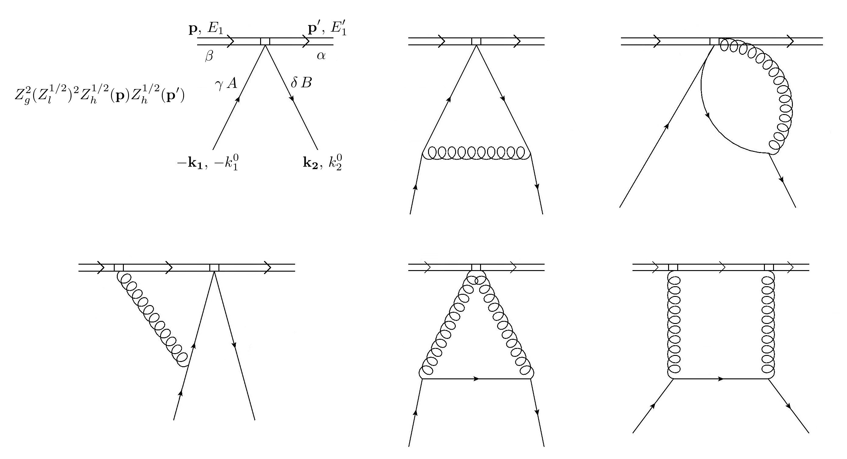
Figure 1: Topologies contributing to the LL running of Wilson coefficients associated to $1/m^{3}$ spin-dependent heavy-light operators. The first diagram is the tree level diagram multiplied by the renormalization of the external fields and coupling. The other diagrams are the one-loop topologies that also contribute. In general the depicted gluon can be either longitudinal or transverse. All possible vertices and insertions with the right counting in $1/m$ should be considered to generate the diagrams.

The RGE we obtain are

$$\nu\frac{d}{d\nu}d_{4}^{hl}=\frac{\alpha}{\pi}\bigg{[}(8C_{F}-3C_{A})\bigg{(}\frac{1}{32}c_{W_{1}}-\frac{1}{32}c_{W_{2}}+\frac{1}{16}c_{p^{\prime}p}+\frac{1}{64}c_{S}c_{k}$$

$$-\frac{1}{32}c_{S}c_{F}-\frac{5}{32}c_{F}c_{k}^{2}+\frac{5}{64}c_{F}^{2}c_{k}\bigg{)}-\frac{1}{4}d_{4}^{hl}(3C_{A}-2\beta_{0})\bigg{]}\,,$$ (35)

$$\nu\frac{d}{d\nu}d_{5}^{hl}=\frac{\alpha}{\pi}\bigg{[}C_{F}(2C_{F}-C_{A})\bigg{(}-\frac{1}{16}c_{W_{1}}+\frac{1}{16}c_{W_{2}}-\frac{1}{8}c_{p^{\prime}p}-\frac{1}{32}c_{S}c_{k}$$

$$+\frac{1}{16}c_{S}c_{F}+\frac{5}{16}c_{F}c_{k}^{2}-\frac{5}{32}c_{F}^{2}c_{k}\bigg{)}+\frac{1}{2}d_{5}^{hl}\beta_{0}\bigg{]}\,,$$ (36)

$$\nu\frac{d}{d\nu}d_{6}^{hl}=\frac{\alpha}{\pi}\bigg{[}\frac{1}{192}c_{B_{1}}C_{A}+\frac{1}{192}c_{S}c_{F}C_{A}-\frac{5}{96}c_{F}^{2}c_{k}C_{A}+\frac{1}{64}c_{2}^{hl}c_{F}(8C_{F}-3C_{A})+\frac{1}{16}c_{4}^{hl}c_{F}$$

$$+\frac{1}{3}d_{4}^{hl}(8C_{F}-3C_{A})+\frac{4}{3}d_{5}^{hl}+\frac{1}{6}d_{6}^{hl}(5C_{F}-5C_{A}+3\beta_{0})+\frac{5}{12}d_{8}^{hl}(2C_{F}-C_{A})+\frac{1}{12}d_{10}^{hl}C_{A}\bigg{]}\,,$$ (37)

$$\nu\frac{d}{d\nu}d_{7}^{hl}=\frac{\alpha}{\pi}\bigg{[}-C_{F}(2C_{F}-C_{A})\bigg{(}\frac{1}{32}c_{2}^{hl}c_{F}+\frac{2}{3}d_{4}^{hl}\bigg{)}+\frac{1}{6}d_{7}^{hl}(5C_{F}+3\beta_{0})+\frac{5}{6}d_{9}^{hl}C_{F}\bigg{]}\,,$$ (38)

$$\nu\frac{d}{d\nu}d_{8}^{hl}=\frac{\alpha}{\pi}\bigg{[}-\frac{1}{32}c_{W_{1}}C_{A}-\frac{1}{192}c_{B_{1}}C_{A}-\frac{1}{96}c_{B_{2}}C_{A}$$

$$-\frac{1}{64}c_{D}c_{F}C_{A}-\frac{1}{64}c_{S}c_{k}C_{A}+\frac{1}{192}c_{S}c_{F}C_{A}+\frac{5}{32}c_{F}c_{k}^{2}C_{A}-\frac{5}{96}c_{F}^{2}c_{k}C_{A}$$

$$-\frac{1}{64}c_{1}^{hl}c_{F}C_{A}-\frac{1}{16}c_{2}^{hl}c_{k}(8C_{F}-3C_{A})+\frac{1}{32}c_{2}^{hl}c_{F}(8C_{F}-3C_{A})-\frac{1}{4}c_{4}^{hl}c_{k}+\frac{1}{8}c_{4}^{hl}c_{F}$$

$$-\frac{1}{12}d_{4}^{hl}(8C_{F}-3C_{A})-\frac{1}{3}d_{5}^{hl}+\frac{1}{6}d_{6}^{hl}(3C_{F}-2C_{A})+\frac{1}{2}d_{8}^{hl}(C_{F}-2C_{A}+\beta_{0})+\frac{1}{6}d_{10}^{hl}C_{A}\bigg{]},\,$$ (39)

$$\nu\frac{d}{d\nu}d_{9}^{hl}=\frac{\alpha}{\pi}\bigg{[}C_{F}(2C_{F}-C_{A})\bigg{(}\frac{1}{8}c_{2}^{hl}c_{k}-\frac{1}{16}c_{2}^{hl}c_{F}+\frac{1}{6}d_{4}^{hl}\bigg{)}+\frac{1}{2}d_{7}^{hl}C_{F}+\frac{1}{2}d_{9}^{hl}(C_{F}+\beta_{0})\bigg{]},\,$$ (40)

$$\nu\frac{d}{d\nu}d_{10}^{hl}=\frac{\alpha}{\pi}\bigg{[}\frac{1}{48}c_{W_{1}}C_{A}+\frac{1}{192}c_{W_{2}}C_{A}-\frac{7}{192}c_{B_{1}}C_{A}-\frac{1}{48}c_{B_{2}}C_{A}+\frac{1}{384}c_{p^{\prime}p}C_{A}$$

$$+\frac{1}{128}c_{D}c_{F}C_{A}+\frac{1}{96}c_{S}c_{k}C_{A}-\frac{7}{384}c_{S}c_{F}C_{A}+\frac{5}{64}c_{F}^{2}c_{k}C_{A}$$

$$+\frac{1}{128}c_{1}^{hl}c_{F}C_{A}-\frac{1}{128}c_{2}^{hl}c_{F}(8C_{F}-3C_{A})-\frac{1}{32}c_{4}^{hl}c_{F}$$

$$+\frac{1}{24}d_{4}^{hl}(8C_{F}-3C_{A})+\frac{1}{6}d_{5}^{hl}-\frac{1}{24}d_{6}^{hl}(4C_{F}-3C_{A})$$

$$-\frac{1}{12}d_{8}^{hl}(2C_{F}-C_{A})-\frac{1}{24}d_{10}^{hl}(11C_{A}-12\beta_{0})\bigg{]}\,,$$ (41)

$$\nu\frac{d}{d\nu}d_{11}^{hl}=\frac{\alpha}{\pi}\bigg{[}C_{F}(2C_{F}-C_{A})\bigg{(}\frac{1}{64}c_{2}^{hl}c_{F}-\frac{1}{12}d_{4}^{hl}\bigg{)}-\frac{1}{6}d_{7}^{hl}C_{F}-\frac{1}{6}d_{9}^{hl}C_{F}+\frac{1}{2}d_{11}^{hl}\beta_{0}\bigg{]}\,.$$ (42)

The RGE of the remaining Wilson coefficients $d_{i}^{hl}$ have the structure ($i,j>11$)

$$\nu\frac{d}{d\nu}d_{i}^{hl}=\frac{\alpha}{\pi}A_{ij}d_{j}^{hl}\,.$$ (43)

And for this reason, they are NLL.

III.2 $1/m^{3}$ heavy quark bilinear operators: LL running of $c_{p^{\prime}p}$, $c_{Wi}$ and $c_{Bi}$

Let’s consider the $1/m^{3}$ spin-dependent operators bilinear in the heavy quark field of the HQET Lagrangian, namely, the running of the unphysical set: $\{c_{W_{1}},c_{W_{2}},c_{B_{1}},c_{B_{2}},c_{p^{\prime}p}\}$. The most difficult part of the work was already done in Ref. lmp . The only part which is left is the contribution due to heavy-light operators i.e. the running of these Wilson coefficients with $c_{i}^{hl},\,i=1,\ldots,4$ and $d_{i}^{hl},\,i=4,\ldots,11$. The procedure we use is the same that in Refs. chromopolarizabilities ; lmp . We compute the elastic scattering of a heavy quark with a transverse gluon only considering diagrams involving the vertices coming from $1/m^{2}$ and $1/m^{3}$ spin-dependent heavy-light operators. Diagrams are constructed from the topologies shown in Fig. 2 by considering all possible vertices and kinetic insertions to the appropriate order in $1/m$. Note that diagrams of lower order than $1/m^{3}$ also must be considered, as the use of the heavy quark EOM, $E=c_{k}\frac{{\bf p}^{2}}{2m}$, adds extra powers of $1/m$ in those terms which are proportional to the energy. The topologies drawn in Fig. 2 generate around 21 diagrams without taking into account permutations and crossing. The RGEs for the unphysical set $\{c_{W_{1}},c_{W_{2}},c_{B_{1}},c_{B_{2}},c_{p^{\prime}p}\}$, in Coulomb gauge, read

$$\nu\frac{d}{d\nu}c_{p^{\prime}p}=\gamma_{c_{p^{\prime}p},\,Q^{\dagger}Q}\,,$$ (44)

$$\nu\frac{d}{d\nu}c_{W_{1}}=\gamma_{c_{W_{1}},\,Q^{\dagger}Q}-\frac{\alpha}{\pi}T_{F}n_{f}\bigg{(}\frac{8}{3}d_{6}^{hl}-\frac{8}{3}d_{8}^{hl}+\frac{16}{3}d_{10}^{hl}\bigg{)}\,,$$ (45)

$$\nu\frac{d}{d\nu}c_{W_{2}}=\gamma_{c_{W_{2}},\,Q^{\dagger}Q}-\frac{\alpha}{\pi}T_{F}n_{f}\bigg{(}\frac{8}{3}d_{6}^{hl}-\frac{8}{3}d_{8}^{hl}+\frac{16}{3}d_{10}^{hl}\bigg{)}\,,$$ (46)

$$\nu\frac{d}{d\nu}c_{B_{1}}=\gamma_{c_{B_{1}},\,Q^{\dagger}Q}-\frac{\alpha}{\pi}T_{F}n_{f}\bigg{(}\frac{8}{3}d_{6}^{hl}-8d_{8}^{hl}+\frac{32}{3}d_{10}^{hl}\bigg{)}\,,$$ (47)

$$\nu\frac{d}{d\nu}c_{B_{2}}=\gamma_{c_{B_{2}},\,Q^{\dagger}Q}-\frac{\alpha}{\pi}T_{F}n_{f}\bigg{(}\frac{16}{3}d_{6}^{hl}+\frac{16}{3}d_{8}^{hl}\bigg{)}\,.$$ (48)

Where $\gamma_{c_{i},\,Q^{\dagger}Q}$ is the anomalous dimension of the Wilson coefficient $c_{i}$ found in Ref. lmp , that comes only from the terms of the HQET Lagrangian bilinear in the heavy quark field or, what is the same, it is the anomalous dimension for $n_{f}=0$.

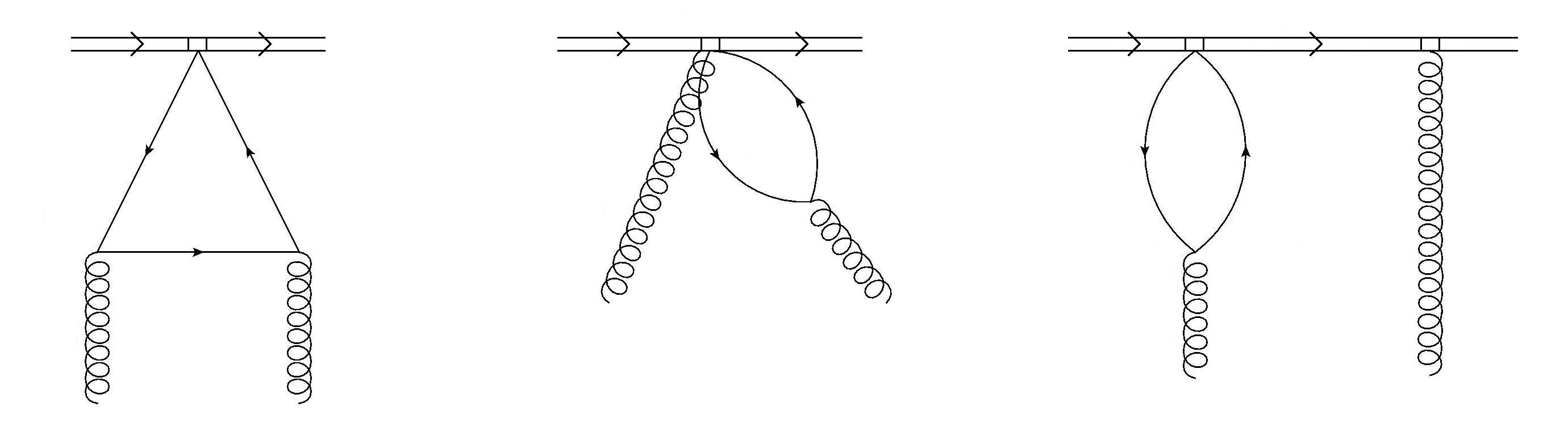
Figure 2: One loop topologies contributing to the anomalous dimensions of the Wilson coefficients of the $1/m^{3}$ operators bilinear in the heavy quark field. All diagrams are generated from these topologies by considering all possible vertices and kinetic insertions up to ${\cal O}(1/m^{3})$.

III.3 LL running of physical quantities

In the previous sections, Sec. III.1 and Sec. III.2, we found the running of the Wilson coefficients associated to the $1/m^{3}$ HQET Lagrangian operators including spectator quarks. However, it is well known from Ref. lmp that Eqs. (45)-(47) are not physical. So the next step, is to compute the RGEs for the the known physical quantities $\bar{c}_{W}=c_{W_{1}}-c_{W_{2}}$, $\bar{c}_{B_{1}}=c_{B_{1}}-2c_{W_{1}}$, $c_{B_{2}}$ and $c_{p^{\prime}p}$. They read

$$\nu\frac{d}{d\nu}c_{p^{\prime}p}=\gamma_{c_{p^{\prime}p},\,Q^{\dagger}Q}\,,$$ (49)

$$\nu\frac{d}{d\nu}\bar{c}_{W}=\gamma_{\bar{c}_{W},\,Q^{\dagger}Q}\,,$$ (50)

$$\nu\frac{d}{d\nu}\bar{c}_{B_{1}}=\gamma_{\bar{c}_{B_{1}},\,Q^{\dagger}Q}+\frac{8}{3}\bar{d}_{8}^{hl}T_{F}n_{f}\frac{\alpha}{\pi}\,,$$ (51)

$$\nu\frac{d}{d\nu}c_{B_{2}}=\gamma_{c_{B_{2}},\,Q^{\dagger}Q}-\frac{16}{3}\bar{d}_{8}^{hl}T_{F}n_{f}\frac{\alpha}{\pi}\,.$$ (52)

Note that Eqs. (49-50) satisfy the reparametrization invariant relations given in Ref. Manohar:1997qy , even with the inclusion of spectator quarks. From these equations we learn that $\bar{d}_{8}^{hl}=d_{6}^{hl}+d_{8}^{hl}$ must be physical as it appears in the running of physical combinations. Indeed, since the running of $d_{6}^{hl}$ and $d_{8}^{hl}$ can not be written in terms of gauge-independent quantities, $\bar{d}_{8}^{hl}$ must be a physical combination, whereas $d_{6}^{hl}$ and $d_{8}^{hl}$ alone are gauge dependent. The gauge independence of the RGE for $\bar{d}_{8}^{hl}$ also implies the existence of another physical combination, $\bar{d}_{10}^{hl}=8d_{6}^{hl}+8d_{10}^{hl}-c_{W_{1}}$, whose running also depends only on physical quantities, as expected. The running of these two physical combinations also depend on $d_{4}^{hl}$ and $d_{5}^{hl}$, which happen to be gauge independent, as their running only depend on physical quantities and on themselves, and they do not combine with any gauge dependent quantity in the running of gauge independent combinations. The Wilson coefficients $d_{7}^{hl}$, $d_{9}^{hl}$ and $d_{11}^{hl}$ do not mix with $c_{p^{\prime}p}$, $\bar{c}_{W}$, $\bar{c}_{B_{1}}$, $c_{B_{2}}$, $d_{4}^{hl}$, $d_{5}^{hl}$, $\bar{d}_{8}^{hl}$ and $\bar{d}_{10}^{hl}$, so they are not necessary to determine their running. Since they do not appear in known physical quantities we do not dare to talk about their gauge dependence. The RGEs for the physical set of light fermion Wilson coefficients read

$$\nu\frac{d}{d\nu}d_{4}^{hl}=\frac{\alpha}{\pi}\bigg{[}-\frac{1}{4}d_{4}^{hl}(3C_{A}-2\beta_{0})+(8C_{F}-3C_{A})\bigg{(}\frac{1}{32}\bar{c}_{W}+\frac{1}{16}c_{p^{\prime}p}$$

$$+\frac{1}{64}c_{S}c_{k}-\frac{1}{32}c_{S}c_{F}-\frac{5}{32}c_{F}c_{k}^{2}+\frac{5}{64}c_{F}^{2}c_{k}\bigg{)}\bigg{]}\,,$$ (53)

$$\nu\frac{d}{d\nu}d_{5}^{hl}=\frac{\alpha}{\pi}\bigg{[}\frac{1}{2}d_{5}^{hl}\beta_{0}+C_{F}(2C_{F}-C_{A})\bigg{(}-\frac{1}{16}\bar{c}_{W}-\frac{1}{8}c_{p^{\prime}p}$$

$$-\frac{1}{32}c_{S}c_{k}+\frac{1}{16}c_{S}c_{F}+\frac{5}{16}c_{F}c_{k}^{2}-\frac{5}{32}c_{F}^{2}c_{k}\bigg{)}\bigg{]}\,,$$ (54)

$$\nu\frac{d}{d\nu}\bar{d}_{8}^{hl}=\frac{\alpha}{\pi}\bigg{(}-\frac{1}{96}c_{B_{2}}C_{A}+\frac{1}{4}d_{4}^{hl}(8C_{F}-3C_{A})+d_{5}^{hl}+\frac{1}{12}\bar{d}_{8}^{hl}(16C_{F}-17C_{A}+6\beta_{0})$$

$$+\frac{1}{32}\bar{d}_{10}^{hl}C_{A}-\frac{1}{64}c_{S}c_{k}C_{A}+\frac{1}{96}c_{S}c_{F}C_{A}+\frac{5}{32}c_{F}c_{k}^{2}C_{A}-\frac{5}{48}c_{F}^{2}c_{k}C_{A}$$

$$-\frac{1}{64}\bar{c}_{1}^{hl}c_{F}C_{A}-\frac{1}{16}c_{2}^{hl}c_{k}(8C_{F}-3C_{A})+\frac{3}{64}c_{2}^{hl}c_{F}(8C_{F}-3C_{A})-\frac{1}{4}c_{4}^{hl}c_{k}+\frac{3}{16}c_{4}^{hl}c_{F}\bigg{)}\,,$$ (55)

$$\nu\frac{d}{d\nu}\bar{d}_{10}^{hl}=\frac{\alpha}{\pi}\bigg{(}-\frac{1}{24}c_{B_{2}}C_{A}+3d_{4}^{hl}(8C_{F}-3C_{A})+12d_{5}^{hl}+\frac{2}{3}\bar{d}_{8}^{hl}(8C_{F}-15C_{A}+3\beta_{0})$$

$$+\frac{35}{24}\bar{d}_{10}^{hl}C_{A}+\frac{13}{24}\bar{c}_{W}C_{A}-\frac{1}{48}c_{p^{\prime}p}C_{A}-\frac{5}{24}c_{S}c_{k}C_{A}+\frac{1}{16}c_{S}c_{F}C_{A}+\frac{1}{12}c_{F}c_{k}^{2}(16C_{F}+15C_{A})$$

$$-\frac{2}{3}c_{F}^{2}c_{k}C_{A}+\frac{1}{16}\bar{c}_{1}^{hl}c_{F}C_{A}+\frac{1}{16}c_{2}^{hl}c_{F}(8C_{F}-3C_{A})+\frac{1}{4}c_{4}^{hl}c_{F}\bigg{)}\,,$$ (56)

$$\nu\frac{d}{d\nu}d_{7}^{hl}=\frac{\alpha}{\pi}\bigg{(}-\frac{2}{3}d_{4}^{hl}C_{F}(2C_{F}-C_{A})+\frac{1}{6}d_{7}^{hl}(5C_{F}+3\beta_{0})+\frac{5}{6}d_{9}^{hl}C_{F}-\frac{1}{32}c_{2}^{hl}c_{F}C_{F}(2C_{F}-C_{A})\bigg{)}\,,$$ (57)

$$\nu\frac{d}{d\nu}d_{9}^{hl}=\frac{\alpha}{\pi}\bigg{(}\frac{1}{6}d_{4}^{hl}C_{F}(2C_{F}-C_{A})+\frac{1}{2}d_{7}^{hl}C_{F}+\frac{1}{2}d_{9}^{hl}(C_{F}+\beta_{0})$$

$$+\frac{1}{8}c_{2}^{hl}c_{k}C_{F}(2C_{F}-C_{A})-\frac{1}{16}c_{2}^{hl}c_{F}C_{F}(2C_{F}-C_{A})\bigg{)}\,,$$ (58)

$$\nu\frac{d}{d\nu}d_{11}^{hl}=\frac{\alpha}{\pi}\bigg{(}-\frac{1}{12}d_{4}^{hl}C_{F}(2C_{F}-C_{A})-\frac{1}{6}d_{7}^{hl}C_{F}-\frac{1}{6}d_{9}^{hl}C_{F}+\frac{1}{2}d_{11}^{hl}\beta_{0}+\frac{1}{64}c_{2}^{hl}c_{F}C_{F}(2C_{F}-C_{A})\bigg{)}\,.$$ (59)

Note that we include the Wilson coefficients $d_{7}^{hl}$, $d_{9}^{hl}$ and $d_{11}^{hl}$ despite of we do not know if they are physical or not. We do so because, we will solve also these RGEs in the next section, as it can be useful in the future. It it quite remarkable that the RGEs depend only on gauge-independent combinations of Wilson coefficients: $\bar{c}_{W}$, $\bar{c}_{B_{1}}$, $\bar{d}_{8}^{hl}$, $\bar{d}_{10}^{hl}$ and $\bar{c}_{1}^{hl}=c_{D}+c_{1}^{hl}$ (see Refs. Pineda:2001ra ; chromopolarizabilities for discussions about the last combination). This is a very strong check, as at intermediate steps we get contributions from $c_{W_{1}}$, $c_{W_{2}}$, $c_{B_{1}}$, $d_{6}^{hl}$, $d_{8}^{hl}$, $d_{10}^{hl}$, $c_{1}^{hl}$ and $c_{D}$, which only at the end of the computation arrange themselves in gauge-independent combinations.

The counterterm of each Wilson coefficient can be easily reconstructed from the RGEs knowing that the scaling with the renormalization scale is $\nu^{2\epsilon}$.

IV Solution and numerical analysis

We are only interested in the solution of the RGEs of gauge independent quantities, i.e. of those displayed in Sec. III.3. These RGEs can be rewritten in a compact form by defining a vector ${\bf A}=\{\bar{c}_{B_{1}},c_{B_{2}},d_{4}^{hl},d_{5}^{hl},\bar{d}_{8}^{hl},\bar{d}_{10}^{hl},d_{7}^{hl},d_{9}^{hl},d_{11}^{hl}\}$ (we do not include the RGEs of $c_{p^{\prime}p}$ and $\bar{c}_{W}$ because they are identical to the ones found in Ref. lmp , and were already solved in the same reference. Indeed, their solution can be easily found using the reparametrization invariant relations found in Ref. Manohar:1997qy . As pointed out in Sec. III.3, we do not know if the Wilson coefficients $d_{7}^{hl}$, $d_{9}^{hl}$ and $d_{11}^{hl}$ are physical or not, but we will solve their RGEs anyway). They read

$$\nu\frac{d{\bf A}}{d\nu}=\frac{\alpha}{\pi}({\bf M}{\bf A}+{\bf F}(\alpha))\,.$$ (60)

The matrix ${\bf M}$ and the vector ${\bf F}$ follow from the RGEs given in Sec. III.3. The running of the strong coupling constant, $\alpha$, is needed only with LL accuracy:

$$\nu{{\rm d\alpha}\over{\rm d}\nu}\equiv\beta(\alpha_{s})=-2\alpha\left\{\beta_{0}{\alpha\over 4\pi}+\cdots\right\}\,,$$ (61)

where

$$\beta_{0} = {11\over 3}C_{A}-{4\over 3}T_{F}n_{f}\,,$$ (62)

and $n_{f}$ is the number of dynamical (active) quarks i.e. the number of massless quarks.

In this approximation, the Eq. (60) can be simplified to

$$\frac{d{\bf A}}{d\alpha}=-\frac{2}{\beta_{0}\alpha}({\bf M}{\bf A}+{\bf F}(\alpha))\,.$$ (63)

It is more convenient to define $z\equiv\left(\frac{\alpha(\nu)}{\alpha(m)}\right)^{\frac{1}{\beta_{0}}}\simeq 1-\frac{1}{2\pi}\alpha(\nu)\ln(\frac{\nu}{m})$ and rewrite the equation above as:

$$\frac{d{\bf A}}{dz}=-\frac{2}{z}(\mathbf{M}{\bf A}+{\bf F}(z))\,.$$ (64)

In order to solve Eq. 64, we need the initial matching conditions at the hard scale, at tree-level. For the bilinear sector, they have been determined in Ref. Manohar:1997qy and read $c_{k}=c_{F}=c_{D}=c_{S}=c_{W_{1}}=c_{B_{1}}=1$ and $c_{W_{2}}=c_{p^{\prime}p}=c_{B_{2}}=0$. There are no tree level contribution to the Wilson coefficients associated to heavy-light operators, so its initial matching conditions are $c_{i}^{hl}=0,\,i=1,\ldots 4$ and $d_{i}^{hl}=0,\,i=4,\ldots,11$. The Wilson coefficients $c_{k}$, $c_{F}$, $c_{S}=2c_{F}-1$, $c_{p^{\prime}p}=c_{F}-1$, $\bar{c}_{W}=1$, $\bar{c}_{1}^{hl}$, $c_{2}^{hl}$, $c_{3}^{hl}$ and $c_{4}^{hl}$ are needed with LL accuracy. They can be found in Refs. Pineda:2011dg ; Manohar:1997qy ; Bauer:1997gs

After solving the RGEs we obtain the LL running of the Wilson coefficients associated to the $1/m^{3}$ spin-dependent operators of the HQET Lagrangian including spectator quark effects. The solution is numerical and reads

$$\bar{c}_{B_{1}}=-0.695+\frac{0.045788}{z^{11.333333}}+\frac{13.6766}{z^{9.762121}}-\frac{10.4869}{z^{9}}+\frac{0.0690}{z^{8.333333}}-\frac{0.3586}{z^{8.24892}}$$

$$-\frac{1.83813}{z^{6.833333}}+\frac{1.34179}{z^{6.549986}}+\frac{1}{z^{6}}+\frac{4.49328}{z^{3.833333}}-\frac{4.95805}{z^{3.577865}}-\frac{3.290}{z^{3}}\,,$$ (65)

$$c_{B_{2}}=-2.966-\frac{0.065821}{z^{11.333333}}-\frac{16.4471}{z^{9.762121}}+\frac{13.4869}{z^{9}}-\frac{0.0493}{z^{8.333333}}+\frac{0.2388}{z^{8.24892}}$$

$$-\frac{2.94100}{z^{6.833333}}+\frac{4.6355}{z^{6.549986}}-\frac{4.3137}{z^{6}}-\frac{15.2080}{z^{3.833333}}+\frac{16.0570}{z^{3.577865}}+\frac{7.572}{z^{3}}\,,$$ (66)

$$d_{4}^{hl}=0.0407609-\frac{3.203\cdot 10^{-23}}{z^{11.333333}}-\frac{3.9035\cdot 10^{-21}}{z^{9.5}}-\frac{5.1587\cdot 10^{-22}}{z^{9}}+\frac{7.87\cdot 10^{-22}}{z^{8.333333}}$$

$$+\frac{3.053\cdot 10^{-21}}{z^{8.24892}}+\frac{2.2581\cdot 10^{-21}}{z^{6.833333}}+\frac{3.8386\cdot 10^{-23}}{z^{6.549986}}+\frac{0.024038462}{z^{6}}$$

$$-\frac{0.1897993}{z^{3.833333}}+\frac{1.97644\cdot 10^{-20}}{z^{3.577865}}+\frac{0.125}{z^{3}}\,,$$ (67)

$$d_{5}^{hl}=0.01-\frac{2.22704\cdot 10^{-22}}{z^{11.333333}}-\frac{5.46119\cdot 10^{-20}}{z^{9.762121}}+\frac{1.24130\cdot 10^{-21}}{z^{9.5}}+\frac{4.30351\cdot 10^{-20}}{z^{9}}$$

$$-\frac{0.00851190}{z^{8.333333}}+\frac{3.836\cdot 10^{-23}}{z^{8.24892}}+\frac{1.10836\cdot 10^{-21}}{z^{6.833333}}-\frac{9.1837\cdot 10^{-23}}{z^{6.549986}}$$

$$-\frac{0.01190476}{z^{6}}+\frac{5.1030\cdot 10^{-22}}{z^{3.833333}}-\frac{1.84872\cdot 10^{-21}}{z^{3.577865}}+\frac{0.0104167}{z^{3}}\,,$$ (68)

$$\bar{d}_{8}^{hl}=-0.1149+\frac{0.0069309}{z^{11.333333}}+\frac{0.206216}{z^{9.762121}}-\frac{0.211554}{z^{9}}-\frac{0.00663}{z^{8.333333}}+\frac{0.03645}{z^{8.24892}}$$

$$+\frac{0.235510}{z^{6.833333}}-\frac{0.090907}{z^{6.549986}}-\frac{0.24908}{z^{6}}-\frac{2.88931}{z^{3.833333}}+\frac{3.27297}{z^{3.577865}}-\frac{0.1957}{z^{3}}\,,$$ (69)

$$\bar{d}_{10}^{hl}=-0.851-\frac{0.000658}{z^{11.333333}}+\frac{1.52703}{z^{9.762121}}-\frac{1.3162}{z^{9.5}}-\frac{1.39575}{z^{9}}+\frac{0.2628}{z^{8.333333}}+\frac{1.024}{z^{8.24892}}$$

$$+\frac{0.81541}{z^{6.833333}}+\frac{0.0125353}{z^{6.549986}}-\frac{0.1392}{z^{6}}-\frac{7.7003}{z^{3.833333}}+\frac{8.65108}{z^{3.577865}}-\frac{1.890}{z^{3}}\,,$$ (70)

$$d_{7}^{hl}=-0.000867+\frac{0.0000799}{z^{11.888889}}+\frac{3.346\cdot 10^{-24}}{z^{11.333333}}+\frac{4.0769\cdot 10^{-22}}{z^{9.5}}+\frac{0.020957}{z^{9}}$$

$$-\frac{0.036600}{z^{8.333333}}-\frac{3.188\cdot 10^{-22}}{z^{8.24892}}+\frac{0.01792}{z^{6.833333}}-\frac{4.0091\cdot 10^{-24}}{z^{6.549986}}$$

$$-\frac{0.000611}{z^{6}}-\frac{0.00086}{z^{3.833333}}-\frac{2.06422\cdot 10^{-21}}{z^{3.577865}}-\frac{0.00002}{z^{3}}\,,$$ (71)

$$d_{9}^{hl}=-0.006752+\frac{0.0000479}{z^{11.888889}}-\frac{1.5783\cdot 10^{-24}}{z^{11.333333}}-\frac{1.9232\cdot 10^{-22}}{z^{9.5}}-\frac{0.009862}{z^{9}}$$

$$+\frac{0.036600}{z^{8.333333}}+\frac{1.504\cdot 10^{-22}}{z^{8.24892}}-\frac{0.067979}{z^{6.833333}}+\frac{1.89125\cdot 10^{-24}}{z^{6.549986}}$$

$$+\frac{0.019841}{z^{6}}+\frac{0.05322}{z^{3.833333}}+\frac{9.7377\cdot 10^{-22}}{z^{3.577865}}-\frac{0.025117}{z^{3}}\,,$$ (72)

$$d_{11}^{hl}=-0.000769-\frac{0.00001598}{z^{11.888889}}+\frac{7.019\cdot 10^{-25}}{z^{11.333333}}+\frac{8.553\cdot 10^{-23}}{z^{9.5}}+\frac{0.0006164}{z^{9}}$$

$$-\frac{0.006880}{z^{8.333333}}-\frac{6.69\cdot 10^{-23}}{z^{8.24892}}+\frac{0.013287}{z^{6.833333}}-\frac{8.4104\cdot 10^{-25}}{z^{6.549986}}$$

$$-\frac{0.009005}{z^{6}}+\frac{0.008295}{z^{3.833333}}-\frac{4.33038\cdot 10^{-22}}{z^{3.577865}}-\frac{0.005529}{z^{3}}\,.$$ (73)

The single log results can be found analytically by solving Eqs. (53)-(59) just taking the tree level values of the Wilson coefficients that appear and considering $\alpha$ as a constant. We do not present the single log result of $\bar{c}_{B_{1}}$ and $c_{B_{2}}$ because spectators do not affect them, as their matching conditions are zero, and they were already found in Ref. lmp . For the Wilson coefficients associated to heavy-light operators we obtain

$$d_{4}^{hl}=-\frac{1}{16}(8C_{F}-3C_{A})\frac{\alpha}{\pi}\ln\left(\frac{\nu}{m}\right)+\mathcal{O}(\alpha^{2})\,,$$ (74)

$$d_{5}^{hl}=\frac{1}{8}C_{F}(2C_{F}-C_{A})\frac{\alpha}{\pi}\ln\left(\frac{\nu}{m}\right)+\mathcal{O}(\alpha^{2})\,,$$ (75)

$$\bar{d}_{8}^{hl}(\nu)=\mathcal{O}(\alpha^{2})\,,$$ (76)

$$\bar{d}_{10}^{hl}=-1+\left(\frac{4}{3}C_{F}-\frac{5}{12}C_{A}\right)\frac{\alpha}{\pi}\ln\left(\frac{\nu}{m}\right)+\mathcal{O}(\alpha^{2})\,,$$ (77)

$$d_{7}^{hl}=\mathcal{O}(\alpha^{2})\,,$$ (78)

$$d_{9}^{hl}=\mathcal{O}(\alpha^{2})\,,$$ (79)

$$d_{11}^{hl}=\mathcal{O}(\alpha^{2})\,.$$ (80)

Note that $\bar{d}_{8}^{hl}$ and $d_{i}^{hl},\,i=7,9,11$, are zero at the level of the single log. This means that the first contribution will be of $\mathcal{O}(\alpha^{2}\ln^{2}(\nu/m))$ and, as a consequence, their running will be small compared to the other Wilson coefficients because the single log dominates the expansion in the strong coupling, $\alpha$.

Spectator effects in HQET up to $\mathcal{O}(1/m^{3})$ were already studied in Ref. Balzereit:1998am . However, no anomalous dimension matrix for the Wilson coefficients was given, but only the single log expressions. At this level, we can compare our results with the ones given in that reference. The first thing we observe is that, in Ref. Balzereit:1998am , it is stated that spin-dependent heavy-light operators change the single log results of the bilinear sector already found in Ref. Balzereit:1998jb . That is strange, because the initial matching conditions of heavy-light operators is zero, and therefore, they should not change the single log expressions. After a more detailed comparison, taking the single logs given in Ref. Balzereit:1998am and using Eqs.(47)-(51) of Ref. lmp to change the operator basis, we find that, for physical combinations, the single log results remain unchanged and are still in agreement with Ref. lmp and with what we find in this paper (that single logs remain unchanged including spectators). Concerning the running of heavy-light operators, we find that $c_{7+}^{(3h)o}=c_{7-}^{(3h)o}=8d_{4}^{hl}$. The first equality is already in disagreement with Ref. Balzereit:1998am , and for the explicit single logs given in it, only the term proportional to $C_{F}$ agrees with ours. We also find that $c_{7+}^{(3h)s}=c_{7-}^{(3h)s}=8d_{5}^{hl}$, which leads to agreement between the single logs presented in Ref. Balzereit:1998am and ours. Also the given results for $d_{7}^{hl}$, $d_{9}^{hl}$ and $d_{11}^{hl}$ are in agreement. We find that $c_{6-}^{(3l)o}+c_{7-}^{(3l)o}=8\bar{d}_{8}^{hl}$, which also agrees. Finally, we find that $\bar{d}_{10}^{hl}=c_{6}^{(3l)o}-(c_{7+}^{(3h)o}-c_{7-}^{(3h)o})/2-c_{W_{1}}^{FG}$ (where $c_{W_{1}}^{FG}$ is the Wilson coefficient $c_{W_{1}}$ evaluated in the Feynman gauge, whose single log expression was found in Ref. Balzereit:1998jb ), for which we find disagreement (even though a change of sign in the single log of $c_{6}^{(3l)o}$ plus the condition $c_{7+}^{(3h)o}=c_{7-}^{(3h)o}$, expected to reproduce $d_{4}^{hl}$ correctly, would lead to agreement. This also would imply a change of sign in the single log expression of $c_{7-}^{(3l)o}$).

In Figs. 3, 4 we plot the results ontained in Sec. IV applied to the bottom heavy quark case, ilustrating the importance of incorporating large logarithms in heavy quark physics. Only physical combinations and specific combinations that appear in physical observables, like Compton scattering (see Ref. lmp ), are represented. We run the Wilson coefficients from the heavy quark mass to 1 GeV. For illustrative purposes, we take $m_{b}=4.73$ GeV and $\alpha(m_{b})=0.215943$.

Concerning the numerical analysis, we observe that spector quarks change slighly the running of the physical quantities computed in Ref. lmp , $\bar{c}_{B_{1}}$ and $c_{B_{2}}$, but that change is small (of approximately $0.1$ after running, with respect to the LL result with $n_{f}=0$, when they have a value of $\sim-2$ and $\sim 1$, respectively), so the effect induced by them is numerically subleading. However, the effect induced by the spectators tends to get away the curve from the single log one, so it makes the resummation of large logs more important. The change in combinations that appear in Compton scattering, like $\bar{c}_{B_{1}}+c_{B_{2}}$ is sizable, but even smaller than before. It changes by $0.02$ after running with respect to the LL result with $n_{f}=0$. Concerning the Wilson coefficients associated to heavy-light operators, we find that their running is small but sizable in some cases. The running is saturated by the single log in $d_{4}^{hl}$, $d_{5}^{hl}$ and $\bar{d}_{10}^{hl}$. In particular, $d_{4}^{hl}$ changes from $0$ to $0.012$ after running, and differs from the single log by $0.001$, $d_{5}^{hl}$ changes from $0$ to $0.006$. In that case, the resumation of logs happens to be unimportant. In the case of $\bar{d}_{10}^{hl}$, the resummation of logs introduces a difference of $\sim 0.015$ at $1$ GeV, with respect to the single log value. The Wilson coefficient runs from $-1$ to $-1.042$. The resumation of logs happens to be qualitatively very important for $\bar{d}_{8}^{hl}$, $d_{7}^{hl}$, $d_{9}^{hl}$ and $d_{11}^{hl}$, even though their running is small, because their behaviour is not saturated by the single log. They go from $0$ to $8.2\cdot 10^{-4}$, $-3\cdot 10^{-5}$, $-1.5\cdot 10^{-4}$ and $-5\cdot 10^{-5}$, respectively, after running at $\sim 1.5$ GeV.

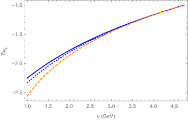
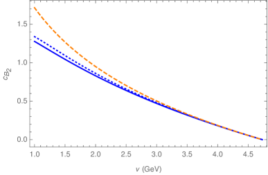
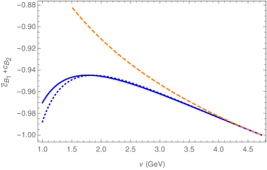
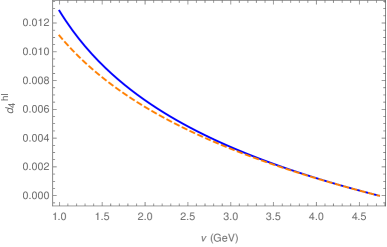
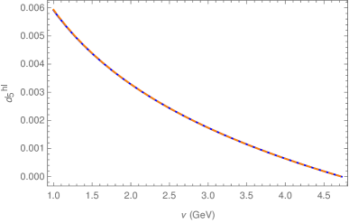
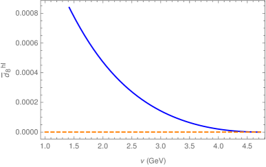
Figure 3: Running of the $1/m^{3}$ spin-dependent Wilson coefficients: $\bar{c}_{B_{1}}$, $c_{B_{2}}$, $\bar{c}_{B_{1}}+c_{B_{2}}$, $d_{4}^{hl}$, $d_{5}^{hl}$ and $\bar{d}_{8}^{hl}$, applied to the bottom heavy quark case. The continuous line is the LL result with $n_{f}=4$, the dotted line is the LL result with $n_{f}=0$ and the dashed line is the single leading logarithmic result (it does not depend on $n_{f}$).

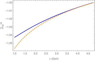
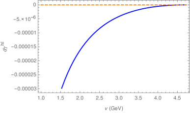
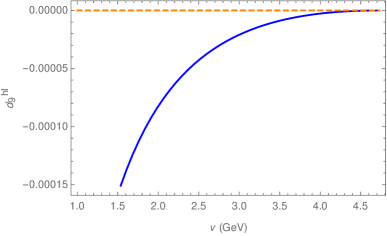
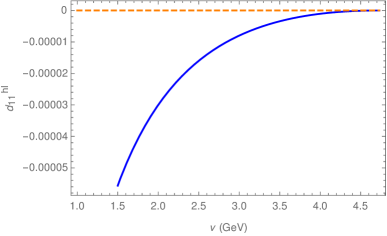
Figure 4: Running of the $1/m^{3}$ spin-dependent Wilson coefficients: $\bar{d}_{10}^{hl}$, $d_{7}^{hl}$, $d_{9}^{hl}$ and $d_{11}^{hl}$, applied to the bottom heavy quark case. The continuous line is the LL result with $n_{f}=4$ and the dashed line is the single leading logarithmic result (it does not depend on $n_{f}$).

V Conclusions

We have obtained, for the first time, the LL running of the Wilson coefficients associated to the $1/m^{3}$ spin-dependent heavy-light operators of the HQET Lagrangian, and their mixing with the Wilson coefficients associated to the $1/m^{3}$ spin-dependent operators bilinear in the heavy quark fields. It has been observed that, spectator quark effects are numerically subleading with respect to the ones coming from the bilinear sector. It has been proven that, after the inclusion of massless fermions, the relations coming from reparametrization invariance Manohar:1997qy are still satisfied and that the running of physical quantities depends only on gauge-independent quantities, as expected. Even though spectator effects are found to be numerically subleading, they have to be included, formally.

The presented results are written in a more standard basis, set by Ref. Manohar:1997qy , than the one used previously by Refs. Balzereit:1998am ; Balzereit:1998jb ; Balzereit:1998vh , and they are connected more closely to observables, as the quantities computed here are gauge independent. We have compared our results with the previous work done in Refs. Balzereit:1998jb ; Balzereit:1998am . For the gauge invariant combinations we have computed in our paper, the single logs presented in these references are in agreement with ours, except for $d_{4}^{hl}$ and $\bar{d}_{10}^{hl}$.

The Wilson coefficients computed in this paper could have many applications in heavy quark and heavy quarkonium physics. In particular, they are necessary ingredients to obtain the pNRQCD Lagrangian with next-to-next-to-next-to-next-to-leading order (NNNNLO) and with next-to-next-to-next-to-next-to-leading logarithmic (NNNNLL) accuracy, which is the necessary precision to determine the $\mathcal{O}(m\alpha^{6})$ and the $\mathcal{O}(m\alpha^{7}\ln\alpha+m\alpha^{8}\ln^{2}\alpha+\ldots)$ heavy quarkonium spectrum. They also have applications in QED bound states like in muonic hydrogen.

Acknowledgments
We thank Antonio Pineda for reading over the manuscript. This work was supported by the Spanish grants FPA2014-55613-P, FPA2017-86989-P and SEV-2016-0588.

Appendix A HQET Feynman rules

Here we collect the new and necessary Feynman rules associated to the $1/m^{3}$ spin-dependent heavy-light operators given in Eqs. (27)-(34), and that complement those that can be found in Refs. Pineda:2011dg ; chromopolarizabilities . The conventions are shown in Fig. 5.

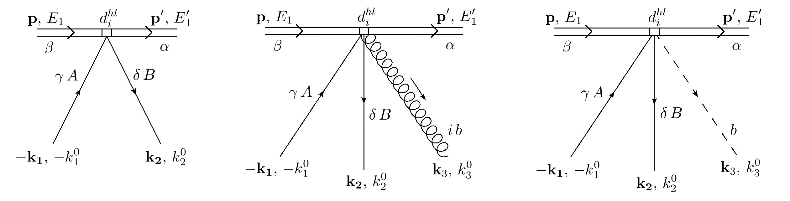
Figure 5: Conventions for Feynman rules involving spin-dependent heavy-light operators which get LL runing. The double line represents a heavy quark, the single line a massless quark, and the curly and dashed lines represent a tranverse and longitudinal gluon respectively. The index $i$ goes from 4 to 11.

A.1 Proportional to $d_{4}^{hl}$

$$\mathcal{V}=-d_{4}^{hl}\frac{ig^{2}}{m^{3}}(\gamma^{0}\gamma_{5})_{BA}(T^{a})_{\alpha\beta}(T^{a})_{\delta\gamma}\mbox{\boldmath$\sigma$}\cdot({\bf p}+{\bf p}^{\prime})$$ (81)

$$\mathcal{V}^{i\,b}=d_{4}^{hl}\frac{ig^{3}}{m^{3}}(\gamma^{0}\gamma_{5})_{BA}(T^{a})_{\delta\gamma}\{T^{a},T^{b}\}_{\alpha\beta}\mbox{\boldmath$\sigma$}^{i}$$ (82)

A.2 Proportional to $d_{5}^{hl}$

$$\mathcal{V}=-d_{5}^{hl}\frac{ig^{2}}{m^{3}}(\gamma^{0}\gamma_{5})_{BA}(I_{N_{c}})_{\alpha\beta}(I_{N_{c}})_{\delta\gamma}\mbox{\boldmath$\sigma$}\cdot({\bf p}+{\bf p}^{\prime})$$ (83)

$$\mathcal{V}^{i\,b}=d_{5}^{hl}\frac{2ig^{3}}{m^{3}}(\gamma^{0}\gamma_{5})_{BA}(I_{N_{c}})_{\delta\gamma}(T^{b})_{\alpha\beta}\mbox{\boldmath$\sigma$}^{i}$$ (84)

A.3 Proportional to $d_{6}^{hl}$

$$\mathcal{V}=d_{6}^{hl}\frac{ig^{2}}{m^{3}}(\gamma^{0}\gamma_{5})_{BA}(T^{a})_{\alpha\beta}(T^{a})_{\delta\gamma}\mbox{\boldmath$\sigma$}\cdot({\bf k}_{1}-{\bf k}_{2})$$ (85)

$$\mathcal{V}^{i\,b}=d_{6}^{hl}\frac{ig^{3}}{m^{3}}(\gamma^{0}\gamma_{5})_{BA}\{T^{a},T^{b}\}_{\delta\gamma}(T^{a})_{\alpha\beta}\mbox{\boldmath$\sigma$}^{i}$$ (86)

A.4 Proportional to $d_{7}^{hl}$

$$\mathcal{V}=d_{7}^{hl}\frac{ig^{2}}{m^{3}}(\gamma^{0}\gamma_{5})_{BA}(I_{N_{c}})_{\alpha\beta}(I_{N_{c}})_{\delta\gamma}\mbox{\boldmath$\sigma$}\cdot({\bf k}_{1}-{\bf k}_{2})$$ (87)

$$\mathcal{V}^{i\,b}=d_{7}^{hl}\frac{2ig^{3}}{m^{3}}(\gamma^{0}\gamma_{5})_{BA}(T^{b})_{\delta\gamma}(I_{N_{c}})_{\alpha\beta}\mbox{\boldmath$\sigma$}^{i}$$ (88)

A.5 Proportional to $d_{8}^{hl}$

$$\mathcal{V}=d_{8}^{hl}\frac{ig^{2}}{m^{3}}(\gamma^{i}\gamma_{5})_{BA}(T^{a})_{\alpha\beta}(T^{a})_{\delta\gamma}\mbox{\boldmath$\sigma$}^{i}(k_{1}^{0}-k_{2}^{0})$$ (89)

$$\mathcal{V}^{b}=d_{8}^{hl}\frac{ig^{3}}{m^{3}}(\gamma^{i}\gamma_{5})_{BA}\{T^{a},T^{b}\}_{\delta\gamma}(T^{a})_{\alpha\beta}\mbox{\boldmath$\sigma$}^{i}$$ (90)

A.6 Proportional to $d_{9}^{hl}$

$$\mathcal{V}=d_{9}^{hl}\frac{ig^{2}}{m^{3}}(\gamma^{i}\gamma_{5})_{BA}(I_{N_{c}})_{\alpha\beta}(I_{N_{c}})_{\delta\gamma}\mbox{\boldmath$\sigma$}^{i}(k_{1}^{0}-k_{2}^{0})$$ (91)

$$\mathcal{V}^{b}=d_{9}^{hl}\frac{2ig^{3}}{m^{3}}(\gamma^{i}\gamma_{5})_{BA}(T^{b})_{\delta\gamma}(I_{N_{c}})_{\alpha\beta}\mbox{\boldmath$\sigma$}^{i}$$ (92)

A.7 Proportional to $d_{10}^{hl}$

$$\mathcal{V}=d_{10}^{hl}\frac{g^{2}}{m^{3}}(T^{a})_{\alpha\beta}(T^{a})_{\delta\gamma}(\gamma^{i})_{BA}(\mbox{\boldmath$\sigma$}\times{\bf k})^{i}$$ (93)

$$\mathcal{V}^{i\,b}=d_{10}^{hl}\frac{g^{3}}{m^{3}}(\gamma^{j})_{BA}[T^{a},T^{b}]_{\delta\gamma}(T^{a})_{\alpha\beta}\epsilon^{ijk}\mbox{\boldmath$\sigma$}^{k}$$ (94)

A.8 Proportional to $d_{11}^{hl}$

$$\mathcal{V}=d_{11}^{hl}\frac{g^{2}}{m^{3}}(I_{N_{c}})_{\alpha\beta}(I_{N_{c}})_{\delta\gamma}(\gamma^{i})_{BA}(\mbox{\boldmath$\sigma$}\times{\bf k})^{i}$$ (95)

References

(1) M.B. Voloshin and M.A. Shifman, Sov. J. Nucl. Phys.
45, 292 (1987); H.D. Politzer and M.B. Wise, Phys. Lett. B 206, 681 (1988); N. Isgur and M. B. Wise, Phys. Lett. B 232, 113
(1989); E. Eichten and B. Hill, Phys. Lett. B 234, 511 (1990);
H. Georgi, Phys. Lett. B 240, 447 (1990); B. Grinstein,
Nucl. Phys. B339, 253 (1990).
(2) W.E. Caswell and G.P. Lepage, Phys. Lett.167B, 437
(1986).
(3)
G. T. Bodwin, E. Braaten and G. P. Lepage,
Phys. Rev. D 51, 1125 (1995)
Erratum: [Phys. Rev. D 55, 5853(E) (1997)].
[hep-ph/9407339].
(4)
A. Pineda and J. Soto,
Nucl. Phys. Proc. Suppl. 64, 428 (1998).
[hep-ph/9707481].
(5)
N. Brambilla, A. Pineda, J. Soto and A. Vairo,
Nucl. Phys. B566, 275 (2000).
[hep-ph/9907240].
(6)
N. Brambilla, A. Pineda, J. Soto and A. Vairo,
Rev. Mod. Phys. 77, 1423 (2005).
[hep-ph/0410047].
(8)
X. Lobregat, D. Moreno and R. Petrossian-Byrne,
Phys. Rev. D 97, 054018 (2018).
[hep-ph/1802.07767].
(9)
A. A. Penin, A. Pineda, V. A. Smirnov and M. Steinhauser,
Nucl. Phys. B699 (2004) 183-206
Erratum: [Nucl. Phys. B829 (2010) 398-399].
[hep-ph/0406175].
(10)
C. Anzai, D. Moreno, A. Penin, A. Pineda and M. Steinhauser (to be published).
(11)
A. V. Manohar,
Phys. Rev. D 56, 230 (1997).
[hep-ph/9701294].
(12)
C. Balzereit,
Phys. Rev. D 59, 094015 (1999).
[hep-ph/9805503].
(13)
M. Finkemeier and M. McIrvin,
Phys. Rev. D 55, 377 (1997).
[hep-ph/9607272].
(14)
B. Blok, J. G. Korner, D. Pirjol and J. C. Rojas,
Nucl. Phys. B496, 358 (1997).
[hep-ph/9607233].
(15)
C. W. Bauer and A. V. Manohar,
Phys. Rev. D 57, 337 (1998).
[hep-ph/9708306].
(16)
C. Balzereit,
Phys. Rev. D 59, 034006 (1999).
[hep-ph/9801436].
(17)
C. Balzereit,
arXiv: hep-ph/9809226.
(18)
D. Moreno and A. Pineda,
Phys. Rev. D 97, 016012 (2018).
[hep-ph/1710.07647].
(19)
M. E. Luke and A. V. Manohar,
Phys. Lett. B 286, 348 (1992).
[arXiv:hep-ph/9205228].
(20)
A. Pineda, Phys. Rev. D 65, 074007 (2002).
[hep-ph/0109117].