Fermi surface pockets in electron-doped iron superconductor by Lifshitz transition

Abstract

The Fermi surface pockets that lie at the corner of the two-iron Brillouin zone in heavily electron-doped iron selenide superconductors are accounted for by an extended Hubbard model over the square lattice of iron atoms that includes the principal $3d_{xz}$ and $3d_{yz}$ orbitals. At half filling, and in the absence of intra-orbital next-nearest neighbor hopping, perfect nesting between electron-type and hole-type Fermi surfaces at the the center and at the corner of the one-iron Brillouin zone is revealed. It results in hidden magnetic order in the presence of magnetic frustration within mean field theory. An Eliashberg-type calculation that includes spin-fluctuation exchange finds that the Fermi surfaces undergo a Lifshitz transition to electron/hole Fermi surface pockets centered at the corner of the two-iron Brillouin zone as on-site repulsion grows strong. In agreement with angle-resolved photoemission spectroscopy on iron selenide high-temperature superconductors, only the two electron-type Fermi surface pockets remain after a rigid shift in energy of the renormalized band structure by strong enough electron doping. At the limit of strong on-site repulsion, a spin-wave analysis of the hidden-magnetic-order state finds a “floating ring” of low-energy spin excitations centered at the checkerboard wavenumber $(\pi,\pi)$. This prediction compares favorably with recent observations of low-energy spin resonances around $(\pi,\pi)$ in intercalated iron selenide by inelastic neutron scattering.

1 Introduction

The family of iron-based superconductors first discovered ten years ago has established a new route to high critical temperatures[1]. In particular, stoichiometric FeSe becomes superconducting below a modest critical temperature of $8$ K. Electron doping of FeSe raises the critical temperature dramatically into the range $40$-$110$ K, however[2, 3]. The latter has been achieved by laying a monolayer of FeSe over a substrate[4, 5, 6, 7], by intercalating layers of FeSe with organic compounds[8, 9, 10], by dosing thin films of FeSe with alkali metals[11, 12, 13], and by applying a gate voltage to thin films of FeSe[14, 15]. Angle-resolved photoemission spectroscopy (ARPES) on such heavily electron-doped FeSe reveals two electron-type Fermi surface pockets at the corner of the two-iron Brillouin zone[5, 6]. It also reveals buried hole bands at the center of the two-iron Brillouin zone that lie $60$ meV below the bottom of the former electron bands[8, 16]. At low temperature, ARPES also finds an isotropic gap at the electron Fermi surface pockets consistent with a superconducting state[8, 17]. The energy gap at the Fermi surface is confirmed by scanning tunneling microscopy on heavily electron-doped FeSe[7, 10, 13]. By comparison with stoichiometric FeSe, which has a relatively low critical temperature, it has been argued that the phenomenon of high-temperature superconductivity in heavily electron-doped FeSe is due to the appearance of a new electronic groundstate[18, 19].

In addition, recent inelastic neutron scattering experiments on intercalated FeSe find a ring of low-energy magnetic excitations centered at the wave number $(\pi/a,\pi/a)$ associated with Néel order over the square lattice of iron atoms in a single layer[20, 21, 22]. Here, $a$ denotes the lattice constant. It has been suggested recently by one of the authors that this ring of low-energy magnetic excitations is a result of hidden Néel order among the iron $3d$ orbitals[18, 23]. (See Fig. 6.) Such hidden magnetic order can emerge because of frustration among local magnetic moments over the square lattice of iron atoms in FeSe[24, 25]. One of the authors has shown that adding electrons to the local magnetic moments at half filling results in electron-type Fermi surface pockets at the corner of the two-iron Brillouin zone, but with no Fermi surface at the center[18]. It is important to mention, at this stage, that conventional band structure calculations for electron-doped FeSe typically predict additional hole-type Fermi surface pockets at the center of the two-iron Brillouin zone, in marked contrast to ARPES measurements[8, 17, 26]

In this paper, we shall introduce an extended Hubbard model over the square lattice of iron atoms in heavily electron-doped FeSe that harbors hidden Néel order among the $3d_{xz}/3d_{yz}$ orbitals because of perfect nesting of electron-type and of hole-type Fermi surfaces at the center and at the corner of the one-iron Brillouin zone, with nesting wavenumber $(\pi/a,\pi/a)$. True Néel order is suppressed because of magnetic frustration from super-exchange interactions across the Se atoms[24, 25]. At half filling, mean field theory similar to that for the one-orbital Hubbard model over the square lattice[27] finds a stable hidden spin-density wave (hSDW) at the same wavenumber, but with a nodal $D_{xy}$ gap in the quasi-particle spectrum at the Fermi surface. Also in analogy with the one-orbital Hubbard model over the square lattice[28, 29, 30], we identify two collective modes of the mean field theory that represent spin-wave excitations of the hSDW. They vanish in energy at the Néel wave number $(\pi/a,\pi/a)$ with an acoustic dispersion. We argue in the Discussion section that degeneracy of these hidden Goldstone modes with true spin excitations results in a ring of low-energy magnetic excitations similar to what is observed by inelastic neutron scattering in intercalated FeSe[20, 21, 22].

Next, we shall formulate an Eliashberg theory[31, 32, 33] for the extended Hubbard model of  a single layer of heavily electron-doped FeSe that is based on exchange of the above hidden spin-wave excitations by electrons and by holes (particle-hole channel). A solution of the associated Eliashberg equations[34] finds a Lifshitz transition of the electron/hole Fermi surfaces to pockets centered at the corner of the two-iron Brillouin zone at moderate to strong on-site Coulomb repulsion. This result is consistent with similar results obtained by one of the authors at the limit of strong on-site Coulomb repulsion[18], which predict electron-type Fermi surface pockets alone at the corner of the two-iron Brillouin zone at any level of electron doping. At strong but finite on-site Coulomb repulsion, the present Eliashberg-type calculation finds a threshold electron doping beyond which electron-type Fermi surface pockets appear alone. Below, we introduce the two-orbital Hubbard model for heavily electron-doped FeSe.

2 Perfect nesting of Fermi surfaces

We retain only the $3d_{xz}/3d_{yz}$ orbitals of the iron atoms in the following description for a single layer of heavily electron-doped FeSe. In particular, let us work in the isotropic basis of orbitals $d-=(d_{xz}-id_{yz})/{\sqrt{2}}$ and $d+=(d_{xz}+id_{yz})/{\sqrt{2}}$. The kinetic energy is governed by the hopping Hamiltonian

$$H_{\rm hop}=-\sum_{\langle i,j\rangle}(t_{1}^{\alpha,\beta}c_{i,\alpha,s}^{\dagger}c_{j,\beta,s}+{\rm h.c.})-\sum_{\langle\langle i,j\rangle\rangle}(t_{2}^{\alpha,\beta}c_{i,\alpha,s}^{\dagger}c_{j,\beta,s}+{\rm h.c.}),$$ (1)

where repeated indices $\alpha$ and $\beta$ are summed over the $d-$ and $d+$ orbitals, where repeated index $s$ sums over electron spin, and where $\langle i,j\rangle$ and $\langle\langle i,j\rangle\rangle$ represent nearest neighbor (1) and next-nearest neighbor (2) links on the square lattice of iron atoms. Above, $c_{i,\alpha,s}$ and $c_{i,\alpha,s}^{\dagger}$ denote annihilation and creation operators for an electron of spin $s$ in orbital $\alpha$ at site $i$. The reflection symmetries shown by a single layer of FeSe imply that the above intra-orbital and inter-orbital hopping matrix elements show $s$-wave and $d$-wave symmetry, respectively[35, 36, 37]. In particular, nearest neighbor hopping matrix elements satisfy

$$t_{1}^{\pm\pm}({\bf{\hat{x}}}) = t_{1}^{\parallel}=t_{1}^{\pm\pm}({\bf{\hat{y}}})$$

$$t_{1}^{\pm\mp}({\bf{\hat{x}}}) = t_{1}^{\perp}=-t_{1}^{\pm\mp}({\bf{\hat{y}}}),$$ (2)

with real $t_{1}^{\parallel}$ and $t_{1}^{\perp}$, while next-nearest neighbor hopping matrix elements satisfy

$$t_{2}^{\pm\pm}({\bf{\hat{x}}}+{\bf{\hat{y}}})=\;t_{2}^{\parallel} = t_{2}^{\pm\pm}({\bf{\hat{y}}}-{\bf{\hat{x}}})$$

$$t_{2}^{\pm\mp}({\bf{\hat{x}}}+{\bf{\hat{y}}})=\pm t_{2}^{\perp} = -t_{2}^{\pm\mp}({\bf{\hat{y}}}-{\bf{\hat{x}}}),$$ (3)

with real $t_{2}^{\parallel}$ and pure-imaginary $t_{2}^{\perp}$.

The above hopping Hamiltonian is easily diagonalized by plane waves of $d_{x(\delta)z}$ and $id_{y(\delta)z}$ orbitals that are rotated with respect to the principal axis by a phase shift $\delta({\bi k})$:

$$|{\bi k},d_{x(\delta)z}\rangle\rangle = {\cal N}^{-1/2}\sum_{i}e^{i{\bi k}\cdot{\bi r}_{i}}[e^{i\delta({\bi k})}|i,d+\rangle+e^{-i\delta({\bi k})}|i,d-\rangle],$$

$$i|{\bi k},d_{y(\delta)z}\rangle\rangle = {\cal N}^{-1/2}\sum_{i}e^{i{\bi k}\cdot{\bi r}_{i}}[e^{i\delta({\bi k})}|i,d+\rangle-e^{-i\delta({\bi k})}|i,d-\rangle],$$ (4)

where ${\cal N}=2N_{\rm Fe}$ is the number of iron site-orbitals. Their energy eigenvalues are respectively given by $\varepsilon_{+}({\bi k})=\varepsilon_{\parallel}({\bi k})+|\varepsilon_{\perp}({\bi k})|$ and $\varepsilon_{-}({\bi k})=\varepsilon_{\parallel}({\bi k})-|\varepsilon_{\perp}({\bi k})|$, where

$$\varepsilon_{\parallel}({\bi k}) = -2t_{1}^{\parallel}(\cos k_{x}a+\cos k_{y}a)-2t_{2}^{\parallel}(\cos k_{+}a+\cos k_{-}a)$$ (5a)

$$\varepsilon_{\perp}({\bi k}) = -2t_{1}^{\perp}(\cos k_{x}a-\cos k_{y}a)-2t_{2}^{\perp}(\cos k_{+}a-\cos k_{-}a)$$ (5b)

are diagonal and off-diagonal matrix elements, with $k_{\pm}=k_{x}\pm k_{y}$. The phase shift $\delta({\bi k})$ is set by $\varepsilon_{\perp}({\bi k})=|\varepsilon_{\perp}({\bi k})|e^{i2\delta({\bi k})}$. Specifically,

$$\cos\,2\delta({\bi k}) = {-t_{1}^{\perp}(\cos\,k_{x}a-\cos\,k_{y}a)\over{\sqrt{t_{1}^{\perp 2}(\cos\,k_{x}a-\cos\,k_{y}a)^{2}+|2t_{2}^{\perp}|^{2}(\sin\,k_{x}a)^{2}(\sin\,k_{y}a)^{2}}}},$$ (5fa)

$$\sin\,2\delta({\bi k}) = {2(t_{2}^{\perp}/i)(\sin\,k_{x}a)(\sin\,k_{y}a)\over{\sqrt{t_{1}^{\perp 2}(\cos\,k_{x}a-\cos\,k_{y}a)^{2}+|2t_{2}^{\perp}|^{2}(\sin\,k_{x}a)^{2}(\sin\,k_{y}a)^{2}}}}.$$ (5fb)

It is notably singular at ${\bi k}=0$ and ${\bi Q}_{\rm AF}$, where the matrix element $\varepsilon_{\perp}({\bi k})$ vanishes.

Let us now turn off next-nearest neighbor intra-orbital hopping: $t_{2}^{\parallel}=0$. Notice, then, that the above energy bands satisfy the perfect nesting condition

$$\varepsilon_{\pm}({\bi k}+{\bi Q}_{\rm AF})=-\varepsilon_{\mp}({\bi k}),$$ (5fg)

where ${\bi Q}_{\rm AF}=(\pi/a,\pi/a)$ is the Néel ordering vector on the square lattice of iron atoms. The relationship (5fg) is an expression of a particle-hole symmetry that the hopping Hamiltonian (1) exhibits at $t_{2}^{\parallel}=0$. (See A.) As a result, it can easily be shown that the Fermi level at half filling of the bands lies at $\epsilon_{\rm F}=0$. Figure 1 shows such perfectly nested electron-type and hole-type Fermi surfaces for hopping parameters $t_{1}^{\parallel}=200$ meV, $t_{1}^{\perp}=500$ meV, $t_{2}^{\parallel}=0$ and $t_{2}^{\perp}=100\,i$ meV.

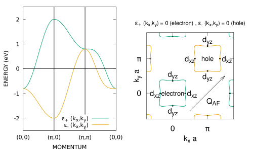
Figure 1: Band structure with perfectly nested Fermi surfaces at half filling, $\varepsilon_{+}({\bi k})=0$ and $\varepsilon_{-}({\bi k})=0$, with hopping matrix elements $t_{1}^{\parallel}=200$ meV, $t_{1}^{\perp}=500$ meV, $t_{2}^{\parallel}=0$, and $t_{2}^{\perp}=100\,i$ meV. Point nodes of quasi-particle gap are marked on Fermi surfaces.

We shall now demonstrate how the perfectly nested Fermi surfaces shown by Fig. 1 can result in an instability to long-range hidden Néel order. It is useful to first write the creation operators for the eigenstates (4) of the electron hopping Hamiltonian, $H_{\rm hop}$:

$$c_{s}^{\dagger}(n,{\bi k})={\cal N}^{-1/2}\sum_{i}\sum_{\alpha=0,1}(-1)^{\alpha n}e^{i(2\alpha-1)\delta(\bi k)}e^{i{\bi k}\cdot{\bi r}_{i}}c_{i,\alpha,s}^{\dagger},$$ (5fh)

where $\alpha=0$ and $1$ index the $d-$ and $d+$ orbitals, and where $n=1$ and $2$ index the anti-bonding and bonding orbitals $(-i)d_{y(\delta)z}$ and $d_{x(\delta)z}$. The inverse of the above is then

$$c_{i,\alpha,s}^{\dagger}={\cal N}^{-1/2}\sum_{\bi k}\sum_{n=1,2}(-1)^{\alpha n}e^{-i(2\alpha-1)\delta({\bi k})}e^{-i{\bi k}\cdot{\bi r}_{i}}c_{s}^{\dagger}(n,{\bi k}).$$ (5fi)

It is then straight-forward to show that the spin magnetization for true ($m=0$) or for hidden ($m=1$) magnetic order,

$$S_{z}(m,{\bi Q}_{\rm AF})=\sum_{i}\sum_{\alpha}(-1)^{\alpha m}e^{i{\bi Q}_{\rm AF}\cdot{\bi r}_{i}}{1\over 2}(n_{i,\alpha,\uparrow}-n_{i,\alpha,\downarrow}),$$ (5fj)

takes the form

$$S_{z}(m,{\bi Q}_{\rm AF})={1\over 2}\sum_{s}\sum_{\bi k}\sum_{n,n^{\prime}}({\rm sgn}\,s){\cal M}_{n,{\bi k};n^{\prime},{\bar{\bi k}}}c_{s}^{\dagger}(n^{\prime},{\bar{\bi k}})c_{s}(n,{\bi k}),$$

(5fk)

where ${\bar{\bi k}}={\bi k}+{\bi Q}_{\rm AF}$. The above matrix element is computed in B. Importantly, it is given by

$${\cal M}_{n,{\bi k};n^{\prime},{\bar{\bi k}}}=\cases{\pm\sin 2\delta({\bi k})&for $n^{\prime}=n+m\;({\rm mod}\;2)$,\\ \pm i\cos 2\delta({\bi k})&for $n^{\prime}=n+m+1\;({\rm mod}\;2)$.}$$ (5fl)

The contribution to the static spin susceptibility from inter-band scattering that corresponds to true ($m=0$) or to hidden ($m=1$) Néel order is then given by the Lindhard function

$$\chi_{\rm inter}(m,{\bi Q}_{\rm AF})=-{1\over{a^{2}N_{\rm Fe}}}\sum_{\bi k}{n_{F}[\varepsilon_{-}({\bar{\bi k}})]-n_{F}[\varepsilon_{+}({\bi k})]\over{\varepsilon_{-}({\bar{\bi k}})-\varepsilon_{+}({\bi k})}}|{\cal M}_{+,{\bi k};-,{\bar{\bi k}}}|^{2},$$ (5fm)

where $n_{\rm F}$ is the Fermi-Dirac distribution.

Next, application of the perfect-nesting condition (5fg) yields a more compact expression for the inter-band contribution to the static spin susceptibility (5fm):

$$\chi_{\rm inter}(m,{\bi Q}_{\rm AF})={1\over{a^{2}N_{\rm Fe}}}\sum_{\bi k}{{1\over 2}-n_{F}[\varepsilon_{+}({\bi k})]\over{\varepsilon_{+}({\bi k})}}|{\cal M}_{+,{\bi k};-,{\bar{\bi k}}}|^{2}.$$ (5fn)

We conclude that the static susceptibilities for true and for hidden Néel order diverge logarithmically as $\chi_{\rm inter}(0,{\bi Q}_{\rm AF})={\rm lim}_{\epsilon\rightarrow 0}\,c^{2}D_{+}(0)\,{\rm ln}(W_{\rm bottom}/\epsilon)$ and $\chi_{\rm inter}(1,{\bi Q}_{\rm AF})={\rm lim}_{\epsilon\rightarrow 0}\,s^{2}D_{+}(0)\,{\rm ln}(W_{\rm bottom}/\epsilon)$, with corresponding density of states weighted by the magnitude square of the matrix element (5fl):

$$c^{2}D_{+}(\varepsilon) = (2\pi)^{-2}\int_{\rm BZ}d^{2}k\,[\cos 2\delta({\bi k})]^{2}\delta[\varepsilon-\varepsilon_{+}({\bi k})],$$ (5fo)

$$s^{2}D_{+}(\varepsilon) = (2\pi)^{-2}\int_{\rm BZ}d^{2}k\,[\sin 2\delta({\bi k})]^{2}\delta[\varepsilon-\varepsilon_{+}({\bi k})].$$ (5fp)

Above, $W_{\rm bottom}=-\varepsilon_{+}(0,0)$. The weighted densities of states (5fo) and (5fp) are of comparable strength at the Fermi level, $\varepsilon=0$. For example, numerical calculations that are described in the caption to Fig. 2 yield the values $c^{2}D_{+}(0)=0.135\,a^{-2}{\rm eV}^{-1}$ and $s^{2}D_{+}(0)=0.072\,a^{-2}{\rm eV}^{-1}$ for these quantities. Here, hopping matrix elements coincide with those listed in the caption to Fig. 1. Hidden magnetic order is therefore possible.

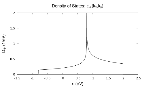
Figure 2: Density of states of the bonding band evaluated numerically at hopping parameters that are listed in the caption to Fig. 1: $a^{2}D_{+}(\varepsilon)=N_{\rm Fe}^{-1}\sum_{\bi k}\delta[\varepsilon-\varepsilon_{+}({\bi k})]$. The one-iron Brillouin zone is divided into a $10,000\times 10,000$ grid, while the $\delta$-function is approximated by $(4k_{B}T_{0})^{-1}{\rm sech}^{2}(\varepsilon/2k_{B}T_{0})$. Here, $k_{B}T_{0}$ is $3$ parts in $10,000$ of the bandwidth. The peak is a logarithmic van Hove singularity at $\varepsilon_{+}(\pi/a,\pi/a)$.

3 Hidden magnetic order and excitations

We have just seen how the perfect nesting of the Fermi surfaces shown by Fig. 1 results in an instability towards long-range Néel order per $d+$ and $d-$ orbital. Below, we shall introduce an extended Hubbard model over the square lattice that includes these orbitals alone. Within mean field theory, we shall see that long-range hidden Néel order exists at half filling because of magnetic frustration by super-exchange interactions[24, 25].

3.1 Extended Hubbard model

We shall now add on-site interactions due to Coulomb repulsion and super-exchange interactions via the Se atoms to the hopping Hamiltonian (1). The Hamiltonian then has three parts: $H=H_{\rm hop}+H_{U}+H_{\rm sprx}$. On-site Coulomb repulsion is counted by the second term[38],

$$H_{U}=\sum_{i} [U_{0}n_{i,\alpha,\uparrow}n_{i,\alpha,\downarrow}+J_{0}{\bi S}_{i,d-}\cdot{\bi S}_{i,d+}$$ (5fq)

$$+U_{0}^{\prime}n_{i,d+}n_{i,d-}+J_{0}^{\prime}(c_{i,d+,\uparrow}^{\dagger}c_{i,d+,\downarrow}^{\dagger}c_{i,d-,\downarrow}c_{i,d-,\uparrow}+{\rm h.c.})],$$

where $n_{i,\alpha,s}=c_{i,\alpha,s}^{\dagger}c_{i,\alpha,s}$ is the occupation operator, where ${\bi S}_{i,\alpha}=\sum_{s,s^{\prime}}c_{i,\alpha,s}^{\dagger}{\boldsymbol{\sigma}}_{s,s^{\prime}}c_{i,\alpha,s^{\prime}}$ is the spin operator, and where $n_{i,\alpha}=n_{i,\alpha,\uparrow}+n_{i,\alpha,\downarrow}$. Above, $U_{0}>0$ denotes the intra-orbital on-site Coulomb repulsion energy, while $U_{0}^{\prime}>0$ denotes the inter-orbital one. Also, $J_{0}<0$ is the Hund’s Rule exchange coupling constant, which is ferromagnetic, while $J_{0}^{\prime}$ denotes the matrix element for on-site-orbital Josephson tunneling.

The third and last term in the Hamiltonian represents super-exchange interactions among the iron spins via the selenium atoms:

$$H_{\rm sprx}=\sum_{\langle i,j\rangle} J_{1}^{({\rm sprx})}({\bi S}_{i,d-}+{\bi S}_{i,d+})\cdot({\bi S}_{j,d-}+{\bi S}_{j,d+})$$ (5fr)

$$+\sum_{\langle\langle i,j\rangle\rangle}J_{2}^{({\rm sprx})}({\bi S}_{i,d-}+{\bi S}_{i,d+})\cdot({\bi S}_{j,d-}+{\bi S}_{j,d+}).$$

Above, $J_{1}^{({\rm sprx})}$ and $J_{2}^{({\rm sprx})}$ are positive super-exchange coupling constants over nearest neighbor and next-nearest neighbor iron sites. We shall assume henceforth that magnetic frustration is moderate to strong: $J_{2}^{({\rm sprx})}>0.5J_{1}^{({\rm sprx})}$. In isolation, the above term of the Hamiltonian then favors “stripe” spin-density wave order at half filling over conventional Néel order.

3.2 Mean field theory

Following the mean-field treatment of antiferromagnetism in the conventional Hubbard model over the square lattice at half filling[27, 28, 29, 30], assume that the expectation value of the magnetic moment per site, per orbital, shows hidden Néel order:

$$\langle m_{i,\alpha}\rangle=(-1)^{\alpha}e^{i{\bi Q}_{\rm AF}\cdot{\bi r}_{i}}\langle m_{0,0}\rangle,$$ (5fs)

where $\langle m_{i,\alpha}\rangle={1\over 2}\langle n_{i,\alpha,\uparrow}\rangle-{1\over 2}\langle n_{i,\alpha,\downarrow}\rangle$. Previous calculations in the local-moment limit (5faobgbo) indicate that the above hidden magnetic order is more stable than the “stripe” spin-density wave (SDW) mentioned above at weak to moderate strength in the Hund’s Rule coupling[18, 25]. The super-exchange terms, $H_{\rm sprx}$, make no contribution within the mean-field approximation, since the net magnetic moment per iron atom is null in the hidden-order Néel state. And we shall neglect the on-site Josephson tunneling term in (5fq) $H_{U}$. This is valid at the strong-coupling limit, $U_{0}\rightarrow\infty$, where the formation of a spin singlet per iron-site-orbital is suppressed. We are then left with the two on-iron–site repulsion terms and the Hund’s Rule term in $H_{U}$.

The mean-field replacement of the intra-orbital on-site term ($U_{0}$) is the standard one[27]. In particular, replace

$$n_{i,\alpha,\uparrow}n_{i,\alpha,\downarrow}\rightarrow{1\over 2}\langle n_{i,\alpha}\rangle(n_{i,\alpha,\uparrow}+n_{i,\alpha,\downarrow}) -\langle m_{i,\alpha}\rangle(n_{i,\alpha,\uparrow}-n_{i,\alpha,\downarrow})$$

$$-\langle n_{i,\alpha,\uparrow}\rangle\langle n_{i,\alpha,\downarrow}\rangle.$$

The first term above can be absorbed into the chemical potential because $\langle n_{i,d-}\rangle=\langle n_{i,d+}\rangle$, the last term above is a constant energy shift, leaving a mean-field contribution to the Hamiltonian $-\sum_{i}\sum_{\alpha}U_{0}\langle m_{i,\alpha}\rangle(n_{i,\alpha,\uparrow}-n_{i,\alpha,\downarrow})$. The mean-field replacement of the inter-orbital on-iron-site repulsion term ($U_{0}^{\prime}$) in $H_{U}$ is also standard:

$$n_{i,d+}n_{i,d-}\rightarrow n_{i,d+}\langle n_{i,d-}\rangle+\langle n_{i,d+}\rangle n_{i,d-}-\langle n_{i,d+}\rangle\langle n_{i,d-}\rangle.$$

The first two terms above can again be absorbed into a shift of the chemical potential, while the third and last term above is again a constant energy shift. The inter-orbital repulsion term, hence, makes no contribution to the Hamiltonian within the mean-field approximation. Last, we make the same type of mean-field replacement for the Hund’s Rule term ($J_{0}$) in $H_{U}$:

$${\bi S}_{i,d+}\cdot{\bi S}_{i,d-}\rightarrow S_{i,d+}^{(z)}\langle S_{i,d-}^{(z)}\rangle+\langle S_{i,d+}^{(z)}\rangle S_{i,d-}^{(z)}-\langle S_{i,d+}^{(z)}\rangle\langle S_{i,d-}^{(z)}\rangle.$$

Again, the last term above is just a constant energy shift. The first two terms, however, contribute to the mean-field Hamiltonian: $\sum_{i}\sum_{\alpha}{1\over 2}J_{0}\langle m_{i,{\bar{\alpha}}}\rangle(n_{i,\alpha,\uparrow}-n_{i,\alpha,\downarrow})$, which is equal to $-\sum_{i}\sum_{\alpha}{1\over 2}J_{0}\langle m_{i,\alpha}\rangle(n_{i,\alpha,\uparrow}-n_{i,\alpha,\downarrow})$ in the case of hidden magnetic order (5fs). Here, $\overline{d\pm}=d\mp$.

The net contribution to the mean-field Hamiltonian from interactions in the present two-orbital Hubbard model is then

$$-\sum_{i}\sum_{\alpha}U(\pi)\langle m_{i,\alpha}\rangle(n_{i,\alpha,\uparrow}-n_{i,\alpha,\downarrow})=-\langle m_{0,0}\rangle U(\pi)\sum_{i}\sum_{\alpha}(-1)^{\alpha}e^{i{\bi Q}_{\rm AF}\cdot{\bi r}_{i}}(n_{i,\alpha,\uparrow}-n_{i,\alpha,\downarrow}),$$

where

$$U(\pi)=U_{0}+{1\over 2}J_{0}.$$ (5ft)

Notice that the last sum above is simply twice the hidden ($m=1$) ordered moment $S_{z}(m,{\bi Q}_{\rm AF})$ defined by (5fj). Inspection of (5fk) then yields that the mean-field Hamiltonian for the present two-orbital Hubbard model takes the form

$$H^{(mf)}= \sum_{s}\sum_{\bi k}\sum_{n}\varepsilon_{n}({\bi k})c_{s}^{\dagger}(n,{\bi k})c_{s}(n,{\bi k})$$ (5fu)

$$\mp\sum_{s}\sum_{\bi k}[({\rm sgn}\,s)\Delta({\bi k})c_{s}^{\dagger}(1,{\bar{\bi k}})c_{s}(2,{\bi k})+{\rm h.c.}],$$

with a gap function

$$\Delta({\bi k})=\Delta_{0}\sin[2\delta({\bi k})],$$ (5fv)

where ${\bar{\bi k}}={\bi k}+{\bi Q}_{\rm AF}$, and where

$$\Delta_{0}=\langle m_{0,0}\rangle U(\pi).$$ (5fw)

Here, we have used the result (5fl) for the matrix element in the case of hidden magnetic order ($m=1$). Here also, intra-band scattering ($n^{\prime}=n$) has been neglected because it shows no nesting. After shifting the sum in momentum of the first term in (5fu) by ${\bi Q}_{AF}$ for the anti-bonding band, $n=1$, we arrive at the final form of the mean-field Hamiltonian:

$$H^{(mf)}= \sum_{s}\sum_{\bi k}\varepsilon_{+}({\bi k})[c_{s}^{\dagger}(2,{\bi k})c_{s}(2,{\bi k})-c_{s}^{\dagger}(1,{\bar{\bi k}})c_{s}(1,{\bar{\bi k}})]$$ (5fx)

$$+\sum_{s}\sum_{\bi k}[({\rm sgn}\,s)\Delta({\bi k})c_{s}^{\dagger}(1,{\bar{\bi k}})c_{s}(2,{\bi k})+{\rm h.c.}].$$

Above, we have set the $\pm$ sign in the matrix element (5fl) to minus for convenience.

The mean-field Hamiltonian (5fx) is diagonalized in the standard way by writing the electron in terms of new quasi-particle excitations[28, 29, 30]:

$$c_{s}^{\dagger}(2,{\bi k}) = u({\bi k})\alpha_{s}^{\dagger}(2,{\bi k})-({\rm sgn}\,s)v({\bi k})\alpha_{s}^{\dagger}(1,{\bar{\bi k}}),$$

$$c_{s}^{\dagger}(1,{\bar{\bi k}}) = ({\rm sgn}\,s)v({\bi k})\alpha_{s}^{\dagger}(2,{\bi k})+u({\bi k})\alpha_{s}^{\dagger}(1,{\bar{\bi k}}).$$ (5fy)

Above, $u({\bi k})$ and $v({\bi k})$ are coherence factors with square magnitudes

$$u^{2}={1\over 2}+{1\over 2}{\varepsilon_{+}\over E}\quad{\rm and}\quad v^{2}={1\over 2}-{1\over 2}{\varepsilon_{+}\over E},$$ (5fz)

where $E({\bi k})=[\varepsilon_{+}^{2}({\bi k})+\Delta^{2}({\bi k})]^{1/2}$. The mean-field Hamiltonian can then be expressed in terms of the occupation of quasiparticles by

$$H^{(mf)}=\sum_{s}\sum_{\bi k}E({\bi k})[\alpha_{s}^{\dagger}(2,{\bi k})\alpha_{s}(2,{\bi k})-\alpha_{s}^{\dagger}(1,{\bar{\bi k}})\alpha_{s}(1,{\bar{\bi k}})].$$ (5faa)

The quasi-particle excitation energies are then $E({\bi k})$ for particles and $E({\bar{\bi k}})$ for holes. Notice that the gap (5fv) in the excitation spectrum has $D_{xy}$ symmetry. (See Fig. 1.) At half filling then, the energy band $-E({\bar{\bi k}})$ is filled, while the energy band $+E({\bi k})$ is empty. Last, inverting (5fy) yields

$$\alpha_{s}^{\dagger}(2,{\bi k}) = u({\bi k})c_{s}^{\dagger}(2,{\bi k})+({\rm sgn}\,s)v({\bi k})c_{s}^{\dagger}(1,{\bar{\bi k}}),$$

$$\alpha_{s}^{\dagger}(1,{\bar{\bi k}}) = -({\rm sgn}\,s)v({\bi k})c_{s}^{\dagger}(2,{\bi k})+u({\bi k})c_{s}^{\dagger}(1,{\bar{\bi k}}).$$ (5fab)

As expected, the quasiparticles are a coherent superposition of an electron of momentum ${\bi k}$ in the bonding band $2$ with an electron of momentum ${\bi k}+{\bi Q}_{\rm AF}$ in the anti-bonding band $1$.

Finally, to obtain the gap equation, we exploit the pattern of hidden Néel order (5fs), and equivalently write the gap maximum (5fw) as

$$\Delta_{0}={\cal N}^{-1}\sum_{i}\sum_{\alpha}U(\pi)\langle m_{i,\alpha}\rangle(-1)^{\alpha}e^{i{\bi Q}_{\rm AF}\cdot{\bi r}_{i}}={\cal N}^{-1}U(\pi)\langle S_{z}(1,{\bi Q}_{\rm AF})\rangle.$$

Using expression (5fk) and the result (5fl) in the case of hidden magnetic order ($m=1$) yields the relationship

$$\Delta_{0}=-{\cal N}^{-1}{1\over 2}\sum_{s}\sum_{\bi k}\sum_{n}U(\pi)({\rm sgn}\,s)[\sin\,2\delta({\bi k})]\langle c_{s}^{\dagger}({\bar{n}},{\bar{\bi k}})c_{s}(n,{\bi k})\rangle,$$

where ${\bar{n}}=1+(n\;{\rm mod}\;2)$. Again, we have neglected intra-band scattering. Also, notice that the sums over the bands (4) and the spins yield the hSDW order parameter

$$i\langle c_{s}^{\dagger}(d_{y({\bar{\delta}})z},{\bar{\bi k}})c_{s}(d_{x(\delta)z},{\bi k})-c_{s}^{\dagger}(d_{x({\bar{\delta}})z},{\bar{\bi k}})c_{s}(d_{y(\delta)z},{\bi k})\rangle({\rm sgn}\,s),$$ (5fac)

which is orbitally isotropic. Substituting in (5fy) and the conjugate annihilation operators, and recalling that the $n=1$ quasi-particle band is filled in the groundstate, while the $n=2$ quasi-particle band is empty, yields $\langle c_{s}^{\dagger}({\bar{n}},{\bar{\bi k}})c_{s}(n,{\bi k})\rangle=-({\rm sgn}\,s)u({\bi k})v({\bi k})$ for the expectation value. We thereby obtain the relationship

$$\Delta_{0}={\cal N}^{-1}\sum_{\bi k}U(\pi)[\sin\,2\delta({\bi k})]\Delta({\bi k})/E({\bi k}),$$

or equivalently, the gap equation

$$1=U(\pi){\cal N}^{-1}\sum_{\bi k}{[\sin\,2\delta({\bi k})]^{2}\over{\sqrt{\varepsilon_{+}^{2}({\bi k})+\Delta_{0}^{2}[\sin\,2\delta({\bi k})]^{2}}}}.$$ (5fad)

In the limit $\Delta_{0}\rightarrow\infty$, we then have $\Delta_{0}=U(\pi){\cal N}^{-1}\sum_{\bi k}|\sin\,2\delta({\bi k})|$, which yields a hidden-order moment $\langle m_{0,0}\rangle={\cal N}^{-1}\sum_{\bi k}|\sin\,2\delta({\bi k})|$ bounded by $1/2$. In the special case $|t_{1}^{\perp}|=2|t_{2}^{\perp}|$, inspection of (5fb) yields $|\sin\,2\delta({\bi k})|=|\sin\,k_{x}a||\sin\,k_{y}a|/[1-(\cos\,k_{x}a)(\cos\,k_{y}a)]$. In the thermodynamic limit, $N_{\rm Fe}\rightarrow\infty$, integration along one of the principal axes followed by a series expansion in turn yields $\langle m_{0,0}\rangle=1/4$ for the previous expression. In the limit $|t_{1}^{\perp}|\rightarrow 0$, on the other hand, we have $|\sin\,2\delta({\bi k})|\rightarrow 1$ by (5fb), which yields an ordered magnetic moment $\langle m_{0,0}\rangle=1/2$. Figure 3 shows the ordered magnetic moment at $U_{0}\rightarrow\infty$ versus hybridization of the $3d_{xz}$ and $3d_{yz}$ orbitals.

The above mean field theory predicts quasiparticles with excitation energies that disperse as $E_{+}({\bi k})$ and $E_{-}({\bi k})$, where $E_{\pm}({\bi k})=(\varepsilon_{\pm}^{2}({\bi k})+\Delta_{0}^{2}[\sin 2\delta({\bi k})]^{2})^{1/2}$. They reach zero at point nodes located where the Fermi surface crosses a principal axis, at which the phase shift $\delta({\bi k})$ is a multiple of $\pi/2$. These point nodes are shown by Fig. 1. The quasi-particle energy spectra disperse about the nodes in a Dirac-cone fashion: $E({\bi k})\cong[v_{F}^{2}k_{\perp}^{2}+(2\Delta_{0}\delta_{D}^{\prime})^{2}k_{\parallel}^{2}]^{1/2}$, where $v_{F}$ is the Fermi velocity of $\varepsilon_{\pm}({\bi k})$ at the node, and where $\delta_{D}^{\prime}$ is the gradient of the phase shift $\delta({\bi k})$ at the node. Here $(k_{\parallel},k_{\perp})$ denote the momentum coordinates about a point node in the directions parallel and perpendicular to the Fermi surface there. Last, notice that combining the spectra $E_{+}({\bi k})$ and $E_{-}({\bi k})$ in the folded Brillouin zone results in four Dirac cones at the Fermi level. (C.f. ref. [39]).

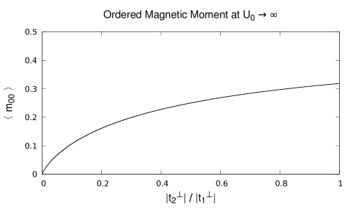
Figure 3: Shown is the ordered magnetic moment at $U_{0}\rightarrow\infty$: $\langle m_{0,0}\rangle=(2N_{\rm Fe})^{-1}\sum_{\bi k}|\sin\,2\delta({\bi k})|$. The one-iron Brillouin zone is divided into a $10,000\times 10,000$ grid.

3.3 Low-energy collective modes

The groundstate of the above mean field theory is the filled energy band $-E({\bar{\bi k}})$: $|\Psi_{0}\rangle=\prod_{{\bi k},s}\alpha_{s}^{\dagger}(1,{\bi k})|0\rangle$. Inspection of (5fab) yields that it can also be expressed as

$$|\Psi_{0}\rangle=\prod_{{\bi k},s}[u({\bar{\bi k}})-({\rm sgn}\,s)v({\bar{\bi k}})c_{s}^{\dagger}(2,{\bar{\bi k}})c_{s}(1,{\bi k})]|1\rangle,$$ (5fae)

where $|1\rangle=\prod_{{\bi k},s}c_{s}^{\dagger}(1,{\bi k})|0\rangle$ is the filled anti-bonding band of non-interacting electrons. Next, observe that each pair of factors above per momentum over spin $\uparrow$ and $\downarrow$ can be expressed as $u^{2}({\bar{\bi k}})\,{\rm exp}(-[v({\bar{\bi k}})/u({\bar{\bi k}})]{\hat{\bi n}}\cdot\sum_{s_{1},s_{2}}c_{s_{1}}^{\dagger}(2,{\bar{\bi k}}){\boldsymbol{\sigma}}_{s_{1},s_{2}}c_{s_{2}}(1,{\bi k}))$, with unit vector ${\hat{\bi n}}$ along with the $z$ axis. Now define a new spin quantization axis $z^{\prime}=y$, along with the remaining axes $x^{\prime}=z$ and $y^{\prime}=x$. If, more generally, we let the axis of the sub-lattice magnetization ${\hat{\bi n}}$ lie in the $z$-$x$ plane, then the spin operator in the argument of the exponential above becomes

$$\sum_{s_{1},s_{2}}c_{s_{1}}^{\prime\,\dagger}(2,{\bar{\bi k}})[(\cos\,\phi)\sigma_{x}+(\sin\,\phi)\sigma_{y}]_{s_{1},s_{2}}c_{s_{2}}^{\prime}(1,{\bi k}).$$

Here, $c_{s}^{\prime}$ and $c_{s}^{\prime\,\dagger}$ are the electron annihilation and creation operators in the new quantization axes. Here also, $\phi$ is the angle that ${\hat{\bi n}}$ makes with the $z$ axis. Re-expanding the exponential operator above then yields the groundstate (5fae) in the new quantization axes:

$$|\Psi_{0}(\phi)\rangle=\prod_{{\bi k}} [u({\bar{\bi k}})-e^{-i\phi}v({\bar{\bi k}})c_{\uparrow}^{\prime\,\dagger}(2,{\bar{\bi k}})c_{\downarrow}^{\prime}(1,{\bi k})]$$ (5faf)

$$\cdot[u({\bar{\bi k}})-e^{+i\phi}v({\bar{\bi k}})c_{\downarrow}^{\prime\,\dagger}(2,{\bar{\bi k}})c_{\uparrow}^{\prime}(1,{\bi k})]|1\rangle.$$

It has indefinite spin $S_{y}$ along the new quantization axis:

$$|\Psi_{0}(\phi)\rangle=\sum_{m=-N_{\rm Fe}}^{N_{\rm Fe}}e^{-im\phi}|\Psi_{0}^{(m)}\rangle,$$ (5fag)

where $|\Psi_{0}^{(m)}\rangle$ are projections of the groundstate that have spin $S_{y}$ equal to $m\hbar$. Then because $S_{y}=i\hbar{\partial\over{\partial\phi}}$, we have that the macroscopic phase angle and the macroscopic spin along the $y$ axis satisfy the commutation relationship[40] $[\phi,S_{y}]=-i\hbar$.

Define, next, the macroscopic magnetization, $M_{y}=S_{y}/V$, where $V$ is the area, and let it and the phase angle $\phi$ vary slowly over the bulk. Their dynamics is then governed by the hydrodynamic Hamiltonian[41, 42] $H_{\rm hydro}=\int d^{2}r\,{\cal H}_{\rm hydro}$, with the Hamiltonian density

$${\cal H}_{\rm hydro}={1\over{2\chi_{\perp}}}M_{y}^{2}+{1\over 2}\rho_{s}|{\bi\nabla}\phi|^{2}.$$ (5fah)

Above, $\chi_{\perp}$ and $\rho_{s}$ denote, respectively, the transverse spin susceptibility and the spin stiffness of the present hidden spin-density wave state. Given the commutation relationship $[\phi({\bi r}),M_{y}({\bi r}^{\prime})]=-i\hbar\,\delta^{(2)}({\bi r}-{\bi r}^{\prime})$, we obtain the following dynamical equations:

$${\dot{M}_{y}} = -\rho_{s}\nabla^{2}\phi,$$

$${\dot{\phi}} = -M_{y}/\chi_{\perp}.$$ (5fai)

The magnetization thus satisfies the wave equation ${\ddot{M}_{y}}=c_{0}^{2}\nabla^{2}M_{y}$, with propagation velocity $c_{0}=(\rho_{s}/\chi_{\perp})^{1/2}$. We conclude that the present hidden spin-density wave state supports antiferromagnetic spin-wave excitations that disperse acoustically in frequency: $\omega({\bar{\bi k}})=c_{0}|{\bi k}|$. And since the above dynamics can be rotated by $90$ degrees about the $z$ axis, there then exist two acoustic spin-wave excitations per momentum.

3.4 Transverse spin susceptibility and spin rigidity

To compute the transverse spin susceptibility, we apply an external magnetic field along the $y$ axis by adding the term $-h\sum_{i}\sum_{\alpha}S_{i,\alpha}^{(y)}$ to the Hamiltonian $H_{\rm hop}+H_{U}+ H_{\rm sprx}$. The on-site-orbital repulsion terms, the Hund’s Rule coupling terms, and the super-exchange terms can then be replaced by the isotropic mean-field approximations

$$n_{i,\alpha,\uparrow}n_{i,\alpha,\downarrow}\rightarrow{1\over 2}\langle n_{i,\alpha}\rangle(n_{i,\alpha,\uparrow}+n_{i,\alpha,\downarrow}) -2\langle{\bi m}_{i,\alpha}\rangle\cdot{\bi S}_{i,\alpha}$$

$$-\langle n_{i,\alpha,\uparrow}\rangle\langle n_{i,\alpha,\downarrow}\rangle$$

and

$${\bi S}_{i,\alpha}\cdot{\bi S}_{j,\beta}\rightarrow{\bi S}_{i,\alpha}\cdot\langle{\bi S}_{j,\beta}\rangle+\langle{\bi S}_{i,\alpha}\rangle\cdot{\bi S}_{j,\beta}-\langle{\bi S}_{i,\alpha}\rangle\cdot\langle{\bi S}_{j,\beta}\rangle.$$

Yet the external magnetic field cants the antiferromagnetically aligned moments per orbital along the $y$ axis by the transverse magnetization per orbital, $\langle m_{\perp}\rangle$. It makes a contribution to the above mean-field replacements that can be accounted for by making the replacement $h\rightarrow h+2U(0)\langle m_{\perp}\rangle$ in the paramagnetic term that we added above to the Hamiltonian, where

$$U(0)=U_{0}-{1\over 2}J_{0}-4J_{1}^{({\rm sprx})}-4J_{2}^{({\rm sprx})}.$$ (5faj)

We thereby arrive at the formula

$$\chi_{\perp}={\chi_{\perp}^{(0)}\over{1-a^{2}U(0)\chi_{\perp}^{(0)}}}$$ (5fak)

for the transverse spin susceptibility per iron atom, where $\chi_{\perp}^{(0)}$ is the naive transverse spin susceptibility that neglects the effect of canting.

The formula for the naive transverse spin susceptibility is well known[43], and it is derived in C. It reads

$$\chi_{\perp}^{(0)}={1\over 2}(a^{2}N_{\rm Fe})^{-1}\sum_{\bi k}{\Delta^{2}({\bi k})\over{[\varepsilon_{+}^{2}({\bi k})+\Delta^{2}({\bi k})]^{3/2}}}.$$ (5fal)

At the weak-coupling limit, $U(0),U(\pi)\rightarrow 0$, the transverse spin susceptibility (5fak) is given by $\chi_{\perp}^{(0)}$, and the quotient in the sum over momentum above is equal to $2\,\delta[\varepsilon_{+}({\bi k})]$. We thereby obtain the Pauli paramagnetic susceptibility at weak-coupling,

$${\rm lim}_{U(0),U(\pi)\rightarrow 0}\chi_{\perp}=D_{+}(0),$$ (5fam)

where $D_{+}(\varepsilon)$ is the density of states of the bonding band $\varepsilon_{+}({\bi k})$. (See Fig. 2.)

At the strong-coupling limit, $U_{0}\rightarrow\infty$, it’s useful to re-write the formula (5fak) as[43]

$$\chi_{\perp}={1\over{a^{2}U(0)}}\Biggl{[}{1\over{1-a^{2}U(0)\chi_{\perp}^{(0)}}}-1\Biggr{]}.$$ (5fan)

Observe, next, the following identity for the quotient in (5fal):

$${\Delta^{2}({\bi k})\over{E^{3}({\bi k})}}={[\sin\,2\delta({\bi k})]^{2}\over{E({\bi k})}}+{[\cos\,2\delta({\bi k})]^{2}\over{E({\bi k})}}-{\varepsilon_{+}^{2}(\bi k)\over{E^{3}({\bi k})}}.$$

Applying the gap equation (5fad) then yields the result $a^{2}U(\pi)\chi_{\perp}^{(0)}=1+I_{1}-I_{2}$, where

$$I_{1} = {1\over 2}N_{\rm Fe}^{-1}\sum_{\bi k}{[\cos 2\delta({\bi k})]^{2}\over{E({\bi k})}}U(\pi),$$ (5faoa)

$$I_{2} = {1\over 2}N_{\rm Fe}^{-1}\sum_{\bi k}{\varepsilon_{+}^{2}{\bi k})\over{E^{3}({\bi k})}}U(\pi).$$ (5faob)

In the limit $U_{0}\rightarrow\infty$, it can be shown that $I_{1}=I_{2}$ as the pure-imaginary hopping matrix element $t_{2}^{\perp}$ tends to zero. (See C.) In such case, $a^{2}U(\pi)\chi_{\perp}^{(0)}=1$, and we thereby achieve the result

$${\rm lim}_{U_{0}\rightarrow\infty}\chi_{\perp} = {1\over{a^{2}U(0)}}\Biggl{(}\Biggl{[}1-{U(0)\over{U(\pi)}}\Biggr{]}^{-1}-1\Biggr{)}$$ (5faoap)

$$= a^{-2}[J_{0}+4J_{1}^{({\rm sprx})}+4J_{2}^{({\rm sprx})}]^{-1}.$$

It coincides precisely with the corresponding result for the Heisenberg model (5faobgbo) [25] after making the assignments $J_{1}^{\parallel}=J_{1}^{({\rm sprx})}$ and $J_{2}^{\perp}=J_{2}^{({\rm sprx})}$ for two of the exchange coupling constants. Here $J_{n}^{\parallel}$ and $J_{n}^{\perp}$ represent intra-orbital and inter-orbital Heisenberg exchange coupling constants among the $d+$ and $d-$ orbitals.

Next, to compute the spin stiffness $\rho_{s}$ at half filling, we follow the calculation of the same quantity in the case of the conventional Hubbard model over the square lattice[28, 29, 30, 43, 44]. At zero temperature, the spin rigidity saturates the f-sum rule for the spin current. We therefore arrive at the expression

$$\rho_{s}={1\over{N_{\rm Fe}}}\sum_{\bi k}[u^{2}({\bi k})-v^{2}({\bi k})]{1\over 4}\varepsilon_{\parallel}({\bi k})$$ (5faoaq)

for it. Here, we have taken the average over the two principal axes. In the weak-coupling limit, where the gap function vanishes, we therefore get ${\rm lim}_{U(\pi)\rightarrow 0}\,\rho_{s}=N_{\rm Fe}^{-1}\sum_{\bi k}^{\prime}t_{1}^{\parallel}(\cos\,k_{x}a+\cos\,k_{y}a)$, where the prime notation indicates the condition that $\varepsilon_{+}({\bi k})<0$. In such case, the sum over momenta lies inside the Fermi surface at the center of the Brillouin zone. (See Fig. 1.) At strong coupling $U(\pi)\rightarrow\infty$, on the other hand, it is useful to return to the original expression (5faoaq):

$$\rho_{s}={1\over{N_{\rm Fe}}}\sum_{\bi k}{1\over 4}{\varepsilon_{+}({\bi k})\cdot\varepsilon_{\parallel}({\bi k})\over{\sqrt{\varepsilon_{+}^{2}({\bi k})+\Delta_{0}^{2}[\sin\,2\delta({\bi k})]^{2}}}}.$$ (5faoar)

Here, we have substituted in the expressions for the coherence factors (5fz). Approximate now all dispersions in energy about the Dirac nodes at the Fermi surface $\varepsilon_{+}({\bi k})=0$: e.g.; $\varepsilon_{+}({\bi k})\cong v_{F}(k_{x}-k_{D})$, $\varepsilon_{\parallel}({\bi k})\cong\varepsilon_{\parallel}(k_{D},0)+v_{\parallel}(k_{x}-k_{D})$, and $\sin\,2\delta({\bi k})\cong 2\delta_{D}^{\prime}k_{y}$, where the coordinates of the Dirac node are $(k_{D},0)$. After taking the thermodynamic limit, $N_{\rm Fe}\rightarrow\infty$, and after cutting off the resulting integrals in momentum by $k_{1}\sim k_{D}/2$ in both the $x$ and in the $y$ directions, we obtain the following result in the limit of strong coupling:

$${\rm lim}_{U(\pi)\rightarrow\infty}\,\rho_{s}={2\over 3}{(k_{1}a)^{3}\over{(2\pi)^{2}}}{v_{\rm F}v_{\parallel}\over{\delta_{D}^{\prime}\Delta_{0}}}{1\over a}{\rm ln}\Bigl{(}2e^{1/3}{2\delta_{D}^{\prime}\Delta_{0}\over{v_{F}}}\Bigr{)}.$$ (5faoas)

In this limit, the spin stiffness at half filling therefore scales as $\rho_{s}\sim(t^{2}/U){\rm ln}(U/t)$ with the scale of the hopping matrix elements $t$, and with the scale of the on-site repulsion energy $U$. It is useful to compare the latter result for the rigidity of hidden magnetic order at strong on-site-orbital repulsion (5faoas) with that obtained from the corresponding two-orbital Heisenberg model (5faobgbo) [25]: $\rho_{s}=2s_{0}^{2}[J_{1}^{\parallel}-J_{1}^{\perp}+2(J_{2}^{\perp}-J_{2}^{\parallel})]$. It yields the assignments $J_{1}^{\perp}=J_{1}^{({\rm sprx})}-\rho_{s}/2s_{0}^{2}$ and $J_{2}^{\parallel}=J_{2}^{({\rm sprx})}$ for the remaining two exchange coupling constants.

4 Eliashberg theory

The previous mean-field approximation of the extended two-orbital Hubbard model for a single layer of heavily electron-doped iron-selenide predicts Dirac quasi-particle excitations at nodes where the Fermi surface crosses a principal axis. (See Fig. 1.) Below, we shall demonstrate how the Fermi surface at weak coupling experiences a Lifshitz transition to Fermi-surface pockets at the corner of the two-iron Brillouin zone as the on-site-orbital repulsion grows strong. We will achieve this by first formulating an Eliashberg theory for the extended Hubbard model in the electron-hole channel.

4.1 Hidden spinwaves and interaction with electrons

It was revealed in section 3.3 that the above mean field theory for the hidden Néel state of the Hubbard model over the square lattice harbors spin-wave excitations that collapse to zero energy at the Néel wavenumber ${\bi Q}_{\rm AF}$. The hidden Néel state of the corresponding Heisenberg model over the square lattice exhibits the very same hidden spin-wave excitations[25]. Consider then the propagator for hidden spinwaves: $iD({\bi q},\omega)=\langle{1\over{\sqrt{2}}}m^{+}(\pi){1\over{\sqrt{2}}}m^{-}(\pi)\rangle|_{{\bi q},\omega}$, where $m^{\pm}(\pi)=m_{x}(\pi)\pm i\,m_{y}(\pi)$. Here, ${\bi m}(\pi)={\bi m}_{d-}-{\bi m}_{d+}$ is the hidden magnetic moment. The propagator takes the form

$$D({\bi q},\omega)={(2s_{1})^{2}\over{\chi_{\perp}}}[\omega^{2}-\omega_{b}^{2}({\bi q})]^{-1}$$ (5faoat)

in the case of the above mean-field theory, as well as in the case of the linear spin-wave approximation of the Heisenberg model (5faobgbo) [25]. It shows a pole in frequency that disperses acoustically as $\omega_{b}({\bar{\bi q}})=c_{0}|{\bi q}|$ about ${\bi Q}_{\rm AF}$, where $c_{0}=(\rho_{s}/\chi_{\perp})^{1/2}$ is the hidden-spin-wave velocity, and where ${\bar{\bi q}}={\bi q}+{\bi Q}_{\rm AF}$. In the former case, $s_{1}$ is equal to the sub-lattice magnetization, $\langle m_{0,0}\rangle$, while $s_{1}$ is given by the electron spin in the latter case. Last, $\chi_{\perp}$ is the transverse spin susceptibility of the hidden Néel state.

The previous mean-field theory implies that the hidden spinwaves in question interact with independent electrons governed by the hopping Hamiltonian, $H_{\rm hop}$. This is evident from the mean-field form of the interaction (5ft) in isotropic form: $-\sum_{i}\sum_{\alpha}U(\pi){\bi m}_{i,\alpha}\cdot 2{\bi S}_{i,\alpha}$. The transverse contributions yield the interaction $-\sum_{i}\sum_{\alpha}U(\pi)(m_{i,\alpha}^{+}S_{i,\alpha}^{-}+m_{i,\alpha}^{-}S_{i,\alpha}^{+}$). Plugging in expression (5fi) and its conjugate for the electron creation and destruction operators yields the following interaction contribution to the Hamiltonian with hidden spinwaves:

$$H_{\rm e-hsw}=-{1\over{\sqrt{2}}}{U(\pi)\over{a{\cal N}^{1/2}}}\sum_{\bi k}\sum_{{\bi k}^{\prime}}\sum_{n}[m^{+}(\pi,{\bi q})c_{\downarrow}^{\dagger}({\bar{n}},{\bar{\bi k}}^{\prime})c_{\uparrow}(n,{\bi k}) {\cal M}_{n,{\bi k};{\bar{n}},{\bar{\bi k}}^{\prime}}$$ (5faoau)

$$+{\rm h.c.}],$$

where ${\bi q}={\bi k}-{\bar{\bi k}}^{\prime}$ is the momentum transfer, and where the matrix element above is the prior one for hidden order ($m=1$). (See B.) Above, intra-band transitions are neglected because they do not show nesting. Because we shall use Nambu-Gorkov formalism[33, 45, 46] below, it is useful to write the above electron-hidden-spinwave interaction in terms of spinors:

$$H_{\rm e-hsw}=\mp{1\over{\sqrt{2}}}{U(\pi)\over{{a\cal N}^{1/2}}}\sum_{\bi k}\sum_{{\bi k}^{\prime}}[m^{+}(\pi,{\bi q}){C}_{\downarrow}^{\dagger}({\bi k}^{\prime})\tau_{1}{C}_{\uparrow}({\bi k}) \sin[\delta({\bi k})+\delta({\bi k}^{\prime})]$$ (5faoav)

$$+{\rm h.c.}],$$

with spinor

$$C_{s}({\bi k})=\left[{\begin{array}[]{c}c_{s}(2,{\bi k})\\ c_{s}(1,{\bar{\bi k}})\end{array}}\right].$$ (5faoaw)

Above, $\tau_{1}$ is the Pauli matrix along the $x$ axis. Also, the explicit matrix element ${\cal M}_{n,{\bi k};{\bar{n}},{\bar{\bi k}}^{\prime}}$ has been substituted in. (See B.)

4.2 Electron propagator and Eliashberg equations

Let $C_{s}({\bi k},t)$ denote the time evolution of the destruction operators (5faoaw) $C_{s}({\bi k})$, and let $C_{s}^{\dagger}({\bi k},t)$ denote the time evolution for the conjugate creation operators $C_{s}^{\dagger}({\bi k})$. The Nambu-Gorkov electron propagator is then the Fourier transform $iG_{s}({\bi k},\omega)=\int dt_{1,2}e^{i\omega t_{1,2}}\langle T[C_{s}({\bi k},t_{1})C_{s}^{\dagger}({\bi k},t_{2})]\rangle$, where $t_{1,2}=t_{1}-t_{2}$, and where $T$ is the time-ordering operator. It is a $2\times 2$ matrix. In the absence of interactions, its matrix inverse is then given by

$$G_{0}^{-1}({\bi k},\omega)=\omega\,\tau_{0}-\varepsilon_{+}({\bi k})\,\tau_{3},$$ (5faoax)

where $\tau_{0}$ is the $2\times 2$ identity matrix, and where $\tau_{3}$ is the Pauli matrix along the $z$ axis. Guided by the previous mean field theory, let us next assume that the matrix inverse of the Nambu-Gorkov Greens function takes the form

$$G_{s}^{-1}({\bi k},\omega)=Z({\bi k},\omega)\omega\,\tau_{0}-[\varepsilon_{+}({\bi k})-\nu]\,\tau_{3}-Z({\bi k},\omega)({\rm sgn}\,s)\Delta({\bi k})\,\tau_{1}.$$ (5faoay)

Here, $Z({\bi k},\omega)$ is the wavefunction renormalization, $\Delta({\bi k})$ is the quasi-particle gap (5fv), and $\nu$ is a relative energy shift of the bands that preserves perfect nesting. In particular, the form (5faoay) of the Nambu-Gorkov Greens function is consistent with the perfect nesting condition $\varepsilon_{\pm}({\bi k}+{\bi Q}_{\rm AF})\mp\nu=-[\varepsilon_{\mp}({\bi k})\pm\nu]$ that is equivalent to (5fg). Matrix inversion of (5faoay) yields the Nambu-Gorkov Greens function[33, 45, 46] $G=\sum_{\mu=0}^{3}G^{(\mu)}\tau_{\mu}$, with components

$$G_{s}^{(0)} = {1\over{2Z}}\Biggl{(}{1\over{\omega-E}}+{1\over{\omega+E}}\Biggr{)},$$

$$G_{s}^{(1)} = {1\over{2Z}}\Biggl{(}{1\over{\omega-E}}-{1\over{\omega+E}}\Biggr{)}{\Delta\over E}({\rm sgn}\,s),$$

$$G_{s}^{(3)} = {1\over{2Z}}\Biggl{(}{1\over{\omega-E}}-{1\over{\omega+E}}\Biggr{)}{(\varepsilon_{+}-\nu)\over ZE},$$ (5faoaz)

and $G_{s}^{(2)}=0$. Above, the excitation energy is

$$E({\bi k},\omega)=\sqrt{\Biggl{[}{\varepsilon_{+}({\bi k})-\nu\over{Z({\bi k},\omega)}}\Biggr{]}^{2}+\Delta^{2}({\bi k})}.$$ (5faoba)

To obtain the Eliashberg equations, recall first the definition of the self-energy correction: $G^{-1}=G_{0}^{-1}-\Sigma$. Comparison of the inverse Greens functions (5faoax) and (5faoay) then yields[33, 34]

$$\Sigma_{s}({\bi k},\omega)=[1-Z({\bi k},\omega)]\omega\,\tau_{0}-\nu\,\tau_{3}+Z({\bi k},\omega)({\rm sgn}\,s)\Delta({\bi k})\,\tau_{1}$$ (5faobb)

for it. Next, we neglect vertex corrections from the electron-hidden-spinwave interaction (5faoav). This approximation will be justified a posteriori at the end of the next subsection. The self-energy correction is then approximated by

$$\Sigma_{s}({\bi k},i\omega_{n})=-k_{B}T\int{d^{2}k^{\prime}\over{(2\pi)^{2}}}\sum_{i\omega_{n^{\prime}}} {U^{2}(\pi)\over 2}\sin^{2}[\delta({\bi k})+\delta({\bi k}^{\prime})]\cdot$$ (5faobc)

$$\cdot D({\bi q},i\omega_{m})\tau_{1}G_{\bar{s}}({\bi k}^{\prime},i\omega_{n^{\prime}})\tau_{1},$$

with $i\omega_{m}=i\omega_{n}-i\omega_{n^{\prime}}$, and with ${\bi q}={\bi k}-{\bar{\bi k}}^{\prime}$. Here, we have Wick rotated to pure imaginary Matsubara frequencies at non-zero temperature $T$. Observe, finally, that $\tau_{1}\tau_{\mu}\tau_{1}={\rm sgn}_{\mu}\tau_{\mu}$, where ${\rm sgn}_{0}=+1={\rm sgn}_{1}$, and where ${\rm sgn}_{2}=-1={\rm sgn}_{3}$. Identifying expressions (5faobb) and (5faobc) for the self-energy corrections then yields the following self-consistent Eliashberg equations at non-zero temperature:

$$-[Z({\bi k},i\omega_{n})-1]i\omega_{n} =-k_{B}T\int{d^{2}k^{\prime}\over{(2\pi)^{2}}}\sum_{i\omega_{n^{\prime}}} {U^{2}(\pi)\over 2}\sin^{2}[\delta({\bi k})+\delta({\bi k}^{\prime})]\cdot$$

$$\cdot D({\bi q},i\omega_{m})G_{\bar{s}}^{(0)}({\bi k}^{\prime},i\omega_{n^{\prime}}),$$

$$\qquad\qquad-\nu =+k_{B}T\int{d^{2}k^{\prime}\over{(2\pi)^{2}}}\sum_{i\omega_{n^{\prime}}} {U^{2}(\pi)\over 2}\sin^{2}[\delta({\bi k})+\delta({\bi k}^{\prime})]\cdot$$

$$\cdot D({\bi q},i\omega_{m})G_{\bar{s}}^{(3)}({\bi k}^{\prime},i\omega_{n^{\prime}}),$$

$$\qquad Z({\bi k},i\omega_{n})({\rm sgn}\,s)\Delta({\bi k}) =-k_{B}T\int{d^{2}k^{\prime}\over{(2\pi)^{2}}}\sum_{i\omega_{n^{\prime}}} {U^{2}(\pi)\over 2}\sin^{2}[\delta({\bi k})+\delta({\bi k}^{\prime})]\cdot$$

$$\cdot D({\bi q},i\omega_{m})G_{\bar{s}}^{(1)}({\bi k}^{\prime},i\omega_{n^{\prime}}).$$

The Greens functions above are listed in (5faoaz).

Last, the above Eliashberg equations can be expressed at real frequency. In particular, it becomes useful to write the propagator for hidden spinwaves (5faoat) as

$$D({\bi q},i\omega_{m})={(2s_{1})^{2}\over{\chi_{\perp}}}{1\over{2\omega_{b}({\bi q})}}\Biggl{[}{1\over{i\omega_{m}-\omega_{b}({\bi q})}}-{1\over{i\omega_{m}+\omega_{b}({\bi q})}}\Biggr{]}.$$ (5faobe)

A series of decompositions into partial fractions followed by summations of Matsubara frequencies yields Eliashberg equations in terms of Fermi-Dirac and Bose-Einstein distribution functions at real frequency. They are listed in D. At zero temperature, these reduce to

$$[Z({\bi k},\omega)-1]\omega = \int{d^{2}k^{\prime}\over{(2\pi)^{2}}}U^{2}(\pi){s_{1}^{2}\over{\chi_{\perp}}}{\sin^{2}[\delta({\bi k})+\delta({\bi k}^{\prime})]\over{Z({\bi k}^{\prime},\omega)}}\cdot$$

$$\cdot{1\over{2\omega_{b}({\bi q})}}\Biggl{[}{1\over{\omega_{b}({\bi q})+E({\bi k}^{\prime})-\omega}}-{1\over{\omega_{b}({\bi q})+E({\bi k}^{\prime})+\omega}}\Biggr{]},$$

$$-\nu = \int{d^{2}k^{\prime}\over{(2\pi)^{2}}}U^{2}(\pi){s_{1}^{2}\over{\chi_{\perp}}}{\sin^{2}[\delta({\bi k})+\delta({\bi k}^{\prime})]\over{Z({\bi k}^{\prime},\omega)}}{\varepsilon_{+}({\bi k}^{\prime})-\nu\over{Z({\bi k}^{\prime},\omega)E({\bi k}^{\prime})}}\cdot$$

$$\cdot{1\over{2\omega_{b}({\bi q})}}\Biggl{[}{1\over{\omega_{b}({\bi q})+E({\bi k}^{\prime})-\omega}}+{1\over{\omega_{b}({\bi q})+E({\bi k}^{\prime})+\omega}}\Biggr{]},$$

$$Z({\bi k},\omega)\Delta({\bi k}) = \int{d^{2}k^{\prime}\over{(2\pi)^{2}}}U^{2}(\pi){s_{1}^{2}\over{\chi_{\perp}}}{\sin^{2}[\delta({\bi k})+\delta({\bi k}^{\prime})]\over{Z({\bi k}^{\prime},\omega)}}{\Delta({\bi k}^{\prime})\over{E({\bi k}^{\prime})}}\cdot$$

$$\cdot{1\over{2\omega_{b}({\bi q})}}\Biggl{[}{1\over{\omega_{b}({\bi q})+E({\bi k}^{\prime})-\omega}}+{1\over{\omega_{b}({\bi q})+E({\bi k}^{\prime})+\omega}}\Biggr{]}.$$

Below, we find solutions to the above equations.

4.3 Fermi-surface pockets at corner of Brillouin zone

The central aim of this paper is to reveal a Lifshitz transition from the Fermi surface depicted by Fig. 1 to electron/hole pockets at the corner of the two-iron Brillouin zone. Let us therefore work in the normal state and take the trivial solution for the gap equation (LABEL:E_eqs): $\Delta({\bi k})=0$. Furthermore, let us neglect any angular dependence acquired either by the wavefunction renormalization, $Z({\bi k},\omega)$, or by the relative energy shift of the bands, $\nu$, on momentum around the Fermi surface: $\varepsilon_{+}({\bi k})=\nu$. This is exact for $\nu$ near the upper band edge of $\varepsilon_{+}({\bi k})$ in the absence of nearest-neighbor intra-orbital hopping, $t_{1}^{\parallel}=0$, in which case circular Fermi surface pockets exist at $(\pi/a,0)$ and at $(0,\pi/a)$. Following the standard procedure[34], we then multiply both sides of the remaining two Eliashberg equations (LABEL:E_eqs) by $\delta[\varepsilon_{+}({\bi k})-\nu]/D_{+}(\nu)$ and integrate in momentum over the first Brillouin zone. The previous Eliashberg equations (LABEL:E_eqs) thereby reduce to

$$(Z-1)\omega = \int_{-W_{\rm bottom}}^{+W_{\rm top}}d\Biggl{(}{\varepsilon^{\prime}\over{Z}}\Biggr{)}\int_{0}^{\infty}d\Omega\,U^{2}F_{0}(\Omega;\nu,\nu)\cdot$$ (5faobga)

$$\cdot{1\over{2}}\Biggl{[}{1\over{\Omega+|\varepsilon^{\prime}-\nu|/Z-\omega}}-{1\over{\Omega+|\varepsilon^{\prime}-\nu|/Z+\omega}}\Biggr{]},$$

$$\qquad-\nu = \int_{-W_{\rm bottom}}^{+W_{\rm top}}d\Biggl{(}{\varepsilon^{\prime}\over{Z}}\Biggr{)}\int_{0}^{\infty}d\Omega\,U^{2}F_{0}(\Omega;\nu,\nu){\varepsilon^{\prime}-\nu\over{|\varepsilon^{\prime}-\nu|}}\cdot$$ (5faobgb)

$$\cdot{1\over{2}}\Biggl{[}{1\over{\Omega+|\varepsilon^{\prime}-\nu|/Z-\omega}}+{1\over{\Omega+|\varepsilon^{\prime}-\nu|/Z+\omega}}\Biggr{]},$$

where

$$U^{2}F_{0}(\Omega;\varepsilon,\varepsilon^{\prime})={1\over{D_{+}(\varepsilon)}}\int{d^{2}k\over{(2\pi)^{2}}} \int{d^{2}k^{\prime}\over{(2\pi)^{2}}}U^{2}(\pi){s_{1}^{2}\over{\chi_{\perp}}}{\sin^{2}[\delta({\bi k})+\delta({\bi k}^{\prime})]\over{\omega_{b}({\bi q})}}\cdot$$

$$\cdot\delta[\varepsilon_{+}({\bi k})-\varepsilon]\delta[\varepsilon_{+}({\bi k}^{\prime})-\varepsilon^{\prime}]\delta[\omega_{b}({\bi q})-\Omega],$$

and where the wavefunction renormalization is averaged over the new Fermi surface: $Z({\bi k,\omega})\rightarrow[D_{+}(\nu)]^{-1}(2\pi)^{-2}\int_{\rm BZ}d^{2}k\,Z({\bi k},\omega)\delta[\varepsilon_{+}({\bi k})-\nu]$. Above, we have also approximated the function $U^{2}F_{0}(\Omega;\nu,\varepsilon^{\prime})$ of $\varepsilon^{\prime}$ by its value at the renormalized chemical potential, $U^{2}F_{0}(\Omega;\nu,\nu)$. It is also understood in (LABEL:U2F) that the limit implicit in the last $\delta$-function factor is taken last.

The effective spectral weight of the hidden spinwaves, $U^{2}F_{0}(\Omega;\nu,\nu)$, can be evaluated by choosing coordinates for the momentum of the electron, $(k_{\parallel},k_{\perp})$, that are respectively parallel and perpendicular to the Fermi surface of the bonding band (FS₊): $\nu=\varepsilon_{+}({\bi k})$. (See Figs. 1 and 4.) This yields the intermediate result

$$U^{2}F_{0}(\Omega;\nu,\nu)={1\over{D_{+}(\nu)}}\oint_{{\rm FS}_{+}}{dk_{\parallel}\over{(2\pi)^{2}}} \oint_{{\rm FS}_{+}}{dk_{\parallel}^{\prime}\over{(2\pi)^{2}}}U^{2}(\pi){s_{1}^{2}\over{\chi_{\perp}}}{1\over{\Omega}}\cdot$$ (5faobgbi)

$$\cdot{\sin^{2}[\delta({\bi k})+\delta({\bi k}^{\prime})]\over{|{\bi v}({\bi k})||{\bi v}({\bi k}^{\prime})|}}\delta[\omega_{b}({\bi q})-\Omega],$$

where ${\bi v}=\partial\varepsilon_{+}/\partial{\bi k}$ is the group velocity. Yet the dispersion of the spectrum of hidden spinwaves $\omega_{b}({\bar{\bi q}})$ is acoustic at low energy. This then yields the following dependence on frequency for their effective spectral weight: $U^{2}F_{0}(\Omega;\nu,\nu)=\epsilon_{\rm E}(\nu)/\Omega$ as $\Omega\rightarrow 0$, with a constant pre-factor

$$\epsilon_{\rm E}(\nu)={1\over{D_{+}(\nu)}}\oint_{{\rm FS}_{+}}{dk_{\parallel}\over{(2\pi)^{4}}}U^{2}(\pi){s_{1}^{2}\over{\chi_{\perp}}}{[\sin\,2\delta({\bi k})]^{2}\over{c_{0}|{\bi v}({\bi k})|^{2}}}.$$ (5faobgbj)

Above, $c_{0}$ is the velocity of hidden spinwaves at ${\bi Q}_{\rm AF}$.

We can now find solutions to the remaining Eliashberg equations (5faobga) and (5faobgb). In particular, assume that the relative energy shift $\nu$ lies near the upper edge of the bonding band $\varepsilon_{+}({\bi k})$ at $(\pi/a,0)$ and at $(0,\pi/a)$. Figure 4 displays the Fermi surfaces in such case. Substituting in the simple pole in frequency above for $U^{2}F_{0}(\Omega;\nu,\nu)$ yields the first Eliashberg equation:

$$\omega(Z-1)={\epsilon_{\rm E}\over 2}\int_{0}^{\omega_{\rm uv}}{d\Omega\over{\Omega}}{\rm ln}\Biggl{|}{\Omega+\omega\over{\Omega-\omega}}\cdot{W/Z+\Omega-\omega\over{W/Z+\Omega+\omega}}\Biggr{|}.$$ (5faobgbk)

Here, we have reversed the order of integration. Also above, $[\nu-W,\nu]$ is the range of integration over $\varepsilon^{\prime}$ in (5faobga), where $W=W_{\rm bottom}+W_{\rm top}$ is the bandwidth of $\varepsilon_{+}({\bi k})$, while $\omega_{\rm uv}$ is an ultra-violet cutoff in frequency for the hidden spinwaves. Assuming $W/Z\gg\omega$ yields the equation

$$\omega(Z-1) = {\epsilon_{\rm E}\over 2}\int_{0}^{\infty}dx{1\over x}{\rm ln}\Biggl{|}{x+1\over{x-1}}\Biggr{|}$$ (5faobgbl)

$$= {3\over 2}\zeta(2)\epsilon_{\rm E}$$

in the low-frequency limit, where $x =\Omega/\omega$ above. The final result for the wavefunction renormalization at the Fermi surface is then $Z=(\pi^{2}/4)(\epsilon_{\rm E}/\omega)$ as $\omega\rightarrow 0$. By (5faoaz), the spectral weight of quasi-particle excitations is $1/Z$. It therefore vanishes at the Fermi level, $\omega=0$. This result is then consistent with the characterization of the hSDW state as a Mott insulator.

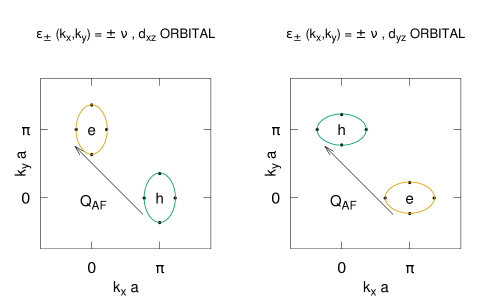
Figure 4: Shown are the the renormalized Fermi surface pockets for inter-band energy shift $\nu$ near the upper edge of the bonding band $\varepsilon_{+}({\bi k})$, and for $-\nu$ near the lower edge of the anti-bonding band $\varepsilon_{-}({\bi k})$. The orbital character is only approximate, although it becomes exact as the area of the Fermi surface pockets vanishes as $U_{0}$ diverges.

The second Eliashberg equation (5faobgb) can be evaluated in a similar way. After substituting in the simple pole in frequency for $U^{2}F_{0}(\Omega;\nu,\nu)$, integrating first over $\varepsilon^{\prime}$ yields the equation

$$\nu={\epsilon_{\rm E}\over 2}\int_{0}^{\omega_{\rm uv}}{d\Omega\over{\Omega}}{\rm ln}\Biggl{|}{(W/Z+\Omega)^{2}-\omega^{2}\over{\Omega^{2}-\omega^{2}}}\Biggr{|}.$$

Assuming, once again, the inequality $W/Z\gg\omega$ then yields the following equation in the low-frequency limit:

$$\nu=\epsilon_{\rm E}\int_{0}^{\omega_{\rm uv}}{d\Omega\over{\Omega}}{\rm ln}\Biggl{|}{W\over{\omega Z}}\Biggr{|}.$$

Here, we have expanded the previous argument of the logarithm in powers of $\Omega$. The final result for the second Eliashberg equation is then

$${\rm lim}_{\omega\rightarrow 0}\nu=\epsilon_{\rm E}\,{\rm ln}\Biggl{(}{\omega_{\rm uv}\over{\omega_{\rm ir}}}\Biggr{)}{\rm ln}\Biggl{(}{4\,W\over{\pi^{2}\epsilon_{\rm E}}}\Biggr{)},$$ (5faobgbm)

where $\omega_{\rm ir}\sim c_{0}/L$ is an infra-red cutoff in frequency. Above, the previous result from the first Eliashberg equation has been substituted in. We can now check the previous inequality that was assumed. The second Eliashberg equation (5faobgbm) implies that the energy scale (5faobgbj) is of order $\epsilon_{\rm E}\sim\varepsilon_{+}(\pi/a,0)/{\rm ln}(\omega_{\rm uv}/\omega_{\rm ir})$ for $\nu$ near the upper edge of the bonding band $\varepsilon_{+}({\bi k})$. The ratio $W/\omega Z=4W/\pi^{2}\epsilon_{\rm E}$ is therefore of order ${\rm ln}(\omega_{\rm uv}/\omega_{\rm ir})$, which diverges logarithmically as the infra-red cutoff in frequency $\omega_{\rm ir}$ tends to zero.

We shall finally estimate the Eliashberg energy scale (5faobgbj) $\epsilon_{\rm E}$. For simplicity, assume small circular Fermi surface pockets ($t_{1}^{\parallel}=0$) of Fermi radius $k_{F}$, which is related to the concentration $x_{0}$ of electron/holes per pocket by $k_{F}a=(2\pi x_{0})^{1/2}$. The Fermi velocity is then $v_{F}=2t_{1}^{\perp}k_{F}a^{2}$. Also, the phase shift (5fb) is approximately $\sin\,2\delta({\bi k})=[(t_{2}^{\perp}/i)/2t_{1}^{\perp}](k_{F}a)^{2}\,\sin\,2\phi$, where $\phi$ is the angle that ${\bi k}$ makes about the center of the Fermi surface pocket at $(\pi/a,0)$ or at $(0,\pi/a)$. We then get the expression

$$\epsilon_{\rm E}={1\over 16}\Biggl{(}{x_{0}\over{2\pi}}\Biggr{)}^{3/2}{U^{2}(\pi)\over{a^{2}D_{+}(\nu)}}{s_{1}^{2}\over{a^{2}\chi_{\perp}}}{|t_{2}^{\perp}|^{2}\over{(c_{0}/a)|t_{1}^{\perp}|^{4}}}$$ (5faobgbn)

for the Eliashberg energy scale (5faobgbj). Comparing this estimate with the second Eliashberg equation (5faobgbm), while fixing $\nu$ to the upper edge of the band ${\varepsilon}_{+}({\bi k})$, then yields that the area of the electron/hole Fermi surface pockets shown in Fig. 4 vanishes logarithmically with the size $L$ of the system for any positive $U(\pi)$. Note, however, that such behavior is effectively ruled out at the weak-coupling limit, $U(\pi)\rightarrow 0$, because the ordered magnetic moment $s_{1}$ vanishes exponentially in such case. On the other hand, if instead the scale $L$ of the system is fixed, then the previous comparison of (5faobgbm) and (5faobgbn) yields $U(\pi)\propto x_{0}^{-3/4}$. By the previous estimate for the phase shift at the new Fermi surface pockets, the electron-hidden-spin-wave interaction (5faoav) then scales as $U(\pi)^{-1/3}$. This justifies our neglect of vertex corrections at the limit of strong on-site repulsion, $U_{0}\rightarrow\infty$.

Last, a self-consistent solution to the above Eliashberg equations at the limit of large on-iron-site-orbital Coulomb repulsion, $U_{0}$, also exists at a relative shift of the bands $\nu$ near the bottom edge of the bonding band, $\varepsilon_{+}({\bi k})$, instead. In particular, $[\nu,\nu+W]$ is now the range of integration over $\varepsilon^{\prime}$ in the Eliashberg equations (5faobga) and (5faobgb). The previous results for the wavefunction renormalization (5faobgbl) and for the relative energy shift between the two bands (5faobgbm) hold after making the replacement $\nu=W_{\rm top}$ with $-\nu=W_{\rm bottom}$ in the latter. It is important, now, to observe that the density of states of the bonding band at the upper band edge is larger than the density of states at the bottom edge by Fig. 2. The condensation energy is of order $-D_{+}(\nu)\Delta_{0}^{2}$, however. By the definition (5fw) for $\Delta_{0}$ and by Fig. 3 for the ordered magnetic moment, the condensation energy dominates the kinetic (hopping) energy at strong on-site repulsion $U_{0}$ compared to the bandwidth. This argues in favor of the former solution in such case, with $\nu$ at the upper edge of the band $\varepsilon_{+}({\bi k})$.

5 Discussion

The previous mean field theory analysis of the extended two-orbital Hubbard model for heavily electron-doped FeSe finds that hidden Néel antiferromagnetic order is expected at perfect nesting (5fg) $t_{2}^{\parallel}=0$ when true Néel order is suppressed by magnetic frustration[24, 25]. (See Figs. 1 and 4.) Below, we compare the observable consequences that have been listed above with analogous theoretical results at the strong-coupling limit[18], $U_{0}\rightarrow\infty$, and with recent experimental evidence for such hidden magnetic order in the superconducting state of intercalated FeSe[20, 21, 22]. We also argue why the effects of the iron $3d_{xy}$ orbital can be neglected.

5.1 Comparison of weak coupling and strong coupling

In subsections 3.3 and 3.4, we showed how mean field theory for the hidden Néel state of the two-orbital Hubbard model that describes heavily electron-doped FeSe agrees both qualitatively and quantitatively with the corresponding Heisenberg model at large on-iron-site-orbital repulsion. In particular, a hydrodynamical analysis (5fai) predicts two acoustically dispersing spin-wave excitations per momentum near the “checkerboard” wavenumber ${\bi Q}_{\rm AF}$. This agrees with the large-$s_{0}$ analysis of the corresponding Heisenberg model[25]. Second, the transverse spin susceptibility of the hSDW state (5fak) was calculated above as well. At weak hybridization between the $3d_{xz}$ and $3d_{yz}$ orbitals, the transverse susceptibility of the hSDW state at the limit of strong on-iron-site-orbital Coulomb repulsion (5faoap) is found to agree with the same quantity calculated from the corresponding Heisenberg model in the large-$s_{0}$ limit[25]. Also, the spin rigidity (5faoaq) of the hSDW state was computed above at the limit of strong on-iron-site-orbital repulsion. A comparison with the same results for the corresponding Heisenberg model (5faobgbo) yields exchange coupling constants that are consistent with hidden Néel order. (See the Goldstone mode in Fig. 5b.)

Figure 4 is the central result of the paper, however. It shows the Fermi surfaces of the extended Hubbard model in the hSDW state at half-filling and at strong on-iron-site-orbital Coulomb repulsion, as predicted by Eliashberg theory in the particle-hole channel. The rigid-band approximation, in turn, predicts electron-type Fermi surface pockets alone at wavenumbers $(\pi/a,0)$ and $(0,\pi/a)$ upon electron doping at concentrations per pocket $x>x_{0}$. Here, $x_{0}$ denotes the concentration of electrons/holes inside the Fermi surface pockets shown in Fig. 4. It vanishes as $U_{0}$ diverges. This argument agrees with Schwinger-boson-slave-fermion mean field theory of the corresponding local-moment ($t$-$J$) model at electron doping[18], in which case $U_{0}\rightarrow\infty$ and $x_{0}\rightarrow 0$, and in which case only the electron-type Fermi surface pockets shown in Fig. 4 appear. It also notably agrees with ARPES on heavily electron-doped FeSe[5, 6, 8, 9]. In particular, $x_{0}$ may represent a threshold concentration of electron doping at which hSDW order gives way to superconductivity.

5.2 Comparison of hidden magnetic order with experiment

The local-moment limit of the present extended Hubbard model for heavily electron-doped FeSe is achieved at strong on-site-orbital repulsion, $U_{0}\rightarrow\infty$. At half filling, it results in a two-orbital Heisenberg model over the square lattice of the form[25]

$$H_{\rm Hsnbrg}= \sum_{\langle i,j\rangle}\sum_{\alpha}(J_{1}^{\parallel}{\bi S}_{i,\alpha}\cdot{\bi S_{j,\alpha}}+J_{1}^{\perp}{\bi S}_{i,\alpha}\cdot{\bi S}_{j,{\bar{\alpha}}})$$ (5faobgbo)

$$+\sum_{\langle\langle i,j\rangle\rangle}\sum_{\alpha}(J_{2}^{\parallel}{\bi S}_{i,\alpha}\cdot{\bi S_{j,\alpha}}+J_{2}^{\perp}{\bi S}_{i,\alpha}\cdot{\bi S}_{j,\bar{\alpha}}),$$

where $\alpha=d-$ or $d+$. In particular, the results obtained in subsection 3.4 for the transverse spin susceptibility and for the spin rigidity of the hSDW state are consistent with the following assignments for the Heisenberg exchange coupling constants: $J_{1}^{\parallel}=J_{1}^{({\rm sprx})}$, $J_{1}^{\perp}=J_{1}^{({\rm sprx})}-\rho_{s}/2s_{0}^{2}$, and $J_{2}^{\parallel}=J_{2}^{({\rm sprx})}=J_{2}^{\perp}$. Here, $\rho_{s}>0$ is the spin rigidity of the hSDW (5faoar). Adding electrons at this strong-coupling limit can be studied analytically within the Schwinger-boson-slave-fermion formulation when only inter-orbital nearest neighbor hopping, $t_{1}^{\perp}>0$, exists[18]. The mean field theory of the corresponding hSDW state is well behaved in such case. As mentioned previously, it shows two electron-type Fermi surface pockets at the corner of the two-iron Brillouin zone, with $3d_{xz}$ and $3d_{yz}$ orbital character respectively. (Cf. Fig. 4.) Schwinger-boson-slave-fermion mean field theory also finds two branches of spin-wave excitations that correspond to true and to hidden magnetic moments, ${\bi S}_{i,d-}+{\bi S}_{i,d+}$ and ${\bi S}_{i,d-}-{\bi S}_{i,d+}$, respectively. They are governed by the Heisenberg model (5faobgbo) in the large-$s_{0}$ limit, but with the replacement $J_{1}^{\perp}\rightarrow J_{1}^{\perp}-t_{1}^{\perp}x/(1-x)^{2}s_{0}$. Here, $s_{0}$ is the electron spin, and $x$ is the electron doping concentration per site-orbital. Figure 5 shows the spin-wave spectra from such a large-$s_{0}$ approximation for the hSDW state of the local-moment model near a critical Hund’s Rule coupling $J_{0c}$ where the spectrum softens completely at “stripe” SDW wavenumbers $(\pi/a,0)$ and $(0,\pi/a)$ [18]; i.e., $\Delta_{\rm cSDW}\rightarrow 0$.

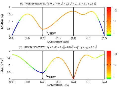
Figure 5: Spin-excitation spectrum for hidden spin-density-wave state of the Heisenberg model (5faobgbo) at the large-$s_{0}$ limit, but with the replacement $J_{1}^{\perp}\rightarrow J_{1}^{\perp}-t_{1}^{\perp}x/(1-x)^{2}s_{0}$. (See refs. [18, 25] and the main text.) Here, $s_{0}=1/2$, $t_{1}^{\perp}=5\,J_{1}^{\parallel}$ and $x=0.01$.

The results shown by Fig. 5 for the spin-excitation spectrum of the hSDW state are obtained from the local-moment model for heavily electron-doped FeSe that includes only inter-orbital nearest neighbor hoping, $t_{1}^{\perp}>0$. The $3d_{xz}$ and $3d_{yz}$ orbitals are good quantum numbers in such case. In particular, they are respectively even and odd under swap of the $d-$ and the $d+$ orbitals, $P_{d,{\bar{d}}}$. Likewise, the true and hidden magnetic moments just cited are respectively even and odd under[37] $P_{d,{\bar{d}}}$. Unfortunately, unlike the previous analysis of the extended Hubbard model, the Schwinger-boson-slave-fermion mean field theory that such results are based on is not well behaved when mixing between the two orbitals (pure imaginary $t_{2}^{\perp}$) is turned on[18]. Orbital swap $P_{d,{\bar{d}}}$ is no longer a global symmetry in such case. Figure 6 shows, however, the points in momentum and energy at which the two branches of the spin-excitation spectrum are degenerate. It reveals a “floating ring” of low-energy magnetic excitations about the Néel wave number ${\bi Q}_{\rm AF}$. Observable spin excitations should be brightest along the floating ring at weak mixing between the $3d_{xz}$ and $3d_{yz}$ orbitals. Similar low-energy spin resonances around ${\bi Q}_{\rm AF}$ have been observed recently in the superconducting phase of intercalated FeSe by inelastic neutron scattering[20, 21, 22]. Such experiments are then consistent with the hSDW state proposed here for heavily electron-doped FeSe.

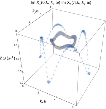
Figure 6: Curves in momentum versus energy where the dispersion of true spinwaves is degenerate with that of hidden spinwaves: $\omega_{b}(0,{\bi k})=\omega_{b}(\pi,{\bi k})$. Parameters for the Heisenberg model (5faobgbo) are listed in Fig. 5.

5.3 Iron $3d_{xy}$ Orbital

In addition to the iron $3d_{xz}$ and $3d_{yz}$ orbitals considered in the present extended Hubbard model, ARPES on iron chalcogenides coupled with density-functional theory calculations indicate that the iron $3d_{xy}$ orbital also plays an important role in the electronic structure[47]. Without loss of generality, let us then simply add this orbital to the four on-site terms in $H_{U}$ (5fq) and to both super-exchange terms in $H_{\rm sprx}$ (5fr). Next, let us work within the approximation that no hybridization exists in between the $3d_{xy}$ band, $\varepsilon_{xy}({\bi k})$, and the $3d_{xz}/3d_{yz}$ bands, $\varepsilon_{-}({\bi k})$ and $\varepsilon_{+}({\bi k})$. Assume also that the $3d_{xy}$ band shows no nesting. Now recall that the net magnetic moment due to the $3d_{xz}/3d_{yz}$ orbitals is null in the hidden magnetic order state. This implies that the paramagnetic state for electrons in the $3d_{xy}$ orbital, $\langle n_{i,d_{xy},\uparrow}\rangle=\langle n_{i,d_{xy},\downarrow}\rangle$, is stable within the mean-field approximation outlined in subsection 3.2. The paramagnetic state of $3d_{xy}$ electrons is thereby decoupled from the $3d_{xz}/3d_{yz}$ electrons in the hidden magnetic order state. The former then acts as a potential charge reservoir for the latter. What happens in the case where hybridization exists between all three orbitals[36] remains an open question that lies outside the scope of the present study.

6 Summary and Conclusions

Understanding the mechanism behind the high-temperature superconductivity displayed by heavily electron-doped iron selenide remains elusive. In an attempt to solve this mystery, we have shown how the electron-type Fermi surface pockets that exist at the corner of the two-iron Brillouin zone in heavily electron-doped iron-selenide can emerge from an extended Hubbard model over the square lattice of iron atoms that includes only the $3d_{xz}$ and $3d_{yz}$ orbitals. At half-filling, and in the absence of next-nearest neighbor intra-orbital hopping, perfect nesting exists between hole-type and electron-type Fermi surfaces displayed by Fig. 1. The nesting wavenumber is $(\pi/a,\pi/a)$, which corresponds to checkerboard (Néel) order. It notably differs from parent compounds to iron-pnictide high-temperature superconductors, which display “stripe” spin-density order, with nesting vector $(\pi/a,0)$. The former checkerboard nesting can lead to hidden Néel order that violates Hund’s Rule when true Néel order is suppressed by magnetic frustration[24, 25]. An extended Hartree-Fock calculation of the Eliashberg type reveals that hole and electron Fermi surfaces become centered at the corner of the two-iron Brillouin zone at moderate to strong on-site Coulomb repulsion because of the exchange of antiferromagnetic spin fluctuations. The electron/hole concentration $x_{0}$ that corresponds to the area of these Fermi surface pockets vanishes as the on-site Coulomb repulsion diverges. Sufficiently strong electron doping $x>x_{0}$ will then produce a rigid shift of such a renormalized band structure, with electron Fermi surface pockets alone that are similar to those seen by ARPES in heavily electron-doped FeSe.

We have also shown that the extended two-orbital Hubbard model leads to a local-moment model in the limit of strong on-site Coulomb repulsion that harbors the same type of hidden magnetic order[25]. Recent calculations by one of the authors also find electron-type Fermi surface pockets at the corner of the two-iron Brillouin zone when electrons are added to the local moments[18]. Furthermore, in the previous section, we have pointed out that the low-energy spin excitations predicted by the local-moment model in the hidden magnetic order phase resemble the “floating” ring of spin-excitations that has been observed recently in heavily electron-doped FeSe by inelastic neutron scattering[20, 21, 22]. The extended two-orbital Hubbard model therefore is promising phenomenologically.

Yet does it harbor superconductivity? Recent exact calculations by one of the authors on finite clusters at the local-moment limit find evidence for Cooper pairs near a quantum critical point to “stripe” spin-density wave order[18]. Also, quantum Monte Carlo simulations of a spin-fluctuation-exchange model that is free of the sign problem, and that is very similar to the model studied here [Eqs. (1), (5faoat), and (5faoau)], find evidence for competition between SDW and superconducting groundstates[48]. (See also refs. [49] and [50].) It remains to be seen if the extended Hubbard model introduced here also harbors superconductivity away from half filling, and if so, of what type.

Appendix A Particle-Hole Symmetry

Let us turn off next-nearest neighbor intra-orbital hopping (1), $t_{2}^{\parallel}=0$. Consider then the following particle-hole transformation:

$$c_{i,d\pm,s}\rightarrow e^{i{\bi Q}_{\rm AF}\cdot{\bi r}_{i}}c_{i,d\mp,s}^{\dagger},$$

$$c_{i,d\pm,s}^{\dagger}\rightarrow e^{-i{\bi Q}_{\rm AF}\cdot{\bi r}_{i}}c_{i,d\mp,s},$$ (5faobgbp)

where ${\bi Q}_{\rm AF}=(\pi/a,\pi/a)$. Making the above replacements in the Hamiltonian $H_{\rm hop}+H_{U}+H_{\rm sprx}$ for the extended two-orbital Hubbard model over the square lattice (1,5fq,5fr) then results in the same Hamiltonian back up to a constant energy shift and up to a shift in the chemical potential. The extended two-orbital Hubbard model $H_{\rm hop}+H_{U}+H_{\rm sprx}$ is therefore symmetric under the particle-hole transformation (5faobgbp) at $t_{2}^{\parallel}=0$.

Next, substitution of the above particle-hole transformation (5faobgbp) into the creation operator for band electrons (5fh) yields the equivalent transformation in momentum space:

$$c_{s}(n,{\bi k})\rightarrow\pm i\,c_{s}^{\dagger}({\bar{n}},{\bar{\bi k}}),$$

$$c_{s}^{\dagger}(n,{\bi k})\rightarrow\mp i\,c_{s}({\bar{n}},{\bar{\bi k}}),$$ (5faobgbq)

where ${\bar{n}}=1+(n\;{\rm mod}\;2)$, and where ${\bar{\bi k}}={\bi k}+{\bi Q}_{\rm AF}$. Here, we have used the property

$$\delta({\bi k}+{\bi Q}_{\rm AF})=\pm{\pi\over 2}-\delta({\bi k})$$ (5faobgbr)

satisfied by the phase shift, which is a result of the property $\varepsilon_{\perp}({\bi k}+{\bi Q}_{\rm AF})=-\varepsilon_{\perp}^{*}({\bi k})$ satisfied by the matrix element (5b). The hopping Hamiltonian (1) is expressed in momentum space as

$$H_{\rm hop}=\sum_{\bi k}\sum_{n}\sum_{s}\varepsilon_{n}({\bi k})c_{s}^{\dagger}(n,{\bi k})c_{s}(n,{\bi k}).$$

It is invariant under the particle-hole transformation (5faobgbq) if the perfect nesting condition (5fg) at $t_{2}^{\parallel}=0$ holds true. Here, we have used the property $\sum_{\bi k}\sum_{n}\varepsilon_{n}({\bi k})=0$.

Appendix B Antiferromagnetic magnetization and matrix elements

Substituting the identity (5fi) for the creation operator into expression (5fj) for the antiferromagnetic magnetization, along with the conjugate expression for the destruction operator, yields the form

$$S_{z}(m,{\bi Q}_{\rm AF})={1\over 2}\sum_{s}\sum_{\bi k}\sum_{n,n^{\prime}}({\rm sgn}\,s){\cal M}_{n,{\bi k};n^{\prime},{\bar{\bi k}}}c_{s}^{\dagger}(n^{\prime},{\bar{\bi k}})c_{s}(n,{\bi k}),$$

(5faobgbs)

with ${\bar{\bi k}}={\bi k}+{\bi Q}_{\rm AF}$, and with matrix element

$${\cal M}_{n,{\bi k};n^{\prime},{\bi k}^{\prime}}={1\over 2}\sum_{\alpha=0,1}e^{i(2\alpha-1)[\delta({\bi k})-\delta({\bi k}^{\prime})]}(-1)^{(n^{\prime}-n+m)\alpha}.$$ (5faobgbt)

The matrix element therefore equals

$${\cal M}_{n,{\bi k};n^{\prime},{\bi k}^{\prime}}=\cases{\cos[\delta({\bi k})-\delta({\bi k}^{\prime})]&for $n^{\prime}=n+m\;({\rm mod}\;2)$,\\ -i\,\sin[\delta({\bi k})-\delta({\bi k}^{\prime})]&for $n^{\prime}=n+m+1\;({\rm mod}\;2)$.}$$ (5faobgbu)

Now replace ${\bi k^{\prime}}$ above with ${\bar{\bi k^{\prime}}}={\bi k^{\prime}}+{\bi Q}_{\rm AF}$, and recall the definition of the phase shift: $e^{i2\delta}=\varepsilon_{\perp}/|\varepsilon_{\perp}|$. Inspection of (5b) yields the identity $\varepsilon_{\perp}({\bar{\bi k}})=-\varepsilon_{\perp}^{*}({\bi k})$, which in turn yields the identity (5faobgbr). It implies that $\delta({\bi k})-\delta({\bar{\bi k^{\prime}}})=\delta({\bi k})+\delta({\bi k^{\prime}})\mp\pi/2$. Substituting this into the previous result (5faobgbu) for the matrix element yields the final result

$${\cal M}_{n,{\bi k};n^{\prime},{\bar{\bi k^{\prime}}}}=\cases{\pm\sin[\delta({\bi k})+\delta({\bi k^{\prime}})]&for $n^{\prime}=n+m\;({\rm mod}\;2)$,\\ \pm i\,\cos[\delta({\bi k})+\delta({\bi k^{\prime}})]&for $n^{\prime}=n+m+1\;({\rm mod}\;2)$.}$$ (5faobgbv)

Appendix C Transverse spin susceptibility

Let us add a term $-h\sum_{i}\sum_{\alpha}S_{i,\alpha}^{(y)}$ to the mean-field Hamiltonian (5fx) in the text. Here, $h$ represents an external magnetic field applied along the $y$ axis that is perpendicular to the sub-lattice magnetization of the hidden antiferromagnet, which points along the $z$ axis. Following the discussion in section 3.3, we shall quantize spin along the $y$-axis instead: $z^{\prime}=y$, $x^{\prime}=z$ and $y^{\prime}=x$. The mean-field Hamiltonian (5fx) plus the additional terms above then becomes

$$H^{(mf)}=\sum_{s}\sum_{\bi k}\left[{\begin{array}[]{c}c_{s}^{\prime}\\ {\bar{c}}_{\bar{s}}^{\prime}\end{array}}\right]^{\dagger}\left[{\begin{array}[]{cc}\varepsilon_{+}-({\rm sgn}\,s){1\over 2}h&\Delta\\ \Delta&-\varepsilon_{+}+({\rm sgn}\,s){1\over 2}h\end{array}}\right]\left[{\begin{array}[]{c}c_{s}^{\prime}\\ {\bar{c}}_{\bar{s}}^{\prime}\end{array}}\right]$$ (5faobgbw)

where $c_{s}^{\prime}({\bi k})=c_{s}^{\prime}(2,{\bi k})$, and where ${\bar{c}}_{s}^{\prime}({\bi k})=c_{s}^{\prime}(1,{\bi k}+{\bi Q}_{\rm AF})$. Above, ${\bar{s}}=-s$. The energy eigenvalues of the quasi-particle excitations are then

$$E_{s}({\bi k})=\sqrt{[\varepsilon_{+}({\bi k})-({\rm sgn}\,s){1\over 2}h]^{2}+\Delta^{2}({\bi k})},$$ (5faobgbx)

with $\Delta({\bi k})=\Delta_{0}[\sin\,2\delta({\bi k})]$. The transverse magnetization per iron atom is then

$$M_{y} = {1\over 2}(a^{2}N_{\rm Fe})^{-1}\sum_{s}\sum_{\bi k}\sum_{n}({\rm sgn}\,s)\langle c_{s}^{\prime\dagger}(n,{\bi k})c_{s}^{\prime}(n,{\bi k})\rangle$$ (5faobgby)

$$= {1\over 2}(a^{2}N_{\rm Fe})^{-1}\sum_{\bi k}\sum_{s}({\rm sgn}\,s)[v_{s}^{2}({\bi k})-u_{s}^{2}({\bi k})],$$

where $u_{s}^{2}={1\over 2}+{1\over 2}[\varepsilon_{+}-({\rm sgn}\,s){1\over 2}h]/E_{s}$ and $v_{s}^{2}={1\over 2}-{1\over 2}[\varepsilon_{+}-({\rm sgn}\,s){1\over 2}h]/E_{s}$. Substituting the latter in above then yields

$$M_{y}={1\over 2}(a^{2}N_{\rm Fe})^{-1}\sum_{\bi k}\Biggl{(}-{\varepsilon_{+}-{1\over 2}h\over{E_{\uparrow}}}+{\varepsilon_{+}+{1\over 2}h\over{E_{\downarrow}}}\Biggr{)}.$$ (5faobgbz)

Finally, taking the limit $h\rightarrow 0$ above results in the linear response $M_{y}=\chi_{\perp}^{(0)}h$, with transverse spin susceptibility

$$\chi_{\perp}^{(0)}={1\over 2}(a^{2}N_{\rm Fe})^{-1}\sum_{\bi k}{\Delta^{2}\over E^{3}}.$$ (5faobgca)

We will next prove that the integrals $I_{1}$ and $I_{2}$ defined by (5faoa) and (5faob) can only be equal in the limit $t_{2}^{\perp}\rightarrow 0$ as $U_{0}\rightarrow\infty$. First, observe that inspection of (5fb) yields the limit ${\rm lim}_{t_{2}^{\perp}\rightarrow 0}\sin\,2\delta({\bi k})=0$. Next, observe by (5faoa) that the limit ${\rm lim}_{U_{0}\rightarrow\infty,t_{2}^{\perp}\rightarrow 0}I_{1}$ is equal to

$${\rm lim}_{U_{0}\rightarrow\infty,t_{2}^{\perp}\rightarrow 0}{1\over 2}N_{\rm Fe}^{-1}\sum_{\bi k}([\varepsilon_{+}({\bi k})/U(\pi)]^{2}+[\langle m_{0,0}\rangle\sin\,2\delta({\bi k})]^{2})^{-1/2}.$$

Figure 3 indicates that the hidden magnetic moment $\langle m_{0,0}\rangle$ vanishes roughly as the hybridization between the $3d_{xz}$ and $3d_{yz}$ orbitals, $|t_{2}^{\perp}|$. We conclude that the limit ${\rm lim}_{U_{0}\rightarrow\infty,t_{2}^{\perp}\rightarrow 0}I_{1}$ diverges at least linearly with $U_{0}$. Second, observe that the quotient in expression (5faob) for $I_{2}$ is equal to $2\,\delta(\Delta_{0}[\sin\,2\delta({\bi k})])$ in the limit $U_{0}\rightarrow\infty$. By (5fw), this yields the limiting expression

$${\rm lim}_{U_{0}\rightarrow\infty}I_{2}=a^{2}\int_{-\pi/a}^{+\pi/a}{dk_{x}\over{2\pi}}\int_{-\pi/a}^{+\pi/a}{dk_{y}\over{2\pi}}\delta(\langle m_{0,0}\rangle[\sin\,2\delta({\bi k})]),$$ (5faobgcb)

which coincides with the product of $a^{2}U(\pi)$ with the density of states of $\Delta_{0}[\sin\,2\delta({\bi k})]$ at zero energy. Now notice by (5fb) that $\sin\,2\delta({\bi k})$ disperses hyperbolically near $(\pi/a,0)$ and $(0,\pi/a)$. This implies that ${\rm lim}_{U_{0}\rightarrow\infty,t_{2}^{\perp}\rightarrow 0}I_{2}$ diverges roughly as $(|t_{1}^{\perp}|/|t_{2}^{\perp}|)^{2}{\rm ln}[U(\pi)/W_{\rm bottom}]$. Equating $I_{1}$ with $I_{2}$ then yields that $t_{2}^{\perp}\rightarrow 0$ as $U_{0}\rightarrow\infty$, which is consistent with the original assumption.

Appendix D Eliashberg equations at non-zero temperature

Equation (LABEL:E_eqs_T) in the text lists the three Eliashberg equations at non-zero temperature in terms of sums over Matsubara frequencies. The sums can be evaluated in closed form after a series of decompositions into partial fractions. That procedure yields

$$[Z({\bi k},\omega)-1]\omega = \int{d^{2}k^{\prime}\over{(2\pi)^{2}}}{U^{2}(\pi)\over 2}{(2s_{1})^{2}\over{\chi_{\perp}}}{\sin^{2}[\delta({\bi k})+\delta({\bi k}^{\prime})]\over{2Z({\bi k}^{\prime},\omega)\cdot 2\omega_{b}({\bi q})}}\cdot$$

$$\ \Biggl{\{}(n_{\rm F}[-E({\bi k}^{\prime})]+n_{\rm B}[\omega_{b}({\bi q})])\cdot$$

$$\ \ \ \cdot\Biggl{[}{1\over{\omega_{b}({\bi q})+E({\bi k}^{\prime})-\omega}}-{1\over{\omega_{b}({\bi q})+E({\bi k}^{\prime})+\omega}}\Biggr{]}+$$

$$\ \ \ (n_{\rm F}[+E({\bi k}^{\prime})]+n_{\rm B}[\omega_{b}({\bi q})])\cdot$$

$$\ \ \ \cdot\Biggl{[}{1\over{\omega_{b}({\bi q})-E({\bi k}^{\prime})-\omega}}-{1\over{\omega_{b}({\bi q})-E({\bi k}^{\prime})+\omega}}\Biggr{]}\Biggr{\}},$$

$$-\nu = \int{d^{2}k^{\prime}\over{(2\pi)^{2}}}{U^{2}(\pi)\over 2}{(2s_{1})^{2}\over{\chi_{\perp}}}{\sin^{2}[\delta({\bi k})+\delta({\bi k}^{\prime})]\over{2Z({\bi k}^{\prime},\omega)\cdot 2\omega_{b}({\bi q})}}{\varepsilon_{+}({\bi k}^{\prime})-\nu\over{Z({\bi k}^{\prime},\omega)E({\bi k}^{\prime})}}\cdot$$

$$\ \Biggl{\{}(n_{\rm F}[-E({\bi k}^{\prime})]+n_{\rm B}[\omega_{b}({\bi q})])\cdot$$

$$\ \ \ \cdot\Biggl{[}{1\over{\omega_{b}({\bi q})+E({\bi k}^{\prime})-\omega}}+{1\over{\omega_{b}({\bi q})+E({\bi k}^{\prime})+\omega}}\Biggr{]}-$$

$$\ \ \ (n_{\rm F}[+E({\bi k}^{\prime})]+n_{\rm B}[\omega_{b}({\bi q})])\cdot$$

$$\ \ \ \cdot\Biggl{[}{1\over{\omega_{b}({\bi q})-E({\bi k}^{\prime})-\omega}}+{1\over{\omega_{b}({\bi q})-E({\bi k}^{\prime})+\omega}}\Biggr{]}\Biggr{\}},$$

$$Z({\bi k},\omega)\Delta({\bi k}) = \int{d^{2}k^{\prime}\over{(2\pi)^{2}}}{U^{2}(\pi)\over 2}{(2s_{1})^{2}\over{\chi_{\perp}}}{\sin^{2}[\delta({\bi k})+\delta({\bi k}^{\prime})]\over{2Z({\bi k}^{\prime},\omega)\cdot 2\omega_{b}({\bi q})}}{\Delta({\bi k}^{\prime})\over{E({\bi k}^{\prime})}}\cdot$$

$$\ \ \ \ \Biggl{\{}(n_{\rm F}[-E({\bi k}^{\prime})]+n_{\rm B}[\omega_{b}({\bi q})])\cdot$$

$$\ \ \ \ \ \ \ \cdot\Biggl{[}{1\over{\omega_{b}({\bi q})+E({\bi k}^{\prime})-\omega}}+{1\over{\omega_{b}({\bi q})+E({\bi k}^{\prime})+\omega}}\Biggr{]}-$$

$$\ \ \ \ \ \ (n_{\rm F}[+E({\bi k}^{\prime})]+n_{\rm B}[\omega_{b}({\bi q})])\cdot$$

$$\ \ \ \ \ \cdot\Biggl{[}{1\over{\omega_{b}({\bi q})-E({\bi k}^{\prime})-\omega}}+{1\over{\omega_{b}({\bi q})-E({\bi k}^{\prime})+\omega}}\Biggr{]}\Biggr{\}}.$$

Above, ${\bi q}={\bi k}-{\bi k}^{\prime}-{\bi Q}_{\rm AF}$. Also, $n_{\rm F}(\varepsilon)$ and $n_{\rm B}(\omega)$ denote the Fermi-Dirac and the Bose-Einstein distribution functions.

References

- [1] Y. Kamihara, T. Watanabe, M. Hirano, and H. Hosono, J. Am. Chem. Soc. 130, 3296 (2008).
- [2] W.-H. Zhang, Y. Sun, J.-S. Zhang, F.-S. Li, M.-H. Guo, Y.-F. Zhao, H.-M. Zhang, J.-P. Peng, Y. Xing, H.-C. Wang, T. Fujita, A. Hirata, Z. Li, H. Ding, C.-J. Tang, M. Wang, Q.-Y. Wang, K. He, S.-H. Ji, X. Chen, J.-F. Wang, Z.-C. Xia, L. Li, Y.-Y. Wang, J. Wang, L.-L. Wang, M.-W. Chen, Q.-K. Xue, and X.-C. Ma, Chin. Phys. Lett. 31, 017401 (2014).
- [3] J.-F. Ge, Z.-L. Liu, C. Liu, C.-L. Gao, D. Qian, Q.-K. Xue, Y. Liu, J.-F. Jia, Nat. Mater. 14, 285 (2015).
- [4] Q.-Y. Wang, Z. Li, W.-H. Zhang, Z.-C. Zhang, J.-S. Zhang, W. Li, H. Ding, Y.-B. Ou, P. Deng, K. Chang, J. Wen, C.-L. Song, K. He, J.-F. Jia, S.-H. Ji, Y. Wang, L. Wang, X. Chen, X. Ma, Q.-K. Xue, Chin. Phys. Lett. 29, 037402 (2012).
- [5] D. Liu, W. Zhang, D. Mou, J. He, Y.-B. Ou,Q.-Y. Wang, Z. Li, L. Wang, L. Zhao, S. He, Y. Peng, X. Liu, C. Chaoyu, L. Yu, G. Liu, X. Dong, J. Zhang, C. Chen, Z. Xu, J. Hu, X. Chen, Z. Ma, Q. Xue and X.J. Xhou, Nat. Comm. 3, 931 (2012).
- [6] S. He, J. He, W.-H. Zhang, L. Zhao, D. Liu, X. Liu, D. Mou, Y.-B. Ou, Q.-Y. Wang, Z. Li, L. Wang, Y. Peng, Y. Liu, C. Chen, L. Yu, G. Liu, X. Dong, J. Xhang, C. Chen, Z. Xu, X. Chen, X. Ma, Q. Xue, and X.J. Zhou, Nat. Mater. 12, 605 (2013).
- [7] Q. Fan, W. H. Zhang, X. Liu, Y.J. Yan, M.Q. Ren, R. Peng, H. C. Xu, B. P. Xie, J. P. Hu, T. Zhang, and D. L. Feng, Nat. Phys. 11, 946 (2015).
- [8] L. Zhao, A. Liang, D. Yuan, Y. Hu, D. Liu, J. Huang, S. He, B. Shen, Y. Xu, X. Liu, L. Yu, G. Liu, H. Zhou, Y. Huang, X. Dong, F. Zhou, Z. Zhao, C. Chen, Z. Xu, X.J. Zhou, Nat. Comm. 7, 10608 (2016).
- [9] X.H. Niu, R. Peng, H.C. Xu, Y.J. Yan, J. Jiang, D.F. Xu, T.L. Yu, Q. Song, Z.C. Huang, Y.X. Wang, B.P. Xie, X.F. Lu, N.Z. Wang, X.H. Chen, Z. Sun, and D.L. Feng, Phys. Rev. B 92, 060504(R) (2015).
- [10] Y. J. Yan, W. H. Zhang, M. Q. Ren, X. Liu, X. F. Lu, N. Z. Wang, X. H. Niu, Q. Fan, J. Miao, R. Tao, B. P. Xie, X. H. Chen, T. Zhang, D. L. Feng, Phys. Rev. B 94, 134502 (2016).
- [11] Y. Miyata, K. Nakayama, K. Suawara, T. Sato, and T. Takahashi, Nat. Mater. 14, 775 (2015).
- [12] C.H.P. Wen, H.C. Xu, C. Chen, Z.C. Huang, X. Lou, Y.J. Pu, Q. Song, B.P. Xie, M. Abdel-Hafiez, D.A. Chareev, A.N. Vasiliev, R. Peng, and D.L. Feng, Nat. Comm. 7, 10840, (2016).
- [13] C.-L. Song, H.-M. Zhang, Y. Zhong, X.-P. Hu, S.-H. Ji, L. Wang, K. He, X.-C. Ma, and Q.-K. Xue, Phys. Rev. Lett. 116, 157001 (2016).
- [14] B. Lei, J.H. Cui, Z.J. Xiang, C. Shang, N.Z. Wang, G.J. Ye, X.G. Luo, T. Wu, Z. Sun, and X.H. Chen, Phys. Rev. Lett. 116, 077002 (2016).
- [15] K. Hanzawa, H. Sato, H. Hiramatsu, T. Kamiya, and H. Hosono, Proc. Nat. Acad. Sci. 113, 3986 (2016).
- [16] J.J. Lee, F.T. Schmitt, R.G. Moore, S. Johnston, Y.-T. Cui, W. Li, M. Yi, Z.K. Liu, M. Hashimoto, Y. Zhang, D.H. Lu, T.P. Devereaux, D.-H. Lee and Z.-X. Shen, Nature 515, 245 (2014).
- [17] R. Peng, X.P. Shen, X. Xie, H.C. Xu, S.Y. Tan, M. Xia, T. Zhang, H.Y. Cao, X.G. Gong, J.P. Hu, B.P. Xie, D. L. Feng, Phys. Rev. Lett. 112, 107001 (2014).
- [18] J.P. Rodriguez, Phys. Rev. B 95, 134511 (2017).
- [19] D. Huang and J.E. Hoffman, Physics 9, 38 (2016).
- [20] N.R. Davies, M.C. Rahn, H.C. Walker, R.A. Ewings, D.N. Woodruff, S.J. Clarke, and A.T. Boothroyd, Phys. Rev. B 94, 144503 (2016).
- [21] B. Pan, Y. Shen, D. Hu, Y. Feng, J.T. Park, A.D. Christianson, Q. Wang, Y. Hao, H. Wo, and J. Zhao, Nat. Comm. 8, 123 (2017).
- [22] M. Ma, L. Wang, P. Bourges, Y. Sidis, S. Danilkin, and Y. Li, Phys. Rev. B 95, 100504(R) (2017).
- [23] J.P. Rodriguez, arXiv:1601.07479 .
- [24] J.P. Rodriguez and E.H. Rezayi, Phys. Rev. Lett. 103, 097204 (2009).
- [25] J.P. Rodriguez, Phys. Rev. B 82, 014505 (2010).
- [26] T. Bazhirov and M.L. Cohen, J. Phys.: Condens. Matter 25, 105506 (2013).
- [27] J.E. Hirsch, Phys. Rev. B 31, 4403 (1985).
- [28] J.R. Schrieffer, X.G. Wen, and S.C. Zhang, Phys. Rev. B 39, 11663 (1989).
- [29] A. Singh and Z. Tesanovic, Phys. Rev. B 41, 614 (1990).
- [30] A.V. Chubukov and D.M. Frenkel, Phys. Rev. B 46, 11884 (1992).
- [31] G.M. Eliashberg, Sov. Phys. JETP 11, 696 (1960).
- [32] G.M. Eliashberg, Sov. Phys. JETP 12, 1000 (1961).
- [33] J.R. Schrieffer, Theory of Superconductivity (Benjamin, New York, 1964).
- [34] D.J. Scalapino, in R.D. Parks (ed.) Superconductivity, vol. I (Dekker, New York, 1969).
- [35] S. Raghu, Xiao-Liang Qi, Chao-Xing Liu, D.J. Scalapino, Shou-Cheng Zhang, Phys. Rev. B 77, 220503(R) (2008).
- [36] P.A. Lee and X.-G. Wen, Phys. Rev. B 78, 144517 (2008).
- [37] J.P. Rodriguez, M.A.N. Araujo and P.D. Sacramento, Eur. Phys. J. B 87, 163 (2014).
- [38] M. Daghofer, A. Moreo, J.A. Riera, E. Arrigoni, D.J. Scalapino, and E. Dagotto, Phys. Rev. Lett. 101, 237004 (2008); A. Moreo, M. Daghofer, J.A. Riera, and E. Dagotto, Phys. Rev. B 79, 134502 (2009).
- [39] Y. Ran, F. Wang, H. Zhai, A. Vishwanath, D.-H. Lee, Phys. Rev. B 79, 014505 (2009).
- [40] P.W. Anderson, in Lectures on the Many-Body Problem, ed. E.R. Caianiello (Academic, Press, New York, 1964), vol. 2, p. 113.
- [41] B. I. Halperin and P. C. Hohenberg, Phys. Rev. 188, 898 (1969).
- [42] D. Forster, Hydrodynamic Fluctuations, Broken Symmetry, and Correlation Functions (Benjamin/Cummings, Reading, MA, 1975).
- [43] P.J.H. Denteneer, G. An, and J.M.J van Leeuwen, Phys. Rev. B 47, 6256 (1993).
- [44] Z.-P. Shi and R.P. Singh, Phys. Rev. B 52, 9620 (1995).
- [45] Y. Nambu, Phys. Rev. 117, 648 (1960).
- [46] L.P. Gorkov, Zh. Eksperim. i Teor. Fiz. 34, 735 (1958); Sov. Phys. JETP 7, 505 (1958).
- [47] M. Yi, Z-K Liu, Y. Zhang, R. Yu, J.-X. Zhu, J.J. Lee, R.G. Moore, F.T. Schmitt, W. Li, S.C. Riggs, J.-H. Chu, B. Lv, J. Hu, M. Hashimoto, S.-K. Mo, Z. Hussain, Z.Q. Mao, C.W. Chu, I.R. Fisher, Q. Si, Z.-X. Shen, and D.H. Lu, Nat. Comm. 6, 7777 (2015).
- [48] E. Berg, M. A. Metlitski, and S. Sachdev, Science 338, 1606 (2012).
- [49] Y. Schattner, M.H. Gerlach, S. Trebst, and E. Berg, Phys. Rev. Lett. 117, 097002 (2016).
- [50] Z.-X. Li, F. Wang, H. Yao, and D.-H. Lee, Sci. Bull. 61, 925 (2016).