Non-Markovianity and negative entropy production rates

Abstract

Entropy production plays a fundamental role in nonequilibrium thermodynamics to quantify the irreversibility of open systems. Its positivity can be ensured for a wide class of setups, but the entropy production rate can become negative sometimes. This is often taken as an indicator of non-Markovianity. We make this link precise by showing under which conditions a negative entropy production rate implies non-Markovianity and when it does not. For a system coupled to a single heat bath this can be established within a unified language for two setups: (i) the dynamics resulting from a coarse-grained description of a Markovian master equation and (ii) the classical Hamiltonian dynamics of a system coupled to a bath. The quantum version of the latter result is shown not to hold despite the fact that the integrated thermodynamic description is formally equivalent to the classical case. The instantaneous fixed point of a non-Markovian dynamics plays an important role in our study. Our key contribution is to provide a consistent theoretical framework to study the finite-time thermodynamics of a large class of dynamics with a precise link to its non-Markovianity.

I Introduction

The theory of stochastic processes provides a powerful tool to describe the dynamics of open systems. Physically, the noise to which these systems are subjected results from the fact that the system is coupled to an environment composed of many other degrees of freedom about which we have only limited information and control. This coarse-grained description of the system – as opposed to the microscopic description involving the composite system and environment – is particularly appealing and tractable, when the Markovian approximation is applied. Therefore, Markovian stochastic dynamics are nowadays very commonly used to describe small open systems ranging from biochemistry (e.g., enzymes, molecular motors) to quantum systems (e.g., single atoms or molecules) Hill (1977); Spohn (1980); van Kampen (2007); Breuer and Petruccione (2002). Due to their outstanding importance for many branches of science, an entire branch of mathematics is also devoted to their study Kemeny and Snell (1976).

A common feature of all Markovian processes is their contractivity, i.e., the volume of accessible states shrinks monotonically during the evolution. This statement can be made mathematically precise by considering two arbitrary preparations, $p_{\alpha}(0)$ and $q_{\alpha}(0)$, describing different probabilities to find the system in state $\alpha$ at the initial time $t=0$. Their distance, as measured by the relative entropy $D[p_{\alpha}\|q_{\alpha}]\equiv\sum_{\alpha}p_{\alpha}\ln\frac{p_{\alpha}}{q_{\alpha}}$, monotonically decreases over time $t$, i.e., for all $t\geq 0$

$$\frac{\partial}{\partial t}D[p_{\alpha}(t)\|q_{\alpha}(t)]\leq 0.$$ (1)

In other words, the ability to distinguish between any pair of initial states monotonically shrinks in time due to a continuous loss of information from the system to the environment. We note that also other distance quantifiers than the relative entropy fulfill Eq. (1) and an analogue of Eq. (1) also holds in the quantum regime where its violations has been proposed as an indicator of non-Markovianity Breuer et al. (2009); Rivas et al. (2014); Breuer et al. (2016).

The contractivity property (1) of Markov processes gets another interesting physical interpretation in quantum and stochastic thermodynamics. In these fields, a nonequilibrium thermodynamics is systematically build on top of Markovian dynamics typically described by (quantum) master or Fokker-Planck equations Schnakenberg (1976); Jiang et al. (2004); Esposito et al. (2009); Sekimoto (2010); Seifert (2012); Kosloff (2013); Schaller (2014); Van den Broeck and Esposito (2015). In addition to being Markovian, the rates entering the dynamics must also satisfy local detailed balance. For a system coupled to a single heat bath, this ensures that the Gibbs state of the system is a null eigenvector of the generator of the dynamics at all times $t$. For autonomous dynamics, this implies that the fixed point of the dynamics is an equilibrium Gibbs state. For nonautonomous (also called driven) dynamics, i.e., when some parameters are changed in time according to a prescribed protocol $\lambda_{t}$, the system in general does not reach a steady state, but the Gibbs state remains a null eigenvector of the generator of the dynamics at all times $t$. We call this an instantaneous fixed point of the dynamics in the following. If we denote the Gibbs state of the system by $e^{-\beta E_{\alpha}(\lambda_{t})}/{\cal{Z}}(\lambda_{t})$ with the energy $E_{\alpha}(\lambda_{t})$ of state $\alpha$ and the equilibrium partition function ${\cal{Z}}(\lambda_{t})=\sum_{\alpha}e^{-\beta E_{\alpha}(\lambda_{t})}$, the second law of thermodynamics for a driven system in contact with a single heat bath at inverse temperature $\beta$ can be expressed as

$$\dot{\Sigma}(t)=-\left.\frac{\partial}{\partial t}\right|_{\lambda_{t}}D\left[p_{\alpha}(t)\left\|\frac{e^{-\beta E_{\alpha}(\lambda_{t})}}{{\cal{Z}}(\lambda_{t})}\right.\right]\geq 0.$$ (2)

Here, the derivative is evaluated at fixed $\lambda_{t}$, i.e., $E_{\alpha}(\lambda_{t})$ and ${\cal{Z}}(\lambda_{t})$ are treated as constants, which only depend parametrically on time. The quantity $\dot{\Sigma}(t)$ is the entropy production rate. Its positivity follows from the fact that the dynamics is Markovian and that the Gibbs state is an instantaneous fixed point of the dynamical generator at all times. Within the conventional weak coupling and Markovian framework Schnakenberg (1976); Jiang et al. (2004); Esposito et al. (2009); Sekimoto (2010); Seifert (2012); Kosloff (2013); Schaller (2014); Van den Broeck and Esposito (2015), the entropy production rate can be rewritten as $\dot{\Sigma}(t)=\beta[\dot{W}(t)-d_{t}F(t)]\geq 0$, where $\dot{W}$ is the rate of work done on the system and $d_{t}F(t)$ denotes the change in non-equilibrium free energy (see Sec. III.1 for microscopic definitions of these quantities). The intimate connection between relative entropy and the second law was noticed some time ago in Ref. Procaccia and Levine (1976) for undriven systems. In the undriven case, the precise form of Eq. (2) seems to appear first in Ref. Spohn (1978) for quantum systems and it is discussed as a Lyapunov function in Ref. van Kampen (2007) for classical systems. The generalization to driven systems was given in Ref. Lindblad (1983) and a similar form of Eq. (2) also holds for a system in contact with multiple heat baths Spohn and Lebowitz (1979), see also Ref. Altaner (2017) for a recent approach where Eq. (2) plays a decisive role. In this paper we will only focus on a single heat bath.

While the Markovian assumption is widely used due to the enormous simplifications it enables, it is not always justified. Especially in stochastic thermodynamics an implicit but crucial assumption entering the Markovian description is that the degrees of freedom of the environment are always locally equilibrated with a well-defined associated temperature. This is in general only valid in the limit of time-scale separation where the environmental degrees of freedom can be adiabatically eliminated Esposito (2012). There is currently no consensus about the correct thermodynamic description of a system when the local equilibrium assumption for the environment is not met, i.e., when the system dynamics are non-Markovian. Especially, while different interesting results were obtained in Refs. Andrieux and Gaspard (2008); Esposito and Lindenberg (2008); Roldán and Parrondo (2010, 2012); Leggio et al. (2013); Bylicka et al. (2016) by starting from a non-Markovian description of the system, the emergence of non-Markovianity and its link to an underlying Markovian description of the microscopic degrees of freedom (system and bath) was not yet established.

The first main contribution of this paper is to provide a systematic framework for that situation able to investigate the influence of an environment, which is not locally equilibrated. While there has been recently great progress in the integrated thermodynamic description of such systems Seifert (2016); Jarzynski (2017); Miller and Anders (2017); Strasberg and Esposito (2017), the instantaneous thermodynamic properties at the rate level were only studied in Ref. Strasberg and Esposito (2017). We will here see that a remarkably similar framework to the conventional one above arises with the main difference that the entropy production rate $\dot{\Sigma}(t)$ can be negative sometimes. We then precisely link the occurence of $\dot{\Sigma}(t)<0$ to underlying dynamical properties of the environment, thereby connecting the abstract mathematical property of (non-) Markovianity to an important physical observable.

Our second main contribution is to establish a quantum counterpart for the classical strong coupling scenario studied by Seifert Seifert (2016). We find that the integrated thermodynamic description is very similar, but the instantaneous rate level description is not. This hinders us to connect the occurence of negative entropy production rates to the non-Markovianity of the system evolution. We also provide an explicit example to show that recent claims in the literature about non-Markovianity, negative entropy production rates and steady states of dynamical maps do not hold.

How to read this paper.— This paper covers a wide range of applications from (i) rate master equations over (ii) classical Hamiltonian dynamics to (iii) quantum systems. We will keep this order in the narrative because it demonstrates beautifully the similarities and discrepancies of the different levels of description. We will start with a purely mathematical description of classical, non-Markovian systems, which arise from an arbitrary coarse-graining of an underlying Markovian network. While Sec. II.1 reviews known results, Sec. II.2 establishes new theorems (Appendices A and B give additional technical details). Sec. III can then be seen as a direct physical application of the previous section to the coarse-grained dynamics of a Markovian network obeying local detailed balance. In Sec. IV we change the perpective and consider classical Hamiltonian system-bath dynamics, but with the help of Appendix C we will see that we obtain identical results to Sec. III. In our last general section V we consider quantum systems. To illustrate the general theory, each subsection of Sec. VI is used to illustrate a particular feature of one of the previous sections. This roadmap of the paper is shown in Fig. 1 and we wish to emphasize that it is also possible to read some sections independently. The paper closes by summarizing our results together with the state of the art of the field in Sec. VII.1 and by discussing alternative approaches and open questions in Sec. VII.2. We also provide an example to demonstrate that non-Markovian effects can speed up the erasure of a single bit of information, thereby showing that the field of non-Markovian finite-time thermodynamics provides a promising research direction for the future.

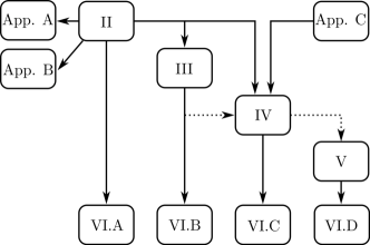
Figure 1: “Roadmap” of the paper with solid (dotted) arrows indicating strong (weak) dependencies.

The following abbreviations are used throughout the text: EP (entropy production), IFP (instantaneous fixed point), ME (master equation), TM (transition matrix), and TSS (time-scale separation).

II Mathematical preliminaries

II.1 Coarse-grained Markov chains

In this section we establish notation and review some known results about Markov processes under coarse-graining. We will start with the description of a discrete, time-homogeneous Markov chain for simplicity, but soon we will move to the physically more relevant case of an arbitrary continuous-time Markov process described by a ME. Finally, we also introduce the concept of lumpability Kemeny and Snell (1976).

Discrete, homogeneous Markov chains.— We consider a Markov process on a discrete space ${\cal{X}}$ with $N$ states $x\in{\cal{X}}$ with a fixed TM $T_{\tau}(x|x^{\prime})$, which propagates the state of the system such that

$$p_{x}(n\tau+\tau)=\sum_{y}T_{\tau}(x|y)p_{y}(n\tau)~{}~{}~{}(n\in\mathbb{N}),$$ (3)

or in vector notation $\textbf{p}(n\tau+\tau)=T_{\tau}\textbf{p}(n\tau)$. Here, $p_{x}(n\tau)$ is the probability to find the system in the state $x$ at time $n\tau$, where $\tau>0$ is an arbitrary but fixed time step (here and in what follows we will set the initial time to ${t_{0}\equiv 0}$). Probability theory demands that $\sum_{x}p_{x}(n\tau)=1$, $p_{x}(n\tau)\geq 0$ for all $x$, $\sum_{x}T_{\tau}(x|y)=1$ and $T_{\tau}(x|y)\geq 0$ for all $x,y$. The steady state of the Markov chain is denoted by $\pi_{x}$ and it is defined via the equation $\boldsymbol{\pi}=T_{\tau}\boldsymbol{\pi}$. In this section we exclude the case of multiple steady states for definiteness, although large parts of the resulting theory can be applied to multiple steady states as well.

Next, we consider a partition $\boldsymbol{\chi}=\{\chi_{1},\dots,\chi_{M}\}$ ($1<M<N$) of the state space such that

$$\bigcup_{\alpha=1}^{M}\chi_{\alpha}={\cal{X}},~{}~{}~{}\chi_{\alpha}\cap\chi_{\beta}=\emptyset\text{ for }\alpha\neq\beta.$$ (4)

In the physics literature this is known as a coarse-graining procedure where different “microstates” $x$ are collected together into a “mesostate” $\alpha$, whereas in the mathematical literature this procedure is usually called lumping. In the following we will use both terminologies interchangeably and we denote a microstate $x$ belonging to the mesostate $\alpha$ by $x_{\alpha}$, i.e., $x_{\alpha}\in\chi_{\alpha}$. The idea is illustrated in Fig. 2. We remark that tracing out the degrees of freedom of some irrelevant system (usually called the “bath”) is a special form of coarse-graining. We will encounter this situation, e.g., in Sec. IV.

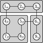
Figure 2: Lumping/coarse-graining of a discrete Markov chain with microstate-space ${\cal{X}}=\{1,2,3,4,5,6,7,8,9\}$ into three mesostates according to the partition $\boldsymbol{\chi}=\{\chi_{\alpha},\chi_{\beta},\chi_{\gamma}\}$ with $\chi_{\alpha}=\{1,2,3\}$, $\chi_{\beta}=\{4,5,7,8\}$ and $\chi_{\gamma}=\{6,9\}$ (grey areas). Possible transistions for which $T_{\tau}(x|y)\neq 0$ are depicted by a solid line connecting state $x$ and $y$.

Any partition $\boldsymbol{\chi}$ defines a stochastic process on the set of mesostates by considering for a given initial distribution $p_{x}(0)$ the probabilities to visit a sequence of mesostates $\alpha,\beta,\gamma,\dots$ at times $0,\tau,2\tau,\dots$ with joint probabilities

$$\begin{split}&p(\beta,\tau;\alpha,0)=\sum_{y_{\beta},x_{\alpha}}T_{\tau}(y_{\beta}|x_{\alpha})p_{x|\alpha}(0)p_{\alpha}(0),\\ &p(\gamma,2\tau;\beta,\tau;\alpha,0)=\\ &\sum_{z_{\gamma},y_{\beta},x_{\alpha}}T_{\tau}(z_{\gamma}|y_{\beta})T_{\tau}(y_{\beta}|x_{\alpha})p_{x|\alpha}(0)p_{\alpha}(0),\end{split}$$ (5)

etc., where $p_{\alpha}(0)=\sum_{x_{\alpha}}p_{x_{\alpha}}(0)$ is the marginalized initial mesostate and $p_{x|\alpha}(0)=p_{x_{\alpha}}(0)/p_{\alpha}(0)$ is the initial microstate conditioned on a certain mesostate $\alpha$. The so generated hierarchy of joint probabilities $p(\alpha_{n},n\tau;\dots;\alpha_{1},\tau;\alpha_{0},0)$ completely specifies the stochastic process at the mesolevel. It is called Markovian whenever the conditional probabilities

$$\begin{split}&p(\alpha_{n},n\tau|\alpha_{n-1},n\tau-\tau;\dots;\alpha_{0},0)\\ &\equiv\frac{p(\alpha_{n},n\tau;\dots;\alpha_{0},0)}{p(\alpha_{n-1},n\tau-\tau;\dots;\alpha_{0},0)}\end{split}$$ (6)

satisfy the Markov property Kemeny and Snell (1976); van Kampen (2007); Rivas et al. (2014); Breuer et al. (2016)

$$\begin{split}&p(\alpha_{n},n\tau|\alpha_{n-1},n\tau-\tau;\dots;\alpha_{0},0)\\ &=p(\alpha_{n},n\tau|\alpha_{n-1},n\tau-\tau).\end{split}$$ (7)

In practice this requires to check infinitely many conditions. But as we will see below, to compute all quantities of thermodynamic interest, only the knowledge about the evolution of the one-time probabilities $p(\alpha_{n},n\tau)$ is important for us.

To see how non-Markovianity affects the evolution of the one time-probabilities, we introduce the following matrices derived from the above joint probabilities

$$G_{\tau,0}(\beta|\alpha) =\frac{p(\beta,\tau;\alpha,0)}{p_{\alpha}(0)}=\sum_{y_{\beta},x_{\alpha}}T_{\tau}(y_{\beta}|x_{\alpha})p_{x|\alpha}(0),$$ (8)

$$\tilde{G}_{2\tau,\tau}(\gamma|\beta) =\frac{p(\gamma,2\tau;\beta,\tau)}{p_{\beta}(\tau)}=\frac{\sum_{\alpha}p(\gamma,2\tau;\beta,\tau;\alpha,0)}{\sum_{\alpha}p(\beta,\tau;\alpha,0)},$$

$$G_{2\tau,0}(\gamma|\alpha) =\frac{p(\gamma,2\tau;\alpha,0)}{p_{\alpha}(0)}$$

$$=\sum_{z_{\gamma},x_{\alpha}}\sum_{\beta,y_{\beta}}T_{\tau}(z_{\gamma}|y_{\beta})T_{\tau}(y_{\beta}|x_{\alpha})p_{x|\alpha}(0).$$

Formally, these matrices are well-defined conditional probabilities because they are positive and normalized. However, we have deliberately choosen a different notation for $\tilde{G}_{2\tau,\tau}$ because only $G_{\tau,0}$ and $G_{2\tau,0}$ can be interpreted as transition probabilities (or matrices) as they generate the correct time evolution for any initial mesostate $p_{\alpha}(0)$. The matrix $\tilde{G}_{2\tau,\tau}$ instead depends on the specific choice of $p_{\alpha}(0)$: if we start with a different initial mesostate $q_{\alpha}(0)\neq p_{\alpha}(0)$, we cannot use $\tilde{G}_{2\tau,\tau}$ to propagate $q_{\beta}(\tau)=\sum_{\beta}G_{\tau,0}(\beta|\alpha)q_{\alpha}(0)$ further in time. This becomes manifest by realizing that the so generated hierarchy of conditional probabilities does not in general obey the Chapman-Kolmogorov equation,

$$G_{2\tau,0}(\gamma|\alpha)=\sum_{\beta}\tilde{G}_{2\tau,\tau}(\gamma|\beta)G_{\tau,0}(\beta|\alpha).$$ (9)

A way to avoid this undesired feature is to define the TM from time $\tau$ to $2\tau$ via the inverse of $G_{\tau,0}$ (provided it exists) Hänggi and Thomas (1977); Rivas et al. (2010, 2014); Breuer et al. (2016)

$$G_{2\tau,\tau}\equiv G_{2\tau,0}G_{\tau,0}^{-1}.$$ (10)

The TM $G_{2\tau,\tau}$ does not depend on the initial mesostate, preserves the normalization of the state and by construction, it fulfills the Chapman-Kolmogorov equation: $G_{2\tau,0}=G_{2\tau,\tau}G_{\tau,0}$. However, as the inverse of a positive matrix is not necessarily positive, $G_{2\tau,\tau}$ can have negative entries. This clearly indicates that $G_{2\tau,\tau}(\gamma|\beta)$ cannot be interpreted as a conditional probability and hence, the process must be non-Markovian. Based on these insights we introduce a weaker notion of Markovianity, which we coin 1-Markovianity. In the context of open quantum systems dynamics this notion is often simply called Markovianity Rivas et al. (2014); Breuer et al. (2016):

Definition II.1 (1-Markovianity).

A stochastic process is said to be 1-Markovian, if the set of TMs $\{G_{n\tau,m\tau}|n\geq m\geq 0\}$ introduced above fulfill $G_{n\tau,m\tau}(\alpha|\beta)\geq 0$ for all $n\geq m\geq 0$ and all $\alpha,\beta$.

It is important to realize that the notion of 1-Markovianity is weaker than the notion of Markovianity: if the coarse-grained process is Markovian, then it is also 1-Markovian and the TMs coincide with the conditional probabilities in Eq. (7). Furthermore, there exist processes which are 1-Markovian but not Markovian according to Eq. (7) (see, e.g., Ref. Rivas et al. (2014)).

Before we consider MEs, we introduce some further notation. We let

$${\cal{A}}(0)\equiv\{p_{x}(0)|p_{\alpha}(0)\text{ arbitrary, }p_{x|\alpha}(0)\text{ fixed}\}$$ (11)

be the set of all physically admissible initial states with respect to a partition $\boldsymbol{\chi}$ (whose dependence is implicit in the notation). The reason to keep $p_{x|\alpha}(0)$ fixed is twofold: first, in an experiment one usually does not have detailed control over the microstates, and second, the TMs (8) for the lumped process depend on $p_{x|\alpha}(0)$, i.e., every choice of $p_{x|\alpha}(0)$ defines a different stochastic process at the mesolevel and should be treated separately. Which of the mesostates $p_{\alpha}(0)$ we can really prepare in an experiment is another interesting (but for us unimportant) question; sometimes this could be only a single state (e.g., the steady state $\pi_{\alpha}$). Of particular importance for the applications later on will be the set

$${\cal{A}}_{\pi}\equiv\{p_{\alpha}\pi_{x|\alpha}|p_{\alpha}\text{ arbitrary}\}$$ (12)

where $\pi_{x|\alpha}=\pi_{x_{\alpha}}/\pi_{\alpha}$ is the conditional steady state. Experimentally, such a class of states can be prepared by holding the mesostate fixed while allowing the microstates to reach steady state. Finally, we define the set of time-evolved admissible initial states

$${\cal{A}}(\tau)\equiv\{\textbf{p}(\tau)=T_{\tau}\textbf{p}(0)|\textbf{p}(0)\in{\cal{A}}(0)\}.$$ (13)

Time-dependent MEs.— For many physical applications it is indeed easier to derive a ME, which describes the continuous time evolution of the system state, compared to deriving a TM for a finite time-step van Kampen (2007); Breuer and Petruccione (2002). The ME reads in general

$$\frac{\partial}{\partial t}p_{x}(t)=\sum_{y}W_{x,y}(\lambda_{t})p_{y}(t)$$ (14)

or in vector notation $\partial_{t}\textbf{p}(t)=W(\lambda_{t})\textbf{p}(t)$. The rate matrix $W(\lambda_{t})$ fulfills $\sum_{x}W_{x,y}(\lambda_{t})=0$ and $W_{x,y}(\lambda_{t})\geq 0$ for $x\neq y$ and it is now also allowed to be parametrically dependent on time through a prescribed parameter $\lambda_{t}$. This situation usually arises by subjecting the system to an external drive, e.g., a time-dependent electric or magnetic field. Furthermore, we assume that the rate matrix has one IFP, which fulfills $W(\lambda_{t})\boldsymbol{\pi}(\lambda_{t})=0$. Clearly, the steady state will in general also parametrically depend on $\lambda_{t}$.

We can connect the ME description to the theory above by noting that the TM over any finite time interval ${[t,t+\tau]}$ is formally given by

$$T_{t,t+\tau}={\cal{T}}_{+}\exp\int_{t}^{t+\tau}W(\lambda_{s})ds,$$ (15)

where ${\cal{T}}_{+}$ is the time-ordering operator. In particular, if we choose $\delta t=\tau/N$ small enough such that $\lambda_{t+\delta t}\approx\lambda_{t}$ (assuming that $\lambda_{t}$ changes continuously in time), we can approximate the TM to any desired accuracy via

$$T_{t+\tau,t}\approx\prod_{i=0}^{N-1}T_{t+i\delta t+\delta t,t+i\delta t}\equiv\prod_{i=0}^{N-1}e^{W(\lambda_{t+i\delta t})\delta t}.$$ (16)

As a notational convention, whenever the system is undriven (i.e., $\dot{\lambda}_{t}=0$ for all $t$), we will simply drop the dependence on $\lambda_{t}$ in the notation.

We now fix an arbitrary partition $\boldsymbol{\chi}$ as before. To describe the dynamics at the mesolevel, one can use several formally exact procedures, two of them we mention here. First, from Eq. (14) we get by direct coarse-graining

$$\begin{split}\frac{\partial}{\partial t}p_{\alpha}(t)&=\sum_{\beta}R_{\alpha,\beta}[\lambda_{t},p_{\alpha}(0)]p_{\beta}(t),\\ R_{\alpha,\beta}[\lambda_{t},p_{\alpha}(0)]&\equiv\sum_{x_{\alpha},y_{\beta}}W_{x_{\alpha},y_{\beta}}(\lambda_{t})p_{y|\beta}(t).\end{split}$$ (17)

Here, the matrix $R[\lambda_{t},p_{\alpha}(0)]$ still fulfills all properties of an ordinary rate matrix: $\sum_{\alpha}R_{\alpha,\beta}[\lambda_{t},p_{\alpha}(0)]=0$ and $R_{\alpha,\beta}[\lambda_{t},p_{\alpha}(0)]\geq 0$ for $\alpha\neq\beta$. However, it explicitly depends on the initial mesostate $p_{\alpha}(0)$, which influences $p_{y|\beta}(t)$ for later times $t$. This is analogous to the problem mentioned below Eq. (8): the TMs computed with Eq. (17) at intermediate times depend on the initial state of the system. This reflects the non-Markovian character of the dynamics and makes it inconvenient for practical applications. Note that Eq. (17) still requires to solve for the full microdynamics and does not provide a closed reduced dynamical description.

A strategy to avoid this undesired feature follows the logic of Eq. (10) and only makes use of the well-defined transition probability [cf. Eq. (8)]

$$G_{t,0}(\alpha|\beta)\equiv\sum_{x_{\alpha},y_{\beta}}T_{t,0}(x_{\alpha}|y_{\beta})p_{y|\beta}(0).$$ (18)

Provided that its inverse exists, it allows to define an effective ME independent of the initial mesostate Hänggi and Thomas (1977); Rivas et al. (2010, 2014); Breuer et al. (2016),

$$\frac{\partial}{\partial t}p_{\alpha}(t) =\sum_{\beta}V_{\alpha,\beta}(\lambda_{t},t)p_{\beta}(t),$$ (19)

$$V(\lambda_{t},t) \equiv\lim_{\delta t\rightarrow 0}\frac{G_{t+\delta t,0}G_{t,0}^{-1}-1}{\delta t},$$ (20)

but where the matrix $V(\lambda_{t},t)$ now carries an additional time-dependence, which does not come from the parameter $\lambda_{t}$. Notice that the construction (20) shares some similarity with the time-convolutionless ME derived from the Nakajima-Zwanzig projection operator formalism, which is another formally exact ME independent of the initial mesostate Fulinski and Kramarczyk (1968); Shibata et al. (1977); Breuer and Petruccione (2002); de Vega and Alonso (2017). The generator $V(\lambda_{t},t)$ preserves normalization and yields to a set of TMs, which fulfill the Chapman-Kolmogorov equation, but it can have temporarily negative rates, i.e., $V_{\alpha,\beta}(\lambda_{t},t)<0$ for $\alpha\neq\beta$ is possible. This is a clear indicator that the dynamics are not 1-Markovian Hall et al. (2014).

Finally, we note that there are also other MEs to describe the reduced state of the dynamics, e.g., the standard Nakajima-Zwanzig equation which is an integro-differential equation Breuer and Petruccione (2002); de Vega and Alonso (2017). This ME is free from the assumption that the inverse of Eq. (18) exists and therefore more general. On the other hand, we will see in Sec. II.2 that we will need the notion of an IFP of the dynamics, which is hard to define for an integro-differential equation.

Lumpability.— In this final part we introduce the concept of lumpability from Sec. 6.3 in Ref. Kemeny and Snell (1976). It will help us to further understand the conditions which ensure Markovianity at the mesolevel and it will be occassionally used in the following. In unison with Ref. Kemeny and Snell (1976) we first introduce the concept for discrete, time-homogeneous Markov chains before we consider MEs again. Furthermore, we emphasize that in the definition below the notion of Markovianity refers to the usual property (7) and not only to the one-time probabilities. Another related weaker concept (known as “weak lumpability”) is treated for the interested reader in Appendix A.

Definition II.2 (Lumpability).

A Markov chain with TM $T_{\tau}$ is lumpable with respect to a partition $\boldsymbol{\chi}$ if for every initial distribution $p_{x}(0)$ the lumped process is a Markov chain with transition probabilities independent of $p_{x}(0)$.

It follows from the definition that a lumpable process for a given TM $T_{\tau}$ and partition $\boldsymbol{\chi}$, is also a lumpable process for all larger times, i.e., for all $T_{n\tau}=(T_{\tau})^{n}$ with $n>1$ and the same partition $\boldsymbol{\chi}$. The following theorem will be useful for us:

Theorem II.1.

A necessary and sufficient condition for a Markov chain to be lumpable with respect to the partition $\boldsymbol{\chi}$ is that

$${\cal{G}}_{\tau}(\alpha|\beta)\equiv\sum_{x_{\alpha}}T_{\tau}(x_{\alpha}|y_{\beta})=\sum_{x_{\alpha}}T_{\tau}(x_{\alpha}|y^{\prime}_{\beta})$$ (21)

holds for any $y_{\beta}\neq y^{\prime}_{\beta}$. The lumped process then has the TM ${\cal{G}}_{\tau}$.

The details of the proof can be found in Ref. Kemeny and Snell (1976). However, it is obvious that the so-defined set of TMs is independent of the inital state. In addition, one can readily check that they fulfill the Chapman-Kolmogorov equation, are normalized and have positive entries.

The concept of lumpability can be straightforwardly extended to time-dependent MEs by demanding that a lumpable ME with respect to the partition $\boldsymbol{\chi}$ has lumpable TMs $T_{t+\delta t,t}$ for any time $t$ and every $\delta t>0$. By expanding Eq. (21) in $\delta t$ and by taking $\delta t\rightarrow 0$, we obtain the following corollary (see also Ref. Nicolis (2011)):

Corollary II.1.

A ME with possibly time-dependent rates is lumpable with respect to the partition $\boldsymbol{\chi}$ if and only if

$${\cal{V}}_{\alpha,\beta}(\lambda_{t})\equiv\sum_{x_{\alpha}}W_{x_{\alpha},y_{\beta}}(\lambda_{t})=\sum_{x_{\alpha}}W_{x_{\alpha},y^{\prime}_{\beta}}(\lambda_{t})$$ (22)

for any $y_{\beta}\neq y^{\prime}_{\beta}$ and any $t$. The lumped process is then governed by the rate matrix ${\cal{V}}(\lambda_{t})$.

Notice that the dynamical description of a lumpable ME is unambiguous because the generator $R[\lambda_{t},p_{\alpha}(0)]$ from Eq. (17) and $V(\lambda_{t},t)$ from Eq. (20) both coincide with ${\cal{V}}(\lambda_{t})$ from the above corollary. For $R[\lambda_{t},p_{\alpha}(0)]$ this follows from directly applying Eq. (22) to Eq. (17). For $V(\lambda_{t},t)$ this follows from the fact that the propagator in Eq. (10) coincides for a Markovian process with the transition probabilities obtained from Eq. (7), which for a lumpable process are identical to the TMs introduced in Theorem II.1. All generators are then identical and have the same well-defined rate matrix.

In the following we will stop repeating that any concept at the coarse-grained level is always introduced “with respect to the partition $\boldsymbol{\chi}$”. Furthermore, to facilitate the readability, Table 1 summarizes the most important notation used in this section and in the remainder.

symbol	meaning
${\cal{X}}$	full state space
$\boldsymbol{\chi}$	state space partition
$x$	arbitary microstate
$\alpha$	mesostate
$x_{\alpha}$	microstate belonging to mesostate $\alpha$
$\pi_{x}(\lambda_{t})$	microlevel IFP
$\pi_{\alpha}(\lambda_{t})$	$=\sum_{x_{\alpha}}\pi_{x_{\alpha}}(\lambda_{t})$ (no IFP in general!)
${\cal{A}}(0)$	set of admissible initial states
${\cal{A}}_{\pi}(\lambda_{t})$	$\rightarrow$ Eq. (12), in general dependent on $\lambda_{t}$
${\cal{A}}(t)$	${\cal{A}}(0)$ time-evolved
$p_{x}(t)$ [$\rho(x;t)$]	microstate probability discrete [continuous]
$p_{\alpha}(t)$ [$\rho(\alpha;t)$]	mesostate probability discrete [continuous]
$W(\lambda_{t})$	rate matrix for microdynamics
$D[p_{x}\|q_{x}]$	relative entropy

Table 1: List of symbols frequently used in the text.

II.2 Entropy production rates, non-Markovianity and instantaneous fixed points

After having discussed how to describe the dynamics at the mesolevel, we now turn to its thermodynamics. This is still done in an abstract way without recourse to an underlying physical model. An important concept in our theory is the notion of an IFP, which we define as follows:

Definition II.3 (Instantaneous fixed point).

Let $V(\lambda_{t},t)$ be the generator of the time-local ME (19). We say that $\tilde{\boldsymbol{\pi}}(t)$ is an IFP of the dynamics if $V(\lambda_{t},t)\tilde{\boldsymbol{\pi}}(t)=0$.

We notice that $\tilde{\boldsymbol{\pi}}(t)$ does not need to be a well-defined probability distribution because $V(\lambda_{t},t)$ can have negative rates. We also point out that the IFP at time $t$ might not be reachable from any state in the class of initially admissible states and it is therefore a purely abstract concept. Hence, while $V(\lambda_{t},t)\tilde{\boldsymbol{\pi}}(t)=0$ it need not be true that $R[\lambda_{t},p_{\alpha}(0)]\tilde{\boldsymbol{\pi}}(t)=0$ for any $p_{x_{\alpha}}(0)\in{\cal{A}}(0)$. The IFP cannot be computed with the help of the effective rate matrix in Eq. (17). The IFP is only well-defined for a time-local ME with a generator independent of the initial mesostate. In Appendix B we will show that it also does not matter how we have derived the ME as long as it is time-local, formally exact and independent of the initial mesostate.

In the first part of this section, we introduce the concept of EP rate in a formal way and establish a general theorem. In the second part of this section, we will answer the question when does the IFP $\tilde{\boldsymbol{\pi}}(t)$ coincide with the marginalized IFP of the microdynamics,

$$\pi_{\alpha}(\lambda_{t})=\sum_{x_{\alpha}}\pi_{x_{\alpha}}(\lambda_{t}).$$ (23)

EP rate.— We define the EP rate for the coarse-grained process by

$$\begin{split}\dot{\Sigma}(t)&\equiv-\left.\frac{\partial}{\partial t}\right|_{\lambda_{t}}D[p_{\alpha}(t)\|\pi_{\alpha}(\lambda_{t})]\\ &=-\sum_{\alpha}\frac{\partial p_{\alpha}(t)}{\partial t}[\ln p_{\alpha}(t)-\ln\pi_{\alpha}(\lambda_{t})],\end{split}$$ (24)

where $\pi_{\alpha}(\lambda_{t})$ was defined in Eq. (23). Notice that $\dot{\Sigma}(t)$ can be defined for any stochastic process and a priori it is not related to the physical EP rate known from nonequilibrium thermodynamics. However, for the systems considered in Secs. III and IV this will turn out to be the case. Having emphasized this point, we decided for simplicity to refrain from introducing a new terminology for $\dot{\Sigma}(t)$ in this section. Furthermore, we remark that the definition of $\dot{\Sigma}(t)$ is experimentally meaningful: it only requires to measure the mesostate $p_{\alpha}(t)$ and the knowledge of $\pi_{\alpha}(\lambda_{t})$. The latter can be obtained by measuring the steady state of the system after holding $\lambda_{t}$ fixed for a long time or by arguments of equilibrium statistical mechanics (see Secs. III and IV). Also theoretically, Eq. (24) can be evaluated with any method that gives the exact evolution of the mesostates.

The following theorem shows how to connect negative EP rates to non-Markovianity. Application of this theorem to various physical situations will be the purpose of the next sections.

Theorem II.2.

If $\pi_{\alpha}(\lambda_{t})$ is an IFP of the mesodynamics and if $I$ denotes the time interval in which the mesodynamics are 1-Markovian, then $\dot{\Sigma}(t)\geq 0$ for all $t\in I$.

To prove this theorem, it is useful to recall the well-known lemma, which we have stated already in Eq. (1):

Lemma II.1.

For a 1-Markovian process the relative entropy between any two probability distributions is continuously decreasing in time, i.e., for all $t$ and any pair of intial distributions $p_{\alpha}(0)$ and $q_{\alpha}(0)$ Eq. (1) holds.

This lemma follows from the fact that, firstly, for every stochastic matrix $M$ and any pair of distributions $p_{\alpha}$ and $q_{\alpha}$ one has that

$$D\left[\sum_{\beta}M_{\alpha,\beta}p_{\beta}\left\|\sum_{\beta}M_{\alpha,\beta}q_{\beta}\right]\right.\leq D[p_{\alpha}\|q_{\alpha}],$$ (25)

and secondly, for a 1-Markovian process the TM at any time $t$ and for every time step $\delta t$ is stochastic. We can now prove Theorem II.2:

Proof.

By definition of the EP rate we have

$$\dot{\Sigma}(t)=$$ (26)

$$-\lim_{\delta t\rightarrow 0}\frac{D[G_{t+\delta t,t}\textbf{p}_{\text{cg}}(t)\|\boldsymbol{\pi}_{\text{cg}}(\lambda_{t})]-D[\textbf{p}_{\text{cg}}(t)\|\boldsymbol{\pi}_{\text{cg}}(\lambda_{t})]}{\delta t},$$

where $G_{t+\delta t,t}$ is the propagator obtained from the ME (19) [cf. also Eq. (10)], $\textbf{p}_{\text{cg}}(t)$ denotes the vector of the coarse-grained state $p_{\alpha}(t)$ and likewise for $\boldsymbol{\pi}_{\text{cg}}(\lambda_{t})$. Next, we use the assumption that $\boldsymbol{\pi}_{\text{cg}}(\lambda_{t})$ is an IFP of the ME (19), i.e., we have

$$G_{t+\delta t,t}\boldsymbol{\pi}_{\text{cg}}(\lambda_{t})\approx\boldsymbol{\pi}_{\text{cg}}(\lambda_{t})$$ (27)

and any possible discrepancy vanishs in the limit $\delta t\rightarrow 0$. Thus, we can rewrite Eq. (26)

$$\begin{split}\dot{\Sigma}(t)=-\lim_{\delta t\rightarrow 0}\frac{1}{\delta t}\big{\{}&D[G_{t+\delta t,t}\textbf{p}_{\text{cg}}(t)\|G_{t+\delta t,t}\boldsymbol{\pi}_{\text{cg}}(\lambda_{t})]\\ &-D[\textbf{p}_{\text{cg}}(t)\|\boldsymbol{\pi}_{\text{cg}}(\lambda_{t})]\big{\}}.\end{split}$$ (28)

Now, if the dynamics is 1-Markovian (Definition II.1), then $G_{t+\delta t,t}$ is a stochastic matrix and from Eq. (25) it follows that $\dot{\Sigma}(t)\geq 0$. ∎

Whereas the proof of Theorem II.2 is straightforward, two things make it a non-trivial statement. First, we will show that the EP rate defined in Eq. (24) deserves its name because it can be linked to physical quantities with a precise thermodynamic interpretation. This will be done in Secs. III and IV. Second, the essential assumption that $\pi_{\alpha}(\lambda_{t})$ is an IFP of the mesodynamics is non-trivial: it is not a consequence of a 1-Markovian time-evolution and it can also happen for non-Markovian dynamics. The details of this crucial assumption will be worked out in the remainder of this section, but already at this point we emphasize that 1-Markovianity alone is not sufficient to guarantee that $\dot{\Sigma}(t)\geq 0$. The Venn diagramm in Fig. 3 should help to understand the implications of Theorem II.2 better.

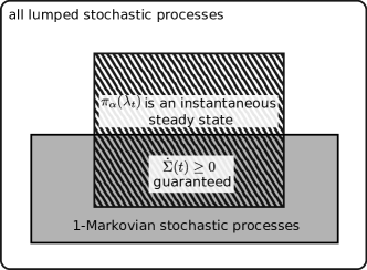
Figure 3: A Venn-diagramm to understand the implications of Theorem II.2. The largest outer box contains all possible lumped stochastic process. One subset of them is 1-Markovian (shaded in grey). For another subset the maginalized microlevel steady state $\pi_{\alpha}(\lambda_{t})$ is an IFP of the dynamics (striped area). Where both sets overlap, $\dot{\Sigma}(t)\geq 0$ is guaranteed, i.e., whenever we observe $\dot{\Sigma}(t)<0$ we cannot be simultaneously in the striped and in the shaded grey area. Note that the Venn-diagramm shows the situation for a fixed driving protocol $\lambda_{t}$ and time interval $I$. Depending on $\lambda_{t}$ and $I$ the shaded grey and the striped area can parametrically change in time.

IFP of the coarse-grained process.— To answer the question when is $\tilde{\pi}_{\alpha}(\lambda_{t})=\pi_{\alpha}(t)$, we start with the simple case and assume that the coarse-grained dynamics are lumpable. Hence, according to Corollary II.1 there is a unique and well-defined rate matrix. We then get:

Theorem II.3.

If the stochastic process is lumpable for some time interval $I$, then the IFP of the mesostates is given by the marginal IFP of $W(\lambda_{t})$ for all $t\in I$.

Proof.

We want to show that ${\cal{V}}(\lambda_{t})\boldsymbol{\pi}(\lambda_{t})=0$. By using Corollary II.1 in the first and third equality, we obtain

$$\begin{split}\sum_{\beta}{\cal{V}}_{\alpha,\beta}(\lambda_{t})\pi_{\beta}(\lambda_{t})&=\sum_{\beta}\sum_{x_{\alpha}}W_{x_{\alpha},y_{\beta}}(\lambda_{t})\pi_{\beta}(\lambda_{t})\\ &=\sum_{\beta}\sum_{x_{\alpha},y^{\prime}_{\beta}}W_{x_{\alpha},y_{\beta}}(\lambda_{t})\pi_{y^{\prime}_{\beta}}(\lambda_{t})\\ &=\sum_{\beta}\sum_{x_{\alpha},y^{\prime}_{\beta}}W_{x_{\alpha},y^{\prime}_{\beta}}(\lambda_{t})\pi_{y^{\prime}_{\beta}}(\lambda_{t}),\end{split}$$ (29)

which is zero since $\pi_{y^{\prime}_{\beta}}(\lambda_{t})$ is the IFP at the microlevel. ∎

Therefore, together with Theorem II.2 we can infer that $\dot{\Sigma}(t)<0$ unambiguously shows that the dynamics are not lumpable. However, lumpability required the coarse-grained process to fulfill the Markov property (7) for any initial condition, which is a rather strong property. We are therefore interested whether a negative EP rate reveals also insights about the weaker property of 1-Markovianity. For instance, for undriven processes we intuitively expect that, provided that we start at steady state, we always remain at steady state independently of the time-dependence of the generator (20) or even the question whether the inverse of Eq. (18) exists. Then, negative values of the EP rate will always indicate non-Markovian dynamics for undriven system. Indeed, the following theorem holds:

Theorem II.4.

Consider an undriven stochastic process described by the ME (19), i.e., we assume $G_{t,0}^{-1}$ to exist for all admissible initial states ${\cal{A}}(0)$ and all times $t$. If the conditional microstates are initially equilibrated, ${\cal{A}}(0)\subset{\cal{A}}_{\pi}$ [Eq. (12)], then $\pi_{\alpha}$ is an IFP of the stochastic process at the mesolevel.

Proof.

If ${\cal{A}}(0)\subset{\cal{A}}_{\pi}$, we can conclude that $\sum_{\beta}G_{t,0}(\alpha|\beta)\pi_{\beta}=\pi_{\alpha}$, i.e., if we start with the coarse-grained steady state we also remain in it for all times $t$. Since $G_{t,0}$ was assumed to be invertible,

$$\sum_{\beta}(G_{t,0}^{-1})_{\alpha,\beta}\pi_{\beta}=\pi_{\alpha}.$$ (30)

Hence, by definition (20) we obtain the chain of equalities

$$\begin{split}&\sum_{\alpha,\beta}\left(\lim_{\delta t\rightarrow 0}\frac{G_{t+\delta t,0}G_{t,0}^{-1}-1}{\delta t}\right)_{\alpha,\beta}\pi_{\beta}\\ &=\lim_{\delta t\rightarrow 0}\frac{1}{\delta t}\left[\sum_{\beta,\gamma}G_{t+\delta t,0}(\alpha|\gamma)(G_{t,0}^{-1})_{\gamma,\beta}\pi_{\beta}-\pi_{\alpha}\right]\\ &=\lim_{\delta t\rightarrow 0}\frac{1}{\delta t}\left[\sum_{\gamma}G_{t+\delta t,0}(\alpha|\gamma)\pi_{\gamma}-\pi_{\alpha}\right]\\ &=\lim_{\delta t\rightarrow 0}\frac{1}{\delta t}\left[\pi_{\alpha}-\pi_{\alpha}\right]=0.\end{split}$$ (31)

∎

We recognize a big difference in the characterization of the IFPs for driven and undriven processes. Without driving, the right set of initial states suffices already to show that the microlevel steady state induces the steady state at the mesolevel, even if the dynamics is non-Markovian. Thus, for this kind of dynamics $\dot{\Sigma}(t)<0$ unambiguously signifies non-Markovianity. For driven systems instead, we needed the much stronger requirement of lumpability, i.e., Markovianity of the lumped process with TMs independent of the initial microstate. However, at least formally it is possible to establish the following additional theorem:

Theorem II.5.

Consider a driven stochastic process described by the ME (19), i.e., we assume $G_{t,0}^{-1}$ to exist for all initial states and all times $t$. We denote by $I$ the time-interval in which either

1. all conditional microstates in the set of time-evolved states are at steady state, ${\cal{A}}(t)\subset{\cal{A}}_{\pi}(\lambda_{t})$, or

2. the IFP of the microdynamics is an admissible time-evolved state, $\pi_{x}(\lambda_{t})\in{\cal{A}}(t)$.

Then, $\pi_{\alpha}(\lambda_{t})$ is an IFP of the lumped process for all $t\in I$.

Proof.

First of all, notice that the ME (19) generates the exact time evolution, i.e., for any $p_{y}(t)=p_{\beta}(t)p_{y|\beta}(t)\in{\cal{A}}(t)$ we have

$$\begin{split}&\sum_{\beta}V_{\alpha,\beta}(\lambda_{t},t)p_{\beta}(t)\\ &=\sum_{x_{\alpha}}\sum_{\beta,y_{\beta}}W_{x_{\alpha},y_{\beta}}(\lambda_{t})p_{y|\beta}(t)p_{\beta}(t).\end{split}$$ (32)

For the first condition, if $\pi_{x}(\lambda_{t})\in{\cal{A}}(t)\subset{\cal{A}}_{\pi}(\lambda_{t})$, then one immediately verifies that $V(\lambda_{t},t)\boldsymbol{\pi}(\lambda_{t})=0$. But one may have that ${\cal{A}}(t)\subset{\cal{A}}_{\pi}(\lambda_{t})$, but $\pi_{x}(\lambda_{t})\notin{\cal{A}}(t)$. This means that there is no admissible initial state, which gets mapped to the IFP at time $t$, i.e., $T_{t,0}^{-1}\boldsymbol{\pi}(\lambda_{t})\notin{\cal{A}}(0)$. However, by the invertibility of the dynamics there is always a set of states $p_{x}^{(i)}(t)\in{\cal{A}}(t)$, which spans the entire mesostate space. Thus, we can always find a linear combination $\pi_{x}(\lambda_{t})=\sum_{i}\mu_{i}p_{x}^{(i)}(t)$ with $\mu_{i}\in\mathbb{R}$. Then, $V(\lambda_{t},t)\boldsymbol{\pi}(\lambda_{t})=0$ follows from the linearity of the dynamics by applying Eq. (LABEL:eq_help_4) to each term of the linear combination.

For the second condition let us assume the opposite, i.e., $V(\lambda_{t},t)\boldsymbol{\pi}(\lambda_{t})\neq 0$. This implies $\sum_{\beta}G_{t+\delta t,t}(\alpha|\beta)\pi_{\beta}(\lambda_{t})\neq\pi_{\alpha}(\lambda_{t})$ for a sufficiently small $\delta t$. But as the reduced dynamics are exact, this can only be the case if there is a state $q_{y}(t)=\pi_{\beta}(\lambda_{t})q_{y|\beta}(t)\in{\cal{A}}(t)$ with $q_{y|\beta}(t)\neq\pi_{y|\beta}(\lambda_{t})$. On the other hand, the theorem assumes that $\pi_{x}(\lambda_{t})\in{\cal{A}}(t)$ too. Hence, there must be two states $q_{y}(t)\in{\cal{A}}(t)$ and $\pi_{x}(\lambda_{t})\in{\cal{A}}(t)$, which give the same marginal mesostate $\pi_{\alpha}(\lambda_{t})$. Since the ME dynamics in the full space are clearly invertible and since the initial conditional microstate is fixed, this means that there must be two different initial mesostates, which get mapped to the same mesostate at time $t$. Hence, $G_{t,0}$ cannot be invertible, which conflicts with our initial assumption. ∎

Theorem II.5 plays an important role in the limit of TSS (see Sec. III.3) where the first condition is automatically fulfilled. The second condition will be in general complicated to check if the microdynamics are complex.

It is worthwhile to ask whether milder conditions suffice to ensure that $\pi_{\alpha}(\lambda_{t})$ is an IFP of the mesodynamics. In Appendix A we show that they can indeed be found if the dynamics fulfills the special property of weak lumpability. In general, however, we believe that it will be hard to find milder conditons: in Sec. VI.1 we give an example for an ergodic and undriven Markov chain, whose mesodynamics are 1-Markovian, but $\pi_{\alpha}$ is not an IFP unless ${\cal{A}}(0)\subset{\cal{A}}_{\pi}$. As any driven process takes the conditional microstates out of equilibrium, i.e., ${\cal{A}}(t)\nsubseteq{\cal{A}}_{\pi}(\lambda_{t})$ in general, finding useful milder conditions to guarantee that $\pi_{\alpha}(\lambda_{t})$ is an IFP seems unrealistic.

Before we proceed with the physical picture, we want to comment on a mathematical subtlety, which becomes relevant for the application considered in Sec. IV. In there, we will apply our findings from above to the case of Hamiltonian dynamics described on the continuous phase space of a collection of classical particles. This does not fit into the conventional picture of a finite and discrete state space ${\cal{X}}$ with $N<\infty$ microstates. However, under the assumption that it is possible to approximate the actual Hamiltonian dynamics by using a high-dimensional grid of very small phase space cells, we can imagine that we can approximate the true dynamics arbitrarily well with a finite, discretized phase space. Nevertheless, in order not to rely on this way of reasoning, we briefly re-derive the above theorems for the Hamiltonian setting in Appendix C.

III Coarse-grained dissipative dynamics

III.1 Thermodynamics at the microlevel

We now start to investigate the first application of the general framework from Sec. II. In this section we consider the ME (14), which describes a large class of dissipative classical and quantum systems, with applications ranging from molecular motors to thermoelectric devices. In addition, we impose the condition of local detailed balance,

$$\ln\frac{W_{x,y}(\lambda_{t})}{W_{y,x}(\lambda_{t})}=-\beta[E_{x}(\lambda_{t})-E_{y}(\lambda_{t})],$$ (33)

where $E_{x}(\lambda_{t})$ denotes the energy of state $x$ and $\beta$ the inverse temperature of the bath. Eq. (33) ensures that the IFP at the microlevel is given by the Gibbs state $\pi_{x}(\lambda_{t})=e^{-\beta E_{x}(\lambda_{t})}/Z(\lambda_{t})$ with $Z(\lambda_{t})=\sum_{x}e^{-\beta E_{x}(\lambda_{t})}$ and it allows us to link energetic changes in the system with entropic changes in the bath. A thermodynamically consistent description of the microdynamics follows from the definitions

$$U_{\text{mic}}(t) \equiv\sum_{x}E_{x}(\lambda_{t})p_{x}(t)~{}(\text{internal energy}),$$ (34)

$$\dot{W}_{\text{mic}}(t) \equiv\sum_{x}[d_{t}E_{x}(\lambda_{t})]p_{x}(t)~{}(\text{work rate}),$$ (35)

$$\dot{Q}_{\text{mic}}(t) \equiv\sum_{x}E_{x}(\lambda_{t})\partial_{t}p_{x}(t)~{}(\text{heat rate}),$$ (36)

$$S_{\text{mic}}(t) \equiv-\sum_{x}p_{x}(t)\ln p_{x}(t)~{}(\text{Shannon entropy}),$$ (37)

$$F_{\text{mic}}(t) \equiv U_{\text{mic}}(t)-S_{\text{mic}}(t)/\beta~{}(\text{free energy}),$$ (38)

$$\dot{\Sigma}_{\text{mic}}(t) \equiv-\left.\frac{\partial}{\partial t}\right|_{\lambda_{t}}D[p_{x}(t)\|\pi_{x}(\lambda_{t})]\geq 0~{}(\text{EP rate}).$$ (39)

Here, we used the subscript “mic” to emphasize that the above definitions refer to the thermodynamic description of the microdynamics, which has to be distinguished from the thermodynamic description at the mesolevel introduced below. Using the ME (14) and local detailed balance (33) together with the definitions provided above, one can verify the first and second law of thermodynamics in the conventional form: $d_{t}U_{\text{mic}}(t)=\dot{W}_{\text{mic}}(t)+\dot{Q}_{\text{mic}}(t)$ and $\dot{\Sigma}_{\text{mic}}(t)=\beta[\dot{W}_{\text{mic}}(t)-d_{t}F_{\text{mic}}(t)]\geq 0$.

Since the IFP at the microlevel is the equilibrium Gibbs state, we can parametrize the conditional equilibrium state of the microstates belonging to a mesostate $\alpha$ as

$$\pi_{x|\alpha}(\lambda_{t})=e^{-\beta[E_{x_{\alpha}}(\lambda_{t})-F_{\alpha}(\lambda_{t})]},$$ (40)

where $F_{\alpha}(\lambda_{t})\equiv-\beta^{-1}\ln\sum_{x_{\alpha}}e^{-\beta E_{x_{\alpha}}(\lambda_{t})}$ plays the role of an effective free energy. The reduced equilibrium distribution of a mesostate can then be written as

$$\pi_{\alpha}(\lambda_{t})=\frac{e^{-\beta F_{\alpha}(\lambda_{t})}}{Z(\lambda_{t})}.$$ (41)

In the following we want to find meaningful definitions, which allow us to formulate the laws of thermodynamics at a coarse-grained level and which we can connect to the general theory of Sec. II. Since the dynamics at the mesolevel will typically be non-Markovian and not fulfill local detailed balance, finding a consistent thermodynamic framework becomes non-trivial. We will restrict our investigations here to any initial prepartion class which fulfills ${\cal{A}}(0)\subset{\cal{A}}_{\pi}(\lambda_{0})$ with ${\cal{A}}_{\pi}(\lambda_{0})$ defined in Eq. (12). If the dynamics is driven, we will need one additional assumption [see Eq. (42)], otherwise our results are general.

III.2 Thermodynamics at the mesolevel

With the framework from Sec. II we are now going to study the thermodynamics at the mesolevel. This is possible in full generality if the dynamics are undriven. In case of driving, $\dot{\lambda}_{t}\neq 0$, we need to assume that we can split the time-dependent energy function as

$$E_{x_{\alpha}}(\lambda_{t})=E_{\alpha}(\lambda_{t})+\tilde{E}_{x_{\alpha}}.$$ (42)

Thus, solely the mesostate energies are affected by the driving. This condition naturally arises if we think about the complete system as being composed of two interacting systems, ${\cal{X}}={\cal{Y}}\otimes{\cal{Z}}$, and we trace out the degrees of freedom ${\cal{Y}}$ to obtain a reduced description in ${\cal{Z}}$. In this case we can split the energy for any value of $\lambda_{t}$ as $E_{yz}=E_{y}+E_{z}+V_{yz}$ where $V_{yz}$ describes an interaction energy and $E_{y}$ ($E_{z}$) are the bare energies associated with the isolated system ${\cal{Y}}$ (${\cal{Z}}$). Condition (42) is then naturally fulfilled if we identify $E_{z}=E_{\alpha}$ and only $E_{z}=E_{z}(\lambda_{t})$ is time-dependent (compare also with Sec. IV). Importantly, this condition allows us to identify

$$\begin{split}\dot{W}_{\text{mic}}(t)&=\sum_{x}\frac{\partial E_{x}(\lambda_{t})}{\partial t}p_{x}(t)\\ &=\sum_{\alpha}\frac{\partial E_{\alpha}(\lambda_{t})}{\partial t}p_{\alpha}(t)\equiv\dot{W}(t).\end{split}$$ (43)

Therefore, the exact rate of work can be computed from the knowledge about the mesostate alone. Furthermore, Eq. (42) implies that the conditional equilibrium state of the bath (40) does not depend on $\lambda_{t}$ and hence, we can write ${\cal{A}}_{\pi}(\lambda_{0})={\cal{A}}_{\pi}$.

The thermodynamic analysis starts from our central definition (24)

$$\dot{\Sigma}(t)=-\left.\frac{\partial}{\partial t}\right|_{\lambda_{t}}D[p_{\alpha}(t)\|\pi_{\alpha}(\lambda_{t})]$$ (44)

with $\pi_{\alpha}(\lambda_{t})$ given in Eq. (41). Using Eq. (43) and noting that $d_{t}F_{\alpha}(\lambda_{t})=d_{t}E_{\alpha}(\lambda_{t})$, it is not hard to confirm that

$$\dot{\Sigma}(t)=\beta\dot{W}(t)-\beta\frac{d}{dt}\sum_{\alpha}p_{\alpha}(t)\left[F_{\alpha}(\lambda_{t})+\frac{1}{\beta}\ln p_{\alpha}(t)\right].$$ (45)

This motivates the definition of the nonequilibrium free energy

$$F(t)\equiv\sum_{\alpha}p_{\alpha}(t)\left[F_{\alpha}(\lambda_{t})+\frac{1}{\beta}\ln p_{\alpha}(t)\right],$$ (46)

such that the EP rate is given by the familiar form of phenomenological non-equilibrium thermodynamics: $\dot{\Sigma}(t)=\beta[\dot{W}(t)-d_{t}F(t)]$. The EP over a finite time interval becomes

$$\Sigma(t)=\beta[W(t)-\Delta F(t)]$$ (47)

and for a proper second law it remains to show that this quantity is positive. This follows from:

Theorem III.1.

For any $p_{x}(0)\in{\cal{A}}_{\pi}$ and any driving protocol we have

$$\Sigma(t)\geq\Sigma_{\text{mic}}(t)\geq 0.$$ (48)

Proof.

The proof was already given in Ref. Strasberg and Esposito (2017). In short, one rewrites

$$\Sigma(t)-\Sigma_{\text{mic}}(t)=\beta[\Delta F_{\text{mic}}(t)-\Delta F(t)]$$ (49)

and shows that for $p_{x}(0)\in{\cal{A}}_{\pi}$ it follows that

$$\begin{split}&\beta[\Delta F_{\text{mic}}(t)-\Delta F(t)]\\ &=D[p_{x}(t)\|\pi_{x}(\lambda_{t})]-D[p_{\alpha}(t)\|\pi_{\alpha}(\lambda_{t})]\\ &=\sum_{\alpha}p_{\alpha}(t)D[p_{x|\alpha}(t)\|\pi_{x|\alpha}]\geq 0.\end{split}$$ (50)

Since $\Sigma_{\text{mic}}(t)\geq 0$, this implies $\Sigma(t)\geq 0$. ∎

Using the theorems of Sec. II.2, we can now connect the appearance of negative EP rates to the following properties of the underlying dynamics:

Theorem III.2.

Let $p_{x}(0)\in{\cal{A}}_{\pi}$ and let $I$ denote the time interval in which the mesodynamics are 1-Markovian and the dynamics is

1. undriven, or

2. driven and lumpable, or

3. driven and such that ${\cal{A}}(t)\subset{\cal{A}}_{\pi}$ or $\pi_{x}(\lambda_{t})\in{\cal{A}}(t)$.

Then, $\dot{\Sigma}(t)\geq 0$ for all $t\in I$ and all admissible initial states.

Hence, as a corollary, if we observe $\dot{\Sigma}(t)<0$ for the undriven case, we know that the dynamics is non-Markovian [or that the initial state $p_{x}(0)\notin{\cal{A}}_{\pi}$]. For driven dynamics, noticing a negative EP rate, is not sufficient to conclude that the dynamics is non-Markovian, but they are clearly not lumpable. In the next section we will show that $\dot{\Sigma}(t)<0$ also suffices to conlude that TSS does not apply.

Furthermore, while the above procedure provides a unique way to define a non-equilibrium free energy at the mesolevel, it does not fix the definition of the internal energy and entropy at the mesolevel because the prescription $F=U-S/\beta$ entails a certain level of arbitrariness. Via the first law $\Delta U=Q+W$ this would also imply a certain arbitrariness for the definition of heat Talkner and Hänggi (2016). However, a reasonable definition of $U,S$ and $Q$ can be fixed by demanding that they should coincide with $U_{\text{mic}},S_{\text{mic}}$ and $Q_{\text{mic}}$ in the limit where the microstates are conditionally equilibrated, which is fulfilled in the limit of TSS considered in Sec. III.3. Then, one is naturally lead to the definitions

$$U(t) \equiv\sum_{\alpha}{\cal{U}}_{\alpha}(\lambda_{t})p_{\alpha}(t),~{}~{}~{}{\cal{U}}_{\alpha}\equiv\sum_{x_{\alpha}}E_{x_{\alpha}}(\lambda_{t})\pi_{x|\alpha},$$ (51)

$$S(t) \equiv\sum_{\alpha}\left\{\beta[{\cal{U}}_{\alpha}(\lambda_{t})-F_{\alpha}(\lambda_{t})]-\ln p_{\alpha}(t)\right\}p_{\alpha}(t).$$ (52)

Heat is then defined as $\dot{Q}(t)=d_{t}U(t)-\dot{W}(t)$ and the EP rate can be equivalently expressed as $\dot{\Sigma}(t)=d_{t}S(t)-\beta\dot{Q}(t)$.

We remark that it is not obvious how to relax condition (42) because the work (43) can then not be computed from knowledge of the mesostate alone, which was an essential ingredient in our derivation.

III.3 Time-scale separation and Markovian limits

Although open systems behave non-Markovian in general, it is important to know in which limits the Markovian approximation is justified. One such limit is TSS, which is an essential assumption in many branches of statistical mechanics in order to ensure that the dynamics at the level of the “relevant” degrees of freedom is Markovian and hence, easily tractable. It is also essential in order to ensure that we can infer from the coarse-grained dynamics the exact thermodynamics of the underlying microstate dynamics (under reasonable mild conditions), see Refs. Puglisi et al. (2010); Seifert (2011); Esposito (2012); Altaner and Vollmer (2012); Bo and Celani (2014); Strasberg and Esposito (2017) for research on this topic. Here, we restrict ourselves to highlight the role of TSS within our mathematical framework of Sec. II. Furthermore, at the end of this section we discuss another class of systems whose dynamics is Markovian albeit TSS does not apply.

To study TSS, let us decompose the rate matrix as follows:

$$W_{x_{\alpha},y_{\beta}}(\lambda_{t})=\delta_{\alpha\beta}R_{x_{\alpha},y_{\alpha}}(\lambda_{t})+(1-\delta_{\alpha\beta})r_{x_{\alpha},y_{\beta}}(\lambda_{t}).$$ (53)

Next, we assume that $R_{x_{\alpha},y_{\alpha}}(\lambda_{t})\gg r_{x_{\alpha},y_{\beta}}(\lambda_{t})$, i.e., there is a strong separation of time-scales between the mesodynamics and the microdynamics belonging to a certain mesostate. As a consequence the microstates rapidly equilibrate to the conditional steady state $\pi_{x|\alpha}(\lambda_{t})$ for any mesostate $\alpha$ provided that the microstates in each mesostate are fully connected (tacitly assumed in the following). This means that condition 1 of Theorem II.5 is always fulfilled. By replacing $p_{y|\beta}(t)$ by $\pi_{y|\beta}(\lambda_{t})$ in Eq. (17), it is easy to see that the effective rate matrix is independent of the initial state and describes a proper Markov process, $R[\lambda_{t},p_{\alpha}(0)]=R(\lambda_{t})$. Another consequence of TSS is that the thermodynamics associated with the mesodynamics are identical to the thermodynamics of the microdynamics.

Strictly speaking the limit of TSS requires $R_{x_{\alpha},y_{\alpha}}(\lambda_{t})/r_{x_{\alpha},y_{\beta}}(\lambda_{t})\rightarrow\infty$. In practice, however, there will be always a finite time $\delta t$ associated with the relaxation of the microstates and TSS means that we assume

$$\frac{1}{r_{x_{\alpha},y_{\beta}}(\lambda_{t})}\gg\delta t\gg\frac{1}{R_{x_{\alpha},y_{\alpha}}(\lambda_{t})}.$$ (54)

Then, within a time-step $\delta t$ the conditional microstates are almost equilibrated while terms of the order ${\cal{O}}(\delta t^{2}r_{x_{\alpha},y_{\beta}})$ are still negligible. The TM in this situation becomes

$$\begin{split}&T_{t+\delta t,t}(x_{\alpha}|y_{\beta})\approx\\ &\delta_{\alpha\beta}\pi_{x|\alpha}(\lambda_{t})\left(1-\delta t\sum_{\gamma\neq\alpha}\sum_{z_{\gamma}}r_{z_{\gamma},x_{\alpha}}(\lambda_{t})\right)\\ &+\delta t(1-\delta_{\alpha\beta})\sum_{z_{\beta}}\pi_{z|\beta}(\lambda_{t})r_{x_{\alpha},z_{\beta}}(\lambda_{t}).\end{split}$$ (55)

The first term describes the probability for a transition within two microstates of the same mesostate: to lowest order this is simply given by the conditional steady state minus a small correction term of ${\cal{O}}(\delta t)$, which takes into account the possibility that one leaves the given mesostate to another mesostate. The second term gives the probability to reach a microstate lying in a different mesostate, which is given by the sum of all possible rates which connect to this microstate from the given mesostate multiplied by the respective conditional steady state probability. One immediately checks normalization of $T_{t+\delta t,t}(x_{\alpha}|y_{\beta})$ and positivity follows by assuming that $r_{z_{\gamma},x_{\alpha}}(\lambda_{t})\delta t\ll 1$. Furthermore, also the condition (21) of lumpability is fulfilled. Indeed, we can even confirm the stronger property

$$T_{t+\delta t,t}(x_{\alpha}|y_{\beta})=T_{t+\delta t,t}(x_{\alpha}|y^{\prime}_{\beta})$$ (56)

for all $y^{\prime}_{\beta}\neq y_{\beta}$. Hence, in the idealized limit yielding to an instantaneous equilibration of the conditional microstates, the TMs do not even depend on the particular microstate anymore. We conclude:

Theorem III.3.

If TSS applies, then the process is lumpable and $p_{x}(t)\in{\cal{A}}_{\pi}$ for all $t$. Conversely, if $\dot{\Sigma}(t)<0$, then TSS does not apply.

It was shown in Ref. Esposito (2012) that $\dot{\Sigma}(t)=\dot{\Sigma}_{\text{mic}}(t)$ in the limit of TSS. If only the slightly weaker condition of lumpabibility is fulfilled, then it is not known whether $\dot{\Sigma}(t)=\dot{\Sigma}_{\text{mic}}(t)$ still holds.

While TSS is an important limit, the mesodynamics can be also Markovian without the assumption of TSS. The following theorem demonstrates this explicitly:

Theorem III.4.

If there is a partition $\boldsymbol{\chi}$ such that the rate matrix can be written as

$$W_{x_{\alpha},y_{\beta}}(\lambda_{t})=\delta_{\alpha\beta}R_{x_{\alpha},y_{\alpha}}(\lambda_{t})+(1-\delta_{\alpha\beta})V_{\alpha,\beta}(\lambda_{t}),$$ (57)

then the process is lumpable independent of any TSS argument. Moreoever, the IFP of the lumped process is $\pi_{\alpha}(\lambda_{t})=\sum_{x_{\alpha}}\pi_{x_{\alpha}}(\lambda_{t})$ and hence, $\dot{\Sigma}(t)\geq 0$ always.

Proof.

We first of all observe that from

$$\begin{split}0&=\sum_{\alpha,x_{\alpha}}W_{x_{\alpha},y_{\beta}}(\lambda_{t})\\ &=\sum_{x_{\beta}}R_{x_{\beta},y_{\beta}}(\lambda_{t})+\sum_{\alpha\neq\beta}\sum_{x_{\alpha}}V_{\alpha,\beta}(\lambda_{t}),\end{split}$$ (58)

it follows that $\sum_{x_{\alpha}}R_{x_{\alpha},y_{\alpha}}(\lambda_{t})=-\sum_{\beta\neq\alpha}\#\chi_{\beta}V_{\beta,\alpha}(\lambda_{t})$ for any $\alpha$ (where $\#\chi_{\alpha}$ denotes the cardinality of the set of microstates belonging to mesostate $\alpha$). By using this property, it becomes straightforward to check that Eq. (22) is fulfilled and hence, the coarse-grained process is Markovian. Due to Theorem II.3 we can also confirm that $\pi_{\alpha}(\lambda_{t})$ is the IFP and from Theorem II.2 it follows that $\dot{\Sigma}(t)\geq 0$. ∎

Compared to the decomposition (53) we here did not need to assume any particular scaling of the rates, but it was important that the transitions between different mesostates are independent of the microstate. In fact, for many mesoscopic systems the details of the microstates might not matter, for instance, the Brownian motion of a suspended particle is quite independent from the spin degrees of freedom of its electrons unless strong magnetic interactions are present. Notice that the ME at the mesolevel resulting from Eq. (57) reads

$$\begin{split}&\frac{\partial}{\partial t}p_{\alpha}(t)=\\ &\sum_{\beta\neq\alpha}\left[\#\chi_{\alpha}V_{\alpha,\beta}(\lambda_{t})p_{\beta}(t)-\#\chi_{\beta}V_{\beta,\alpha}(\lambda_{t})p_{\alpha}(t)\right].\end{split}$$ (59)

It shows that the local detailed balance ratio (33) of the effective rates at the mesolevel is shifted by an entropic contribution due to the degeneracy factor $\#\chi_{\alpha}$; see Sec. VI.2 or Ref. Herpich et al. (2018) for explicit examples.

IV Classical system-bath theory

In this section we consider the standard paradigm of classical open system theory: a system in contact with a bath described by Hamiltonian dynamics as opposed to the rate ME dynamics from Sec. III. The microstates (system and bath) therefore describe an isolated system and the goal is to find a consistent thermodynamic framework for the mesostate (the system only). The global Hamiltonian reads

$$H_{\text{tot}}(\lambda_{t})=H(\lambda_{t})+V+H_{B},$$ (60)

where the system, bath and interaction Hamiltonian $H(\lambda_{t})$, $H_{B}$ and $V$ are arbitrary. We denote a phase space point of the system by $x_{S}$ and of the bath by $x_{B}$. Thus, to be very precise, we should write $H(x_{S};\lambda_{t})$, $H_{B}(x_{B})$ and $V(x_{S},x_{B})$, but we will drop the dependency on $x_{S}$ and $x_{B}$ for notational simplicity. Deriving the laws of thermodynamics for an arbitrary Hamiltonian (60) has attracted much interest recently Jarzynski (2004); Gelin and Thoss (2009); Seifert (2016); Talkner and Hänggi (2016); Jarzynski (2017); Miller and Anders (2017); Strasberg and Esposito (2017); Aurell (2017) (note that many investigations in the quantum domain also have a direct analogue in the classical regime Esposito et al. (2010); Martinez and Paz (2013); Pucci et al. (2013); Strasberg et al. (2016); Freitas and Paz (2017); Perarnau-Llobet et al. (2018); Hsiang et al. (2018)). It will turn out that our basic definitions are identical to the ones suggested by Seifert Seifert (2016). We here re-derive them in a different way and in addition, we focus on the EP rate and its relation to non-Markovian dynamics.

In order to be able to define the EP rate (24), we first of all need to know the exact equilibrium state of the system, which is obtained from coarse-graining the global equilibrium state $\pi_{\text{tot}}(\lambda_{t})=e^{-\beta H_{\text{tot}}(\lambda_{t})}/{\cal{Z}}_{\text{tot}}(\lambda_{t})$ with ${\cal{Z}}_{\text{tot}}(\lambda_{t})=\int dx_{SB}e^{-\beta H_{\text{tot}}(\lambda_{t})}$. For this purpose we introduce the Hamiltonian of mean force $H^{*}(\lambda_{t})$ Kirkwood (1935). It is defined through the two relations

$$\begin{split}\pi_{S}(\lambda_{t})&\equiv\frac{e^{-\beta H^{*}(\lambda_{t})}}{{\cal{Z}}^{*}(\lambda_{t})}=\int dx_{B}\frac{e^{-\beta H_{\text{tot}}(\lambda_{t})}}{{\cal{Z}}_{\text{tot}}(\lambda_{t})},\\ {\cal{Z}}^{*}(\lambda_{t})&\equiv\frac{{\cal{Z}}_{\text{tot}}(\lambda_{t})}{{\cal{Z}}_{B}},\end{split}$$ (61)

where ${\cal{Z}}_{B}=\int dx_{B}e^{-\beta H_{B}}$ is the equilibrium partition function of the unperturbed bath. We emphasize that the equilibrium state of the system is not a Gibbs state with respect to $H(\lambda_{t})$ due to the strong coupling. More explicitly, the Hamiltonian of mean force reads

$$H^{*}(\lambda_{t})=H(\lambda_{t})-\frac{1}{\beta}\ln{\left\langle{e^{-\beta V}}\right\rangle}_{B}^{\text{eq}},$$ (62)

where ${\left\langle{\dots}\right\rangle}_{B}^{\text{eq}}$ denotes an average with respect to the unperturbed equilibrium state of the bath $e^{-\beta H_{B}}/{\cal{Z}}_{B}$. Note that $H^{*}(\lambda_{t})$ also depends on the inverse temperature $\beta$ of the bath.

We can now use Eq. (24) to define the EP rate, which reads in the notation of this section

$$\dot{\Sigma}(t)=-\left.\frac{\partial}{\partial t}\right|_{\lambda_{t}}D[\rho_{S}(t)\|\pi_{S}(\lambda_{t})],$$ (63)

where $\rho_{S}(t)=\rho_{S}(x_{S};t)$ denotes the state of the system at time $t$, which can be arbitrarily far from equilibrium. Note that we now use the differential relative entropy $D[\rho_{S}(t)\|\pi_{S}(\lambda_{t})]=\int dx_{S}\rho_{S}(x_{S};t)\ln\frac{\rho_{S}(x_{S};t)}{\pi_{S}(x_{S};\lambda_{t})}$. Using Eq. (61), we can rewrite Eq. (63) as

$$\dot{\Sigma}(t)=\frac{d}{dt}S[\rho_{S}(t)]-\beta\int dx_{S}H^{*}(\lambda_{t})\frac{d}{dt}\rho_{S}(t)$$ (64)

with $S[\rho_{S}(t)]\equiv-\int dx_{S}\rho(x_{S};t)\ln\rho(x_{S};t)$. The second term can be cast into the form

$$\int dx_{S}H^{*}(\lambda_{t})\frac{d}{dt}\rho_{S}(t)=\frac{d}{dt}{\left\langle{H^{*}(\lambda_{t})}\right\rangle}-{\left\langle{\frac{dH^{*}(\lambda_{t})}{dt}}\right\rangle},$$ (65)

where ${\left\langle{\dots}\right\rangle}$ denotes a phase space average with respect to $\rho_{S}(t)$. After realizing that $d_{t}H^{*}(\lambda_{t})=d_{t}H(\lambda_{t})$, we see that the last term coincides with the rate of work done on the system

$$\dot{W}(t)=\int dx_{S}\frac{dH(\lambda_{t})}{dt}\rho_{S}(t).$$ (66)

Using

$$\begin{split}\int dx_{S}\frac{dH(\lambda_{t})}{dt}\rho_{S}(t)&=\int dx_{SB}\frac{dH_{\text{tot}}(\lambda_{t})}{dt}\rho_{\text{tot}}(t)\\ &=\int dx_{SB}\frac{d}{dt}[H_{\text{tot}}(\lambda_{t})\rho_{\text{tot}}(t)],\end{split}$$ (67)

this can be integrated to

$$W(t) =\int_{0}^{t}ds{\left\langle{\frac{dH(\lambda_{s})}{ds}}\right\rangle}$$ (68)

$$=\int dx_{SB}\left[H_{\text{tot}}(\lambda_{t})\rho_{\text{tot}}(t)-H_{\text{tot}}(\lambda_{0})\rho_{\text{tot}}(0)\right],$$

showing that the work done on the system is given by the total energetic change of the composite system and environment. The EP rate can then be expressed as

$$\dot{\Sigma}(t)=\beta\left[\dot{W}(t)-\frac{d}{dt}{\left\langle{H^{*}(\lambda_{t})+\frac{1}{\beta}\ln\rho_{S}(t)}\right\rangle}\right].$$ (69)

This motivates again the following definition of the non-equilibrium free energy [cf. Eq. (46)]

$$F(t)\equiv{\left\langle{H^{*}(\lambda_{t})+\frac{1}{\beta}\ln\rho_{S}(t)}\right\rangle}$$ (70)

such that $\dot{\Sigma}(t)=\beta[\dot{W}(t)-d_{t}F(t)]$.

For a useful thermodynamic framework, it now remains to show that the second law as known from phenomenological non-equilibrium thermodynamics holds:

$$\Sigma(t)\equiv\beta[W(t)-\Delta F(t)]\geq 0.$$ (71)

For this purpose we assume as in the previous section that the initial state $\rho_{S}(0)$ belongs to the set ${\cal{A}}_{\pi}$, see Eq. (12). The conditional equilibrium state of the bath is given by

$$\pi_{B|S}\equiv\frac{e^{-\beta(V+H_{B})}}{\int dx_{B}e^{-\beta(V+H_{B})}}=\frac{e^{-\beta[H_{\text{tot}}(\lambda_{0})-H(\lambda_{0})]}}{{\cal{Z}}_{B}}.$$ (72)

To prove the positivity of the EP, we refer to Ref. Seifert (2016), where it was deduced from an integral fluctuation theorem, or alternatively, the positivity becomes evident by noting the relation $\Sigma(t)=D[\rho_{SB}(t)\|\rho_{S}(t)\pi_{B|S}]$ and by recalling that the relative entropy is always positive Miller and Anders (2017); Strasberg and Esposito (2017). It is important to realize, however, that $\Sigma(t)\geq 0$ relies crucially on the choice of initial state. If $\rho_{\text{tot}}(0)\notin{\cal{A}}_{\pi}$, we have

$$\begin{split}&\beta[W(t)-\Delta F(t)]=\\ &D[\rho_{SB}(t)\|\rho_{S}(t)\pi_{B|S}]-D[\rho_{SB}(0)\|\rho_{S}(0)\pi_{B|S}],\end{split}$$ (73)

which can be negative.

After we have established that $\Sigma(t)=\int_{0}^{t}ds\dot{\Sigma}(s)\geq 0$ with the EP rate $\dot{\Sigma}(t)$ from Eq. (24), we can use the insights from Sec. II and Appendix C. Then, we can immediately confirm the validity of the following theorem:

Theorem IV.1.

Let $\rho_{\text{tot}}(0)\in{\cal{A}}_{\pi}$ and let $I$ denote the time interval in which the system dynamics is 1-Markovian and the process is

1. undriven, or

2. driven and lumpable, or

3. driven and ${\cal{A}}(t)\subset{\cal{A}}_{\pi}$ or $\pi_{\text{tot}}(\lambda_{t})\in{\cal{A}}(t)$.

Then, $\dot{\Sigma}(t)\geq 0$ for all $t\in I$ and all admissible initial states.

We can therefore conclude for this setup that $\dot{\Sigma}(t)<0$ directly implies non-Markovian dynamics for undriven systems. For driven systems this relation ceases to exist, but similar to Theorem III.3 $\dot{\Sigma}(t)<0$ implies that the two assumptions of 1-Markovian dynamics and a bath in a conditional equilibrium state cannot be simultaneously fulfilled. Two further remarks are in order:

First, although it is possible to extend the framework of Ref. Seifert (2016) to the situation of a time-dependent coupling Hamiltonian $V(\lambda_{t})$ (see Ref. Strasberg and Esposito (2017)), Theorem IV.1 then ceases to hold because the work (68) cannot anymore be computed from knowledge of the system state alone [also compare with Eq. (43)].

Second, we remark that Theorem IV.1 is structurally identical to Theorem III.2. This shows the internal consisteny of our approach: since it is in principle possible to derive a ME from underlying Hamiltonian dynamics, we should find parallel results at each level of the description. This structural similarity was also found in Ref. Strasberg and Esposito (2017).

Also in parallel to Sec. III, we remark that the splitting of the free energy $F=U-S/\beta$ does not allow to unambiguously define an internal energy and entropy. Hence, also the definition of heat via the first law $\Delta U=Q+W$ becomes ambiguous Talkner and Hänggi (2016). However, the following definitions are appealing

$$U(t) \equiv\int dx_{S}\rho_{S}(t)\left[H^{*}(\lambda_{t})+\beta\partial_{\beta}H^{*}(\lambda_{t})\right],$$ (74)

$$S(t) \equiv\int dx_{S}\rho_{S}(t)\left[-\ln\rho_{S}(t)+\beta^{2}\partial_{\beta}H^{*}(\lambda_{t})\right],$$ (75)

which can be shown to coincide (apart from a time-independent additive constant) with the global energy and entropy in equilibrium Seifert (2016). Further support for these definitions was given in Ref. Strasberg and Esposito (2017), see also the discussion in Ref. Jarzynski (2017).

Finally, to gain further insights into our approach, it is useful to reformulate it in terms of expressions which were previously derived for classical Hamiltonian dynamics Kawai et al. (2007); Vaikuntanathan and Jarzynski (2009); Hasegawa et al. (2010); Takara et al. (2010); Esposito and Van den Broeck (2011). It follows from straightforward algebra that

$$D[\rho_{\text{tot}}(t)\|\pi_{\text{tot}}(\lambda_{t})]=\beta[F_{\text{tot}}(t)-{\cal{F}}_{\text{tot}}(\lambda_{t})],$$ (76)

where $F_{\text{tot}}(t)={\left\langle{H_{\text{tot}}(\lambda_{t})}\right\rangle}+{\left\langle{\ln\rho_{\text{tot}}(t)}\right\rangle}/\beta$ is the non-equilibrium free energy associated to the global state $\rho_{\text{tot}}(t)$ and ${\cal{F}}_{\text{tot}}(\lambda_{t})$ is the equilibrium free energy associated to the thermal state $\pi_{\text{tot}}(\lambda_{t})$. Due to Eq. (76) we can write the global EP rate as

$$\begin{split}\dot{\Sigma}_{\text{tot}}(t)&=-\left.\frac{\partial}{\partial t}\right|_{\lambda_{t}}D[p_{x}(t)\|\pi_{x}(\lambda_{t})]\\ &=\beta\left[\dot{W}_{\text{irr}}(t)-\frac{d}{dt}D[p_{x}(t)\|\pi_{x}(\lambda_{t})]\right]=0,\end{split}$$ (77)

which is zero for Hamiltonian dynamics. Here, $\dot{W}_{\text{irr}}(t)\equiv\dot{W}-d_{t}{\cal{F}}_{\text{tot}}(\lambda_{t})$ is the irreversible work and thus, Eq. (77) recovers (parts of) the earlier results from Refs. Kawai et al. (2007); Vaikuntanathan and Jarzynski (2009); Hasegawa et al. (2010); Takara et al. (2010); Esposito and Van den Broeck (2011). Especially for an initially equilibrated microstate we immediately get the well-known dissipation inequality $W_{\text{irr}}(t)=D[p_{x}(t)\|\pi_{x}(\lambda_{0})]\geq 0$. Now, from our findings above we see that we obtain an identical structure at the coarse-grained level: by using the identity (76) for the system, $D[\rho_{S}(t)\|\pi_{S}(\lambda_{t})]=\beta[F(t)-{\cal{F}}(\lambda_{t})]$, we obtain

$$\dot{\Sigma}(t)=\beta\left[\dot{W}_{\text{irr}}(t)-\frac{d}{dt}D[p_{\alpha}(t)\|\pi_{\alpha}(\lambda_{t})]\right].$$ (78)

This expression can in general be negative and the conditions which ensure non-negativity are stated in Theorem IV.1.

V Strong coupling thermodynamics of quantum systems

So far we have only treated classical systems, but the question of how to obtain a meaningful thermodynamic description for quantum systems beyond the weak coupling and Markovian approximation is of equal importance. Whereas in Sec. IV we could resort to an already well-developed framework, no general finite-time thermodynamic description for a driven quantum system immersed in an arbitrary single heat bath has been presented yet. Based on results obtained at equilibrium Gelin and Thoss (2009); Hsiang and Hu (2018), we first of all develop in Sec. V.1 the quantum extension of the framework introduced in Ref. Seifert (2016). Afterwards, in Sec. V.2 we prove that the relation worked out between non-Markovianity and a negative EP rate for classical systems cannot be established for quantum systems. The latter point is further studied in Sec. VI.4 for the commonly used assumption that the system and bath are initially decorrelated; an assumption which is not true for the class of initial states considered in this section.

V.1 Integrated description

As in Sec. IV our starting point is a time-dependent system-bath Hamiltonian of the form $\hat{H}_{\text{tot}}(\lambda_{t})=\hat{H}(\lambda_{t})+\hat{V}+\hat{H}_{B}$, where we used a hat to explicitly denote operators. The Hamiltonian of mean force in the quantum case is formally given by

$$\hat{H}^{*}(\lambda_{t})=-\frac{1}{\beta}\ln\frac{\mbox{tr}_{B}\{e^{-\beta[\hat{H}(\lambda_{t})+\hat{V}+\hat{H}_{B}]}\}}{Z_{B}}$$ (79)

and it shares the same meaning as in the classical case, cf. Eq. (61): it describes the exact reduced state of the system if the system-bath composite is in a global equilibrium state. Motivated by equilibrium considerations and by Sec. IV, we define the three key thermodynamic quantities internal energy, system entropy and free energy for an arbitrary system state $\hat{\rho}_{S}(t)$ as follows:

$$U(t) \equiv\mbox{tr}_{S}\left\{\hat{\rho}_{S}(t)\left[\hat{H}^{*}(\lambda_{t})+\beta\partial_{\beta}\hat{H}^{*}(\lambda_{t})\right]\right\},$$ (80)

$$S(t) \equiv\mbox{tr}_{S}\left\{\hat{\rho}_{S}(t)\left[-\ln\hat{\rho}_{S}(t)+\beta^{2}\partial_{\beta}\hat{H}^{*}(\lambda_{t})\right]\right\},$$ (81)

$$F(t) \equiv\mbox{tr}_{S}\left\{\hat{\rho}_{S}(t)\left[\hat{H}^{*}(\lambda_{t})+\frac{1}{\beta}\ln\hat{\rho}_{S}(t)\right]\right\}.$$ (82)

Note that all quantities are state functions. Also the definition of work is formally identical to Sec. IV, Eq. (68),

$$W(t) =\int_{0}^{t}ds\mbox{tr}_{S}\left\{\frac{d\hat{H}(\lambda_{s})}{ds}\hat{\rho}_{S}(s)\right\}$$ (83)

$$=\mbox{tr}_{SB}\{\hat{\rho}_{\text{tot}}(t)\hat{H}_{\text{tot}}(\lambda_{t})\}-\mbox{tr}_{SB}\{\hat{\rho}_{\text{tot}}(0)\hat{H}_{\text{tot}}(\lambda_{0})\},$$

and the heat flux is again fixed by the first law $Q(t)=\Delta U(t)-W(t)$.

Equipped with these definitions, we define the EP

$$\Sigma(t)\equiv\beta[W(t)-\Delta F(t)]$$ (84)

as usual and ask when can we ensure its positivity? Again, in complete analogy to Eq. (LABEL:eq_ent_prod_Seifert_arb_IS) one can show that

$$\begin{split}&\beta[W(t)-\Delta F(t)]=\\ &D\left[\hat{\rho}_{\text{tot}}(t)\left\|\hat{\pi}_{\text{tot}}(\lambda_{t})\right]\right.-D\left[\hat{\rho}_{S}(t)\left\|\hat{\pi}_{S}(\lambda_{t})\right]\right.\\ &-D\left[\hat{\rho}_{\text{tot}}(0)\left\|\hat{\pi}_{\text{tot}}(\lambda_{0})\right]\right.+D\left[\hat{\rho}_{S}(0)\left\|\hat{\pi}_{S}(\lambda_{0})\right]\right.,\end{split}$$ (85)

where $D[\hat{\rho}\|\hat{\sigma}]\equiv\mbox{tr}\{\hat{\rho}(\ln\hat{\rho}-\ln\hat{\sigma})\}$ is the quantum relative entropy and $\hat{\pi}_{\text{tot}}(\lambda_{t})$ the global Gibbs state and $\hat{\pi}_{S}(\lambda_{t})=\mbox{tr}_{B}\{\hat{\pi}_{\text{tot}}(\lambda_{t})\}$. Eq. (LABEL:eq_ent_prod_quantum_arb_IS) can be derived by using that the von Neumann entropy of the global state $S[\hat{\rho}_{\text{tot}}(t)]=-\mbox{tr}_{SB}\{\hat{\rho}_{\text{tot}}(t)\ln\hat{\rho}_{\text{tot}}(t)\}$ is conserved and by using the relation $\ln[\frac{{\cal{Z}}^{*}(\lambda_{t})}{{\cal{Z}}_{\text{tot}}(\lambda_{t})}\frac{{\cal{Z}}_{\text{tot}}(\lambda_{0})}{{\cal{Z}}^{*}(\lambda_{0})}]=\ln\frac{{\cal{Z}}_{B}}{{\cal{Z}}_{B}}=0$, where the partition functions are defined analogously to Eq. (61). Notice that this identity requires the bath Hamiltonian to be undriven.

We now note that due to the monotonicity of relative entropy Uhlmann (1977); Ohya and Petz (1993) the first line in Eq. (LABEL:eq_ent_prod_quantum_arb_IS) is never negative, while the second line is never positive. Hence, positivity of the EP (84) is ensured if

$$D\left[\hat{\rho}_{\text{tot}}(0)\left\|\hat{\pi}_{\text{tot}}(\lambda_{0})\right]\right.-D\left[\hat{\rho}_{S}(0)\left\|\hat{\pi}_{S}(\lambda_{0})\right]\right.=0.$$ (86)

Two important classes of initial states for which this is the case are:

Class 1 (global Gibbs state). If the initial composite system-bath state is a Gibbs state $\hat{\pi}_{\text{tot}}(\lambda_{0})$, we immediately see that Eq. (86) is fulfilled and $\beta[W(t)-\Delta F(t)]\geq 0$ holds true. For a cyclic process, in which the system Hamiltonian is the same at the initial and final time, positivity of Eq. (84) follows alternatively from the approach in Ref. Uzdin and Rahav (2018).

Class 2 (commuting initial state). We consider initial states of the form

$$\hat{\rho}_{\text{tot}}(0)=\sum_{k}p_{k}(0)\hat{\Pi}_{k}\hat{\rho}_{B|k}(\lambda_{0}),$$ (87)

where the $\hat{\Pi}_{k}=|k\rangle\langle k|$ are orthogonal rank-1 projectors in the system space fulfilling the commutation relations

$$[\hat{\Pi}_{k},\hat{H}^{*}(\lambda_{0})]=[\hat{\Pi}_{k},\hat{H}_{\text{tot}}(\lambda_{0})]=0~{}\forall k.$$ (88)

This is ensured when $[\hat{H}(\lambda_{0}),\hat{V}]=0$. The state of the bath conditioned on the system state $\hat{\Pi}_{k}$ reads

$$\hat{\rho}_{B|k}(\lambda_{0})=\frac{\mbox{tr}_{S}\{\hat{\Pi}_{k}\hat{\pi}_{\text{tot}}(\lambda_{0})\}}{\mbox{tr}_{SB}\{\hat{\Pi}_{k}\hat{\pi}_{\text{tot}}(\lambda_{0})\}}=\frac{{\left\langle{k|\hat{\pi}_{\text{tot}}(\lambda_{0})|k}\right\rangle}}{{\left\langle{k|\hat{\pi}_{S}(\lambda_{0})|k}\right\rangle}}.$$ (89)

Since the $p_{k}(0)$ are allowed to be arbitrary probabilities, Eq. (87) is the direct quantum analogue of the initial states considered in the classical setting in Sec. IV. Using condition (88) it becomes a task of straightforward algebra to show that Eq. (86) holds.

We remark that all considerations above can be also extended to a time-dependent coupling Hamiltonian, i.e., by allowing $\hat{V}=\hat{V}(\lambda_{t})$ to depend on time. Again, the problem is then that the work (83) cannot be computed based on the knowledge of the system state $\hat{\rho}_{S}(t)$ alone. Furthermore, it is worth to point out that positivity of the second law (84) with the nonequilibrium free energy represents a stronger inequality than the bound for the dissipated work derived in Ref. Campisi et al. (2009) from a fluctuation theorem using the equilibrium free energy.

V.2 Breakdown of the results from Sec. IV

The positivity of $\Sigma(t)$ could be established for initial global Gibbs states or for commuting initial states. Without any driving ($\dot{\lambda}_{t}=0$) these states are not very interesting as they remain invariant in time. Hence, we only consider the driven situation. Clearly, the analogue of Eq. (84) at the rate level is $\beta[\dot{W}(t)-d_{t}F(t)]$. Unfortunately, this does not coincide with the quantum counterpart of Eq. (24). To see this, suppose that

$$\dot{\Sigma}(t)=-\left.\frac{\partial}{\partial t}\right|_{\lambda_{t}}D[\hat{\rho}_{S}(t)\|\hat{\pi}_{S}(\lambda_{t})].$$ (90)

This can be rewritten as

$$\begin{split}\dot{\Sigma}(t)=&~{}\frac{d}{dt}\left\{S[\hat{\rho}_{S}(t)]-\beta{\left\langle{\hat{H}^{*}(\lambda_{t})}\right\rangle}\right\}\\ &+\beta\mbox{tr}\left\{\hat{\rho}_{S}(t)\frac{d\hat{H}^{*}(\lambda_{t})}{dt}\right\}.\end{split}$$ (91)

Unfortunately, the analogy with Sec. IV stops here because the last term cannot be identified with the work done on the quantum system and hence, $\int_{0}^{t}ds\dot{\Sigma}(s)\neq\Sigma(t)$. In fact,

$$\frac{\partial\hat{H}^{*}(\lambda_{t})}{\partial t}\neq\frac{\partial\hat{H}(\lambda_{t})}{\partial t}$$ (92)

unless in the “classical” (and for us uninteresting) limit $[H(\lambda_{t}),V]=0$.

To conclude, for quantum systems the EP rate cannot be expressed in terms of a relative entropy describing the irreversible relaxation to the equilibrium state, which would be desirable because an analogue of Lemma II.1 holds also in the quantum case Spohn (1978). Thus, the very existence of a general relation between EP and non-Markovianity as established for previous setups seems questionable at the moment. This conclusion can be drawn without touching upon the difficult question of how to extend many of the mathematical results of Sec. II to the quantum case.

VI Applications

After having established the general theory in the last four sections, we now consider various examples and applications. However, it is not our intention here to cover every aspect of our theory. We rather prefer to focus on simple models, whose essence is easy to grasp and which illuminate certain key aspects of our framework, thereby also shedding light on some misleading statements made in the literature.

VI.1 Time-dependent instantaneous fixed points for an undriven ergodic Markov chain

For the formal development of our theory it was of crucial importance to know under which conditions we could ensure that there is a well-defined IFP $\pi_{\alpha}(\lambda_{t})$ for the coarse-grained dynamics, which follows from an underlying steady state of the microdynamics. Especially for driven systems this was hard to establish because even when we start with the initial steady state $\pi_{x}(\lambda_{0})$, the driving will take it out of that state such that $p_{x}(t)\neq\pi_{x}(\lambda_{t})$ in general. One might wonder whether additional conditions, such as 1-Markovianity or ergodicity, help to ensure that $\pi_{\alpha}(\lambda_{t})$ is an IFP of the mesodynamics, but we will here show that this is not the case.

As a counterexample we consider a simple three-state system described by a three-by-three rate matrix $W(\lambda_{t})$. Imagine that the system started in ${\cal{A}}(0)\subset{\cal{A}}_{\pi}(\lambda_{0})$, i.e., the initial microstates were conditionally equilibrated. The system is then subjected to an arbitrary driving protocol $\lambda_{t}$ up to some time $t^{*}$. Afterwards, we keep the protocol fixed, i.e., $\lambda_{t}=\lambda_{t^{*}}$ for all $t\geq t^{*}$. Clearly, at time $t^{*}$ the microstates will in general not be conditionally equilibrated, i.e., ${\cal{A}}(t)\nsubseteq{\cal{A}}_{\pi}(\lambda_{t^{*}})$.

Now, for definiteness we choose the full rate matrix describing the evolution of the probability vector $\textbf{p}(t)=[p_{1}(t),p_{2}(t),p_{3}(t)]$ for $t\geq t^{*}$ to be

$$W(\lambda_{t^{*}})=\left(\begin{array}[]{ccc}-1-e^{-\epsilon/2}&1&e^{\epsilon/2}\\ 1&-1-e^{-\epsilon/2}&e^{\epsilon/2}\\ e^{-\epsilon/2}&e^{-\epsilon/2}&-2e^{\epsilon/2}\\ \end{array}\right).$$ (93)

It obeys local detailed balance (33) if we parameterize the inverse temperature and energies as $\beta E_{1}=\beta E_{2}=0$ and $\beta E_{3}=\epsilon$ and furthermore we have set any kinetic coefficients in the rates equal to one. As a partition we choose $\chi_{\alpha}=\{1\}$ and $\chi_{\alpha^{\prime}}=\{2,3\}$ and in the long time limit the mesostates will thermalize appropriately for any initial state,

$$\binom{\pi_{\alpha}}{\pi_{\alpha^{\prime}}}=\lim_{t\rightarrow\infty}\binom{p_{\alpha}(t)}{p_{\alpha^{\prime}}(t)}=\frac{1}{e^{-\epsilon}+2}\binom{1}{1+e^{-\epsilon}},$$ (94)

i.e., the rate matrix $W(\lambda_{t^{*}})$ is ergodic.

As emphasized above, the conditional microstates need not be in equilibrium initially and we parametrize them by $p_{2|\alpha^{\prime}}(t^{*})=\gamma$, $p_{3|\alpha^{\prime}}(t^{*})=1-\gamma$ ($\gamma\in[0,1]$). In principle it is possible to analytically compute the generator (20) for the ME at the mesolevel, but we refrain from showing the resulting very long expression. Instead, we focus on Fig. 4. It clearly shows that the IFP of the dynamics is given by Eq. (94) only if we choose $p_{2|\alpha^{\prime}}(t^{*})=\pi_{2|\alpha^{\prime}}(\lambda_{t^{*}})$ and $p_{3|\alpha^{\prime}}(t^{*})=\pi_{3|\alpha^{\prime}}(\lambda_{t^{*}})$ [implying $\gamma=\gamma_{\text{eq}}\equiv e^{\epsilon}/(1+e^{\epsilon})$], i.e., if the microstates are conditionally equilibrated in agreement with Theorem II.4. We have also checked that the time-dependent rates of the generator (20) are always positive for this example (not shown here for brevity) and hence, the dynamics is 1-Markovian.

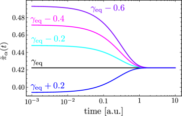
Figure 4: Plot of the changing IFP, denoted here by $\tilde{\pi}_{\alpha}(t)$, over time $t$ in logarithmic scale (for the plot we set the initial time $t^{*}=0$). The figure shows that $\tilde{\pi}_{\alpha}(t)\neq\pi_{\alpha}(\lambda_{t^{*}})$ unless we choose $\gamma=\gamma_{\text{eq}}$. In the long-time limit the IFP coincides with the equilibrium distribution (94). We set $\epsilon=1$ which implies $\gamma_{\text{eq}}\approx 0.73$.

This example proves that ergodicity does not imply that $\pi_{\alpha}(\lambda_{t})$ is the IFP of the reduced dynamics, as claimed in Ref. Speck and Seifert (2007) for arbitrary non-Markovian dynamics. Even 1-Markovianity together with ergodicity is not sufficient to ensure this statement.

VI.2 Markovianity without time-scale separation

We give a simple example of a physically relevant and lumpable Markov process although TSS does not apply. For this purpose consider the following rate matrix

$$W=\left(\begin{array}[]{ccc}-2\gamma_{\text{in}}&\gamma_{\text{out}}&\gamma_{\text{out}}\\ \gamma_{\text{in}}&-\gamma_{\text{out}}-\bar{\gamma}_{\text{flip}}&\gamma_{\text{flip}}\\ \gamma_{\text{in}}&\bar{\gamma}_{\text{flip}}&-\gamma_{\text{out}}-\gamma_{\text{flip}}\\ \end{array}\right)$$ (95)

describing the time evolution of a probability vector $\textbf{p}(t)=[p_{0}(t),p_{\uparrow}(t),p_{\downarrow}(t)]$. This ME describes a quantum dot in the ultrastrong Coulomb blockade regime coupled to a metallic lead taking the spin degree of freedom into account. Then, $p_{0/\uparrow/\downarrow}(t)$ are the probabilities to find the dot at time $t$ in a state with zero electrons, an electron with spin up or an electron with spin down, respectively. If the metallic lead has a finite magnetization, the rates for hopping in ($\gamma_{\text{in}}$) and out ($\gamma_{\text{out}}$) of the quantum depend on the spin, which can be derived from first principles Braun et al. (2004) and has interesting thermodynamic applications Strasberg et al. (2014). But if the lead has zero magnetization as considered here, the dynamics of the spin degree of freedom do not matter. Hence, if we consider the partition $\chi_{0}=\{0\}$ and $\chi_{1}=\{\uparrow,\downarrow\}$, it is not hard to deduce that

$$\frac{\partial}{\partial t}\binom{p_{0}(t)}{p_{1}(t)}=\left(\begin{array}[]{cc}-2\gamma_{\text{in}}&\gamma_{\text{out}}\\ 2\gamma_{\text{in}}&-\gamma_{\text{out}}\\ \end{array}\right)\binom{p_{0}(t)}{p_{1}(t)}$$ (96)

where $p_{1}(t)=p_{\uparrow}(t)+p_{\downarrow}(t)$. Thus, the coarse-grained dynamics is Markovian for all times $t$ and all micro initial conditions $[p_{0}(0),p_{\uparrow}(0),p_{\downarrow}(0)]$ although TSS does not apply. Notice that the IFP of Eq. (96) coincides with the marginalized IFP of Eq. (95) and hence, we have $\dot{\Sigma}(t)\geq 0$. Moreover, as long as the structure of the rate matrix (95) is preserved, we could have even allowed for arbitrary time-dependencies in the rates.

VI.3 Classical Brownian motion

We here present an example which exhibits negative EP rates and link their appearance to the spectral features of the environment. This is done by considering the important class of driven, classical Brownian motion models (also called Caldeira-Leggett or independent oscillator models). The global Hamiltonian with mass-weighted coordinates reads

$$H(\lambda_{t}) =\frac{1}{2}[p^{2}+\omega^{2}(\lambda_{t})x^{2}],$$ (97)

$$V+H_{B} =\frac{1}{2}\sum_{k}\left[p_{k}^{2}+\nu_{k}^{2}\left(x_{k}-\frac{c_{k}}{\nu_{k}^{2}}x\right)^{2}\right],$$ (98)

and its study has attracted considerable interest in strong coupling thermodynamics Martinez and Paz (2013); Pucci et al. (2013); Strasberg et al. (2016); Freitas and Paz (2017); Strasberg and Esposito (2017); Aurell (2017); Perarnau-Llobet et al. (2018); Hsiang et al. (2018). The Hamiltonian describes a central oscillator with position $x$ and momentum $p$ linearly coupled to a set of bath oscillators with positions $x_{k}$ and momenta $p_{k}$. The frequency of the central oscillator can be driven and we parametrize it as $\omega(\lambda_{t})=\omega_{0}+g\sin(\omega_{L}t)$. Furthermore, $c_{k}$ and $\nu_{k}$ are the system-bath coupling constants and the frequencies of the bath oscillators. It turns out that all the information about the bath (except of its temperature) can be encoded into a single function known as the spectral density of the bath. It is defined in general as $J(\omega)\equiv\frac{\pi}{2}\sum_{k}\frac{c_{k}^{2}}{\nu_{k}}\delta(\omega-\nu_{k})$ and we parametrize it as

$$J(\omega)=\frac{\lambda_{0}^{2}\gamma\omega}{(\omega^{2}-\omega_{1}^{2})^{2}+\gamma^{2}\omega^{2}}.$$ (99)

Here, $\lambda_{0}$ controls the overall coupling strength between the system and the bath and $\gamma$ changes the shape of the SD from a pronounced peak around $\omega_{1}$ for small $\gamma$ to a rather unstructured and flat SD for large $\gamma$. Thus, intuitively one expects that a smaller $\gamma$ corresponds to stronger non-Markovianity although this intuition can be misleading too Strasberg and Esposito (2018).

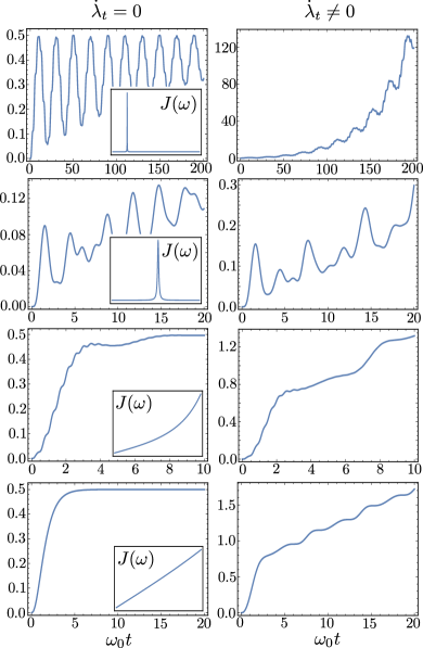
Figure 5: Plot of the dimensionless entropy production $\Sigma(t)$ ($k_{B}\equiv 1$) over the dimensionless time $\omega_{0}t$ for different parameters. For the driving we chose $g=0$ and $g=0.3\omega_{0}$ for the left or right column, respectively, and $\omega_{L}=\omega_{0}$. We changed the shape of the spectral density $J(\omega)$ in each row, which is depicted for $\omega\in[0,6\omega_{0}]$ as a small inset (note that the vertical scaling is different in each inset). Specifically, the parameters $(\lambda_{0},\gamma,\omega_{1})$ are $(0.316\omega_{0},0.01,1)\omega_{0}$ (top), $(3.16\omega_{0},0.1,3.16)\omega_{0}$ (second row), $(100\omega_{0},1,10)\omega_{0}$ (third row), $(500\omega_{0},10,31.6)\omega_{0}$ (bottom). The system was prepared according to Eq. (12) with initial mean values ${\left\langle{x}\right\rangle}(0)=(\sqrt{\beta}\omega_{0})^{-1}$, ${\left\langle{p_{x}}\right\rangle}(0)=0$ and covariances $C_{xx}(0)=(\beta\omega_{0}^{2})^{-1},C_{p_{x}p_{x}}(0)=\beta^{-1}$ and $C_{xp_{x}}(0)=0$. Note that this specific choice corresponds to equilibrated covariances, but the mean values are out of equilibrium. The general features of the plot, however, do not change too much for different non-equilibrium initial states. Finally, we set $\omega_{0}=1$ and $\beta=1$. See also Ref. Strasberg and Esposito (2017) for details of the computation.

The dynamics of the model is exactly described by the generalized Langevin equation (see, e.g., Weiss (2008))

$$\ddot{x}(t)+\omega_{0}^{2}(t)x(t)+\int_{0}^{t}ds\Gamma(t-s)\dot{x}(s)=\xi(t)$$ (100)

with the friction kernel

$$\Gamma(t)\equiv\int_{0}^{\infty}d\omega\frac{2}{\pi\omega}J(\omega)\cos(\omega t)$$ (101)

and the noise $\xi(t)$, which – when averaged over the initial state of the bath – obeys the statistics

$${\left\langle{\xi(t)}\right\rangle}_{B}=0,~{}~{}~{}{\left\langle{\xi(t)\xi(s)}\right\rangle}_{B}=\frac{1}{\beta}\Gamma(t-s).$$ (102)

To compute the thermodynamic quantities introduced in Sec. IV we need the state of the system $\rho_{S}(t)$. It can be computed with the method explained in Sec. IV of Ref. Strasberg and Esposito (2017), which we will not repeat here. Instead, we focus on the explanation of the numerical observations only.

Fig. 5 gives illustrative examples of the time-evolution of the EP $\Sigma(t)\geq 0$ defined in Eq. (71) for various situations. In total, we plot it for four different parameters characterizing the spectral density, always for the same initial condition of the system, but for the case of an undriven (left column) or a driven (right column) process. The parameters are chosen from top to bottom such that the spectral density resembles more and more an Ohmic spectral density $J(\omega)\sim\omega$, which usually gives rise to Markovian behaviour. In fact, this standard intuition is nicely confirmed in Fig. 5 by observing that negative EP rates are much larger and much more common at the top. The plot at bottom indeed corresponds to the Markovian limit in which the bath is conditionally equilibrated throughout (this is similar to the limit of TSS treated in Sec. III.3, see also Ref. Strasberg and Esposito (2017) for additonal details). It is worthwhile to repeat that a negative EP rate in the left column of Fig. 5 indicates non-Markovian behaviour in a rigorous sense, whereas for the right column this is only true in a weaker sense, but it unambiguously shows that the bath cannot be adiabatically eliminated.

VI.4 Quantum dynamics under the initial product state assumption

We have shown in Sec. V that the definition (24) of the EP rate for classical systems does not properly generalize to the quantum case. Part of the problem could be that we started from an initially correlated state, which complicates the treatment of the dynamics of the quantum system significantly. Therefore, one often resorts to the initial product state assumption $\hat{\rho}_{\text{tot}}(0)=\hat{\rho}_{S}(t)\otimes\hat{\rho}_{B}$, where $\hat{\rho}_{S}(t)$ is arbitrary and $\hat{\rho}_{B}$ fixed (usually taken to be the Gibbs state of the bath) Rivas et al. (2014); Breuer et al. (2016); Breuer and Petruccione (2002); de Vega and Alonso (2017); Esposito et al. (2010). It is then interesting to ask which general statements connecting Markovianity, the notion of an IFP and EP rates can be made in this case. The following simple example shows which statements do not hold in this case.

A single fermionic mode (such as a quantum dot in the Coulomb blockade regime) tunnel-coupled to a bath of free fermions (describing, e.g., a metallic lead) can be modeled by the single resonant level Hamiltonian (assuming spin polarization)

$$\hat{H}_{\text{tot}}=\epsilon_{0}\hat{d}^{\dagger}\hat{d}+\sum_{k}\left(t_{k}\hat{d}\hat{c}_{k}^{\dagger}+t_{k}^{*}\hat{c}_{k}\hat{d}^{\dagger}+\epsilon_{k}\hat{c}_{k}^{\dagger}\hat{c}_{k}\right).$$ (103)

Here, $\hat{d}^{(\dagger)}$ and $\hat{c}_{k}^{(\dagger)}$ are fermionic annihilation (creation) operators, $\epsilon_{0}$ is the real-valued energy of the quantum dot, $t_{k}$ is a complex tunnel amplitude and $\epsilon_{k}$ is the real-valued energy of a bath fermion.

To describe the dynamics of the open system we use the Redfield ME Breuer and Petruccione (2002); de Vega and Alonso (2017)

$$\frac{\partial}{\partial t}\hat{\rho}_{S}(t) =-i[\hat{H},\hat{\rho}_{S}(t)]$$ (104)

$$-\int_{0}^{t}ds\mbox{tr}_{B}\left\{[\hat{V},[\hat{V}(s-t),\hat{\rho}_{S}(t)\otimes\hat{\pi}_{B}]]\right\}.$$

Here, the system and interaction Hamiltonian are $\hat{H}=\epsilon_{0}\hat{d}^{\dagger}\hat{d}$ and $\hat{V}=\sum_{k}(t_{k}\hat{d}\hat{c}_{k}^{\dagger}+t_{k}^{*}\hat{c}_{k}\hat{d}^{\dagger})$. Furthermore, $\hat{V}(t)=e^{i(\hat{H}+\hat{H}_{B})t/\hbar}\hat{V}e^{-i(\hat{H}+\hat{H}_{B})t/\hbar}$ denotes the interaction picture with $\hat{H}_{B}=\sum_{k}\epsilon_{k}\hat{c}_{k}^{\dagger}\hat{c}_{k}$. We assumed the initial system-bath state to be $\hat{\rho}_{S}(0)\otimes\hat{\pi}_{B}$ where $\hat{\rho}_{S}(0)$ is arbitrary and $\hat{\pi}_{B}$ the grand-canonical equilibrium state with respect to $\hat{H}_{B}$ and the particle number operator $\hat{N}_{B}=\sum_{k}\hat{c}_{k}^{\dagger}\hat{c}_{k}$. Without loss of generality we set the chemical potential to zero ($\mu=0$). The Redfield equation (104) directly results from a perturbative expansion of the exact time-convolutionless ME and it gives accurate results for sufficiently small tunneling amplitudes $t_{k}$ and a relatively high bath temperature.

Following standard procedures, we rewrite Eq. (104) as

$$\frac{\partial}{\partial t}\hat{\rho}_{S}(t)= -i\epsilon(t)[\hat{d}^{\dagger}\hat{d},\hat{\rho}_{S}(t)]$$ (105)

$$+\gamma_{\text{out}}(t)\left(\hat{d}\hat{\rho}_{S}(t)\hat{d}^{\dagger}-\frac{1}{2}\{\hat{d}^{\dagger}\hat{d},\hat{\rho}_{S}(t)\}\right)$$

$$+\gamma_{\text{in}}(t)\left(\hat{d}^{\dagger}\hat{\rho}_{S}(t)\hat{d}-\frac{1}{2}\{\hat{d}\hat{d}^{\dagger},\hat{\rho}_{S}(t)\}\right),$$

where $\{\cdot,\cdot\}$ denotes the anti-commutator and $\epsilon(t)\equiv\epsilon_{0}-\Delta_{\text{in}}(t)-\Delta_{\text{out}}(t)$ is a time-dependent renormalized system energy. In detail, we have introduced the quantities

$$\gamma_{\text{in}}(t) \equiv\int_{0}^{t}d\tau\int_{-\infty}^{\infty}d\omega\frac{J(\omega)}{\pi}f(\omega)\cos[(\omega-\epsilon_{0})\tau],$$ (106)

$$\Delta_{\text{in}}(t) \equiv\int_{0}^{t}d\tau\int_{-\infty}^{\infty}d\omega\frac{J(\omega)}{2\pi}f(\omega)\sin[(\omega-\epsilon_{0})\tau],$$ (107)

$$\gamma_{\text{out}}(t) \equiv\int_{0}^{t}d\tau\int_{-\infty}^{\infty}d\omega\frac{J(\omega)}{\pi}[1-f(\omega)]\cos[(\omega-\epsilon_{0})\tau],$$ (108)

$$\Delta_{\text{out}}(t) \equiv\int_{0}^{t}d\tau\int_{-\infty}^{\infty}d\omega\frac{J(\omega)}{2\pi}[1-f(\omega)]\sin[(\omega-\epsilon_{0})\tau],$$ (109)

where $f(\omega)\equiv(e^{\beta\omega}+1)^{-1}$ denotes the Fermi function for $\mu=0$ and $J(\omega)\equiv 2\pi\sum_{k}|t_{k}|^{2}\delta(\omega-\epsilon_{k})$ is the spectral density of the bath. If there are no initial coherences in the quantum dot present, we can conclude without any further approximation that the full dynamics of the quantum dot is captured by the rate ME

$$\frac{\partial}{\partial t}\binom{p_{1}(t)}{p_{0}(t)}=\left(\begin{array}[]{cc}-\gamma_{\text{out}}(t)&\gamma_{\text{in}}(t)\\ \gamma_{\text{out}}(t)&-\gamma_{\text{in}}(t)\\ \end{array}\right)\binom{p_{1}(t)}{p_{0}(t)},$$ (110)

where $p_{1}(t)$ [$p_{0}(t)$] describes the probability to find the dot in the filled [empty] state at time $t$.

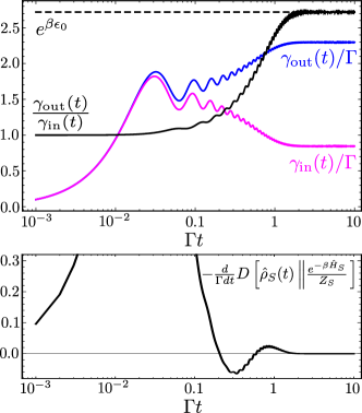
Figure 6: Top: Plot of the (dimensionless) rates $\gamma_{\text{in}}(t)/\Gamma$ and $\gamma_{\text{out}}(t)/\Gamma$ defined in Eqs. (106) and (108), their ratio $\gamma_{\text{out}}(t)/\gamma_{\text{in}}(t)$ and the expected local detailed balance ratio $e^{\beta\epsilon_{0}}$ over dimensionless time $\Gamma t$ in logarithmic scale. For the plot we parametrized the bath spectral density as $J(\omega)=\Gamma$ for $\omega/\Gamma\in[-100,+100]$ and zero outside. The dot energy and inverse temperature of the bath are set to $\epsilon_{0}=\beta=1$. Bottom: For the same parameters we plot an often used canditate for the EP rate over dimensionless time $\Gamma t$ in logarithmic scale for the initial state $p_{1}(0)=0.1,p_{0}(0)=0.9$.

We now investigate the IFP of the dynamics. In Fig. 6 (top) we plot the time evolution of the rates $\gamma_{\text{in}}(t)$ and $\gamma_{\text{out}}(t)$ as well as their ratio. We see that for long times they become stationary and their ratio fulfills local detailed balance (33), which implies that the steady state is a Gibbs state and hence, the system properly thermalizes. However, for short times, the ratio does not fulfill local detailed balance and hence, the IFP is not the Gibbs state. Furthermore, as the rates are positive all the time, the dynamics is clearly 1-Markovian. This proves that a 1-Markovian time-evolution, which yields the correct long-time equilibrium state, can nevertheless have a time-dependent IFP, even if the underlying Hamiltonian is time-independent. This clearly shows that 1-Markovian evolution does not imply a time-invariant IFP as claimed in the literature [see, e.g., below Eq. (47) in Ref. de Vega and Alonso (2017) or Eq. (9) in Ref. Thomas et al. (2018)].

In addition, Fig. 6 (bottom) also shows the time evolution of

$$\dot{\sigma}(t)\equiv-\frac{\partial}{\partial t}D[\hat{\rho}_{S}(t)\|e^{-\beta\hat{H}_{S}}/Z_{S}]$$ (111)

In the weak coupling limit it is tempting to identifiy $\dot{\sigma}(t)$ as the EP rate because the global equilibrium state can be approximated by $\hat{\pi}_{SB}\approx e^{-\beta\hat{H}_{S}}/Z_{S}\otimes e^{-\beta\hat{H}_{B}}/Z_{B}$. However, one should be cautious here as this is not an exact result and the initial product state assumption does not fit into the description used in Secs. IV and V. The transient dynamics is indeed dominated by the build-up of system-bath correlations and an exact treatment needs to take them into account Esposito et al. (2010). Therefore, outside the specific limit of the Born-Markov secular master equation, where $\dot{\sigma}(t)$ can be related to the actual EP rate Spohn and Lebowitz (1979); Spohn (1978), the quantity $\dot{\sigma}(t)$ lacks a clear connection to a consistent thermodynamic framework. In addition, Fig. 6 clearly demonstrates that $\dot{\sigma}(t)<0$ is possible although the dynamics is 1-Markovian. For these reasons the claimed connections between a negative “entropy production” rate $\dot{\sigma}(t)$ and non-Markovianity in Refs. Argentieri et al. (2014); Bhattacharya et al. (2017); Marcantoni et al. (2017); Popovic et al. (2018) require a careful reassessment.

VII Summary and outlook

VII.1 Summary

A large part of this paper was devoted to study the instantaneous thermodynamics at the rate level for an arbitrary classical system coupled to a single heat bath. Quite remarkably, the definition of the EP rate (2) for a weakly coupled Markovian system can be carried over to the strong-coupling and non-Markovian situation if we replace the Gibbs state with the correct equilibrium state $\pi_{\alpha}(\lambda_{t})$, described, e.g., by the Hamiltonian of mean force Kirkwood (1935). The EP rate then reads

$$\dot{\Sigma}(t)\equiv-\left.\frac{\partial}{\partial t}\right|_{\lambda_{t}}D[p_{\alpha}(t)\|\pi_{\alpha}(\lambda_{t})].$$ (112)

Starting from this definition together with an unambiguous definition for work [Eqs. (43) and (66)], we recovered the previously proposed definitions in Refs. Seifert (2016); Miller and Anders (2017); Strasberg and Esposito (2017). Most importantly, we were able to connect the abstract concept of (non-) Markovianity to the physical observable consequence of having a negative EP rate $\dot{\Sigma}(t)<0$. We can summarize our finding as follows:

Theorem.

If the dynamics are undriven ($\dot{\lambda}_{t}=0$), any appearance of $\dot{\Sigma}(t)<0$ unambiguously reveals that the dynamics is non-Markovian. If the dynamics is driven ($\dot{\lambda}_{t}\neq 0$), any appearance of $\dot{\Sigma}(t)<0$ unambiguously reveals that the dynamics is non-Markovian or that $\pi_{\alpha}(\lambda_{t})$ cannot be an IFP of the dynamics. This implies that TSS does not apply.

Especially for the undriven case, it was important to study the question when is the equilibrium state $\pi_{\alpha}(\lambda_{t})$ also an IFP of the dynamics. To the best of our knowledge, this was not yet studied thoroughly. In particular, a 1-Markovian evolution of the system does not imply that $\pi_{\alpha}(\lambda_{t})$ is an instantaneous fixed point of the dynamics. This is the reason why a 1-Markovian evolution alone is not sufficent to imply that the entropy production rate is always positive. Fig. 7 shows the mathematical implications and equivalences worked out in this paper.

Figure 7: Overview of the results from Secs. II, III and IV (the notation is chosen as in Secs. II and III, but the findings are identical to Sec. IV). The arrows indicate implications in a mathematical sense. Some implications depend on certain conditions, which are marked by a line attached with a circle to the respective arrow.

We then left the classical regime and provided a thermodynamic framework for a strongly coupled, driven quantum system immersed in an arbitrary heat bath in Sec. V. Inspired by the classical treatment and backed up by equilibrium considerations using the quantum Hamiltonian of mean force Hänggi et al. (2008); Gelin and Thoss (2009); Hsiang and Hu (2018), we defined internal energy $U$, system entropy $S$ and free energy $F$ [Eqs. (80) to (82)] for a quantum system arbitrarily far from equilibrium. Remarkably, the basic definitions are formally identical to the classical case albeit they were critically debated in Refs. Hänggi et al. (2008); Gelin and Thoss (2009). Nevertheless, they ensure that the first and second law as known from phenomenological non-equilibrium thermodynamics, $\Delta U=Q+W$ and $\Sigma=\beta(W-\Delta F)=\Delta S-\beta Q\geq 0$, also hold in the quantum regime. Thus, at the integrated level the quantum nature of the interaction becomes manifest only by realizing that we can treat a smaller class of admissible initially correlated states. At the rate level, however, we showed that the quantum generalization of Eq. (112) does not coincide with the entropy production rate $\dot{\Sigma}(t)=\beta[\dot{W}(t)-d_{t}F(t)]$. Thus, at present it seems that there is no rigorous connection between negative entropy production rates and non-Markovianity.

To support the latter statement we also investigated in Sec. VI.4 what happens for initially decorrelated states if we use the conventional definition of entropy production rate [i.e., the quantum counterpart of Eq. (2)] valid in the limit of the Born-Markov-secular approximation Spohn (1978); Spohn and Lebowitz (1979); Lindblad (1983); Breuer and Petruccione (2002); Kosloff (2013). Unfortunately, outside this limit this definition does not provide an adequate candidate for an entropy production rate and even for a weakly coupled and 1-Markovian system it can be transiently negative. From the perspective of open quantum system theory, this behaviour is caused by the initial build-up of system-environment correlations, which – even in the weak coupling limit – cannot be neglected and need to be taken into account in any formally exact thermodynamic framework Esposito et al. (2010).

Table 2 summarizes what is known (and what not) about the thermodynamic description of a driven system coupled to a single heat bath for the classical (abbreviated CM) and the quantum (QM) case, respectively.

	CM	QM
Consistent with equilibrium thermodynamics(a)	✓	✓
Nonequilibrium first law	✓	✓
Nonequilibrium second law	✓	✓
Recovery of weak-coupling limit	✓	✓
Jarzynski-Crooks work fluctuation theorem(b)	✓	✓
Entropy production fluctuation theorem(c)	✓	↯
Arbitrary initial system states	✓	↯
Consistent with TSS	✓	↯
Connection to non-Markovianity	✓	↯

Table 2: Current state-of-the-art of strong coupling thermodynamics for a single heat bath. The ↯-symbol indicates only that it is currently not known how to establish the corresponding quantum version. Remarks: (a) We here mean that the standard textbook relations between the partition function and internal energy, entropy and free energy are recovered at equilibrium. (b) A work fluctuation theorem of the “Jarzynski-Crooks” type starts with a process in equilibrium and contains the equilibrium free energies in the expression. (c) An entropy production (or “integral”) fluctuation theorem allows to start in a non-equilibrium state and contains the nonequilibrium free energies.

VII.2 Outlook

After having established a general theoretical description involving a lot of mathematical details, we here take the freedom to be less precise in order to discuss various consequences of our findings and to point out interesting open research avenues.

First of all, the field of strong coupling and non-Markovian thermodynamics is far from being settled and many different approaches have been put forward. Therefore, one might wonder whether the definitions we have used here are the “correct” ones or whether one should not start with a completely different set of definitions. We believe that the definitions we have used possess a certain structural appeal: we could establish a first and second law as known from phenomenological non-equilibrium thermodynamics and in the limit of TSS or at equilibrium, our definitions coincide with established results from the literature. Furthermore, the fact that in the classical case we could give to the appearance of a negative EP rate a clear dynamical meaning adds further appeal to the definitions used here.

On the other hand, this last point is lost for quantum systems leaving still a larger room of ambiguity there. In this respect, it is also worth to point out that for strongly coupled, non-Markovian systems it was also possible to find definitions which guarantee an always positive EP rate even in presence of multiple heat baths. One possibility is to redefine the system-bath partition Strasberg and Esposito (2017); Strasberg et al. (2016); Newman et al. (2017); Schaller et al. (2018); Strasberg et al. (2018); Restrepo et al. (2018), which reverses the strategy of Sec. III: instead of looking at the mesostates only when starting from a consistent description in terms of the microstates, one starts with a mesoscopic description and ends up with a consistent description in a larger space, i.e., one effectively finds the microstates from Sec. III. Alternatively and without enlarging the state space, Green’s functions techniques can be used for simple models to define an always positive EP rate Esposito et al. (2015); Bruch et al. (2016); Ludovico et al. (2016); Haughian et al. (2018) or the Polaron transformation can be useful when dealing with particular strong coupling situations Schaller et al. (2013); Krause et al. (2015); Gelbwaser-Klimovsky and Aspuru-Guzik (2015); Wang et al. (2015); Friedman et al. (2018).

Applying our present framework in context of multiple heat baths poses a formidable challenge as it remains unclear what the correct reference state $\pi_{\alpha}(\lambda_{t})$ should be. While it is known how to extend the second law (2) to multiple heat baths if the Born-Markov secular approximation is applied Spohn and Lebowitz (1979), this approximation can be unjustified even at weak coupling Mitchison and Plenio (2018). Furthermore, the correct choice of initial state plays a crucial role as it can lead to different thermodynamic definitions; compare, e.g., with the initial product state assumption used in Ref. Esposito et al. (2010). At the end, we believe that the most meaningful thermodynamic description will indeed depend on the question which degrees of freedom we can measure and control in an experiment. However, at least at steady state many of the different approaches coincide because the system-bath boundary then usually contributes only a time-independent additive constant to the description.

Within the framework we have used here, we can get also more insights by viewing our findings in light of the recent endeavour to find a meaningful quantifier of non-Markovianity for quantum systems Rivas et al. (2014); Breuer et al. (2016). At least for classical, undriven systems it seems reasonable to measure the degree of non-Markovianity via the quantity

$${\cal{N}}\equiv\max_{p_{x}(0)\in{\cal{A}}_{\pi}}\int_{\dot{\Sigma}(t)<0}\left|\dot{\Sigma}(t)\right|dt\geq 0.$$ (113)

The larger ${\cal{N}}$, the stronger the system behaves non-Markovian. This quantifier shares structural similarity with the BLP quantifier Breuer et al. (2009) and a non-zero value could be likewise interpreted as information backflow from the bath to the system. Thus, our findings show that due to memory effects $\dot{\Sigma}(t)$ looses its property of a Lyapunov function. Of course, ${\cal{N}}$ presents just one out of a multitude of possible non-Markovianity quantifiers Rivas et al. (2014); Breuer et al. (2016), but it has the outstanding advantage that it is clearly linked to an important and meaningful physical quantitiy. Its comparison with other measures therefore deserves further attention.

To close this paper, we ask for which problems non-Markovian effects could be beneficial in a thermodynamic sense. This question constitutes in principle a vast field on its own, which we only want to briefly touch. A central benefit of non-Markovian dynamics is that new state transformations become possible, which are not realizable with a Markovian finite time dynamics. We here want to give a simple example of physical and thermodynamic relevance to illustrate the main point. This example is the erasure of a single bit of information.

Erasing a single bit of information is related to Landauer’s famous principle Landauer (1961) and it is nowadays possible to measure the minuscule thermodynamic changes associated to this transformation Orlov et al. (2012); Bérut et al. (2012); Jun et al. (2014); Bérut et al. (2015); Gavrilov and Bechhoefer (2016); Hong et al. (2016); Yan et al. (2018). Theoretically, the process of erasure is usually modeled with a Markovian two-state system and optimal protocols have been investigated in Refs. Diana et al. (2013); Zulkowski and DeWeese (2014). Let us now illustrate which benefits non-Markovian dynamics can add. We denote the two states of the bit by “0” and “1” and model the dynamics by the ME

$$\frac{\partial}{\partial t}\binom{p_{1}(t)}{p_{0}(t)}=\left(\begin{array}[]{cc}-\gamma_{01}(t)&\gamma_{10}(t)\\ \gamma_{01}(t)&-\gamma_{10}(t)\\ \end{array}\right)\binom{p_{1}(t)}{p_{0}(t)}.$$ (114)

Since we have not made any assumptions about the time-dependent rates $\gamma_{01}(t)$ and $\gamma_{10}(t)$, this model is general and could be obtained directly from Eq. (19). Note that the origin of the time-dependence of the rates does not need to come from any driving, cf. Eqs. (19) or (110). From $p_{0}(t)+p_{1}(t)=1$ we obtain a linear, inhomogeneous differential equation with time-dependent coefficients for the probability to be in state zero. It reads $\dot{p}_{0}(t)=\gamma_{01}(t)-[\gamma_{10}(t)+\gamma_{01}(t)]p_{0}(t)$ with the formal solution

$$p_{0}(t)= ~{}\exp\left[-\int_{0}^{t}ds[\gamma_{10}(s)+\gamma_{01}(s)]\right]p_{0}(0)$$ (115)

$$+\int_{0}^{t}ds\exp\left[-\int_{s}^{t}du[\gamma_{10}(u)+\gamma_{01}(u)]\right]\gamma_{01}(s).$$

For definiteness we choose to erase the bit such that the probability $p_{0}(t)$ to find the bit in state zero is as large as possible at time $t$.

Now, as a proof of principle, let us assume that $\gamma_{01}(t)\geq 0$ for all times $t$, but $\gamma_{10}(t)$ can be negative for certain times, which clearly indicates non-Markovian behaviour. Furthermore, we denote the fact that $p_{0}(t)$ depends on the whole history of $\gamma_{10}(t)$ by $p_{0}(t)=p_{0}[t;\{\gamma_{10}(t)\}]$. Next, we recall the well-known inequality $\int_{0}^{t}dsf(s)\leq\int_{0}^{t}ds|f(s)|$ for any time-dependent function $f(t)$, which implies

$$\exp\left[-\int_{0}^{t}dsf(s)\right]\geq\exp\left[-\int_{0}^{t}ds|f(s)|\right].$$ (116)

Because the two terms in Eq. (115) are separately positive, this inequality implies

$$p_{0}[t;\{\gamma_{10}(t)\}]\geq p_{0}[t;\{|\gamma_{10}(t)|\}]$$ (117)

for any initial state and independent of the precise form of the rates. In fact, if for certain times $\gamma_{10}(t)<0$ we have a strict inequality: $p_{0}[t;\{\gamma_{10}(t)\}]>p_{0}[t;\{|\gamma_{10}(t)|\}]$. This shows that non-Markovian effects can help erase a bit faster in finite time.

To conclude, we believe that our work paves the way for a rigorous understanding of finite-time thermodynamics away from the conventional Markovian assumption. Because our understanding of finite-time processes has drastically improved during the last years Deffner and Campbell (2017), exploring their thermodynamic implications opens up a new and exciting research field.

Acknowledgements

This research is funded by the European Research Council project NanoThermo (ERC-2015-CoG Agreement No. 681456).

Appendix A Weak lumpability

The notion of lumpability required the coarse-grained Markov chain to be Markovian for any initial microstate. One might wonder what can be said about the dynamics if there is at least one initial microstate which leads to a Markov chain at the mesolevel. For this purpose Kemeny and Snell introduce the concept of weak lumpability (Sec. 6.4. in Ref. Kemeny and Snell (1976)):

Definition A.1 (Weak lumpability).

A Markov chain is weakly lumpable with respect to a partition $\boldsymbol{\chi}$ if there exists at least one initial distribution $p_{x}(0)$ such that the lumped process is a Markov chain. The TM can then depend on $p_{x}(0)$.

The fact that the TMs for a weakly lumpable process can depend on the initial microstate $p_{x}(0)$ is also apparent in Eq. (8). Furthermore, it is again clear that a weakly lumpable process with respect to $p_{x}(0)$ for a given TM $T_{\tau}$ and partition $\boldsymbol{\chi}$, is also a weakly lumpable process with respect to $p_{x}(0)$ for all larger times, i.e., for all $T_{n\tau}=(T_{\tau})^{n}$ with $n>1$ and the same partition $\boldsymbol{\chi}$.

The concept of weak lumpability is especially useful when the underlying Markov chain is regular:

Definition A.2 (Regular Markov chain).

A Markov chain is called regular if there exists an $n\in\mathbb{N}$ such that all elements of the matrix $T^{n}_{\tau}$ are strictly positive.

A regular Markov chain ensures that the system reaches its steady state $\boldsymbol{\pi}=\lim_{n\rightarrow\infty}T^{n}_{\tau}\textbf{p}(0)$ for any initial distribution $\textbf{p}(0)$ and hence, it has a unique steady state. Kemeny and Snell then prove the following Kemeny and Snell (1976):

Theorem A.1.

Assume that a regular Markov chain with steady state $\pi_{x}$ is weakly lumpable with respect to the partition $\boldsymbol{\chi}$ for some initial distribution $p_{x}(0)$. Then, the Markov chain is also weakly lumpable for the initial distribution $\pi_{x}$ with the same transition probabilities, which are determined by

$$G_{\tau}(\alpha|\beta)=\sum_{x_{\alpha},y_{\beta}}T_{\tau}(x_{\alpha}|y_{\beta})\pi_{y|\beta}.$$ (118)

Thus, Theorem A.1 says that for a regular and weakly lumpable Markov chain we can always use the conditional steady state $\pi_{x|\alpha}$ to construct the TM at the mesolevel and do not need to use $p_{x|\alpha}(0)$ as in Eq. (8). This is advantageous to say something about the IFP of undriven processes:

Theorem A.2.

Consider an undriven stochastic process described by the ME (19), i.e., we assume $G_{t,0}^{-1}$ to exist for all admissible initial states ${\cal{A}}(0)$ and all times $t$. If the stochastic process is weakly lumpable for an underlying regular Markov chain with respect to an admissible initial state $p_{x}(0)\in{\cal{A}}(0)$, then $\pi_{\alpha}$ is a IFP of the stochastic process at the mesolevel.

Proof.

Using the insights from Theorem A.1, it becomes clear that $\sum_{\beta}G_{t,0}(\alpha|\beta)\pi_{\beta}=\pi_{\alpha}$ for all times $t$. Together with the invertibility condition we also get Eq. (30) from the main text. These two relations were all we needed to ensure that Eq. (LABEL:eq_help_thm_steady_state_weak) holds. ∎

To conclude, as most physically relevant Markov chains are regular, the concept of weak lumpability helps us to deal with initial conditions, where the microstates have not reached a conditional steady state. Together with Theorem II.2 this would then imply an always positive EP rate because a weakly lumpable process with respect to an admissible initial state $p_{x}(0)\in{\cal{A}}(0)$ is also 1-Markovian with respect to that state.

However, a weakly lumpable process still requires the whole hierarchy to fulfill the Markov condition (7) and also on physical grounds we expect that it is a good approximation to assume that the conditional initial microstates are at steady state. If this is the case, then the notion of weak lumpability does not seem to add any further insights into the theory of Secs. III and IV.

Appendix B Instantaneous fixed points and time-local master equation

Formally exact time-local ME can be derived in different ways. One particular construction was given in Eq. (20), but another possibility is given by the time-convolutionless ME Breuer and Petruccione (2002); de Vega and Alonso (2017); Fulinski and Kramarczyk (1968); Shibata et al. (1977) and see Ref. Andersson et al. (2007) for yet another way of construction. We will here show that, as long as the inverse of the TM $G_{t,0}$ defined in Eq. (18) exists, the generators all coincide. Hence, the IFP computed with any of those time-local MEs is the same and therefore the IFP is a well-defined concept.

To see this, let us denote by $V^{(1)}(t)$ and $V^{(2)}(t)$ the generators of an exact time-local ME derived in two different ways (we suppress the depencence on $\lambda_{t}$ here for simplicity). Because both are assumed to be formally exact for any admissible initial condition, we have

$$\sum_{\beta}[V_{\alpha,\beta}^{(1)}(t)-V_{\alpha,\beta}^{(2)}(t)]p_{\beta}(t)=0$$ (119)

for any mesostate $p_{\beta}(t)$, which is reachable from the class of admissible initial states ${\cal{A}}(0)$. This equation also holds for any linear combination of such states, i.e.,

$$\sum_{i}\mu_{i}\sum_{\beta}[V_{\alpha,\beta}^{(1)}(t)-V_{\alpha,\beta}^{(2)}(t)]p^{(i)}_{\beta}(t)=0$$ (120)

with $\mu_{i}\in\mathbb{R}$. We now use that $G_{t,0}$ is invertible for any finite $t$, which implies in particular that the dimension of the image of $G_{t,0}$ cannot decrease. But since the class of admissible initial states spans the entire vector space including all probability distributions $p_{\beta}(t)$, we can always choose

$$\sum_{i}\mu_{i}p^{(i)}_{\beta}(t)=\delta_{\beta,\beta^{\prime}}$$ (121)

for any $\beta^{\prime}$. This implies that $V_{\alpha,\beta^{\prime}}^{(1)}(t)-V_{\alpha,\beta^{\prime}}^{(2)}(t)=0$ for any $\alpha$ and $\beta^{\prime}$. Hence, $V^{(1)}(t)=V^{(2)}(t)$.

Appendix C Fixed points of coarse-grained Hamiltonian dynamics

In this appendix we rederive those results from Sec. II, which will be of relevance for Sec. IV. Let us start with an arbitrary Hamiltonian $H(\lambda_{t})$ and an arbitrary fixed partition $\boldsymbol{\chi}$. The “master equation” corresponding to this Hamiltonian is the Liouville equation

$$\frac{\partial}{\partial t}\rho(x;t)=\{H(x;\lambda_{t}),\rho(x;t)\},$$ (122)

where $\{\cdot,\cdot\}$ denotes the Poisson bracket and $\rho(x;t)$ is the probability distribution defined on the phase space consisting of the collection of all positions q and momenta p. For simplicity and analogy with the main text we denote a point in phase space by $x=(\textbf{q},\textbf{p})$. For any partition $\boldsymbol{\chi}$, the mesostates are defined as

$$\rho(\alpha;t)=\int_{\chi_{\alpha}}dx\rho(x;t),$$ (123)

where $\alpha$ can be continuous (e.g., if we trace out a bath) or discrete (e.g., if we lump the motion of a particle in a double well potential into two states “left” and “right”). Furthermore, it turns out to be convenient to denote the dynamical map generated by Eq. (122) over a finite time interval by $\Phi_{t,0}$, i.e.,

$$\rho(x;t)=\int dx^{\prime}\Phi_{t,0}(x|x^{\prime})\rho(x^{\prime};0),$$ (124)

similar to the time-evolution operator in quantum mechanics.

Clearly, as in Sec. II for a given conditional initial microstate $\rho(x|\alpha;0)$, $\Phi_{t,0}$ induces a map at the mesolevel,

$$\rho(\alpha;t) =\int d\beta{\cal{G}}_{t,0}(\alpha|\beta)\rho(\beta;0),$$ (125)

$${\cal{G}}_{t,0}(\alpha|\beta) \equiv\int_{\chi_{\alpha}}dx\int_{\chi_{\beta}}dx^{\prime}\Phi_{t,0}(x|x^{\prime})\rho(x^{\prime}|\beta;0).$$ (126)

Using the procedure outlined in Sec. II.2 or the time-convolutionless ME Fulinski and Kramarczyk (1968); Shibata et al. (1977); Breuer and Petruccione (2002); de Vega and Alonso (2017), we write the time evolution of the mesostate again in terms of a formally exact ME [cf. Eq. (19)]

$$\frac{d}{dt}\rho(\alpha;t)={\cal{V}}(\lambda_{t},t)\rho(\alpha;t).$$ (127)

We note that the Hamiltonian dynamics generated by $\Phi_{t,s}$ ($t\geq s$) are Markovian. It is therefore possible to straightforwardly extend the definition of lumpability to Hamiltonian dynamics for any propagator $\Phi_{t,s}$. We will here choose a version for the infinitesimal propagator $\Phi_{t+\delta t,t}$ which is most useful in the following.

Definition C.1 (Lumpability – continuous version).

The dynamics generated by Eq. (122) is lumpable with respect to the partition $\boldsymbol{\chi}$ if for every initial distribution $\rho(x;0)$ the lumped process is Markovian and the generator ${\cal{V}}(\lambda_{t},t)$ in Eq. (127) does not depend on $\rho(x;0)$.

We now formulate the analogue of Theorem II.3:

Theorem C.1.

If the stochastic process is lumpable as in Definition C.1 for some time-interval $I$, then the IFP of the system is given by the marginal global Gibbs state with respect to $H(x;\lambda_{t})$ for all $t\in I$, i.e., ${\cal{V}}(\lambda_{t},t)\pi(\alpha;\lambda_{t})=0$ with

$$\pi(\alpha;\lambda_{t})=\int_{\chi_{\alpha}}dx\frac{e^{-\beta H(x;\lambda_{t})}}{Z(\lambda_{t})}.$$ (128)

Proof.

By assumption, the dynamics of the system is generated by

$$\begin{split}\frac{d}{dt}\pi(\alpha;\lambda_{t})&={\cal{V}}(\lambda_{t},t)\pi(\alpha;\lambda_{t})\\ &=\int_{\chi_{\alpha}}dx\{H(x;\lambda_{t}),\pi(\alpha;\lambda_{t})\rho(x|\alpha;t)\},\end{split}$$ (129)

where $\rho(x|\alpha;t)$ is so far an unknown conditional microstate and where we used that the reduced dynamics from Eq. (127) is formally exact and thus, they coincide with the coarse-grained global dynamics.

Next, by assumption of lumpability, we know that ${\cal{V}}(\lambda_{t},t)$ is the same for any initial state. Let us choose the particular initial state

$$\rho(x;0)=\Phi_{t,0}^{-1}\pi(x;\lambda_{t}),$$ (130)

which is obtained by evolving the Gibbs state $\pi(x;\lambda_{t})$ at time $t$ backward in time. Since the global dynamics is Hamiltonian, we remark that the inverse of $\Phi_{t,0}$ exists and maps well-defined probability distribution onto well-defined probability distributions. But for this choice we clearly have

$$\frac{d}{dt}\pi(\alpha;\lambda_{t})=\int_{\chi_{\alpha}}dx\{H(x;\lambda_{t}),\pi(x;\lambda_{t})\}=0.$$ (131)

This implies the theorem. ∎

In principle, of course, we expect the concept of lumpability to be of limited use for Hamiltonian dynamics. However, we can also establish the first part of Theorem II.4 for Hamiltonian dynamics:

Theorem C.2.

Consider an undriven Hamiltonian. If the set of admissible initial states obeys ${\cal{A}}(0)\subset{\cal{A}}_{\pi}$, then $\pi(\alpha)$ is a IFP of the stochastic process at the mesolevel.

The proof is identical to the first part of the proof of Theorem II.4. Furthermore, as in Theorem II.5 this also holds for the time-dependent case whenever ${\cal{A}}(t)\subset{\cal{A}}_{\pi}(\lambda_{t})$ or $\pi(x;\lambda_{t})\in{\cal{A}}(t)$.

Finally, Theorem II.2 then follows analogously by replacing the discrete relative entropy by its differential version and by noting that a proper generalization of Lemma II.1 holds also for infinite dimensions Spohn (1978).

References

- Hill (1977) T. L. Hill, Free Energy Transduction in Biology (Academic, New York, 1977).
- Spohn (1980) H. Spohn, “Kinetic equations from Hamiltonian dynamics: Markovian limits,” Rev. Mod. Phys. 52, 569–615 (1980).
- van Kampen (2007) N. G. van Kampen, Stochastic Processes in Physics and Chemistry (North-Holland Publishing Company, Amsterdam, 3rd ed., 2007).
- Breuer and Petruccione (2002) H.-P. Breuer and F. Petruccione, The Theory of Open Quantum Systems (Oxford University Press, Oxford, 2002).
- Kemeny and Snell (1976) J. G. Kemeny and J. L. Snell, Finite Markov Chains (Springer-Verlag, New York, 1976).
- Breuer et al. (2009) H. P. Breuer, E.-M. Laine, and J. Piilo, “Measure for the degree of non-Markovian behavior of quantum processes in open systems,” Phys. Rev. Lett. 103, 210401 (2009).
- Rivas et al. (2014) A. Rivas, S. F. Huelga, and M. B. Plenio, “Quantum non-Markovianity: Characterization, quantification and detection,” Rep. Prog. Phys. 77, 094001 (2014).
- Breuer et al. (2016) H.-P. Breuer, E.-M. Laine, J. Piilo, and B. Vacchini, “Colloquium: Non-Markovian dynamics in open quantum systems,” Rev. Mod. Phys. 88, 021002 (2016).
- Schnakenberg (1976) J. Schnakenberg, “Network theory of microscopic and macroscopic behavior of master equation systems,” Rev. Mod. Phys. 48, 571–585 (1976).
- Jiang et al. (2004) D.-Q. Jiang, M. Qian, and M.-P. Qian, Mathematical Theory of Nonequilibrium Steady States (Springer-Verlag Berlin Heidelberg, 2004).
- Esposito et al. (2009) M. Esposito, U. Harbola, and S. Mukamel, “Nonequilibrium fluctuations, fluctuation theorems and counting statistics in quantum systems,” Rev. Mod. Phys. 81, 1665 (2009).
- Sekimoto (2010) K. Sekimoto, Stochastic Energetics (Lect. Notes Phys., Springer, Berlin Heidelberg, 2010).
- Seifert (2012) U. Seifert, “Stochastic thermodynamics, fluctuation theorems and molecular machines,” Rep. Prog. Phys. 75, 126001 (2012).
- Kosloff (2013) R. Kosloff, “Quantum thermodynamics: A dynamical viewpoint,” Entropy 15, 2100–2128 (2013).
- Schaller (2014) G. Schaller, Open Quantum Systems Far from Equilibrium (Lect. Notes Phys., Springer, Cham, 2014).
- Van den Broeck and Esposito (2015) C. Van den Broeck and M. Esposito, “Ensemble and trajectory thermodynamics: A brief introduction,” Physica (Amsterdam) 418A, 6–16 (2015).
- Procaccia and Levine (1976) I. Procaccia and R. D. Levine, “Potential work: A statistical mechanical approach for systems in disequilibrium,” J. Chem. Phys. 65, 3357 (1976).
- Spohn (1978) H. Spohn, “Entropy production for quantum dynamical semigroups,” J. Math. Phys. 19, 1227–1230 (1978).
- Lindblad (1983) G. Lindblad, Non-Equilibrium Entropy and Irreversibility (D. Reidel Publishing, Dordrecht, Holland, 1983).
- Spohn and Lebowitz (1979) H. Spohn and J. L. Lebowitz, “Irreversible thermodynamics for quantum systems weakly coupled to thermal reservoirs,” Adv. Chem. Phys. 38, 109–142 (1979).
- Altaner (2017) B. Altaner, “Nonequilibrium thermodynamics and information theory: basic concepts and relaxing dynamics,” J. Phys. A 50, 454001 (2017).
- Esposito (2012) M. Esposito, “Stochastic thermodynamics under coarse graining,” Phys. Rev. E 85, 041125 (2012).
- Andrieux and Gaspard (2008) D. Andrieux and P. Gaspard, “The fluctuation theorem for currents in semi-Markov processes,” J. Stat. Mech. 2008, P11007 (2008).
- Esposito and Lindenberg (2008) M. Esposito and K. Lindenberg, “Continuous-time random walk for open systems: Fluctuation theorems and counting statistics,” Phys. Rev. E 77, 051119 (2008).
- Roldán and Parrondo (2010) É. Roldán and J. M. R. Parrondo, “Estimating dissipation from single stationary trajectories,” Phys. Rev. Lett. 105, 150607 (2010).
- Roldán and Parrondo (2012) É. Roldán and J. M. R. Parrondo, “Entropy production and Kullback-Leibler divergence between stationary trajectories of discrete systems,” Phys. Rev. E 85, 031129 (2012).
- Leggio et al. (2013) B. Leggio, A. Napoli, H. P. Breuer, and A. Messina, “Fluctuation theorems for non-Markovian quantum processes,” Phys. Rev. E 87, 032113 (2013).
- Bylicka et al. (2016) B. Bylicka, M. Tukiainen, J. Piilo, D. Chruscinski, and S. Maniscalco, “Thermodynamic meaning and power of non-Markovianity,” Sci. Rep. 6, 27989 (2016).
- Seifert (2016) U. Seifert, “First and second law of thermodynamics at strong coupling,” Phys. Rev. Lett. 116, 020601 (2016).
- Jarzynski (2017) C. Jarzynski, “Stochastic and macroscopic thermodynamics of strongly coupled systems,” Phys. Rev. X 7, 011008 (2017).
- Miller and Anders (2017) H. J. D. Miller and J. Anders, “Entropy production and time asymmetry in the presence of strong interactions,” Phys. Rev. E 95, 062123 (2017).
- Strasberg and Esposito (2017) P. Strasberg and M. Esposito, “Stochastic thermodynamics in the strong coupling regime: An unambiguous approach based on coarse graining,” Phys. Rev. E 95, 062101 (2017).
- Hänggi and Thomas (1977) P. Hänggi and H. Thomas, “Time evolution, correlations, and linear response of non-Markov processes,” Z. Phys. B 26, 85–92 (1977).
- Rivas et al. (2010) A. Rivas, S. F. Huelga, and M. B. Plenio, “Entanglement and non-Markovianity of quantum evolutions,” Phys. Rev. Lett. 105, 050403 (2010).
- Andersson et al. (2007) E. Andersson, J. D. Cresser, and M. J. W. Hall, “Finding the Kraus decomposition from a master equation and vice versa,” J. Mod. Opt. 54, 1695–1716 (2007).
- Maldonado-Mundo et al. (2012) D. Maldonado-Mundo, P. Öhberg, B. W. Lovett, and E. Andersson, “Investigating the generality of time-local master equations,” Phys. Rev. A 86, 042107 (2012).
- Fulinski and Kramarczyk (1968) A. Fulinski and W. J. Kramarczyk, “On the exact master equations,” Physica 39, 575–592 (1968).
- Shibata et al. (1977) F. Shibata, Y. Takahashi, and N. Hashitsume, “A generalized stochastic Liouville equation. Non-Markovian versus memoryless master equations,” J. Stat. Phys. 17, 171–187 (1977).
- de Vega and Alonso (2017) I. de Vega and D. Alonso, “Dynamics of non-Markovian open quantum systems,” Rev. Mod. Phys. 89, 015001 (2017).
- Hall et al. (2014) M. J. W. Hall, J. D. Cresser, L. Li, and E. Andersson, “Canonical form of master equations and characterization of non-Markovianity,” Phys. Rev. A 89, 042120 (2014).
- Nicolis (2011) G. Nicolis, “Transformation properties of entropy production,” Phys. Rev. E 83, 011112 (2011).
- Esposito and den Broeck (2010) M. Esposito and C. Van den Broeck, “Three faces of the second law. I. Master equation formulation,” Phys. Rev. E 82, 011143 (2010).
- den Broeck and Esposito (2010) C. Van den Broeck and M. Esposito, “Three faces of the second law. II. Fokker-Planck formulation,” Phys. Rev. E 82, 011144 (2010).
- Talkner and Hänggi (2016) P. Talkner and P. Hänggi, “Open system trajectories specify fluctuating work but not heat,” Phys. Rev. E 94, 022143 (2016).
- Puglisi et al. (2010) A. Puglisi, S. Pigolotti, L. Rondoni, and A. Vulpiani, “Entropy production and coarse graining in Markov processes,” J. Stat. Mech. 2010, P05015 (2010).
- Seifert (2011) U. Seifert, “Stochastic thermodynamics of single enzymes and molecular motors,” Eur. Phys. J. E 34, 26 (2011).
- Altaner and Vollmer (2012) B. Altaner and J. Vollmer, “Fluctuation-preserving coarse graining for biochemical systems,” Phys. Rev. Lett. 108, 228101 (2012).
- Bo and Celani (2014) S. Bo and A. Celani, “Entropy production in stochastic systems with fast and slow time-scales,” J. Stat. Phys. 154, 1325–1351 (2014).
- Herpich et al. (2018) T. Herpich, J. Thingna, and M. Esposito, “Collective power: Minimal model for thermodynamics of nonequilibrium phase transitions,” Phys. Rev. X 8, 031056 (2018).
- Jarzynski (2004) C. Jarzynski, “Nonequilibrium work theorem for a system strongly coupled to a thermal environment,” J. Stat. Mech. P09005 (2004).
- Gelin and Thoss (2009) M. F. Gelin and M. Thoss, “Thermodynamics of a subensemble of a canonical ensemble,” Phys. Rev. E 79, 051121 (2009).
- Aurell (2017) E. Aurell, “On work and heat in time-dependent strong coupling,” Entropy 19, 595 (2017).
- Esposito et al. (2010) M. Esposito, K. Lindenberg, and C. Van den Broeck, “Entropy production as correlation between system and reservoir,” New J. Phys. 12, 013013 (2010).
- Martinez and Paz (2013) E. A. Martinez and J. P. Paz, “Dynamics and thermodynamics of linear quantum open systems,” Phys. Rev. Lett. 110, 130406 (2013).
- Pucci et al. (2013) L. Pucci, M. Esposito, and L. Peliti, “Entropy production in quantum Brownian motion,” J. Stat. Mech. P04005 (2013).
- Strasberg et al. (2016) P. Strasberg, G. Schaller, N. Lambert, and T. Brandes, “Nonequilibrium thermodynamics in the strong coupling and non-Markovian regime based on a reaction coordinate mapping,” New. J. Phys. 18, 073007 (2016).
- Freitas and Paz (2017) N. Freitas and J. P. Paz, “Fundamental limits for cooling of linear quantum refrigerators,” Phys. Rev. E 95, 012146 (2017).
- Perarnau-Llobet et al. (2018) M. Perarnau-Llobet, H. Wilming, A. Riera, R. Gallego, and J. Eisert, “Strong coupling corrections in quantum thermodynamics,” Phys. Rev. Lett. 120, 120602 (2018).
- Hsiang et al. (2018) J.-T. Hsiang, C. H. Chou, Y. Subasi, and B. L. Hu, “Quantum thermodynamics from the nonequilibrium dynamics of open systems: Energy, heat capacity, and the third law,” Phys. Rev. E 97, 012135 (2018).
- Kirkwood (1935) J. G. Kirkwood, “Statistical mechanics of fluid mixtures,” J. Chem. Phys. 3, 300–313 (1935).
- Kawai et al. (2007) R. Kawai, J. M. R. Parrondo, and C. Van den Broeck, “Dissipation: The phase-space perspective,” Phys. Rev. Lett. 98, 080602 (2007).
- Vaikuntanathan and Jarzynski (2009) S. Vaikuntanathan and C. Jarzynski, “Dissipation and lag in irreversible processes,” Euro. Phys. Lett. 87, 60005 (2009).
- Hasegawa et al. (2010) H.-H. Hasegawa, J. Ishikawa, K.Takara, and D. J. Driebe, “Generalization of the second law for a nonequilibrium initial state,” Phys. Lett. A 374, 1001–1004 (2010).
- Takara et al. (2010) K. Takara, H.-H. Hasegawa, and D. J. Driebe, “Generalization of the second law for a transition between nonequilibrium states,” Phys. Lett. A 375, 88–92 (2010).
- Esposito and Van den Broeck (2011) M. Esposito and C. Van den Broeck, “Second law and Landauer principle far from equilibrium,” Europhys. Lett. 95, 40004 (2011).
- Hsiang and Hu (2018) J.-T. Hsiang and B. L. Hu, “Quantum thermodynamics at strong coupling: Operator thermodynamic functions and relations,” Entropy 20, 423 (2018).
- Uhlmann (1977) A. Uhlmann, “Relative entropy and the Wigner-Yanase-Dyson-Lieb concavity in an interpolation theory,” Commun. Math. Phys. 54, 21–32 (1977).
- Ohya and Petz (1993) M. Ohya and D. Petz, Quantum Entropy and Its Use (Springer-Verlag, Heidelberg, 1993).
- Uzdin and Rahav (2018) R. Uzdin and S. Rahav, “Global passivity in microscopic thermodynamics,” Phys. Rev. X 8, 021064 (2018).
- Campisi et al. (2009) M. Campisi, P. Talkner, and P. Hänggi, “Fluctuation theorem for arbitrary open quantum systems,” Phys. Rev. Lett. 102, 210401 (2009).
- Speck and Seifert (2007) T. Speck and U. Seifert, “The Jarzynski relation, fluctuation theorems and stochastic thermodynamics for non-Markovian processes,” J. Stat. Mech. L09002 (2007).
- Braun et al. (2004) M. Braun, J. König, and J. Martinek, “Theory of transport through quantum-dot spin valves in the weak-coupling regime,” Phys. Rev. B 70, 195345 (2004).
- Strasberg et al. (2014) P. Strasberg, G. Schaller, T. Brandes, and C. Jarzynski, “Second laws for an information driven current through a spin valve,” Phys. Rev. E 90, 062107 (2014).
- Strasberg and Esposito (2018) P. Strasberg and M. Esposito, “Response functions as quantifiers of non-Markovianity,” Phys. Rev. Lett. 121, 040601 (2018).
- Weiss (2008) U. Weiss, Quantum Dissipative Systems (World Scientific, 3rd ed, Singapore, 2008).
- Thomas et al. (2018) G. Thomas, N. Siddharth, S. Banerjee, and S. Ghosh, “Thermodynamics of non-Markovian reservoirs and heat engines,” Phys. Rev. E 97, 062108 (2018).
- Argentieri et al. (2014) G. Argentieri, F. Benatti, R. Floreanini, and M. Pezzutto, “Violations of the second law of thermodynamics by a non-completely positive dynamics,” Europhys. Lett. 107, 50007 (2014).
- Bhattacharya et al. (2017) S. Bhattacharya, A. Misra, C. Mukhopadhyay, and A. K. Pati, “Exact master equation for a spin interacting with a spin bath: Non-Markovianity and negative entropy production rate,” Phys. Rev. A 95, 012122 (2017).
- Marcantoni et al. (2017) S. Marcantoni, S. Alipour, F. Benatti, R. Floreanini, and A. T. Rezakhani, “Entropy production and non-Markovian dynamical maps,” Sci. Rep. 7, 12447 (2017).
- Popovic et al. (2018) M. Popovic, B. Vacchini, and S. Campbell, “Entropy production and correlations in a controlled non-Markovian setting,” Phys. Rev. A 98, 012130 (2018).
- Hänggi et al. (2008) P. Hänggi, G.-L. Ingold, and P. Talkner, “Finite quantum dissipation: the challenge of obtaining specific heat,” New. J. Phys. 10, 115008 (2008).
- Newman et al. (2017) D. Newman, F. Mintert, and A. Nazir, “Performance of a quantum heat engine at strong reservoir coupling,” Phys. Rev. E 95, 032139 (2017).
- Schaller et al. (2018) G. Schaller, J. Cerrillo, G. Engelhardt, and P. Strasberg, “Electronic Maxwell demon in the coherent strong-coupling regime,” Phys. Rev. B 97, 195104 (2018).
- Strasberg et al. (2018) P. Strasberg, G. Schaller, T. L. Schmidt, and M. Esposito, “Fermionic reaction coordinates and their application to an autonomous Maxwell demon in the strong-coupling regime,” Phys. Rev. B 97, 205405 (2018).
- Restrepo et al. (2018) S. Restrepo, J. Cerrillo, P. Strasberg, and G. Schaller, “From quantum heat engines to laser cooling: Floquet theory beyond the Born-Markov approximation,” New J. Phys. 20, 053063 (2018).
- Esposito et al. (2015) M. Esposito, M. A. Ochoa, and M. Galperin, “Quantum thermodynamics: A nonequilibrium Green’s function approach,” Phys. Rev. Lett. 114, 080602 (2015).
- Bruch et al. (2016) A. Bruch, M. Thomas, S. V. Kusminskiy, F. von Oppen, and A. Nitzan, “Quantum thermodynamics of the driven resonant level model,” Phys. Rev. B 93, 115318 (2016).
- Ludovico et al. (2016) M. F. Ludovico, M. Moskalets, D. Sánchez, and L. Arrachea, “Dynamics of energy transport and entropy production in ac-driven quantum electron systems,” Phys. Rev. B 94, 035436 (2016).
- Haughian et al. (2018) P. Haughian, M. Esposito, and T. L. Schmidt, “Quantum thermodynamics of the resonant-level model with driven system-bath coupling,” Phys. Rev. B 97, 085435 (2018).
- Schaller et al. (2013) G. Schaller, T. Krause, T. Brandes, and M. Esposito, “Single-electron transistor strongly coupled to vibrations: counting statistics and fluctuation theorem,” New J. Phys. 15, 033032 (2013).
- Krause et al. (2015) T. Krause, T. Brandes, M. Esposito, and G. Schaller, “Thermodynamics of the polaron master equation at finite bias,” J. Chem. Phys. 142, 134106 (2015).
- Gelbwaser-Klimovsky and Aspuru-Guzik (2015) D. Gelbwaser-Klimovsky and A. Aspuru-Guzik, “Strongly coupled quantum heat machines,” J. Phys. Chem. Lett. 6, 3477 (2015).
- Wang et al. (2015) C. Wang, J. Ren, and J. Cao, “Nonequilibrium energy transfer at nanoscale: A unified theory from weak to strong coupling,” Sci. Rep. 5, 11787 (2015).
- Friedman et al. (2018) H. M. Friedman, B. K. Agarwalla, and D. Segal, “Quantum energy exchange and refrigeration: a full-counting statistics approach,” New J. Phys. 20, 083026 (2018).
- Mitchison and Plenio (2018) M. T. Mitchison and M. B. Plenio, “Non-additive dissipation in open quantum networks out of equilibrium,” New J. Phys. 20, 033005 (2018).
- Lencastre et al. (2016) P. Lencastre, F. Raischel, T. Rogers, and P. G. Lind, “From empirical data to time-inhomogeneous continuous Markov processes,” Phys. Rev. E 93, 032135 (2016).
- Wolf et al. (2008) M. M. Wolf, J. Eisert, T. S. Cubitt, and J. I. Cirac, “Assessing non-Markovian quantum dynamics,” Phys. Rev. Lett. 101, 150402 (2008).
- Landauer (1961) R. Landauer, “Irreversibility and heat generation in the computing process,” IBM J. Res. Dev. 5, 183 (1961).
- Orlov et al. (2012) A. O. Orlov, C. S. Lent, C. C. Thorpe, G. P. Boechler, and G. L. Snider, “Experimental test of Landauer’s principle at the sub- level,” Jpn. J. Appl. Phys. 51, 06FE10 (2012).
- Bérut et al. (2012) A. Bérut, A. Arakelyan, A. Petrosyan, S. Ciliberto, R. Dillenschneider, and E. Lutz, “Experimental verification of Landauer’s principle linking information and thermodynamics,” Nature (London) 483, 187–189 (2012).
- Jun et al. (2014) Y. Jun, M. Gavrilov, and J. Bechhoefer, “High-precision test of Landauer’s principle in a feedback trap,” Phys. Rev. Lett. 113, 190601 (2014).
- Bérut et al. (2015) A. Bérut, A. Petrosyan, and S. Ciliberto, “Information and thermodynamics: Experimental verification of Landauer’s erasure principle,” J. Stat. Mech. P06015 (2015).
- Gavrilov and Bechhoefer (2016) M. Gavrilov and J. Bechhoefer, “Erasure without work in an asymmetric double-well potential,” Phys. Rev. Lett. 117, 200601 (2016).
- Hong et al. (2016) J. Hong, B. Lambson, S. Dhuey, and J. Bokor, “Experimental test of Landauer’s principle in single-bit operations on nanomagnetic memory bits,” Sci. Adv. 2, e1501492 (2016).
- Yan et al. (2018) L. L. Yan, T. P. Xiong, K. Rehan, F. Zhou, D. F. Liang, L. Chen, J. Q. Zhang, W. L. Yang, Z. H. Ma, and M. Feng, “Single-atom demonstration of the quantum Landauer principle,” Phys. Rev. Lett. 120, 210601 (2018).
- Diana et al. (2013) G. Diana, G. B. Bagci, and M. Esposito, “Finite-time erasing of information stored in fermionic bits,” Phys. Rev. E 87, 012111 (2013).
- Zulkowski and DeWeese (2014) P. R. Zulkowski and M. R. DeWeese, “Optimal finite-time erasure of a classical bit,” Phys. Rev. E 89, 052140 (2014).
- Deffner and Campbell (2017) S. Deffner and S. Campbell, “Quantum speed limits: from Heisenberg’s uncertainty principle to optimal quantum control,” J. Phys. A 50, 453001 (2017).