The Fermi bubbles as a Superbubble

Abstract

In order to model the Fermi bubbles we apply the theory of the superbubble (SB). A thermal model and a self-gravitating model are reviewed. We introduce a third model based on the momentum conservation of a thin layer which propagates in a medium with an inverse square dependence for the density. A comparison have been made between the sections of the three models and the section of an observed map of the Fermi bubbles. An analytical law for the SB expansion as function of the time and polar angle is deduced. We derive a new analytical result for the image formation of the Fermi bubbles in an elliptical framework.

Keywords: ISM: bubbles, ISM: clouds, Galaxy: disk, galaxies: starburst

1 Introduction

The term super-shell was observationally defined by [1] as holes in the H I-column density distribution of our Galaxy. The dimensions of these objects span from 100 pc to 1700 pc and present elliptical shapes. These structures are commonly explained through introducing theoretical objects named bubbles or Superbubbles (SB); these are created by mechanical energy input from stars (see for example [2]; [3]).

The name Fermi bubbles starts to appear in the literature with the observations of Fermi-LAT which revealed two large gamma-ray bubbles, extending above and below the Galactic center, see [4]. Detailed observations of the Fermi bubbles analyzed the all-sky radio region, see [5], the Suzaku X-ray region, see [6, 7, 8], the ultraviolet absorption-line spectra, see [9, 10], and the very high-energy gamma-ray emission, see [11]. The existence of the Fermi bubbles suggests some theoretical processes on how they are formed. We now outline some of them: processes connected with the galactic super-massive black hole in Sagittarius A, see [12, 13, 14]. Other studies try to explain the non thermal radiation from Fermi bubbles in the framework of the following physical mechanisms: electron’s acceleration inside the bubbles, see [15], hadronic models, see [16, 17, 18, 19, 11], and leptonic models, see [20, 19]. The previous theoretical efforts allow to build a dynamic model for the Fermi bubbles for which the physics remains unknown. The layout of the paper is as follows. In Section 2 we analyze three profiles in vertical density for the Galaxy. In Section 3 we review two existing equations of motion for the Fermi Bubbles and we derive a new equation of motion for an inverse square law in density. In Section 4 we discuss the results for the three equations of motion here adopted in terms of reliability of the model. In Section 5 we derive two results for the Fermi bubbles: an analytical model for the cut in intensity in an elliptical framework and a numerical map for the intensity of radiation based on the numerical section.

2 The profiles in density

This section reviews the gas distribution in the galaxy. A new inverse square dependence for the gas in introduced. In the following we will use the spherical coordinates which are defined by the radial distance $r$, the polar angle $\theta$, and the azimuthal angle $\varphi$.

2.1 Gas distribution in the galaxy

The vertical density distribution of galactic neutral atomic hydrogen (H I) is well-known; specifically, it has the following three component behavior as a function of z, the distance from the galactic plane in pc:

$$n(z)=n_{1}e^{-z^{2}/{H_{1}}^{2}}+n_{2}e^{-z^{2}/{H_{2}}^{2}}+n_{3}e^{-|z|/{H_{3}}}\,.$$ (1)

We took [21, 22, 23] $n_{1}$=0.395 ${\mathrm{particles~{}}}{\mathrm{cm}^{-3}}$, $H_{1}$=127 pc, $n_{2}$=0.107 $\mathrm{particles~{}}{\mathrm{cm}^{-3}}$, $H_{2}$=318 pc, $n_{3}$=0.064 $\mathrm{particles~{}}{\mathrm{cm}^{-3}}$, and $H_{3}$=403 pc. This distribution of galactic H I is valid in the range 0.4 $\leq$ $r$ $\leq$ $r_{0}$, where $r_{0}$ = 8.5 kpc and $r$ is the distance from the center of the galaxy.

A recent evaluation for galactic H I quotes:

$$n_{H}=n_{H}(0)\exp{-\frac{z^{2}}{2h^{2}}}\quad,$$ (2)

with $n_{H}(0)=1.11\mathrm{particles~{}}{\mathrm{cm}^{-3}}$, $h=75.5\,pc$, and $z<1000\,pc$ see [24]. A density profile of a thin self-gravitating disk of gas which is characterized by a Maxwellian distribution in velocity and distribution which varies only in the $z$-direction (ISD) has the following number density distribution

$$n(z)=n_{0}sech^{2}(\frac{z}{2\,h})\quad,$$ (3)

where $n_{0}$ is the density at $z=0$, $h$ is a scaling parameter, and $sech$ is the hyperbolic secant ([25, 26, 27, 28]).

2.2 The inverse square dependence

The density is assumed to have the following dependence on $z$ in Cartesian coordinates,

$$\rho(z;z_{0},\rho_{0})=\rho_{0}\left(1+{\frac{z}{{\it z_{0}}}}\right)^{-2}\quad.$$ (4)

In the following we will adopt the following density profile in spherical coordinates

$$\rho(z;z_{0},\rho_{0})=\cases{\rho_{{0}}&$r<r_{{0}}$\cr{\rho_{{0}}\left(1+{\frac{r\cos\left(\theta\right)}{z_{{0}}}}\right)^{-2}}&$r_{{0}}<r$\cr}$$ (5)

where the parameter $z_{0}$ fixes the scale and $\rho_{0}$ is the density at $z=z_{0}$. Given a solid angle $\Delta\Omega$ the mass $M_{0}$ swept in the interval $[0,r_{0}]$ is

$$M_{0}=\frac{1}{3}\,\rho_{{0}}\,{r_{{0}}}^{3}\,\Delta\Omega\quad.$$ (6)

The total mass swept, $M(r;r_{0},z_{0},\theta,\rho_{0},\Delta\Omega)$, in the interval $[0,r]$ is

$$M(r;r_{0},z_{0},\theta,\rho_{0},\Delta\Omega)=$$

$$\Biggr{(}\frac{1}{3}\,\rho_{{0}}{r_{{0}}}^{3}+{\frac{\rho_{{0}}{z_{{0}}}^{2}r}{\left(\cos\left(\theta\right)\right)^{2}}}-2\,{\frac{\rho_{{0}}{z_{{0}}}^{3}\ln\left(r\cos\left(\theta\right)+z_{{0}}\right)}{\left(\cos\left(\theta\right)\right)^{3}}}$$

$$-{\frac{\rho_{{0}}{z_{{0}}}^{4}}{\left(\cos\left(\theta\right)\right)^{3}\left(r\cos\left(\theta\right)+z_{{0}}\right)}}-{\frac{\rho_{{0}}{z_{{0}}}^{2}r_{{0}}}{\left(\cos\left(\theta\right)\right)^{2}}}+2\,{\frac{\rho_{{0}}{z_{{0}}}^{3}\ln\left(r_{{0}}\cos\left(\theta\right)+z_{{0}}\right)}{\left(\cos\left(\theta\right)\right)^{3}}}$$

$$+{\frac{\rho_{{0}}{z_{{0}}}^{4}}{\left(\cos\left(\theta\right)\right)^{3}\left(r_{{0}}\cos\left(\theta\right)+z_{{0}}\right)}}\Biggl{)}\Delta\Omega\quad.$$ (7)

The density $\rho_{0}$ can be obtained by introducing the number density expressed in particles $\mathrm{cm}^{-3}$, $n_{0}$, the mass of hydrogen, $m_{H}$, and a multiplicative factor $f$, which is chosen to be 1.4, see [29],

$$\rho_{0}=fm_{H}n_{0}\quad.$$ (8)

An astrophysical version of the total swept mass, expressed in solar mass units, $M_{\hbox{$\odot$}}$, can be obtained introducing $z_{0,pc}$, $r_{0,pc}$ and $r_{0,pc}$ which are $z_{0}$, $r_{0}$ and $r$ expressed in pc units.

3 The equation of motion

This section reviews the equation of motion for a thermal model and for a recursive cold model. A new equation of motion for a thin layer which propagates in a medium with an inverse square dependence for the density is analyzed.

3.1 The thermal model

The starting equation for the evolution of the SB [30, 31, 32] is momentum conservation applied to a pyramidal section. The parameters of the thermal model are $N^{*}$, the number of SN explosions in $5.0\cdot 10^{7}$ yr, $z_{\mathrm{OB}}$, the distance of the OB associations from the galactic plane, $E_{51}$, the energy in $10^{51}$ erg, $v_{0}$, the initial velocity which is fixed by the bursting phase, $t_{0}$, the initial time in $yr$ which is equal to the bursting time, and $t$ the proper time of the SB. The SB evolves in a standard three component medium, see formula (1).

3.2 A recursive cold model

The 3D expansion that starts at the origin of the coordinates; velocity and radius are given by a recursive relationship, see [33]. The parameters are the same of the thermal model and the SB evolves in a self-gravitating medium as given by equation (3).

3.3 The inverse square model

In the case of an inverse square density profile for the interstellar medium ISM as given by equation (4), the differential equation which models momentum conservation is

$$\Biggl{(}\frac{1}{3}\,\rho_{{0}}{r_{{0}}}^{3}+{\frac{\rho_{{0}}{z_{{0}}}^{2}r\left(t\right)}{\left(\cos\left(\theta\right)\right)^{2}}}-2\,{\frac{\rho_{{0}}{z_{{0}}}^{3}\ln\left(r\left(t\right)\cos\left(\theta\right)+z_{{0}}\right)}{\left(\cos\left(\theta\right)\right)^{3}}}$$

$$-{\frac{\rho_{{0}}{z_{{0}}}^{4}}{\left(\cos\left(\theta\right)\right)^{3}\left(r\left(t\right)\cos\left(\theta\right)+z_{{0}}\right)}}-{\frac{\rho_{{0}}{z_{{0}}}^{2}r_{{0}}}{\left(\cos\left(\theta\right)\right)^{2}}}$$

$$+2\,{\frac{\rho_{{0}}{z_{{0}}}^{3}\ln\left(r_{{0}}\cos\left(\theta\right)+z_{{0}}\right)}{\left(\cos\left(\theta\right)\right)^{3}}}+{\frac{\rho_{{0}}{z_{{0}}}^{4}}{\left(\cos\left(\theta\right)\right)^{3}\left(r_{{0}}\cos\left(\theta\right)+z_{{0}}\right)}}\Biggr{)}{\frac{\rm d}{{\rm d}t}}r\left(tk\right)$$

$$-\frac{1}{3}\,\rho_{{0}}{r_{{0}}}^{3}v_{{0}}=0\quad,$$ (9)

where the initial conditions are $r=r_{0}$ and $v=v_{0}$ when $t=t_{0}$. We now briefly review that given a function $f(r)$, the Padé approximant, after [34], is

$$f(r)=\frac{a_{0}+a_{1}r+\dots+a_{p}r^{o}}{b_{0}+b_{1}r+\dots+b_{q}r^{q}}\quad,$$ (10)

where the notation is the same of [35]. The coefficients $a_{i}$ and $b_{i}$ are found through Wynn’s cross rule, see [36, 37] and our choice is $o=2$ and $q=1$. The choice of $o$ and $q$ is a compromise between precision, high values for $o$ and $q$, and simplicity of the expressions to manage, low values for $o$ and $q$. The inverse of the velocity is

$$(\frac{1}{v(r)})=\frac{NN}{DD}\quad,$$ (11)

where

$$NN=\left(\cos\left(\theta\right)\right)^{5}{r_{{0}}}^{4}r+\left(\cos\left(\theta\right)\right)^{4}{r_{{0}}}^{4}z_{{0}}+\left(\cos\left(\theta\right)\right)^{4}{r_{{0}}}^{3}rz_{{0}}$$

$$+\left(\cos\left(\theta\right)\right)^{3}{r_{{0}}}^{3}{z_{{0}}}^{2}-3\,\left(\cos\left(\theta\right)\right)^{3}{r_{{0}}}^{2}r{z_{{0}}}^{2}+3\,\left(\cos\left(\theta\right)\right)^{3}r_{{0}}{r}^{2}{z_{{0}}}^{2}$$

$$-6\,\left(\cos\left(\theta\right)\right)^{2}\ln\left(r\cos\left(\theta\right)+z_{{0}}\right)r_{{0}}r{z_{{0}}}^{3}$$

$$+6\,\left(\cos\left(\theta\right)\right)^{2}\ln\left(r_{{0}}\cos\left(\theta\right)+z_{{0}}\right)r_{{0}}r{z_{{0}}}^{3}-3\,\left(\cos\left(\theta\right)\right)^{2}{r_{{0}}}^{2}{z_{{0}}}^{3}$$

$$+3\,\left(\cos\left(\theta\right)\right)^{2}{r}^{2}{z_{{0}}}^{3}-6\,\cos\left(\theta\right)\ln\left(r\cos\left(\theta\right)+z_{{0}}\right)r_{{0}}{z_{{0}}}^{4}$$

$$-6\,\cos\left(\theta\right)\ln\left(r\cos\left(\theta\right)+z_{{0}}\right)r{z_{{0}}}^{4}+6\,\cos\left(\theta\right)\ln\left(r_{{0}}\cos\left(\theta\right)+z_{{0}}\right)r_{{0}}{z_{{0}}}^{4}$$

$$+6\,\cos\left(\theta\right)\ln\left(r_{{0}}\cos\left(\theta\right)+z_{{0}}\right)r{z_{{0}}}^{4}-6\,\cos\left(\theta\right)r_{{0}}{z_{{0}}}^{4}+6\,\cos\left(\theta\right)r{z_{{0}}}^{4}$$

$$-6\,\ln\left(r\cos\left(\theta\right)+z_{{0}}\right){z_{{0}}}^{5}+6\,\ln\left(r_{{0}}\cos\left(\theta\right)+z_{{0}}\right){z_{{0}}}^{5}$$ (12)

and

$$DD=$$

$${r_{{0}}}^{3}v_{{0}}\left(\cos\left(\theta\right)\right)^{3}\left(rr_{{0}}\left(\cos\left(\theta\right)\right)^{2}+\cos\left(\theta\right)r_{{0}}z_{{0}}+\cos\left(\theta\right)rz_{{0}}+{z_{{0}}}^{2}\right)\quad.$$ (13)

The above result allows deducing a solution $r_{2,1}$ expressed through the Padè approximant

$$r(t)_{2,1}=\frac{AN}{AD}\quad,$$ (14)

with

$$AN=3\,\left(\cos\left(\theta\right)\right)^{2}{r_{{0}}}^{3}+2\,r_{{0}}tv_{{0}}z_{{0}}\cos\left(\theta\right)-2\,r_{{0}}{\it t_{0}}\,v_{{0}}z_{{0}}\cos\left(\theta\right)$$

$$+10\,\cos\left(\theta\right){r_{{0}}}^{2}z_{{0}}+2\,tv_{{0}}{z_{{0}}}^{2}-2\,{\it t_{0}}\,v_{{0}}{z_{{0}}}^{2}-2\,r_{{0}}{z_{{0}}}^{2}$$

$$-\Bigg{(}\left(r_{{0}}\cos\left(\theta\right)+z_{{0}}\right)^{2}\bigg{(}9\,\left(\cos\left(\theta\right)\right)^{2}{r_{{0}}}^{4}-12\,\cos\left(\theta\right){r_{{0}}}^{2}tv_{{0}}z_{{0}}$$

$$+12\,\cos\left(\theta\right){r_{{0}}}^{2}{\it t_{0}}\,v_{{0}}z_{{0}}+4\,{t}^{2}{v_{{0}}}^{2}{z_{{0}}}^{2}-8\,t{\it t_{0}}\,{v_{{0}}}^{2}{z_{{0}}}^{2}+4\,{{\it t_{0}}}^{2}{v_{{0}}}^{2}{z_{{0}}}^{2}$$

$$+18\,\cos\left(\theta\right){r_{{0}}}^{3}z_{{0}}+42\,r_{{0}}tv_{{0}}{z_{{0}}}^{2}-42\,r_{{0}}{\it t_{0}}\,v_{{0}}{z_{{0}}}^{2}+9\,{r_{{0}}}^{2}{z_{{0}}}^{2}\bigg{)}\Bigg{)}^{1/2}\quad,$$ (15)

and

$$AD=z_{{0}}\left(4\,r_{{0}}\cos\left(\theta\right)-5\,z_{{0}}\right)\quad.$$ (16)

A possible set of initial values is reported in Table 1 in which the initial value of radius and velocity are fixed by the bursting phase.

Table 1: Numerical values of the parameters for the simulation in the case of the inverse square model.

$$\begin{array}[]{lc}\hline\cr\hline\cr n_{0}[\frac{particles}{cm^{3}}]&1\\ E_{51}&1\\ N^{*}&5.87\,10^{8}\\ r_{0}&220\,pc\\ v_{0}&3500\frac{km}{s}\\ z_{0}&12\\ t&5.95\,10^{7}\,yr\\ t_{0}&36948\,yr\\ \vskip 3.0pt plus 1.0pt minus 1.0pt\cr\hline\cr\hline\cr\end{array}$$

The above parameters allows to obtain an approximate expansion law as function of time and polar angle

$$r(t)_{2,1}=\frac{BN}{BD}\quad,$$ (17)

with

$$BN=31944000\,\left(\cos\left(\theta\right)\right)^{2}+18.8632\,t\cos\left(\theta\right)+5111040\,\cos\left(\theta\right)$$

$$+1.0289\,t-101376-\Bigg{(}{(220\,\cos(\theta)+12)^{2}(21083040000\,(\cos(\theta))^{2}}$$

$${-24899.49\,t\cos(\theta)+3219955200\,\cos(\theta)+0.0073517\,{t}^{2}}$$

$${+4210.27\,t-102871295)}\Bigg{)}^{1/2}\quad,$$ (18)

and

$$BD=10560\,\cos\left(\theta\right)-720\quad.$$ (19)

4 Astrophysical Results

This section introduces a test for the reliability of the model, analyzes the observational details of the Fermi bubbles, reviews the results for the two models of reference and reports the results of the inverse square model.

4.1 The reliability of the model

An observational percentage reliability, $\epsilon_{\mathrm{obs}}$, is introduced over the whole range of the polar angle $\theta$,

$$\epsilon_{\mathrm{obs}}=100(1-\frac{\sum_{j}|r_{\mathrm{obs}}-r_{\mathrm{num}}|_{j}}{\sum_{j}{r_{\mathrm{obs}}}_{,j}})\quad many\,directions\quad,$$ (20)

where $r_{\mathrm{num}}$ is the theoretical radius, $r_{\mathrm{obs}}$ is the observed radius, and the index $j$ varies from 1 to the number of available observations.

4.2 The structure of the Fermi bubbles

The exact shape of the Fermi bubbles is a matter of research and as an example in [38] the bubbles are modeled with ellipsoids centered at 5 kpc up and below the Galactic plane with semi-major axes of 6 kpc and minor axes of 4 kpc. In order to test our models we selected the image of the Fermi bubbles available at https://www.nasa.gov/mission_pages/GLAST/news/new-structure.html which is reported in Figure 1.

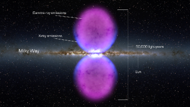
Figure 1: A gamma - X image of the Fermi bubbles in 2010 as given by the NASA.

A digitalization of the above advancing surface is reported in Figure 2 as a 2D section. This allows to fix the observed radii to be inserted in equation (20).

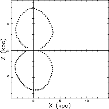
Figure 2: A section of the Fermi bubbles digitalized by the author.

The actual shape of the bubbles in galactic coordinates is shown in Figure 3 and 15 of [4] and Figure 30 and Table 3 of by [39].

4.3 The two models of reference

The thermal model is outlined in Section 3.1 and Figure 3 reports the numerical solution as a cut in the $x-z$ plane.

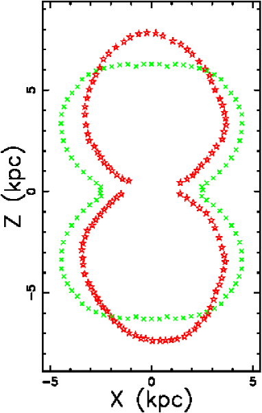
Figure 3: Section of the Fermi bubbles in the $x-z$ plane with a thermal model (green points) and observed profile (red stars). The bursting parameters $N^{*}$= 113000, $z_{\mathrm{OB}}$=0 pc, $E_{51}$=1, $t_{0}=0.036\,10^{7}\,yr$ when $t=90\,10^{7}yr$ give $\epsilon_{\mathrm{obs}}=73.34\%$.

The cold recursive model is outlined in Section 3.2 and Figure 4 reports the numerical solution as a cut in the $x-z$ plane.

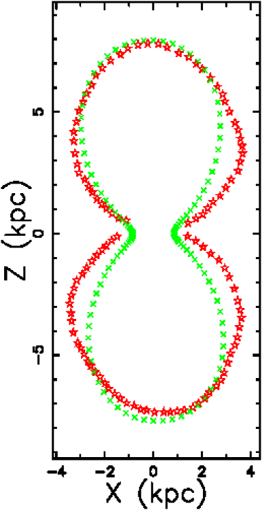
Figure 4: Section of the Fermi bubbles in the $x-z$ plane with the cold recursive model (green points) and observed profile (red stars). The bursting parameters $N^{*}$= 79000, $z_{\mathrm{OB}}$=2 pc, $t_{0}=0.013\,10^{7}$ yr and $E_{51}$=1 gives $r_{0}=90.47$ pc and $v_{0}\,=391.03$ km s^-1. On inserting $h=90$ pc, $t=13.6\,10^{7}$ yr the reliability is $\epsilon_{\mathrm{obs}}=84.70\%$.

4.4 The inverse square model

The inverse square model is outlined in Section 3.3 and Figure 5 reports the numerical solution as a cut in the $x-z$ plane.

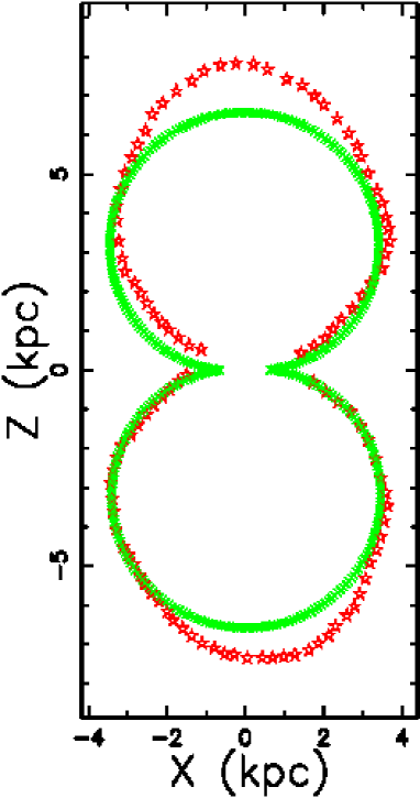
Figure 5: Section of the Fermi bubbles in the $x-z$ plane with the inverse square model (green points) and observed profile (red stars). The parameters are reported in Table 1 and the reliability is $\epsilon_{\mathrm{obs}}=90.71\%$.

A rotation around the $z$-axis of the above theoretical section allows building a 3D surface, see Figure 6.

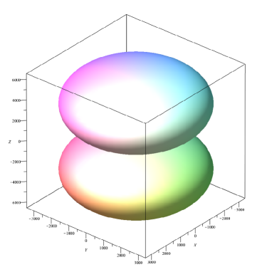
Figure 6: 3D surface of the Fermi bubbles with parameters as in Table 1, inverse square profile. The three Euler angles are $\Theta=40$, $\Phi=60$ and $\Psi=60$.

The temporal evolution of the advancing surface is reported in Figure 7 and a comparison should be done with Fig. 6 in [40].

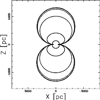
Figure 7: Sections of the Fermi bubbles as function of time with parameters as in Table 1. The time of each section is 0.0189$\,10^{7}\,yr$, 0.059$\,10^{7}\,yr$, 0.189$\,10^{7}\,yr$, 0.6$\,10^{7}\,yr$, 1.89 $\,10^{7}\,yr$, and 6$\,10^{7}\,yr$.

5 Theory of the image

This section reviews the transfer equation and reports a new analytical result for the intensity of radiation in an elliptical framework in the non-thermal/thermal case. A numerical model for the image formation of the Fermi bubbles is reported.

5.1 The transfer equation

The transfer equation in the presence of emission only in the case of optically thin layer is

$$j_{\nu}\rho=KC(s)\quad,$$ (21)

where $K$ is a constant, $j_{\nu}$ is the emission coefficient, the index $\nu$ denotes the frequency of emission and $C(s)$ is the number density of particles, see for example [41]. As an example the synchrotron emission, as described in sec. 4 of [42], is often used in order to model the radiation from a SNR, see for example [43, 44, 45]. According to the above equation the increase in intensity is proportional to the number density integrated along the line of sight, which for constant density, gives

$$I_{\nu}=K^{\prime}\times l\quad,$$ (22)

where $K^{\prime}$ is a constant and $l$ is the length along the line of sight interested in the emission; in the case of synchrotron emission see formula (1.175) in [46].

5.2 Analytical non thermal model

A real ellipsoid, see [47], represents a first approximation of the Fermi bubbles, see [38], and has equation

$$\frac{z^{2}}{a^{2}}+\frac{x^{2}}{b^{2}}+\frac{y^{2}}{d^{2}}=1\quad,$$ (23)

in which the polar axis of the Galaxy is the z-axis. Figure 8 reports the astrophysical application of the ellipsoid in which due to the symmetry about the azimuthal angle $b=d$.

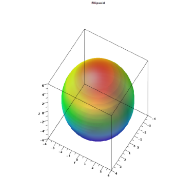
Figure 8: Fermi bubbles approximated by an ellipsoid when $a=6\,kpc,b=4\,kpcandd=4\,kpc$.

We are interested in the section of the ellipsoid $y=0$ which is defined by the following external ellipse

$$\frac{z^{2}}{a^{2}}+\frac{x^{2}}{b^{2}}=1\quad.$$ (24)

We assume that the emission takes place in a thin layer comprised between the external ellipse and the internal ellipse defined by

$$\frac{z^{2}}{(a-c)^{2}}+\frac{x^{2}}{(b-c)^{2}}=1\quad,$$ (25)

see Figure 9.

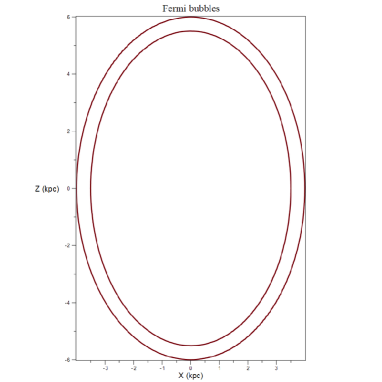
Figure 9: Internal and external ellipses when $a=6\,kpc$,$b=4\,kpc$ and $c=\frac{a}{12}\,kpc$.

We therefore assume that the number density $C$ is constant and in particular rises from 0 at (0,a) to a maximum value $C_{m}$, remains constant up to (0,a-c) and then falls again to 0. The length of sight, when the observer is situated at the infinity of the $x$-axis, is the locus parallel to the $x$-axis which crosses the position $z$ in a Cartesian $x-z$ plane and terminates at the external ellipse. The locus length is

$$l_{I}=2\,{\frac{\sqrt{{a}^{2}-{z}^{2}}b}{a}}$$ (26)

$$when\quad(a-c)\leq z<a$$

$$l_{II}=2\,{\frac{\sqrt{{a}^{2}-{z}^{2}}b}{a}}-2\,{\frac{\sqrt{{a}^{2}-2\,ac+{c}^{2}-{z}^{2}}\left(b-c\right)}{a-c}}$$ (27)

$$when\quad 0\leq z<(a-c)\quad.$$

In the case of optically thin medium, according to equation (22), the intensity is split in two cases

$$I_{I}(z;a,b)=I_{m}\times 2\,{\frac{\sqrt{{a}^{2}-{z}^{2}}b}{a}}$$ (28)

$$when\quad(a-c)\leq z<a$$

$$I_{II}(z;a,,c)=I_{m}\times\Big{(}2\,{\frac{\sqrt{{a}^{2}-{z}^{2}}b}{a}}-2\,{\frac{\sqrt{{a}^{2}-2\,ac+{c}^{2}-{z}^{2}}\left(b-c\right)}{a-c}}\Big{)}$$ (29)

$$when\quad 0\leq z<(a-c)\quad,$$

where $I_{m}$ is a constant which allows to compare the theoretical intensity with the observed one. A typical profile in intensity along the z-axis is reported in Figure 10.

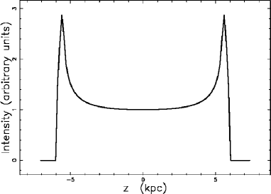
Figure 10: The intensity profile along the z-axis when when $a=6\,kpc$,$b=4\,kpc$, $c=\frac{a}{12}\,kpc$ and $I_{m}$=1.

The ratio, $r$, between the theoretical intensity at the maximum, $(z=a-c)$, and at the minimum, ($z=0$), is given by

$$\frac{I_{I}(z=a-c)}{I_{II}(z=0)}=r={\frac{\sqrt{2\,a-c}b}{\sqrt{c}a}}\quad.$$ (30)

As an example the values $a=6\,kpc$,$b=4\,kpc$, $c=\frac{a}{12}\,kpc$ gives $r=3.19$. The knowledge of the above ratio from the observations allows to deduce $c$ once $a$ and $b$ are given by the observed morphology

$$c=2\,{\frac{a{b}^{2}}{{a}^{2}{r}^{2}+{b}^{2}}}\quad.$$ (31)

As an example in the inner regions of the northeast Fermi bubble we have $r=2$, see [6], which coupled with $a=6\,kpc$ and $b=4\,kpc$ gives $c=1.2\,kpc$. The above value is an important astrophysical result because we have found the dimension of the advancing thin layer.

5.3 Analytical thermal model

A thermal model for the image is characterized by a constant temperature in the internal region of the advancing section which is approximated by an ellipse, see equation (24). We therefore assume that the number density $C$ is constant and in particular rises from 0 at (0,a) to a maximum value $C_{m}$, remains constant up to (0,-a) and then falls again to 0. The length of sight, when the observer is situated at the infinity of the $x$-axis, is the locus parallel to the $x$-axis which crosses the position $z$ in a Cartesian $x-z$ plane and terminates at the external ellipse in the point (0,a). The locus length is

$$l=2\,{\frac{\sqrt{{a}^{2}-{z}^{2}}b}{a}}\quad;-a\leq z<a\quad.$$ (32)

The number density $C_{m}$ is constant in the ellipse and therefore the intensity of radiation is

$$I(z;a,b,I_{m})=I_{m}\times 2\,{\frac{\sqrt{{a}^{2}-{z}^{2}}b}{a}}\quad;-a\leq z<a\quad.$$ (33)

A typical profile in intensity along the z-axis for the thermal model is reported in Figure 11.

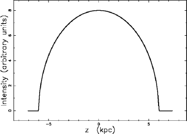
Figure 11: The intensity profile along the z-axis for the thermal model when $a=6\,kpc$, $b=4\,kpc$ and $I_{m}$=1.

5.4 Numerical model

The source of luminosity is assumed here to be the flux of kinetic energy, $L_{m}$,

$$L_{m}=\frac{1}{2}\rho AV^{3}\quad,$$ (34)

where $A$ is the considered area, $V$ the velocity and $\rho$ the density, see formula (A28) in [48]. In our case $A=R^{2}\Delta\Omega$, where $\Delta\Omega$ is the considered solid angle along the chosen direction. The observed luminosity along a given direction can be expressed as

$$L=\epsilon L_{m}\quad,$$ (35)

where $\epsilon$ is a constant of conversion from the mechanical luminosity to the observed luminosity. A numerical algorithm which allows us to build a complex image is outlined in Section 4.1 of [49] and the orientation of the object is characterized by the Euler angles $(\Phi,\Theta,\Psi)$ The threshold intensity can be parametrized to $I_{max}$, the maximum value of intensity characterizing the map. The image of the Fermi bubbles is shown in Figure 12 and the introduction of a threshold intensity is visualized in Figure 13.

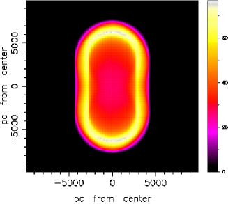
Figure 12: Map of the theoretical intensity of the Fermi bubbles for the inverse square model with parameters as in Table 1. The three Euler angles characterizing the orientation are $\Phi$=0^∘, $\Theta$=90 ^∘ and $\Psi$=90 ^∘.

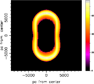
Figure 13: Map of the theoretical intensity of the Fermi bubbles as in Figure 12. In this map $I_{tr}=I_{max}/2$.

6 Conclusions

Law of motion We have compared two existing models for the temporal evolution of the Fermi bubbles, a thermal model, see Section 3.1, and an autogravitating model, see Section 3.2, with a new model which conserves the momentum in presence of an inverse square law for the density of the ISM. The best result is obtained by the inverse square model which produces a reliability of $\epsilon_{\mathrm{obs}}=90.71\%$ for the expanding radius in respect to a digitalized section of the Fermi bubbles. A semi-analytical law of motion as function of polar angle and time is derived for the inverse square model, see equation (17).

Formation of the image An analytical cut for the intensity of radiation along the z-axis is derived in the framework of advancing surface characterized by an internal and an external ellipses. The analytical cut in theoretical intensity presents a characteristic ”U” shape which has a maximum in the external ring and a minimum at the center, see equation (5.2). The presence of a hole in the intensity of radiation in the central region of the elliptical Fermi bubbles is also confirmed by a numerical algorithm for the image formation, see Figure 13. The theoretical prediction of a hole in the intensity map explains the decrease in intensity for the 0.3 kev plasma by  = $50\%$ toward the central region of the northeast Fermi bubble, see [6]. The intensity of radiation for the thermal model conversely presents a maximum of the intensity at the center of the elliptical Fermi bubble, see equation (33) and this theoretical prediction does not agree with the above observations.

References

- [1] Heiles C 1979 H I shells and supershells ApJ 229, 533
- [2] Pikel’Ner S B 1968 Interaction of Stellar Wind with Diffuse Nebulae Astrophys. Lett. 2, 97
- [3] Weaver R, McCray R, Castor J, Shapiro P and Moore R 1977 Interstellar bubbles. II - Structure and evolution ApJ 218, 377
- [4] Su M, Slatyer T R and Finkbeiner D P 2010 Giant Gamma-ray Bubbles from Fermi-LAT: Active Galactic Nucleus Activity or Bipolar Galactic Wind? ApJ 724, 1044 (Preprint 1005.5480)
- [5] Jones D I, Crocker R M, Reich W and et al 2012 Magnetic Substructure in the Northern Fermi Bubble Revealed by Polarized Microwave Emission ApJ 747 L12 (Preprint 1201.4491)
- [6] Kataoka J, Tahara M, Totani T and et al 2013 Suzaku Observations of the Diffuse X-Ray Emission across the Fermi Bubbles’ Edges ApJ 779 57 (Preprint 1310.3553)
- [7] Tahara M, Kataoka J, Takeuchi Y and et al 2015 Suzaku X-Ray Observations of the Fermi Bubbles: Northernmost Cap and Southeast Claw Discovered With MAXI-SSC ApJ 802 91 (Preprint 1501.04405)
- [8] Kataoka J, Tahara M, Totani T and et al 2015 Global Structure of Isothermal Diffuse X-Ray Emission along the Fermi Bubbles ApJ 807 77 (Preprint 1505.05936)
- [9] Fox A J, Bordoloi R, Savage B D and et al 2015 Probing the Fermi Bubbles in Ultraviolet Absorption: A Spectroscopic Signature of the Milky Way’s Biconical Nuclear Outflow ApJ 799 L7 (Preprint 1412.1480)
- [10] Bordoloi R, Fox A J, Lockman F J and et al 2017 Mapping the Nuclear Outflow of the Milky Way: Studying the Kinematics and Spatial Extent of the Northern Fermi Bubble ApJ 834 191 (Preprint 1612.01578)
- [11] Abeysekara A U, Albert A, Alfaro R and et al 2017 Search for Very High-energy Gamma Rays from the Northern Fermi Bubble Region with HAWC ApJ 842 85 (Preprint 1703.01344)
- [12] Cheng K S, Chernyshov D O, Dogiel V A and et al 2011 Origin of the Fermi Bubble ApJ 731 L17 (Preprint 1103.1002)
- [13] Yang H Y K, Ruszkowski M, Ricker P M and et al 2012 The Fermi Bubbles: Supersonic Active Galactic Nucleus Jets with Anisotropic Cosmic-Ray Diffusion ApJ 761 185 (Preprint 1207.4185)
- [14] Fujita Y, Ohira Y and Yamazaki R 2013 The Fermi Bubbles as a Scaled-up Version of Supernova Remnants ApJ 775 L20 (Preprint 1308.5228)
- [15] Thoudam S 2013 Fermi Bubble -Rays as a Result of Diffusive Injection of Galactic Cosmic Rays ApJ 778 L20 (Preprint 1304.6972)
- [16] Fujita Y, Ohira Y and Yamazaki R 2014 A Hadronic-leptonic Model for the Fermi Bubbles: Cosmic-Rays in the Galactic Halo and Radio Emission ApJ 789 67 (Preprint 1405.5214)
- [17] Cheng K S, Chernyshov D O, Dogiel V A and Ko C M 2015 Multi-wavelength Emission from the Fermi Bubble. II. Secondary Electrons and the Hadronic Model of the Bubble ApJ 799 112 (Preprint 1411.6395)
- [18] Sasaki K, Asano K and Terasawa T 2015 Time-dependent Stochastic Acceleration Model for Fermi Bubbles ApJ 814 93 (Preprint 1510.02869)
- [19] Keshet U and Gurwich I 2017 Fermi Bubble Edges: Spectrum and Diffusion Function ApJ 840 7 (Preprint 1611.04190)
- [20] Crocker R M, Bicknell G V, Carretti E and et al 2014 Steady-state Hadronic Gamma-Ray Emission from 100-Myr-Old Fermi Bubbles ApJ 791 L20 (Preprint 1312.0692)
- [21] Lockman F J 1984 The H I halo in the inner galaxy ApJ 283, 90
- [22] Dickey J M and Lockman F J 1990 H I in the Galaxy ARA&A 28, 215
- [23] Bisnovatyi-Kogan G S and Silich S A 1995 Shock-wave propagation in the nonuniform interstellar medium Rev. Mod. Phys. 67, 661
- [24] Zhu H, Tian W, Li A and Zhang M 2017 The gas-to-extinction ratio and the gas distribution in the Galaxy MNRAS 471, 3494 (Preprint 1706.07109)
- [25] Spitzer Jr L 1942 The Dynamics of the Interstellar Medium. III. Galactic Distribution. ApJ 95, 329
- [26] Rohlfs K, ed 1977 Lectures on density wave theory vol 69 of Lecture Notes in Physics, Berlin Springer Verlag
- [27] Bertin G 2000 Dynamics of Galaxies (Cambridge: Cambridge University Press.)
- [28] Padmanabhan P 2002 Theoretical astrophysics. Vol. III: Galaxies and Cosmology (Cambridge, UK: Cambridge University Press)
- [29] McCray R A 1987 Coronal interstellar gas and supernova remnants in A Dalgarno & D Layzer, ed, Spectroscopy of Astrophysical Plasmas (Cambridge: Cambridge University Press. ) pp 255–278
- [30] Dyson, J E and Williams, D A 1997 The physics of the interstellar medium (Bristol: Institute of Physics Publishing)
- [31] McCray R and Kafatos M 1987 Supershells and propagating star formation ApJ 317, 190
- [32] Zaninetti L 2004 On the Shape of Superbubbles Evolving in the Galactic Plane PASJ 56, 1067
- [33] Zaninetti L 2012 Evolution of superbubbles in a self-gravitating disc Monthly Notices of the Royal Astronomical Society 425, 2343 ISSN 1365-2966
- [34] Padé H 1892 Sur la représentation approchée d’une fonction par des fractions rationnelles Ann. Sci. Ecole Norm. Sup. 9, 193
- [35] Olver F W J e, Lozier D W e, Boisvert R F e and Clark C W e 2010 NIST handbook of mathematical functions. (Cambridge: Cambridge University Press. )
- [36] Baker G 1975 Essentials of Padé approximants (New York: Academic Press)
- [37] Baker G A and Graves-Morris P R 1996 Padé approximants vol 59 (Cambridge: Cambridge University Press)
- [38] Miller M J and Bregman J N 2016 The Interaction of the Fermi Bubbles with the Milky Way’s Hot Gas Halo ApJ 829 9 (Preprint 1607.04906)
- [39] Ackermann M, Albert A, Atwood W B and et al 2014 The Spectrum and Morphology of the Fermi Bubbles ApJ 793 64 (Preprint 1407.7905)
- [40] Sofue Y 2017 Giant H i hole inside the 3 kpc ring and the North Polar Spur-The Galactic crater PASJ 69 L8 (Preprint 1706.08771)
- [41] Rybicki G and Lightman A 1991 Radiative Processes in Astrophysics (New-York: Wiley-Interscience)
- [42] Schlickeiser R 2002 Cosmic ray astrophysics (Berlin: Springer)
- [43] Yamazaki R, Ohira Y, Sawada M and Bamba A 2014 Synchrotron X-ray diagnostics of cutoff shape of nonthermal electron spectrum at young supernova remnants Research in Astronomy and Astrophysics 14 165-178 (Preprint 1301.7499)
- [44] Tran A, Williams B J, Petre R, Ressler S M and Reynolds S P 2015 Energy Dependence of Synchrotron X-Ray Rims in Tycho’s Supernova Remnant ApJ 812 101 (Preprint 1509.00877)
- [45] Katsuda S, Acero F, Tominaga N, Fukui Y, Hiraga J S, Koyama K, Lee S H, Mori K, Nagataki S, Ohira Y, Petre R, Sano H, Takeuchi Y, Tamagawa T, Tsuji N, Tsunemi H and Uchiyama Y 2015 Evidence for Thermal X-Ray Line Emission from the Synchrotron-dominated Supernova Remnant RX J1713.7-3946 ApJ 814 29 (Preprint 1510.04025)
- [46] Lang K R 1999 Astrophysical formulae. (Third Edition) (New York: Springer)
- [47] Zwillinger D 2018 CRC Standard Mathematical Tables and Formulas, 33rd Edition Advances in Applied Mathematics (New York: CRC Press) ISBN 9781351651004 URL https://books.google.it/books?id=yyhFDwAAQBAJ
- [48] De Young D S 2002 The physics of extragalactic radio sources (Chicago: University of Chicago Press)
- [49] Zaninetti L 2013 Three dimensional evolution of sn 1987a in a self-gravitating disk International Journal of Astronomy and Astrophysics 3, 93