An Input-Output Approach to
Structured Stochastic Uncertainty in Continuous Time

Abstract

We consider the continuous-time setting of linear time-invariant (LTI) systems in feedback with multiplicative stochastic uncertainties. The objective of the paper is to characterize the conditions of Mean-Square Stability (MSS) using a purely input-output approach, i.e. without having to resort to state space realizations. This has the advantage of encompassing a wider class of models (such as infinite dimensional systems and systems with delays). The input-output approach leads to uncovering new tools such as stochastic block diagrams that have an intimate connection with the more general Stochastic Integral Equations (SIE), rather than Stochastic Differential Equations (SDE). Various stochastic interpretations are considered, such as Itō and Stratonovich, and block diagram conversion schemes between different interpretations are devised. The MSS conditions are given in terms of the spectral radius of a matrix operator that takes different forms when different stochastic interpretations are considered.

I INTRODUCTION

Linear Time-Invariant (LTI) systems with stochastic disturbances is a powerful modeling technique that is used to analyze and control a large class of physical systems. While additive disturbances are most commonly used to model process and measurement noise in a system, multiplicative disturbances are often necessary to model stochastic uncertainties in the system parameters (such as coefficients in dynamical equations). LTI systems driven by additive stochastic processes are more common in the literature; whereas simultaneous additive and multiplicative disturbances are relatively less addressed. The present paper develops a methodology to study the mean-square stability of continuous-time systems with both additive and multiplicative disturbances, while adopting different stochastic interpretations (such as Itō and Stratonovich).

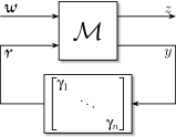
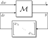
(a) White Process Representation	(b) Wiener Process Representation

Figure 1: The general continuous-time setting of linear systems with both additive and multiplicative stochastic disturbances. Both block diagrams describe the same setting, given in (I) and (I), using white processes (to the left) and Wiener processes (to the right), respectively. The LTI system $\mathcal{M}$ is in feedback with multiplicative stochastic gains represented here as a diagonal matrix. In Figure (a), w is an additive stationary white process, while $\upgamma_{1},\cdots,\upgamma_{n}$ are multiplicative stationary white processes. In Figure (b), $dw$ represents the differential of an additive Wiener process, while $d\gamma_{1},\cdots,d\gamma_{n}$ represent the differentials of (possibly correlated) Wiener processes that enter the dynamics multiplicatively. The signal $z$ represents an output whose variance quantifies a performance measure.

The general setting we consider in this paper is the continuous-time analog of that presented in [1] and is depicted in Figure 1(a). An LTI system is in feedback with stochastic gains $\upgamma_{1}(t),...\upgamma_{n}(t)$, that are assumed to be “white” in time (i.e. temporally independent) but possibly mutually correlated. Another set of stochastic disturbances are represented by the vector-valued signal w which is also assumed to be white but enters the dynamics additively. The signal $z$ is an output whose variance quantifies a performance measure. The feedback term is then a diagonal matrix with the individual gains $\{\upgamma_{i}\}$ appearing on the diagonal. Such gains are commonly referred to as structured uncertainties. Note that if the gains are deterministic (but uncertain), we obtain the general setting considered in the robust control literature (e.g. [2]). The main objective of the present paper is to derive the necessary conditions of Mean-Square Stability (MSS) for systems taking the form of Figure 1(a). The treatment is carried out using a purely input-output approach (i.e. without giving $\mathcal{M}$ a state space realization). This has the advantage of encompassing a wider class of models $\mathcal{M}$ (e.g. infinite dimensional systems).

In a discrete-time setting, there is no ambiguity of defining white (i.e. temporally independent) signals. However, in a continuous-time setting, technical issues arise because white signals are not mathematically well defined when they enter the dynamics multiplicatively. Hence, the block diagram in Figure 1(a) is only used to pose the problem setup in an analogous fashion to the discrete-time setting in [1], but at the cost of abandoning mathematical rigor. In fact, the equations describing Figure 1 can be written using the white processes w and $\{\upgamma_{i}\}$ as

$$\begin{bmatrix}z\\ y\end{bmatrix} =\mathcal{M}\begin{bmatrix}\text{\Fontauri w}\\ \text{\Fontauri r}\end{bmatrix}\Leftrightarrow\begin{bmatrix}z(t)\\ y(t)\end{bmatrix}={\int_{0}^{t}}M(t-\tau)\begin{bmatrix}\text{\Fontauri w}(\tau)\\ \text{\Fontauri r}(\tau)\end{bmatrix}d\tau$$

$$\text{\Fontauri r}(t) =\mathcal{D}\big{(}\boldsymbol{\upgamma}(t)\big{)}y(t),$$ (1)

where $M$ is the impulse response of $\mathcal{M}$, and $\mathcal{D}\big{(}\boldsymbol{\upgamma}(t)\big{)}$ is a diagonal matrix whose elements are equal to those of $\boldsymbol{\upgamma}(t):=\begin{bmatrix}\upgamma_{1}(t)&\cdots&\upgamma_{n}(t)\end{bmatrix}^{*}$. To resort back to mathematical rigor, we think of the white processes w and $\{\upgamma_{i}\}$ as the formal derivatives of Wiener processes (or Brownian motion) that are mathematically well defined [3]. More precisely, define

$$\upgamma_{i}(t):=\frac{d\gamma_{i}(t)}{dt};\quad\text{\Fontauri w}(t):=\frac{dw(t)}{dt};\quad\text{\Fontauri r}(t):=\frac{dr(t)}{dt},$$ (2)

such that $\boldsymbol{\gamma}(t):=\begin{bmatrix}\gamma_{1}(t)&\cdots&\gamma_{n}(t)\end{bmatrix}^{*}$ and $w(t)$ represent nonstandard, vector-valued Wiener processes (i.e. their covariances do not have to be the identity matrix). Furthermore, $r(t)$ will be shown (Section VII-A3) to have temporally independent increments when $\mathcal{M}$ is causal and the Itō interpretation is adopted. Hence, the equations can be rewritten using differential forms as

$$\begin{bmatrix}z\\ y\end{bmatrix}=\mathcal{M}\begin{bmatrix}dw\\ dr\end{bmatrix}\Leftrightarrow\begin{bmatrix}z(t)\\ y(t)\end{bmatrix}={\int_{0}^{t}}M(t-\tau)\begin{bmatrix}dw(\tau)\\ dr(\tau)\end{bmatrix}$$

$$dr(t)=\mathcal{D}\big{(}d{\boldsymbol{\gamma}}(t)\big{)}y(t).$$ (3)

These equations are now mathematically well defined when given some desired interpretation such as in the sense of Itō or Stratonovich. It will be shown in Section IV-B that different interpretations produce different conditions of MSS.

We should note the other common and related models in the literature which are usually done in a state space setting and can be represented as Stochastic Differential Equations (SDEs). One such model is a linear system with a random “A matrix” such as

$$\dot{x}(t)=A(t)x(t)+B\text{\Fontauri w}(t),$$ (4)

where $A(t)$ is a matrix-valued stochastic process independent of $\{x(\tau),\tau\leq t\}$. One can always rewrite $A(t)$ in terms of scalar-valued stochastic processes so that

$$\dot{x}(t)=\big{(}A_{0}+\upgamma_{1}(t)A_{1}+\cdots+\upgamma_{n}(t)A_{n}\big{)}x(t)+B\text{\Fontauri w}(t).$$

If the matrices $A_{1},\ldots,A_{n}$ are all of rank 1 (e.g. $A_{i}=b_{i}c_{i}$, for column and row vectors $b_{i}$, $c_{i}$ respectively, $i=1,\ldots,n$), then it is well-known [2] that the model (4) can always be reconfigured like the block diagram of Figure 1(a) by setting

$$\mathcal{M}~{}=~{}\left[\begin{array}[]{c|cc}A_{0}&B&B_{0}\\ \hline\cr C&0&0\\ C_{0}&0&0\end{array}\right],$$

where $B_{0}:=\begin{bmatrix}b_{1}&\cdots&b_{n}\end{bmatrix}$ and $C_{0}:=\begin{bmatrix}c_{1}^{*}&\cdots&c_{n}^{*}\end{bmatrix}^{*}$. In the example above, we have chosen $z=Cx$. If the matrices $\{A_{i}\}_{i=1}^{n}$ are not rank one, it is still possible to reconfigure (4) into a diagram like Figure 1(a), but with the perturbation blocks being “repeated” [4].

When the processes $\{\upgamma_{i}\}$ and w are “white” in time, we resort to the configuration of Figure 1(b) to express the stochastic disturbances in terms of Wiener processes. Exploiting (2) yields

$$\mathcal{M}: \left\{\begin{aligned} dx(t)&=A_{0}x(t)dt+B_{0}dr(t)+Bdw(t)\\ y(t)&=C_{0}x(t)\\ z(t)&=Cx(t)\end{aligned}\right.$$ (5)

$$dr(t)=\mathcal{D}\big{(}d\boldsymbol{\gamma}(t)\big{)}y(t).$$ (6)

Equations (5) and (6) describe the block diagram of Figure 1(b) when $\mathcal{M}$ is given as a state space realization. In fact, the impulse response can be easily calculated to be

$$M(t):=\begin{bmatrix}C\\ C_{0}\end{bmatrix}e^{A_{0}t}\begin{bmatrix}B&B_{0}\end{bmatrix},$$

thus showing that models like those given in (4) are a special case of the purely input-output approach that we consider in this paper. On a side note, observe that the underlying stochastic dynamics of the state $x$ in (5) and (6) can be rewritten in a single SDE, that involves both additive and multiplicative disturbances, as

$$dx(t)=A_{0}x(t)dt+B_{0}\mathcal{D}\big{(}Cx(t)\big{)}d\boldsymbol{\gamma}(t)+Bdw(t).$$ (7)

Particularly, [5] studied SDEs having the form of (7) interpreted in the sense of Itō, where $B=0$ (i.e. no additive noise) and $\boldsymbol{\gamma}$ is “spatially uncorrelated”, i.e. $\mathbb{E}[\gamma_{i}\gamma_{j}]=0,\forall i\neq j$.

Our goal in this paper is to extend the machinery developed in [1] to provide a rather elementary, and purely input-output treatment and derivation of the necessary and sufficient conditions of MSS for systems like that of Figure 1. Furthermore, our treatment covers both Itō and Stratonovich interpretations. It is shown that the conditions of MSS can be stated in terms of the spectral radius of a finite dimensional linear operator defined in Section IV-B. It is also shown that this operator takes different forms when different stochastic interpretations are prescribed (such as Itō or Stratonovich).

The paper is organized as follows. First we provide some useful definitions and notation. Then, in Section III, we give a precise formulation of the problem statement by setting up a general “stochastic block diagram” and describing the underlying assumptions. In Section IV, we present the main results of the paper that can be divided into two parts. The first part shows a block diagram conversion scheme from Stratonovich to Itō interpretations, and the second part states the conditions of mean-square stability. The special cases of state space realizations are then treated in Section V. Sections VI and VII provide the detailed derivations that explain the results. Finally, we conclude in Section VIII.

II Preliminaries and Notation

All the signals considered in this paper are defined on the semi-infinite, continuous-time interval $\mathbb{R}^{+}:=[0,+\infty)$. The dynamical systems considered are maps between various signal spaces over the time interval $\mathbb{R}^{+}$. Unless stated otherwise, all stochastic processes in this paper are random vector-valued functions of (continuous) time.

Notation Summary

II-1 Variance & Covariance Matrix of a Signal

If $v$ is a stochastic signal, then its instantaneous variance and covariance matrix are denoted by the lowercase and uppercase bold letters respectively

$$\mathbf{v}(t):=\mathbb{E}\left[v^{*}(t)v(t)\right]\quad\text{and}\quad\mathbf{V}(t):=\mathbb{E}\left[v(t)v^{*}(t)\right],$$

where $v^{*}$ denotes the transpose of $v$. The entries of $\mathbf{V}(t)$ are the mutual correlations of the vector $v(t)$, and are sometimes referred to as spatial correlations. Note that $\text{tr}\left(\mathbf{V}(t)\right)=\mathbf{v}(t)$.

II-2 Variance & Covariance Matrix of a Differential Signal

If the differential $du$ of a stochastic signal $u$ appears in a stochastic block diagram (see Figure 2 for example), its instantaneous variance and covariance are represented as

$$\mathbb{E}\left[du^{*}(t)du(t)\right]:=\mathbf{u}(t)dt\quad\text{and}\quad\mathbb{E}\left[du(t)du^{*}(t)\right]:=\mathbf{U}(t)dt,$$

respectively. This is a compact (differential) notation for

$$\mathbb{E}\left[u^{*}(t)u(t)\right]:=\int_{0}^{t}\mathbf{u}(\tau)d\tau;\quad\mathbb{E}\left[u(t)u^{*}(t)\right]:=\int_{0}^{t}\mathbf{U}(\tau)d\tau.$$

II-3 Steady State Variance & Covariance Matrix

The asymptotic limits of the instantaneous variance and covariance matrix, when they exist, are denoted by an overbar, i.e.

$$\bar{\mathbf{u}}:=\lim_{t\to\infty}\mathbf{u}(t)\quad\text{and}\quad\bar{\mathbf{U}}:=\lim_{t\to\infty}\mathbf{U}(t).$$

II-4 Second Order Process

A process $v$ is termed second order if the entries of its covariance matrix, $\mathbf{V}(t)$, are finite for each $t\in\mathbb{R}^{+}$.

II-5 Probability Space

Let $(\Omega,\mathcal{F},p)$ be a complete probability space with $\Omega$ being the sample space, $\mathcal{F}$ the associated $\sigma-$algebra and $p$ the probability measure. Let $L_{2}(p)$ denote the space of vector-valued random variables with finite second order moments. Note that $L_{2}(p)$ is a Hilbert space.

II-6 Equalities & Limits in the Mean-Square Sense

Two stochastic processes $x$ and $y$ are said to be equal in the mean-square sense if $\mathbb{E}\left[\left|\left|x-y\right|\right|^{2}\right]=0$, where throughout the paper $\left|\left|.\right|\right|$ denotes the $\ell^{2}-\text{norm}$ for vectors and the spectral norm for matrices.

A sequence of second order stochastic processes, $\{x_{N}\}$, is said to converge to $\bar{x}\in L_{2}(p)$ in the mean-square sense iff $\lim_{N\to\infty}\left|\left|x_{N}-\bar{x}\right|\right|^{2}=0$.

II-7 White Process

A stochastic process $\upgamma$ is termed white if it is uncorrelated at any two distinct times, i.e. $\mathbb{E}\left[\upgamma(t)\upgamma^{*}(\tau)\right]=\mathbf{\Gamma}\delta(t-\tau)$, where $\delta$ is the Dirac delta function. Note that in the present context, a white process $\upgamma$ may still have spatial correlations, i.e. its instantaneous covariance matrix $\mathbf{\Gamma}$ need not be the identity.

II-8 Vector-Valued Wiener Process

In a continuous-time setting, calculus operations on a white process entering the dynamics multiplicatively are not mathematically well defined. Hence, it is useful to represent a white process as the formal derivative of a Wiener process, i.e. $\upgamma(t):=\frac{d\boldsymbol{\gamma}(t)}{dt}$, where $\boldsymbol{\gamma}$ is a zero-mean, vector-valued Wiener process with an instantaneous covariance matrix $\mathbb{E}\left[\boldsymbol{\gamma}(t)\boldsymbol{\gamma}^{*}(t)\right]=\mathbf{\Gamma}t$. This can be equivalently written in differential form as $\mathbb{E}\left[d\boldsymbol{\gamma}(t)d\boldsymbol{\gamma}^{*}(t)\right]=\mathbf{\Gamma}dt$. Note that $\boldsymbol{\gamma}$ is said to have temporally independent increments, i.e. its differentials $\big{(}d\boldsymbol{\gamma}(t),d\boldsymbol{\gamma}(\tau)\big{)}$ are independent when $t\neq\tau$.

II-9 Partitions of Time Intervals

Let $\mathcal{P}_{N}[0,t]$ denote an arbitrary partition of the time interval $[0,t]$ into $N$ subintervals $[t_{k},t_{k+1}]$ for $k=0,1,\cdots,N-1$, such that $0=t_{0}<t_{1}<\cdots<t_{N}=t$. The partition step-size is denoted by $\Delta_{k}:=t_{k+1}-t_{k}$ and the norm of the partition $\mathcal{P}_{N}[0,t]$ is denoted by the bold letter $\mathbf{\Delta}$ defined as $\mathbf{\Delta}:=||\mathcal{P}_{N}[0,t]||=\sup_{k}\Delta_{k}.$ Note that $\lim_{N\to\infty}{\mathbf{\Delta}}=0$.

II-10 Notation for Signals and Increments on $\mathcal{P}_{N}[0,t]$

With slight abuse of notation, a continuous-time stochastic signal $\{u(\tau),0\leq\tau\leq t\}$ is represented at node $t_{k}$ of the partition $\mathcal{P}_{N}[0,t]$ as $u_{k}:=u(t_{k})$ for $k=0,1,\cdots,N$. The increments of $\{u(\tau),0\leq\tau\leq t\}$ at $t_{k}$ are denoted by $\tilde{u}_{k}:=u(t_{k+1})-u(t_{k})$ for $k=0,1,\cdots,N-1$, and they represent a finite approximation of the differential form $\{du(\tau),0\leq\tau\leq t\}$.

A continuous-time stochastic process $u$ is said to have temporally independent increments if $\big{(}du(t),du(\tau)\big{)}$ are independent whenever $t\neq\tau$. This implies that, on the partition $\mathcal{P}_{N}[0,t]$, $(\tilde{u}_{k},\tilde{u}_{l})$ are independent whenever $k\neq l$.

II-11 Stochastic Integrals

Calculus operations on a Wiener process are mathematically well defined when some stochastic interpretation is prescribed (such as Itō or Stratonovich). Particularly, we distinguish Itō and Stratonovich integrals using the symbols ”$\diamond_{I}$” and ”$\diamond_{S}$”, respectively. More precisely, let $v$ be a vector-valued second order stochastic process and $\boldsymbol{\gamma}$ be a vector-valued Wiener process. If $\Gamma(t):=\mathcal{D}\big{(}\boldsymbol{\gamma}(t)\big{)}$ is a diagonal matrix whose entries are equal to those of $\boldsymbol{\gamma}(t)$, then the integral “$\int_{0}^{t}d\Gamma(\tau)v(\tau)$” may be interpreted differently using partial sums as

$$\int_{0}^{t}d\Gamma(\tau)\diamond_{I}v(\tau) :=\lim_{N\to\infty}\sum_{k=0}^{N-1}\tilde{\Gamma}_{k}v_{k}$$ (8)

$$\int_{0}^{t}d\Gamma(\tau)\diamond_{S}v(\tau) :=\lim_{N\to\infty}\sum_{k=0}^{N-1}\tilde{\Gamma}_{k}\frac{v_{k}+v_{k+1}}{2}.$$ (9)

The partial sums are constructed using a partition $\mathcal{P}_{N}[0,t]$ as described in Section II-9 and by following the notation developed in Section II-10 for signals and increments.

II-12 Quadratic Variation

The quadratic variation, at time $t$, of a stochastic process $v$ is denoted by $\langle v\rangle(t)$ and is defined using a partition $\mathcal{P}_{N}[0,t]$ as

$$\langle v\rangle(t):=\lim_{N\to\infty}\sum_{k=0}^{N-1}\left|\left|\tilde{v}_{k}\right|\right|^{2}.$$

II-13 Hadamard Product and the Diagonal Operator

For any two matrices $A$ and $B$ of the same dimensions, their Hadamard (or element-by-element) product is denoted by ${A\circ B}$. For any vector $v$ (resp. square matrix $V$), $\mathcal{D}(v)$ (resp. $\mathcal{D}(V)$) denotes a diagonal matrix whose diagonal elements are equal to $v$ (resp. diagonal entries of $V$).

III Problem Formulation

In this section, we first provide a precise definition for Mean-Square Stability (MSS) from a purely input/output approach. Then we present a “stochastic block diagram” formalism that can be given a desirable interpretation by prescribing a suitable stochastic calculus (Itō or Stratonovich).

III-A Input-Output Formulation of MSS

Let $\mathcal{M}$ be a causal LTI (MIMO) system. It is defined as a linear operator that acts on the differential of a second order stochastic signal $u$, denoted by $du$. Its action is defined by the stochastic convolution integral

$$y(t)=\big{(}\mathcal{M}du\big{)}(t)\Longleftrightarrow y(t)=\int_{0}^{t}M(t-\tau)~{}du(\tau),$$ (10)

where $M$ is a deterministic matrix-valued function denoting the impulse response of $\mathcal{M}$. Without loss of generality, zero initial conditions are assumed throughout this paper. When $u$ is zero-mean and has independent increments such that $\mathbb{E}\left[du(t)du^{*}(\tau)\right]=0~{}\forall t\neq\tau$ and $\mathbb{E}\left[du(t)du^{*}(t)\right]=\mathbf{U}(t)dt$, a standard calculation relates the input and output instantaneous covariances as

$$\mathbf{Y}(t)=\int_{0}^{t}M(t-\tau)~{}\mathbf{U}(\tau)~{}M^{*}(t-\tau)d\tau.$$ (11)

Note that (11) holds for any stochastic interpretation (eg. Itō or Stratonovich) of the stochastic integral in (10) as shown in Appendix -A. Therefore, the action of $\mathcal{M}$ as described in (10) is not given a particular stochastic interpretation throughout the paper. Unlike (10), this matrix convolution relationship is deterministic, and it is only valid when the input $du$ is temporally independent (i.e. $u$ has independent increments). Taking the trace of both sides of (11) yields

$$\mathbf{y}(t) =\text{tr}\left(\mathbf{Y}(t)\right)=\int_{0}^{t}\text{tr}\big{(}M(t-\tau)\mathbf{U}(\tau)M^{*}(t-\tau)\big{)}d\tau$$

$$=\int_{0}^{t}\text{tr}\big{(}M^{*}(t-\tau)M(t-\tau)\mathbf{U}(\tau)\big{)}d\tau$$

$$\leq\int_{0}^{t}\text{tr}\big{(}M^{*}(t-\tau)M(t-\tau)\big{)}\text{tr}\big{(}\mathbf{U}(\tau)\big{)}d\tau$$

$$\leq\int_{0}^{\infty}\text{tr}\big{(}M^{*}(t-\tau)M(t-\tau)\big{)}d\tau\sup_{0\leq\tau\leq\infty}\mathbf{u}(\tau),$$

where the first inequality holds because for any two positive semidefinite matrices $A$ and $B$, we have ${\text{tr}\left(AB\right)\leq\text{tr}\left(A\right)\text{tr}\left(B\right)}$ [6, Thm 1]. The calculation above motivates the following definition for input/output MSS when the input is temporally independent.

Definition 1

A causal LTI system $\mathcal{M}$ is Mean-Square Stable (MSS) if for each input $du$, representing the differential of a stochastic process with independent increments and uniformly bounded variance, the output process $y=\mathcal{M}du$ has a uniformly bounded variance, i.e. there exists a constant $c$ such that $\mathbf{y}(t)\leq c~{}\sup_{\tau}\mathbf{u}(\tau)$.

It is easy to check that $\mathcal{M}$ is MSS in the sense of Definition 1 if and only if $\|\mathcal{M}\|_{2}$ is finite, where $\left|\left|.\right|\right|_{2}$ denotes the $H^{2}-\text{norm}$. When MSS holds, the output covariance has a finite steady-state limit $\bar{\mathbf{Y}}$ whenever the input covariance has a finite steady-state limit $\bar{\mathbf{U}}$. From (11), it is straight forward to see that the steady-state covariances (if they exist) are related as

$$\bar{\mathbf{Y}}=\int_{0}^{\infty}M(\tau)\bar{\mathbf{U}}M^{*}(\tau)d\tau.$$ (12)

III-B Stochastic Feedback Interconnection

Consider the “stochastic block diagram” depicted in Figure 2 where the forward block represents a causal LTI system which is in feedback with multiplicative stochastic gains represented here as the differential of a diagonal matrix denoted by $d\Gamma(t)$ where

$$d\Gamma(t):=\mathcal{D}\big{(}d\boldsymbol{\gamma}(t)\big{)}\quad\text{and}\quad d\boldsymbol{\gamma}(t):=\begin{bmatrix}d\gamma_{1}(t)&\cdots&d\gamma_{n}(t)\end{bmatrix}^{*}.$$ (13)

Furthermore, a different type of stochastic disturbance enters the dynamics additively and is represented in Figure 2 as the differential of $w$.

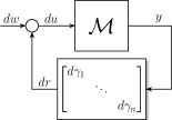
Figure 2: A continuous-time setting for a causal LTI system $\mathcal{M}$ in feedback with stochastic multiplicative gains $\{d\gamma_{i}\}$ that represent the differential forms of, possibly mutually correlated, Wiener processes. The equations describing the block diagram are given in (14).

The main objective of this paper is to investigate the MSS of Figure 2 under the following assumptions

• Assumption 1

  $\mathcal{M}$ is a causal LTI (MIMO) system whose impulse response $M$ belongs to the class $\mathcal{C}$ of deterministic, matrix-valued functions defined in Appendix -E. Note that for such $M$, $\exists$ a continuous scalar function $c_{M}$ such that $\sup\limits_{0\leq\tau\leq t}\left|\left|M(\tau)\right|\right|=c_{M}(t).$

• Assumption 2

  $\boldsymbol{\gamma}(t):=\begin{bmatrix}\gamma_{1}(t)&\cdots&\gamma_{n}(t)\end{bmatrix}^{*}$ is a zero-mean, vector-valued Wiener process with an instantaneous covariance $\mathbb{E}\left[\boldsymbol{\gamma}(t)\boldsymbol{\gamma}^{*}(t)\right]:=\mathbf{\Gamma}t$ which can be equivalently written as $\mathbb{E}\left[d\boldsymbol{\gamma}(t)d\boldsymbol{\gamma}^{*}(t)\right]=\mathbf{\Gamma}dt$ (refer to Section II-8). Note that $\mathbf{\Gamma}$ is a constant positive semidefinite matrix.

• Assumption 3

  $w$ is a zero-mean, vector-valued Wiener process with a (possibly) time-varying instantaneous covariance matrix, i.e. $\mathbb{E}\left[dw(t)dw^{*}(t)\right]=\mathbf{W}(t)dt$, where $\mathbf{W}$ is a positive semidefinite matrix whose entries remain bounded for all time. Furthermore, $\mathbf{W}$ is assumed to be monotone, i.e. if $t_{1}\leq t_{2}$ then $\mathbf{W}(t_{1})\leq\mathbf{W}(t_{2})$.

• Assumption 4

  $\boldsymbol{\gamma}$ and $w$ are uncorrelated for all time.

Throughout the paper, whenever the Stratonovich interpretation is adopted, a more restrictive assumption on $M$ is required for reasons that will become apparent in Section VI. Thus Assumption 1 is replaced by

• Assumption 1^′

  $M$ is Lipschitz continuous.

Note that the class of Lipschitz continuous functions is more restrictive than class $\mathcal{C}$ defined in Appendix -E. In fact, it is fairly straightforward to see that if $M$ is Lipschitz continuous, then $M\in\mathcal{C}$.

The equations describing the block diagram in Figure 2 can be written as

$$\left\{\begin{aligned} y(t)&=\left(\mathcal{M}du\right)(t)\\ du(t)&=dw(t)+dr(t)\\ dr(t)&=d\Gamma(t)y(t).\end{aligned}\right.$$ (14)

Note that, without prescribing a stochastic interpretation for the calculus operations on the Wiener processes $w$ and $\Gamma$, the set of equations in (14) are not sufficient to fully describe the underlying stochastic dynamics. In this paper, we consider the two most common interpretations named after Itō and Stratonovich; however, the analysis can be generalized to other interpretations as well. We encode the stochastic interpretations in (14) by rewriting them as

$$\left\{\begin{aligned} y(t)&=\left(\mathcal{M}du\right)(t)\\ du(t)&=dw(t)+dr(t)\\ dr(t)&=d\Gamma(t)\diamond y(t);\qquad\qquad\text{for}\quad\diamond=\{\diamond_{I},\diamond_{S}\},\end{aligned}\right.$$ (15)

where the last equation is the differential form of an integral equation that can be written as

$$r(t)=\int_{0}^{t}d\Gamma(\tau)\diamond y(\tau),\qquad\text{where}\quad\diamond=\{\diamond_{I},\diamond_{S}\}.$$

Refer to Section II-11 for an explanation of the different interpretations. Note that We close this section by giving a definition for MSS of the stochastic feedback system in Figure 2 by following the convention given in [7].

Definition 2

Consider the stochastic feedback interconnection in Figure 2 satisfying Assumptions 1-4. The overall feedback system is said to be MSS if all the signals in the loop, i.e. $du,dr$ and $y$ have uniformly bounded variances. More precisely, there exists a constant $c$ such that

$$\text{max}\{\left|\left|\mathbf{u}\right|\right|_{\infty},\left|\left|\mathbf{r}\right|\right|_{\infty},\left|\left|\mathbf{y}\right|\right|_{\infty}\}\leq c\left|\left|\mathbf{w}\right|\right|_{\infty}.$$

The next section characterizes the conditions of MSS for Figure 2 for different stochastic interpretations.

IV Main Results

Observe that the set of equations (15) can be rewritten as a single equation

$$y(t) =\int_{0}^{t}M(t-\tau)dw(\tau)+\int_{0}^{t}M(t-\tau)\diamond d\Gamma(\tau)y(\tau);$$ (16)

$$\qquad\qquad\qquad\qquad\qquad\text{for}~{}\diamond=\{\diamond_{I},\diamond_{S}\}.$$

Equation (16) is a linear Stochastic Integral Equation (SIE) of Volterra type. The Itō version of (16) has been addressed in the literature ([8], [9], [10], [11]). For example, it is easy to check that (16), interpreted in the sense of Itō, has a unique solution [11, Thm 5A] under the assumption that $M$ is finite over bounded intervals (Assumption 1). However, SIEs interpreted in the sense of Stratonovich are less common in the literature. In contrast, SDEs interpreted in the sense of Stratonovich [12] are analyzed by converting them to their equivalent Itō representation using the conversion formulas that were derived several decades ago (see e.g. [13]). In the present paper, the analysis is carried out from a purely input-output approach, and thus a more general conversion formula is required to convert an SIE interpreted in the sense of Stratonovich to its equivalent Itō counterpart. In this section, we first describe the conversion scheme, then state the MSS conditions of Figure 2 when different stochastic interpretations are adopted.

IV-A Block Diagram Conversion from Stratonovich to Itō Interpretations

Consider the block diagram in Figure 3(a) such that Assumptions 1^′, 2, 3, and 4 are satisfied. As opposed to Figure 2, the multiplicative gains are now given a Stratonovich interpretation indicated by the symbol “$\diamond_{S}$” in the feedback block. Now we present a theorem that describes a conversion scheme of block diagrams from Stratonovich to Itō interpretations.

Theorem 1

Under Assumptions 1^′, 2, 3, and 4, the two block diagrams in Figures 3(a) and (b) are equivalent in the mean-square sense. That is, all the signals $du$, $y$, $dw$ and $dr$ in both block diagrams are equal in the mean-square sense.

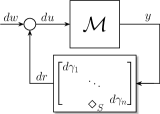
(a) Stratonovich Interpretation

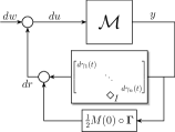
(b) Equivalent Itō Interpretation

Figure 3: (a) A continuous-time causal LTI system $\mathcal{M}$ in feedback with stochastic multiplicative gains $\{d\gamma_{i}\}$ that represent the differential forms of, possibly mutually correlated, Wiener processes. The diamond ”$\diamond_{S}$” in the feedback block indicates a Stratonovich interpretation. (b) The equivalent Itō interpretation, in the mean-square sense, of the block diagram given in (a). The symbol “$\circ$” denotes the Hadamard (element-by-element) product and “$\diamond_{I}$” indicates an Itō interpretation of the multiplicative gains.

The proof of Theorem 1 is given in Section VI. A remark is worth noting here.

Remark IV.1

If $M(0)=0$, the block diagrams in Figures 3 (a) and (b) become identical. This means that there is no difference between Itō and Stratonovich interpretations if the impulse response is zero at initial time. This sort of reintroduces a notion of “strict causality” that forces the Stratonovich interpretation to behave in the same way as that of Itō. Therefore, LTI systems $\mathcal{M}$ with relative degrees $\geq 2$ have the same MSS conditions for both Itō and Stratonovich interpretations.

IV-B Mean-Square Stability Conditions

The MSS setting considered in this paper is given in Figure 2 and is repeated here in Figure 4 to explicitly show the adopted stochastic interpretation of the feedback block. In this section, MSS conditions are given in terms of a linear operator, denoted by $\mathbb{L}$, that acts on a positive semidefinite matrix to produce another positive semidefinite matrix.

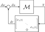
Figure 4: Mean-square stability setting. This figure is similar to the general setting given Figure 2. The only difference is that the stochastic interpretation of the feedback block is encoded by the symbol “$\diamond$” such that $\diamond=\diamond_{I}$ denotes an Itō interpretation, whereas $\diamond=\diamond_{S}$ denotes a Stratonovich interpretation.

Its role is to propagate the steady-state covariance (if it exists) of $du$, denoted by $\bar{\mathbf{U}}$, through the loop to yield that of $dr$, denoted by $\bar{\mathbf{R}}$. This “Loop Gain Operator” (LGO) is the continuous-time counterpart of that defined in [1] for the discrete-time setting. For the Itō setting (i.e. $\diamond=\diamond_{I}$ in Figure 4), the LGO is denoted by $\mathbb{L}_{I}$ and is given by

$$\bar{\mathbf{R}}=\mathbb{L}_{I}\left(\bar{\mathbf{U}}\right) :=\mathbf{\Gamma}\circ\left(\int_{0}^{\infty}M(\tau)\bar{\mathbf{U}}M^{*}(\tau)d\tau\right).$$ (17)

Refer to Section VII for a detailed derivation of the LGO. A key step in the derivation of $\mathbb{L}_{I}$ is showing that $du$ is temporally independent which is required to propagate $\bar{\mathbf{U}}$ in the forward block $\mathcal{M}$ using (12). As will be shown in Section VII-A, this temporal independence is a consequence of (1) the causality of $\mathcal{M}$, (2) the temporal independence of the stochastic multiplicative gains, and (3) the Itō interpretation. However, for the Stratonovich setting (i.e. $\diamond=\diamond_{S}$ in Figure 4), $du$ is not temporally independent. This is a consequence of the nature of the Stratonovich integral in (9) that “looks into the future”. In this case, (12) cannot be used to propagate the covariance in the forward block of Figure 3(a). Nonetheless, one can exploit the block diagram conversion scheme in Section IV-A and rearrange the block diagram in Figure 3(b) so that it looks like the Itō setting as depicted in Figure 5. The equivalent forward block, now denoted by $\mathcal{H}$, is still a causal LTI system whose transfer function is

$$H(s)=\left(I-M(s)G\right)^{-1}M(s),$$ (18)

where $G:=\frac{1}{2}M(0)\circ\mathbf{\Gamma}$ and $M(s)$ is the transfer function of $\mathcal{M}$.

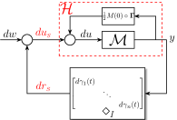
Figure 5: Rearrangement of the block diagram in Figure 3(b)

The input differential signal $du_{S}$ in Figure 5 is now temporally independent and thus (12) can be exploited to propagate the steady state covariance through the equivalent forward block $\mathcal{H}$. Thus, the LGO for the Stratonovich setting propagates the steady-state covariance (if it exists) of $du_{S}$, denoted by $\bar{\mathbf{U}}_{S}$, through the loop of Figure 5 to yield that of $dr_{S}$, denoted by $\bar{\mathbf{R}}_{S}$. It is now denoted by $\mathbb{L}_{S}$ and is given by

$$\bar{\mathbf{R}}_{S}=\mathbb{L}_{S}\left(\bar{\mathbf{U}}_{S}\right) :=\mathbf{\Gamma}\circ\left(\int_{0}^{\infty}H(\tau)\bar{\mathbf{U}}_{S}H^{*}(\tau)d\tau\right),$$ (19)

where $H$ is given in (18). The spectral radius of $\mathbb{L}$ completely characterizes the MSS condition as will be seen next.

Theorem 2

Consider the system in Figure 4 such that Assumptions 1-4 are satisfied. The feedback system is MSS if and only if the two conditions are satisfied

1. The equivalent forward block in Figure 4 has a finite $H^{2}-\text{norm}$.

2. The spectral radius of the loop gain operator is strictly less than 1, i.e. $\rho(\mathbb{L})<1$.

where

• For the Itō interpretation, the equivalent forward block is $\mathcal{M}$, and $\mathbb{L}$ is given in (17).

• For the Stratonovich interpretation, the equivalent forward block is $\mathcal{H}$, whose transfer function is given in (18), $\mathbb{L}$ is given in (19), and Assumption 1 is replaced by Assumption 1^′.

The proof of Theorem 2 is given in Section VII. Observe that, under the Itō interpretations, the covariance matrix $\mathbf{\Gamma}$ only plays a role in the second condition. However, under the Stratonovich interpretation, $\mathbf{\Gamma}$ plays a role in both conditions since the equivalent forward block $\mathcal{H}$ now depends on $\mathbf{\Gamma}$ (Figure 5). Therefore, the conditions of MSS can be very different when different stochastic interpretations are adopted. We close this section by noting that the spectral radius of $\mathbb{L}$ can be numerically calculated using the power iteration explained in [1].

V Application to State Space Realizations & SDEs

In this section, we consider the mean-square stability problems for both the Itō and Stratonovich settings given in Figure 4, but for the special case when $\mathcal{M}$ is given a state space realization. Thus, the underlying equations can be written as SDEs, i.e.

$$dx(t) =Ax(t)dt+Bdu(t);\qquad y(t)=Cx(t)$$

$$du(t) =dw(t)+dr(t)$$

$$dr(t) =d\Gamma(t)\diamond y(t)\quad\text{for}\quad\diamond=\{\diamond_{I},\diamond_{S}\},$$ (20)

where the last equation refers to either an Itō or Stratonovich interpretation. The impulse response of $\mathcal{M}$ can thus be written as $M(t)=Ce^{At}B$. Then, the realization of the loop gain operator, for each interpretation, can be calculated using (17) and (19). Starting with the Itō interpretation, we have

$$\bar{\mathbf{R}} =\mathbb{L}_{I}(\bar{\mathbf{U}}):=\mathbf{\Gamma}\circ\left(\int_{0}^{\infty}M(\tau)\bar{\mathbf{U}}M^{*}(\tau)d\tau\right)$$

$$=\mathbf{\Gamma}\circ\left(C\int_{0}^{\infty}e^{A\tau}B\bar{\mathbf{U}}B^{*}e^{A^{*}\tau}d\tau\right)C$$

$$=\mathbf{\Gamma}\circ\left(C\bar{\mathbf{X}}C\right),$$

where $\bar{\mathbf{X}}:=\int_{0}^{\infty}e^{A\tau}B\bar{\mathbf{U}}B^{*}e^{A^{*}\tau}d\tau$ which satisfies the algebraic Lyapunov equation given by

$$A\bar{\mathbf{X}}+\bar{\mathbf{X}}A^{*}+B\bar{\mathbf{U}}B^{*}=0.$$

For the Stratonovich interpretation, we use Figure 5 to give the equivalent Itō representation. The impulse response of $\mathcal{H}$ in Figure 3(b) can be shown to be $H(t)=Ce^{A_{S}t}$ with $A_{S}=A+1/2B\big{(}(CB)\circ\mathbf{\Gamma}\big{)}C$ and the LGO can be similarly given a realization. To summarize, let $\mathbb{L}_{I}$ and $\mathbb{L}_{S}$ denote the loop gain operators for the Itō and Stratonovich interpretations as given in (17) and (19), respectively. Then their state space realizations are given by

$$\begin{aligned} \bar{\mathbf{R}}&=\mathbb{L}_{k}(\bar{\mathbf{U}})\\ (k&=I,S)\end{aligned} \Leftrightarrow \left\{\begin{aligned} \bar{\mathbf{R}}&=\mathbf{\Gamma}\circ\left(C\bar{\mathbf{X}}C^{*}\right)\\ 0&=A_{k}\bar{\mathbf{X}}+\bar{\mathbf{X}}A_{k}^{*}+B\bar{\mathbf{U}}B^{*};\end{aligned}\right.$$ (21)

where $A_{I}:=A$ and $A_{S}:=A+\frac{1}{2}B\big{(}(CB)\circ\mathbf{\Gamma}\big{)}C$. Therefore, as a direct application of Theorem 2, the necessary and sufficient conditions of MSS are (1) $A_{k}$ is Hurwitz and (2) $\rho(\mathbb{L}_{k})<1$ for $k=I,S$ for Itō and Stratonovich interpretations, respectively.

VI Stochastic Block Diagram Conversion Technique

In this section, we provide a proof for Theorem 1. Consider the Stratonovich setting in Figure 3(a) such that Assumptions 1^′, 2, 3, and 4 are satisfied. The block diagram can be described by a single SIE given in (16) with $\diamond=\diamond_{S}$, and the goal of this section is to show that it is equivalent (in the mean-square sense) to

$$y(t) =\int_{0}^{t}M(t-\tau)dw(\tau)+\int_{0}^{t}M(t-\tau)\diamond_{I}d\Gamma(\tau)y(\tau)$$

$$\qquad\qquad\qquad+\frac{1}{2}\int_{0}^{t}M(t-\tau)\big{(}M_{0}\circ\mathbf{\Gamma}\big{)}y(\tau)d\tau,$$ (22)

where $M(0)$ is denoted by $M_{0}$ for notational convenience. This can be shown by exploiting the following two propositions.

Proposition 1

Consider the SIE given in (VI) (or equivalently (16) with $\diamond=\diamond_{S}$) such that Assumptions 1^′, 2, 3, and 4 are satisfied. Then the second moments of $y$ and its quadratic variation (Section II-12) are both finite over finite intervals. That is, there exist two scalar continuous functions $c_{y}$ and $c_{q}$ such that

$$\sup_{0\leq\tau\leq t}\mathbb{E}\left[\left|\left|y(\tau)\right|\right|^{2}\right]=c_{y}(t);\sup_{0\leq\tau\leq t}\mathbb{E}\left[\langle y\rangle^{2}(\tau)\right]=c_{q}(t).$$ (23)

The proof of the boundedness of $\mathbb{E}\left[\left|\left|y(\tau)\right|\right|^{2}\right]$ is given in [11, Thm 5A] while that of the quadratic variation is given in Section -F. These bounds will be useful to prove Proposition 2.

Proposition 2

Consider the Stratonovich integral

$$S(t):=\int_{0}^{t}M(t-\tau)d\Gamma(\tau)\diamond_{S}y(\tau),$$

where $M$ satisfies Assumption 1, $d\Gamma(t)$ is defined in (13) such that $\boldsymbol{\gamma}$ satisfies Assumption 2, and $y$ is a stochastic process that satisfies (16) with $\diamond=\diamond_{S}$. Then $S(t)=I(t)+\frac{1}{2}R(t)$ in the mean-square sense, where

$$I(t) :=\int_{0}^{t}M(t-\tau)\diamond_{I}d\Gamma(\tau)y(\tau)\qquad\text{and}$$

$$R(t) :=\int_{0}^{t}M(t-\tau)\big{(}M_{0}\circ\mathbf{\Gamma}\big{)}y(\tau)d\tau$$

are Itō and Riemann integrals, respectively.

Proof:

Start by using the definitions of the various integrals in Section II-11 to construct the partial sums over a partition $\mathcal{P}_{N}[0,t]$ (II-9) as

$$S_{N}(t) :=\frac{1}{2}\sum_{k=0}^{N-1}\Big{(}M(t-t_{k+1})\tilde{\Gamma}_{k}y_{k+1}+M(t-t_{k})\tilde{\Gamma}_{k}y_{k}\Big{)}$$ (24)

$$I_{N}(t) :=\sum_{k=0}^{N-1}M(t-t_{k})\tilde{\Gamma}_{k}y_{k}$$

$$R_{N}(t) :=\sum_{k=0}^{N-1}M(t-t_{k})\big{(}M_{0}\circ\mathbf{\Gamma}\big{)}y_{k}\Delta_{k}.$$

The proof is carried out on the partition $\mathcal{P}_{N}[0,t]$ but can be passed to the limit in $L_{2}(p)$ (since it is a Hilbert space and all Cauchy sequences are convergent). More precisely, we are required to prove that $\lim_{N\to\infty}\mathbb{E}\left[D_{N}^{2}(t)\right]=0~{}\forall t\geq 0,$

$$\text{where}\qquad D_{N}(t)=S_{N}(t)-\left(I_{N}(t)+\frac{1}{2}R_{N}(t)\right).$$ (25)

After carrying out a sequence of algebraic manipulations (Appendix -B), the expression of $D_{N}(t)$ can be rewritten as

$$D_{N}(t) =\frac{1}{2}\Big{(}\lambda_{N}(t)+J_{N}(t)+\nu_{N}(t)+\xi_{N}(t)+T^{\zeta}_{N}(t)\Big{)}$$ (26)

$$\qquad+\frac{1}{4}\Big{(}\theta_{N}(t)+\eta_{N}(t)+T^{\alpha}_{N}(t)+T^{\beta}_{N}(t)\Big{)},$$

where

$$\lambda_{N}(t) :=\sum_{k=0}^{N-1}M(t-t_{k})\Big{(}\big{(}\tilde{\boldsymbol{\gamma}}_{k}\tilde{\boldsymbol{\gamma}}_{k}^{*}-\mathbf{\Gamma}\Delta_{k}\big{)}\circ M_{0}\Big{)}y_{k}$$ (27)

$$J_{N}(t) :=\sum_{k=0}^{N-1}\bigg{(}M(t-t_{k+1})-M(t-t_{k})\bigg{)}\tilde{\Gamma}_{k}y_{k}$$

$$\nu_{N}(t) :=\sum_{k=0}^{N-1}\Big{(}M(t-t_{k+1})-M(t-t_{k})\Big{)}\tilde{\Gamma}_{k}M_{0}\tilde{\Gamma}_{k}y_{k}$$

$$\theta_{N}(t) :=\sum_{k=0}^{N-1}M(t-t_{k+1})\tilde{\Gamma}_{k}M_{0}\tilde{\Gamma}_{k}\tilde{y}_{k}$$

$$\eta_{N}(t) :=\sum_{k=0}^{N-1}M(t-t_{k+1})\tilde{\Gamma}_{k}\Big{(}M(\Delta_{k})-M_{0}\Big{)}\tilde{\Gamma}_{k}y_{k}$$

$$\chi_{N}(t) :=\sum_{k=0}^{N-1}M(t-t_{k+1})\tilde{\Gamma}_{k}M(\Delta_{k})\tilde{w}_{k}$$

$$T_{N}^{x}(t) :=\sum_{k=0}^{N-1}M(t-t_{k+1})\tilde{\Gamma}_{k}x_{k}\quad\text{for}\quad x\in\{\alpha,\beta,\zeta\}$$

$$\alpha_{k} :=\sum_{l=0}^{k-1}\bigg{(}M(t_{k+1}-t_{l+1})-M(t_{k}-t_{l+1})\bigg{)}\tilde{\Gamma}_{l}\tilde{y}_{l}$$

$$\beta_{k} :=\sum_{l=0}^{k-1}\bigg{(}M(t_{k+1}-t_{l+1})-M(t_{k}-t_{l+1})$$

$$\qquad\qquad+M(t_{k+1}-t_{l})-M(t_{k}-t_{l})\bigg{)}\tilde{\Gamma}_{l}y_{l}$$

$$\zeta_{k} :=\sum_{l=0}^{k-1}\bigg{(}M(t_{k+1}-t_{l})-M(t_{k}-t_{l})\bigg{)}\tilde{w}_{l}.$$

The rest of the proof shows that the second moment of each term in (26) goes to zero in the limit as $N$ goes to infinity. Note that there is no need to check the expectation of cross terms (Appendix -C).

VI-1 Mean-Square Convergence of $\lambda_{N}(t)$

Recall that $\boldsymbol{\gamma}_{k}$ has independent increments that are also independent from present and past values of $y_{k}$. Furthermore, $\mathbb{E}\left[Z_{k}\right]=0$ with $Z_{k}:=\tilde{\boldsymbol{\gamma}}_{k}\tilde{\boldsymbol{\gamma}}_{k}^{*}-\mathbf{\Gamma}\Delta_{k}$. Then we invoke Lemma -D.6 to yield the following inequality

$$\mathbb{E}\left[\left|\left|\lambda_{N}(t)\right|\right|^{2}\right] \leq\sum_{k=0}^{N-1}\left|\left|M(t-t_{k})\right|\right|^{2}\mathbb{E}\left[\left|\left|\big{(}Z_{k}\circ M_{0}\big{)}\right|\right|^{2}\right]\mathbb{E}\left[\left|\left|y_{k}\right|\right|^{2}\right]$$

$$\leq\left|\left|M_{0}\right|\right|^{2}\sum_{k=0}^{N-1}\left|\left|M(t-t_{k})\right|\right|^{2}\mathbb{E}\left[\left|\left|Z_{k}\right|\right|^{2}\right]\mathbb{E}\left[\left|\left|y_{k}\right|\right|^{2}\right],$$

where the second inequality follows from the sub-multiplicative property of the matrix spectral norm with respect to matrix and Hadamard products (see [14]). Knowing that $\tilde{\boldsymbol{\gamma}}_{k}\sim\mathcal{N}(0,\mathbf{\Gamma}\Delta_{k})$, we can write $\tilde{\boldsymbol{\gamma}}_{k}=\mathbf{\Gamma}^{1/2}\boldsymbol{\xi}_{k}\sqrt{\Delta_{k}}$, where $\mathbf{\Gamma}^{1/2}$ denotes the Cholesky factorization of $\mathbf{\Gamma}$. The random vector $\boldsymbol{\xi}_{k}$ follows a standard multivariate normal distribution for all $k=0,1,...N-1$ such that $\boldsymbol{\xi}_{k}$ and $\boldsymbol{\xi}_{l}$ are independent for $k\neq l$. To bound $\mathbb{E}\left[\left|\left|Z_{k}\right|\right|^{2}\right]$, we proceed as follows

$$\mathbb{E}\left[\left|\left|Z_{k}\right|\right|^{2}\right] =\mathbb{E}\left[\left|\left|\mathbf{\Gamma}^{1/2}(\boldsymbol{\xi}_{k}\boldsymbol{\xi}_{k}^{*}-I)\mathbf{\Gamma}^{1/2}\right|\right|^{2}\Delta_{k}^{2}\right]$$

$$\leq\mathbb{E}\left[\left|\left|\mathbf{\Gamma}\right|\right|\left|\left|\boldsymbol{\xi}_{k}\boldsymbol{\xi}_{k}^{*}-I\right|\right|^{2}\Delta_{k}^{2}\right]$$

$$\leq\mathbb{E}\left[\left|\left|\mathbf{\Gamma}\right|\right|\left|\left|\boldsymbol{\xi}_{k}\boldsymbol{\xi}_{k}^{*}-I\right|\right|^{2}_{F}\Delta_{k}^{2}\right]$$

$$=\mathbb{E}\left[\left|\left|\mathbf{\Gamma}\right|\right|\text{tr}\Big{(}(\boldsymbol{\xi}_{k}\boldsymbol{\xi}_{k}^{*}-I)^{*}(\boldsymbol{\xi}_{k}\boldsymbol{\xi}_{k}^{*}-I)\Big{)}\Delta_{k}^{2}\right]$$

$$=\left|\left|\mathbf{\Gamma}\right|\right|\Delta_{k}^{2}\Big{(}\mathbb{E}\left[\left|\left|\boldsymbol{\xi}_{k}\right|\right|^{4}\right]-2\mathbb{E}\left[\left|\left|\boldsymbol{\xi}_{k}\right|\right|^{2}\right]+n\Big{)}$$

$$=\left|\left|\mathbf{\Gamma}\right|\right|\Delta_{k}^{2}(n^{2}+n).$$

where the second inequality follows from the fact that the Frobenius norm of a matrix is larger than its spectral norm. The last equality follows by using Lemma -D.2, where $n$ is the number of gains $\gamma_{i}$. Finally, we obtain

$$\mathbb{E}\left[\left|\left|\lambda_{N}(t)\right|\right|^{2}\right] \leq\left|\left|M_{0}\right|\right|^{2}c_{M}^{2}(t)\left|\left|\mathbf{\Gamma}\right|\right|(n^{2}+n)c_{y}(t)\sum_{k=0}^{N-1}\Delta_{k}^{2}\underset{N\to\infty}{\longrightarrow}0,$$

where Assumption 1 and (23) are exploited.

VI-2 Mean-Square Convergence of $J_{N}(t)$

This partial sum is similar to that of $\lambda_{N}(t)$, and thus we define $F_{k}(t):=M(t-t_{k+1})-M(t-t_{k})$ and invoke Lemma -D.6 again to yield

$$\mathbb{E}\left[\left|\left|J_{N}(t)\right|\right|^{2}\right] \leq\sum_{k=0}^{N-1}\left|\left|F_{k}(t)\right|\right|^{2}\mathbb{E}\left[\left|\left|\tilde{\Gamma}_{k}\right|\right|^{2}\right]\mathbb{E}\left[\left|\left|y_{k}\right|\right|^{2}\right]$$

$$\leq c_{y}(t)\text{tr}\left(\mathbf{\Gamma}\right)\sum_{k=0}^{N-1}\left|\left|M(t-t_{k+1})-M(t-t_{k})\right|\right|^{2}\Delta_{k}$$

$$\leq c_{y}(t)\text{tr}\left(\mathbf{\Gamma}\right)\mathbf{\Delta}\mathcal{Q}\mathcal{V}_{0}^{t}\left(M\right)\underset{N\to\infty}{\longrightarrow}0,$$

where the second inequality follows from (23), Lemma -D.2 and the fact that $\left|\left|\tilde{\Gamma}_{k}\right|\right|\leq\left|\left|\tilde{\boldsymbol{\gamma}}_{k}\right|\right|$ since $\tilde{\Gamma}_{k}=\mathcal{D}(\tilde{\boldsymbol{\gamma}}_{k})$ so that

$$\mathbb{E}\left[\left|\left|\tilde{\Gamma}_{k}\right|\right|^{2}\right]\leq\text{tr}\left(\mathbf{\Gamma}\right)\Delta_{k}.$$ (28)

The last inequality follows from the fact that the quadratic variation of $M$ is finite (Lemma -E.1).

VI-3 Mean-Square Convergence of $\nu_{N}(t)$

By using the same previous definition of $F_{k}(t)$, invoke Lemma -D.5 (with $X_{k}:=\tilde{\Gamma}_{k}M_{0}\tilde{\Gamma}_{k}$) to yield

$$\mathbb{E}\left[\left|\left|\nu_{N}(t)\right|\right|^{2}\right]$$

$$\leq\left(\sum_{k=0}^{N-1}\left|\left|F_{k}(t)\right|\right|\left(\mathbb{E}\left[\left|\left|\tilde{\Gamma}_{k}M_{0}\tilde{\Gamma}_{k}\right|\right|^{2}\right]\mathbb{E}\left[\left|\left|y_{k}\right|\right|^{2}\right]\right)^{\frac{1}{2}}\right)^{2}$$

$$\leq c_{y}(t)\left|\left|M_{0}\right|\right|^{2}\left(\sum_{k=0}^{N-1}\left|\left|F_{k}(t)\right|\right|\left(\mathbb{E}\left[\left|\left|\tilde{\Gamma}_{k}\right|\right|^{4}\right]\right)^{\frac{1}{2}}\right)^{2}$$

$$\leq c_{y}(t)\left|\left|M_{0}\right|\right|^{2}c(2,n)\mathbf{\Delta}\Big{(}\mathcal{T}\mathcal{V}_{0}^{t}\left(M\right)\Big{)}^{2}\underset{N\to\infty}{\longrightarrow}0,$$

where the second inequality follows from (23) and the sub-multiplicative property of the spectral norm. The third inequality follows from Lemma -D.2 where

$$\mathbb{E}\left[\left|\left|\tilde{\Gamma}_{k}\right|\right|^{4}\right]\leq c(2,n)\left|\left|\mathbf{\Gamma}\right|\right|^{2}\Delta_{k}^{2},$$ (29)

and the last inequality follows from the fact that the total variation of $M$ is finite (Lemma -E.1).

VI-4 Mean-Square Convergence of $\eta_{N}(t)$

In a similar fashion to the previous calculation, define $G_{k}:=M(\Delta_{k})-M_{0}$ and invoke Lemma -D.5 (with $X_{k}:=\tilde{\Gamma}_{k}G_{k}\tilde{\Gamma}_{k}$) to yield

$$\mathbb{E}\left[\left|\left|\eta_{N}(t)\right|\right|^{2}\right] \leq\left(\sum_{k=0}^{N-1}\left|\left|M(t-t_{k})\right|\right|\left(\mathbb{E}\left[\left|\left|\tilde{\Gamma}_{k}G_{k}\tilde{\Gamma}_{k}\right|\right|^{2}\right]\mathbb{E}\left[\left|\left|y_{k}\right|\right|^{2}\right]\right)^{\frac{1}{2}}\right)^{2}$$

$$\leq c_{y}(t)c_{M}^{2}(t)\left(\sum_{k=0}^{N-1}\left|\left|M(\Delta_{k})-M_{0}\right|\right|\left(\mathbb{E}\left[\left|\left|\tilde{\Gamma}_{k}\right|\right|^{4}\right]\right)^{\frac{1}{2}}\right)^{2}$$

$$\leq c_{y}(t)c_{M}^{2}(t)c(4,n)\left|\left|\mathbf{\Gamma}\right|\right|^{2}\left(\sum_{k=0}^{N-1}\left|\left|M(\Delta_{k})-M_{0}\right|\right|\Delta_{k}\right)^{2}$$

$$\underset{N\to\infty}{\longrightarrow}0,$$

where the second inequality follows from (23), Assumption 1, and the sub-multiplicative property of the spectral norm. Again, the last inequality follows from (29). The limit is zero because Assumption 1 guarantees that $M$ is right-continuous at $t=0$.

VI-5 Mean-Square Convergence of $\chi_{N}(t)$

Since $w$ and $\{\gamma_{i}\}$ are uncorrelated (Assumption 4), invoking Lemma -D.6 yields

$$\mathbb{E}\left[\left|\left|\chi_{N}(t)\right|\right|^{2}\right] \leq\sum_{k=0}^{N-1}\left|\left|M(t-t_{k+1})\right|\right|^{2}\mathbb{E}\left[\left|\left|\tilde{\Gamma}_{k}\right|\right|^{2}\right]\mathbb{E}\left[\left|\left|M(\Delta_{k})\tilde{w}_{k}\right|\right|^{2}\right]$$

$$\leq c_{M}^{4}(t)\text{tr}\left(\mathbf{\Gamma}\right)\sum_{k=0}^{N-1}\Delta_{k}\text{tr}\left(\mathbf{W}_{k}\right)\Delta_{k}$$

$$\leq c_{M}^{4}(t)\text{tr}\left(\mathbf{\Gamma}\right)c_{w}(t)\sum_{k=0}^{N-1}\Delta_{k}^{2}\underset{N\to\infty}{\longrightarrow}0,$$

where the second inequality follows from Assumptions 1 and 3 and (28). The last inequality follows because under Assumption 3, $\exists$ a continuous scalar function $c_{w}$ such that

$$\sup_{0\leq\tau\leq t}\text{tr}\left(\mathbf{W}(\tau)\right)=c_{w}(t).$$ (30)

VI-6 Mean-Square Convergence of $\theta_{N}(t)$

By invoking Lemma -D.4, we obtain the following inequality

$$\mathbb{E}\left[\left|\left|\theta_{N}(t)\right|\right|^{2}\right] \leq\sum_{k=0}^{N-1}\left|\left|M(t-t_{k+1})\right|\right|^{2}\left(\mathbb{E}\left[\left|\left|\tilde{\Gamma}_{k}M_{0}\tilde{\Gamma}_{k}\right|\right|^{4}\right]\right)^{\frac{1}{2}}$$

$$\qquad\qquad\times\left(\mathbb{E}\left[\left(\sum_{k=0}^{N-1}\left|\left|\tilde{y}_{k}\right|\right|^{2}\right)^{2}\right]\right)^{\frac{1}{2}},$$

where the second term converges to $\left(\mathbb{E}\left[\langle y\rangle^{2}(t)\right]\right)^{\frac{1}{2}}\leq\sqrt{c_{q}(t)}$ defined in (23). Now apply the submultiplicative property of the spectral norm to yield

$$\mathbb{E}\left[\left|\left|\theta_{N}(t)\right|\right|^{2}\right]\leq\sqrt{c_{q}(t)}\left|\left|M_{0}\right|\right|^{2}\sum_{k=0}^{N-1}\left|\left|M(t-t_{k+1})\right|\right|^{2}\left(\mathbb{E}\left[\left|\left|\tilde{\Gamma}_{k}\right|\right|^{8}\right]\right)^{\frac{1}{2}}$$

$$\leq\sqrt{c_{q}(t)}\sqrt{c(4,n)}\left|\left|\mathbf{\Gamma}\right|\right|^{2}c_{M}^{2}(t)\left|\left|M_{0}\right|\right|^{2}\sum_{k=0}^{N-1}\Delta_{k}^{2}\underset{N\to\infty}{\longrightarrow}0,$$

where the last inequality follows from Assumption 1 and Lemma -D.2 where $c(4,n)\left|\left|\mathbf{\Gamma}\right|\right|^{4}\Delta_{k}^{4}$ serves as an upper bound for the eighth moment $\mathbb{E}\left[\left|\left|\tilde{\Gamma}_{k}\right|\right|^{8}\right]$.

VI-7 Mean-Square Convergence of $T_{N}^{\alpha}(t),T_{N}^{\beta}(t)$ and $T_{N}^{\zeta}(t)$

Observe using (27) that the pairs $(\tilde{\Gamma}_{k},\alpha_{k}),(\tilde{\Gamma}_{k},\beta_{k})$ and $(\tilde{\Gamma}_{k},\zeta_{k})$ are independent for all $k=0,1,\cdots,N-1$. Then, for $x\in\{\alpha,\beta,\zeta\}$, invoking Lemma -D.6 yields

$$\mathbb{E}\left[\left|\left|T_{N}^{x}(t)\right|\right|^{2}\right] \leq\sum_{k=0}^{N-1}\left|\left|M(t-t_{k+1})\right|\right|^{2}\mathbb{E}\left[\left|\left|\tilde{\Gamma}_{k}\right|\right|^{2}\right]\mathbb{E}\left[\left|\left|x_{k}\right|\right|^{2}\right]$$

$$\leq c_{M}^{2}(t)\text{tr}\left(\mathbf{\Gamma}\right)\sum_{k=0}^{N-1}\mathbb{E}\left[\left|\left|x_{k}\right|\right|^{2}\right]\Delta_{k},$$

where the last inequality follows from Assumption 1 and (28). Now, we examine $\mathbb{E}\left[\left|\left|\alpha_{k}\right|\right|^{2}\right]$. Define $F_{k,l}:=M(t_{k+1}-t_{l+1})-M(t_{k}-t_{l+1})$ and invoke Lemma -D.4 to yield

$$\mathbb{E}\left[\left|\left|\alpha_{k}\right|\right|^{2}\right] \leq\sum_{l=0}^{k-1}\left|\left|F_{k,l}\right|\right|^{2}\left(\mathbb{E}\left[\left|\left|\tilde{\Gamma}_{l}\right|\right|^{4}\right]\right)^{\frac{1}{2}}\left(\mathbb{E}\left[\sum_{l=0}^{k-1}\left|\left|\tilde{y}_{l}\right|\right|^{2}\right]\right)^{\frac{1}{2}}$$

$$\leq\sqrt{c(2,n)}\left|\left|\mathbf{\Gamma}\right|\right|\sqrt{c_{q}(t)}\sum_{l=0}^{k-1}\left|\left|F_{k,l}\right|\right|^{2}\Delta_{l}$$

$$\leq\sqrt{c(2,n)}\left|\left|\mathbf{\Gamma}\right|\right|\sqrt{c_{q}(t)}\mathbf{\Delta}\mathcal{Q}\mathcal{V}_{0}^{t}\left(M\right),$$

where $\mathbf{\Delta}=\sup_{l}\Delta_{l}$. Note that the second inequality follows from (23) and (29), and the third inequality follows by observing that the sum converges to the quadratic variation of $M$ on the interval $[0,t_{k}]$ (Appendix -E). The last equality exploits the fact that $\mathcal{Q}\mathcal{V}_{0}^{t}\left(M\right)$ is an increasing function in $t$. Substituting in $\mathbb{E}\left[\left|\left|T_{N}^{\alpha}(t)\right|\right|^{2}\right]$ yields

$$\mathbb{E}\left[\left|\left|T_{N}^{\alpha}(t)\right|\right|^{2}\right] \leq c_{M}^{2}(t)\text{tr}\left(\mathbf{\Gamma}\right)\sqrt{c(2,n)}\left|\left|\mathbf{\Gamma}\right|\right|\sqrt{c_{q}(t)}\mathbf{\Delta}\mathcal{Q}\mathcal{V}_{0}^{t}\left(M\right)\sum_{k=0}^{N-1}\Delta_{k}$$

$$\leq c_{M}^{2}(t)\text{tr}\left(\mathbf{\Gamma}\right)\sqrt{c(2,n)}\left|\left|\mathbf{\Gamma}\right|\right|\sqrt{c_{q}(t)}\mathbf{\Delta}\mathcal{Q}\mathcal{V}_{0}^{t}\left(M\right)t\underset{N\to\infty}{\longrightarrow}0.$$

Recalling from Appendix -C that there is no need to check the convergence of the cross terms, the same arguments used for $\mathbb{E}\left[\left|\left|T_{N}^{\alpha}(t)\right|\right|^{2}\right]$ can be used here to show that

$$\mathbb{E}\left[\left|\left|T_{N}^{\beta}(t)\right|\right|^{2}\right]\underset{N\to\infty}{\longrightarrow}0\qquad\text{and}\qquad\mathbb{E}\left[\left|\left|T_{N}^{\zeta}(t)\right|\right|^{2}\right]\underset{N\to\infty}{\longrightarrow}0.$$

This completes the proof of Proposition 2. ∎ A direct application of Proposition 2 to (16) with $\diamond=\diamond_{S}$ yields (VI). This is exactly the result shown in Figure 3(b) and given in Theorem 1.

VII Loop Gain Operator & MSS Conditions

In this section, we give the mathematical derivations of the LGO (17) for the Itō setting. The same analysis can be carried out for the Stratonovich case by using the conversion scheme developed in Section IV-A. We first lay down the necessary framework to construct a deterministic block diagram that describes the continuous-time evolution of the covariance matrices of the various signals in the loop (see Figure 7). Once this deterministic setting is constructed, the MSS analysis from there onwards resembles that of the discrete-time counterpart in [1].

VII-A Stochastic Block Diagram Interpretation

Consider the stochastic continuous-time setting depicted in Figure 6(a) satisfying Assumptions 1-4. It is the same as the general setting in Figure 2, but it also indicates an Itō interpretation of the stochastic multiplicative gains. By using the definition of Itō integrals in Section II-11, we construct a discrete-time block diagram, depicted in Figure 6(b), which explicitly describes the Itō interpretation of Figure 6(a). In fact, it is constructed by using a partition $\mathcal{P}_{N}[0,t]$ of $N$ subintervals on $[t_{0},t_{N}]:=[0,t]$ as described in Section II-11. Therefore, Figure 6(a) can be interpreted as the limit of Figure 6(b) as $N\to\infty$. Note that $\mathcal{M}_{N}$ denotes a finite dimensional approximation of $\mathcal{M}$ on the partition $\mathcal{P}_{N}[0,t]$, i.e.

$$y=\mathcal{M}_{N}\tilde{u}\Longleftrightarrow y_{N}=\sum_{k=0}^{N-1}M(t_{N}-t_{k})\tilde{u}_{k},$$

where the “tilde” is used to denote the increments of a signal (refer to Section II-11).

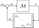
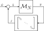
(a) Continuous-Time Setting	(b) Discrete-Time Setting

Figure 6: A causal LTI system $\mathcal{M}$ in feedback with stochastic multiplicative gains $\{d\gamma_{i}\}$ that represent the differential forms of, possibly mutually correlated, Wiener processes. Figure (a) shows the continuous-time MSS setting when the Itō interpretation is adopted. Figure (b) explicitly describes the Itō interpretation of Figure (a) by using a partition $\mathcal{P}_{N}[0,t]$ of $N$ subintervals as explained in II-11. In fact, Figure (a) is interpreted as the limit of Figure (b) as $N\to\infty$.

The equations describing the block diagrams in Figures 6(a) and (b) can be respectively written as

The rest of this subsection shows that by adopting the Itō interpretation (31b), the stochastic signal $r$ will have independent increments. Furthermore, we will derive the expression that describes the propagation of the instantaneous covariance through the feedback block. The analysis is carried out using Figure 6(b) and then is passed to the limit as $N\to\infty$.

VII-A1 Disturbance-to-signals mapping

It is fairly straightforward to show that the disturbance $\tilde{w}$ is mapped to the various signals in the loop as

$$\begin{bmatrix}\tilde{u}\\ y\\ \tilde{r}\end{bmatrix}=\begin{bmatrix}(I-\tilde{\Gamma}\mathcal{M}_{N})^{-1}\\ (I-\mathcal{M}_{N}\tilde{\Gamma})^{-1}\mathcal{M}_{N}\\ (I-\tilde{\Gamma}\mathcal{M}_{N})^{-1}\tilde{\Gamma}\mathcal{M}_{N}\end{bmatrix}\tilde{w}.$$ (32)

VII-A2 Independence of $\big{(}d\Gamma(t),y(\tau)\big{)}$ for $\tau\leq t$

This can be shown by analyzing the second equation in (32). Examining the operator $(I-\mathcal{M}_{N}\tilde{\Gamma})^{-1}$ allows us to write it, over the time horizon of the partition $\mathcal{P}_{N}[0,t]$, as

$$\begin{bmatrix}I&&&\\ -M(t_{1}-t_{0})\tilde{\Gamma}_{0}&I&&\\ &\ddots&\ddots&\\ -M(t_{N}-t_{0})\tilde{\Gamma}_{0}&\cdots&-M(t_{N}-t_{N-1})\tilde{\Gamma}_{N-1}&I\end{bmatrix}^{-1}=\begin{bmatrix}I&&\\ &\ddots&\\ *&&I\end{bmatrix},$$

where $*$ denotes the blocks of matrices that are functions of $\tilde{\Gamma}_{k}$ for $k=0,1,...,N-1$. Hence the second equation in (32) can be written as

$$\begin{bmatrix}y_{0}\\ \vdots\\ y_{N}\end{bmatrix}~{}=\begin{bmatrix}I&&\\ &\ddots&\\ *&&I\end{bmatrix}\begin{bmatrix}I&&&\\ M(t_{1}-t_{0})&I&&\\ &\ddots&\ddots&\\ M(t_{N}-t_{0})&\cdots&M(t_{N}-t_{N-1})&I\end{bmatrix}\begin{bmatrix}\tilde{w}_{0}\\ \vdots\\ \tilde{w}_{N}\end{bmatrix}.$$

Clearly, $y_{N}$ does not depend on $\tilde{\Gamma}_{N}$ for any positive integer $N$. Furthermore, by carrying out a similar reasoning, it is straightforward to see that $\tilde{\Gamma}_{N}$ is independent of the past values of all the signals in the loop (particularly $y$). This analysis shows that $(\tilde{\Gamma}_{N},y_{k})$ are independent for $k\leq N$. Finally, taking the limit as $N\to\infty$ completes the argument.

VII-A3 Temporal independence of the increments of $r$

The following calculation shows that $r$ has independent increments. For $k<l$, we have

$$\mathbb{E}\left[\tilde{r}_{k}\tilde{r}^{*}_{l}\right] =\mathbb{E}\left[\tilde{\Gamma}_{k}y_{k}y_{l}^{*}\tilde{\Gamma}^{*}_{l}\right]=\mathbb{E}\left[\tilde{\Gamma}_{k}y_{k}y_{l}^{*}\right]\mathbb{E}\left[\tilde{\Gamma}^{*}_{l}\right]=0,$$

where the third equality holds because $\tilde{\Gamma}$ has a zero-mean, and the second equality follows because $\Gamma$ has independent increments (Wiener process) and also $\tilde{\Gamma}$ is independent of present and past values of $y$ (Section VII-A2).

The combination between the causality of $\mathcal{M}$ and the Itō interpretation introduces a sort of “strict causality” in continuous-time systems. Thus the multiplicative, temporally independent gains $\{d\gamma_{i}(t)\}$ has a “whitening” effect. In fact, although $y$ has nonzero temporal correlations, the signal $r$ is guaranteed to have independent increments $dr$, i.e. $\mathbb{E}\left[dr(t)dr^{*}(\tau)\right]=0,~{}\forall t\neq\tau$.

Finally, the instantaneous covariance of $dr$ is calculated as

$$\mathbb{E}\left[dr(t)dr(t)^{*}\right] =\mathbb{E}\left[d\Gamma(t)y(t)y^{*}(t)d\Gamma^{*}(t)\right]$$

$$=\mathbb{E}\bigg{[}d\Gamma(t)\mathbb{E}\left[y(t)y^{*}(t)\right]d\Gamma^{*}(t)\bigg{]}$$

$$=\mathbf{\Gamma}\circ\mathbf{Y}(t)dt=:\mathbf{R}(t)dt,$$

where the second equality is a consequence of Lemma -D.1 since $d\Gamma(t)$ and $y(t)$ are independent (Section VII-A2). The third equality is an immediate consequence of the fact that $d\Gamma(t)=\mathcal{D}\big{(}d\boldsymbol{\gamma}(t)\big{)}$. Finally, we have

$$\mathbf{R}(t)=\mathbf{\Gamma}\circ\mathbf{Y}(t).$$ (33)

VII-B Covariance Feedback System

The goal of this section is to construct a deterministic feedback system that describes the evolution of the instantaneous covariance matrices of the various signals in Figure 6 and finally derive the expression of the LGO given in (17).

In the previous section, we showed that $r$ has temporally independent increments. As a result, it is straightforward to see that $u$ also has temporally independent increments, because for $k<l$ we have

$$\mathbb{E}\left[\tilde{u}_{k}\tilde{u}_{l}^{*}\right] =\mathbb{E}\left[(\tilde{w}_{k}+\tilde{r}_{k})(\tilde{w}_{l}+\tilde{r}_{l})^{*}\right]$$

$$=\mathbb{E}\left[\tilde{w}_{k}\tilde{w}_{l}^{*}\right]+\mathbb{E}\left[\tilde{r}_{k}\tilde{r}_{l}^{*}\right]+\mathbb{E}\left[\tilde{r}_{k}\tilde{w}_{l}\right]+\mathbb{E}\left[\tilde{w}_{k}\tilde{r}_{l}^{*}\right]$$

$$=0+0+0+\mathbb{E}\left[\tilde{w}_{k}y_{l}^{*}\tilde{\Gamma}_{l}^{*}\right]$$

$$=\mathbb{E}\left[\tilde{w}_{k}y_{l}^{*}\right]\mathbb{E}\left[\tilde{\Gamma}_{l}^{*}\right]=0,$$

where the third equality follows from the fact that $w$ (Wiener process) and $r$ (Section VII-A3) both have independent increments and the fact that $w$ is independent of past values of all the signals in the loop. The fourth equality follows from Section VII-A2 and the assumption that $w$ and $\Gamma$ are independent. Finally, passing to the limit as $N\to\infty$ yields that $du$ is temporally independent.

As for the instantaneous covariance of $\tilde{u}$, we have

$$\mathbb{E}\left[\tilde{u}_{k}\tilde{u}_{k}^{*}\right] =\mathbb{E}\left[\tilde{w}_{k}\tilde{w}_{k}^{*}\right]+\mathbb{E}\left[\tilde{r}_{k}\tilde{r}_{k}^{*}\right]+\mathbb{E}\left[\tilde{r}_{k}\tilde{w}_{k}^{*}\right]+\mathbb{E}\left[\tilde{w}_{k}\tilde{r}_{k}^{*}\right]$$

$$=\mathbf{W}_{k}\Delta_{k}+\mathbf{R}_{k}\Delta_{k}+\mathbb{E}\left[\tilde{\Gamma}_{k}y_{k}\tilde{w}_{k}^{*}\right]+\mathbb{E}\left[\tilde{w}_{k}y_{k}^{*}\tilde{\Gamma}_{k}^{*}\right]$$

$$=(\mathbf{W}_{k}+\mathbf{R}_{k})\Delta_{k}+0+0=:\mathbf{U}_{k}\Delta_{k}.$$

Therefore, the addition junction in Figure 6 remains as an addition operation on the associated covariance matrices, i.e.

$$\mathbf{U}(t)=\mathbf{W}(t)+\mathbf{R}(t).$$ (34)

Furthermore, the propagation of the covariance through the forward block of Figure 6 is given by (11) which requires the input $du$ to be temporally independent for its validity. Finally, the propagation of the covariance through the feedback block is given by (33). Therefore, (11), (33) and (34) can be used to construct the deterministic feedback block diagram depicted in Figure 7, where each signal is matrix-valued.

Figure 7: A deterministic block diagram describing the evolution of the covariance matrices of the various signals in the feedback loop of Figure 6(a). The forward block represents a convolution integral of matrices and the feedback block represents a Hadamard (element-by-element) product. Note that all the covariance matrices in the loop are positive semi-definite and non-decreasing in time when $\mathbf{W}$ is non-decreasing, i.e. for $t_{2}\geq t_{1}$, $\mathbf{W}(t_{2})-\mathbf{W}(t_{1})\geq 0$ (refer to [1]).

The advantage of the covariance feedback system in Figure 7 is that it describes a deterministic dynamical system unlike its corresponding stochastic feedback system in Figure 6. Before we construct the loop gain operator, we give a remark.

Remark VII.1

All the covariance signals in Figure 7 are monotone. Particularly, if $t_{1}\leq t_{2}$ then $\mathbf{U}(t_{1})\leq\mathbf{U}(t_{2})$, where the matrix ordering is taken in the usual positive semidefinite sense. Refer to [1, Section II-E].

VII-C Loop Gain Operator

We are now equipped with all the necessary tools to define the continuous-time counterpart of the LGO introduced in [1]. Over a finite time horizon $[0,t]$, the instantaneous covariance $\mathbf{R}(t)$ can be expressed in terms of $\{\mathbf{U}(\tau),0\leq\tau\leq t\}$ using (11) and (33) as

$$\mathbf{R}(t) =\mathbf{\Gamma}\circ\mathbf{Y}(t)$$

$$=\mathbf{\Gamma}\circ\left(\int_{0}^{t}M(t-s)\mathbf{U}(s)M(t-s)ds\right)$$

$$\mathbf{R}(t) =\mathbf{\Gamma}\circ\left(\int_{0}^{t}M(\tau)\mathbf{U}(t-\tau)M^{*}(\tau)d\tau\right).$$ (35)

The previous calculation motivates the definition of a finite dimensional linear operator over the infinite time horizon, i.e. as $t\to\infty$

$$\bar{\mathbf{R}}=\mathbb{L}\left(\bar{\mathbf{U}}\right) :=\mathbf{\Gamma}\circ\left(\int_{0}^{\infty}M(\tau)\bar{\mathbf{U}}M^{*}(\tau)d\tau\right)$$ (36)

where $\bar{\mathbf{U}}$ and $\bar{\mathbf{R}}$ are the steady-state limits (if they exist) of the covariances. This linear operator acts on a matrix to produce another matrix, and it propagates the steady state covariance $\bar{\mathbf{U}}$ “once around the loop” to produce the steady state covariance $\bar{\mathbf{R}}$ (and thus the name loop gain operator, refer to Figure 7). Before moving to the next section, we define here a truncated version of the LGO as

$$\mathbb{L}_{T}\left(X\right):=\mathbf{\Gamma}\circ\left(\int_{0}^{T}M(\tau)XM^{*}(\tau)d\tau\right),$$ (37)

which will be useful when proving Theorem 2. Before stating the proof, we summarize some useful properties of the LGO in three remarks.

Remark VII.2

The operator $\mathbb{L}_{T}$ defined in (37) is a monotone operator, i.e. if $0\leq X\leq Y$, then $0\leq\mathbb{L}_{T}(X)\leq\mathbb{L}_{T}(Y)$. The same property holds for $\mathbb{L}$ defined in $(\ref{Eqn: ITH LGO})$ since $\mathbb{L}=\lim_{T\to\infty}\mathbb{L}_{T}$. Refer to [1, Section II-E] for details, noting that the same arguments also hold for integrals as well as summations.

Remark VII.3

The operator $\mathbb{L}_{T}$ is also monotone in time, i.e. if $T_{1}\leq T_{2}$, then $0\leq\mathbb{L}_{T_{1}}(X)\leq\mathbb{L}_{T_{2}}(X)$ for any $X\geq 0$. This is easy to validate by checking that $\mathbb{L}_{T_{2}}(X)-\mathbb{L}_{T_{1}}(X)$ is positive semidefinite. Consequently, for any $T>0$ and $X\geq 0$, we have $0\leq\mathbb{L}_{T}(X)\leq\mathbb{L}(X)$.

Remark VII.4

The spectral radius of $\mathbb{L}$ is its largest eigenvalue which is guaranteed to be a real number. Furthermore, the “eigen-matrix” associated with the largest eigenvalue is guaranteed to be positive semidefinite. That is, if $\rho(\mathbb{L})$ denotes the spectral radius of $\mathbb{L}$, then $\exists\hat{\mathbf{U}}\geq 0$ s.t. $\mathbb{L}(\hat{\mathbf{U}})=\rho(\mathbb{L})\hat{\mathbf{U}}$. Note that $\hat{\mathbf{U}}$ is the matrix counterpart of the Perron-Frobenius vector for matrices with nonnegative entries. This is the covariance mode that has the fastest growth rate if MSS is violated, and therefore we refer to $\hat{\mathbf{U}}$ as the worst-case covariance. (Refer to [1, Thm 2.3] for more details.)

VII-D MSS Conditions

Equipped with the LGO, we can now present the proof of Theorem 2. The proof is very similar to the discrete-time counterpart in [1], and thus some of the details are omitted.

Proof:

VII-D1 if

Using (34) and (VII-C), $\mathbf{U}(t)$ can be written as

$$\mathbf{U}(t) =\mathbf{\Gamma}\circ\left(\int_{0}^{t}M(\tau)\mathbf{U}(t-\tau)M^{*}(\tau)d\tau\right)+\mathbf{W}(t)$$

$$\leq\mathbf{\Gamma}\circ\left(\int_{0}^{t}M(\tau)\mathbf{U}(t)M^{*}(\tau)d\tau\right)+\mathbf{W}(t)$$

$$\leq\mathbb{L}\Big{(}\mathbf{U}(t)\Big{)}+\mathbf{W}(t),$$

where the first inequality follows from Schur’s theorem [15, Thm 2.1] and the fact that $\mathbf{U}(t-\tau)\leq\mathbf{U}(t)$ for all $\tau\in[0,t]$ (Remark VII.1). The second inequality follows from Remark VII.3. To obtain an upper bound on $\mathbf{U}(t)$, we let $\mathbb{I}$ denote the identity operator and rearrange to obtain

$$(\mathbb{I}-\mathbb{L})\mathbf{U}(t) \leq\mathbf{W}(t)\leq\bar{\mathbf{W}}$$

$$\mathbf{U}(t) \leq(\mathbb{I}-\mathbb{L})^{-1}\bar{\mathbf{W}},$$

where the second equality is obtained by replacing $\mathbf{W}(t)$ with its steady state value $\bar{\mathbf{W}}$ since it is assumed to be monotone (Assumption 3). The third inequality is obtained by applying [1, Thm 2.3] which guarantees that the operator $(\mathbb{I}-\mathbb{L})^{-1}$ exists and is monotone whenever $\mathbb{L}$ is monotone and $\rho(\mathbb{L})<1$. Finally the stability of $\mathcal{M}$ (finite $H^{2}-\text{norm}$) guarantees that all other covariance signals in the loop of Figure 7 are also uniformly bounded thus guaranteeing MSS.

VII-D2 only if

First it is straightforward to show that MSS is lost if the $H^{2}$-norm of $M$ is infinite (regardless of the value of $\rho(\mathbb{L}))$. Using Figure 7, we can write the covariance $\mathbf{Y}(t)$ as

$$\mathbf{Y}(t) =\int_{0}^{t}M(t-\tau)\mathbf{U}(\tau)M^{*}(t-\tau)d\tau$$

$$=\int_{0}^{t}M(t-\tau)\Big{(}\mathbf{W}(\tau)+\mathbf{\Gamma}\circ\mathbf{Y}(\tau)\Big{)}M^{*}(t-\tau)d\tau$$

$$\geq\int_{0}^{t}M(t-\tau)\mathbf{W}(\tau)M^{*}(t-\tau)d\tau,$$

where the inequality follows from the fact that $\mathbf{\Gamma}\circ\mathbf{Y}(\tau)$ is positive semidefinite. Thus, clearly $\mathbf{Y}(t)$ grows unboundedly when $M$ has an infinite $H^{2}$-norm (take $\mathbf{W}(t)=I$ for example).

Next, assume that $M$ has a finite $H^{2}$-norm. We will show that if $\rho(\mathbb{L})\geq 1$, then $\mathbf{U}(t)$ grows unboundedly in time. We do so by examining $\mathbf{U}(t)$ at the time samples $t_{k}:=kT$, where $k$ is a positive integer and $T>0$. Using Figure 7, we obtain

$$\mathbf{U}(t_{k}) =\mathbf{\Gamma}\circ\int_{0}^{t_{k}}M(t_{k}-\tau)\mathbf{U}(\tau)M^{*}(t_{k}-\tau)d\tau+\mathbf{W}(t_{k})$$

$$\geq\mathbf{\Gamma}\circ\int_{t_{k-1}}^{t_{k}}M(t_{k}-\tau)\mathbf{U}(\tau)M^{*}(t_{k}-\tau)d\tau+\mathbf{W}(t_{k})$$

$$\geq\mathbf{\Gamma}\circ\int_{t_{k-1}}^{t_{k}}M(t_{k}-\tau)\mathbf{U}(t_{k-1})M^{*}(t_{k}-\tau)d\tau+\mathbf{W}(t_{k})$$

$$\geq\mathbf{\Gamma}\circ\int_{0}^{T}M(s)\mathbf{U}(t_{k-1})M^{*}(s)ds+\mathbf{W}(t_{k})$$

$$=\mathbb{L}_{T}\Big{(}\mathbf{U}(t_{k-1})\Big{)}+\mathbf{W}(t_{k})$$

$$\mathbf{U}(t_{k}) \geq\mathbb{L}_{T}^{k}\Big{(}\mathbf{U}(0)\Big{)}+\sum_{r=0}^{k-1}\mathbb{L}_{T}^{r}\Big{(}\mathbf{W}(t_{k-r})\Big{)},$$ (38)

where the first inequality follows from the fact that the integrand is positive semidefinite, the second inequality follows because $\mathbf{U}(\tau)\geq\mathbf{U}(t_{k-1})$ for $\tau\in[t_{k-1},t_{k}]$, and the third inequality is a consequence of applying the change of variable $s:=t_{k}-\tau$. The last inequality is a consequence of a simple induction argument that exploits the monotonicity of $\mathbb{L}_{T}$ (Remark VII.2). Establishing the inequality (VII-D2) allows us to use the same arguments in [1] (repeated here for completeness) to show that $\mathbf{U}(t_{k})$ grows unboundedly.

Set the exogenous covariance $\mathbf{W}(t_{k})=\hat{\mathbf{U}}$, where $\hat{\mathbf{U}}$ is the worst-case covariance described in Remark VII.4. Note that the initial covariance is $\mathbf{U}_{0}=\hat{\mathbf{U}}$. Substituting in (VII-D2) yields

$$\mathbf{U}(t_{k})\geq\sum_{r=0}^{k}\mathbb{L}_{T}^{r}\left(\hat{\mathbf{U}}\right).$$ (39)

Since $\lim_{T\rightarrow\infty}\mathbb{L}_{T}(\hat{\mathbf{U}})=\mathbb{L}(\hat{\mathbf{U}})=\rho(\mathbb{L})\hat{\mathbf{U}}$, then for any ${\epsilon>0}$, $\exists~{}T>0$ such that $||\rho(\mathbb{L})\hat{\mathbf{U}}-\mathbb{L}_{T}(\hat{\mathbf{U}})||\leq\epsilon||\hat{\mathbf{U}}||$. This inequality coupled with the fact that $0\leq\mathbb{L}_{T}(\hat{\mathbf{U}})\leq\rho(\mathbb{L})\hat{\mathbf{U}}$ allows us to invoke [1, Lemma A.3] to obtain

$$\mathbb{L}_{T}(\hat{\mathbf{U}})~{}\geq~{}\left(\rho(\mathbb{L})-\epsilon c\right)~{}\hat{\mathbf{U}}~{}=:~{}\alpha~{}\hat{\mathbf{U}},$$ (40)

where $c$ is a positive constant that only depends on $\hat{\mathbf{U}}$. Then, by (VII-D2), the one-step lower bound (40) becomes

$$\mathbf{U}(t_{k})~{}\geq~{}\left(\sum_{r=0}^{k}\alpha^{r}\right)~{}\hat{\mathbf{U}}~{}=~{}\frac{\alpha^{k+1}-1}{\alpha-1}~{}\hat{\mathbf{U}}.$$ (41)

First consider the case when $\rho(\mathbb{L})>1$, then $\epsilon$ can be chosen small enough so that $\alpha>1$ and therefore $\{\hat{\mathbf{U}}(t_{k})\}$ is a geometrically growing sequence. As for the case where $\rho(\mathbb{L})=1$, we have $\alpha=1-\epsilon$. Then for $0<\epsilon<1$, we have

$$\bar{\mathbf{U}}=\lim_{k\to\infty}\mathbf{U}(t_{k})\geq\frac{1}{\epsilon}\hat{\mathbf{U}}.$$

This proves that $\mathbf{U}(t)$ can grow arbitrarily large (although not necessarily geometrically) since $\epsilon$ can be chosen to be arbitrarily small. ∎

VIII Conclusion

This paper examines the conditions of MSS for LTI systems in feedback with multiplicative stochastic gains. The analysis is carried out from a purely-input output approach as compared to (the more common) state space approach in the literature. The advantage of this approach is encompassing a wider range of models. It is shown that in the continuous-time setting, technical subtleties arise that require to exploit several tools from stochastic calculus. Different stochastic interpretations are considered for which different stochastic block diagram representations are constructed. Finally, it is shown that MSS analysis for state space realizations can be transparently carried out as a special case of our approach.

-A Interpretations of Stochastic Convolution

Consider the stochastic convolution in (10) satisfying Assumption 1. Exploiting the partition $\mathcal{P}_{N}[0,t]$ described in Section II-9 and the notation developed in Section II-10 yield

$$y(t)=\lim_{N\to\infty}\sum_{k=0}^{N-1}M(t-\bar{t}_{k})\tilde{u}_{k},$$

where $\bar{t}_{k}\in[t_{k},t_{k+1}]$. The choice of $\bar{t}_{k}$ prescribes a particular stochastic interpretation of the integral, for example $\bar{t}_{k}=t_{k}$ corresponds to an Itō interpretation. The following calculation shows that the covariance of $y$ does not depend on the choice of $\bar{t}_{k}$ when $M\in\mathcal{C}$ defined in Appendix -E.

$$\mathbf{Y}(t) :=\mathbb{E}\left[y(t)y^{*}(t)\right]$$

$$=\lim_{N\to\infty}\sum_{k,l=0}^{N-1}M(t-\bar{t}_{k})\mathbb{E}\left[\tilde{u}_{k}\tilde{u}_{l}^{*}\right]M^{*}(t-\bar{t}_{l})$$

$$=\lim_{N\to\infty}\sum_{k=0}^{N-1}M(t-\bar{t}_{k})\mathbb{E}\left[\tilde{u}_{k}\tilde{u}_{k}^{*}\right]M^{*}(t-\bar{t}_{k})$$

$$=\lim_{N\to\infty}\sum_{k=0}^{N-1}M(t-\bar{t}_{k})\mathbf{U}(t_{k})\Delta_{k}M^{*}(t-\bar{t}_{k})$$

$$=\int_{0}^{t}M(t-\tau)\mathbf{U}(\tau)M^{*}(t-\tau)d\tau,$$

where the third equality follows from the temporal independence of $u$ and the fourth equality follows from the definition of the covariance of $du$. The last equality is a consequence of Riemann integrability which guarantees convergence to a unique value when $M\in\mathcal{C}$. As a result, there is no need to prescribe a stochastic interpretation of (10) since different stochastic interpretations play the same role in the mean-square sense.

-B Calculation of $D_{N}(t)$ in (25)

This appendix shows the required algebraic manipulations to arrive at the expression of $D_{N}(t)$ in (26). Start by adding and subtracting $M(t-t_{k})\tilde{\Gamma}_{k}y_{k}$ in the partial sum of $S_{N}(t)$ in (24) to obtain

$$S_{N}(t)=I_{N}(t)+\frac{1}{2}\sum_{k=0}^{N-1}\bigg{(}M(t-t_{k+1})\tilde{\Gamma}_{k}y_{k+1}-M(t-t_{k})\tilde{\Gamma}_{k}y_{k}\bigg{)},$$

where $I_{N}(t)$ is defined in (24). Adding and subtracting ${M(t-t_{k+1})\tilde{\Gamma}_{k}y_{k}}$ in the sum of the second term yields

$$S_{N}(t) =I_{N}(t)+\frac{1}{2}\big{(}Q_{N}(t)+J_{N}(t)\big{)},$$ (42)

where $J_{N}(t)$ is given in (27) and

$$Q_{N}(t) :=\sum_{k=0}^{N-1}M(t-t_{k+1})\tilde{\Gamma}_{k}\tilde{y}_{k}$$ (43)

Observe that $Q_{N}(t)$ (43) is a cross quadratic-variation-like term whose limit is not obvious, so we examine the increments $\tilde{y}_{k}$ using (16) with $\diamond=\diamond_{S}$. We have

$$\tilde{y}_{k} =E_{k+1}(t_{k+1})-E_{k}(t_{k})+S_{k+1}(t_{k+1})-S_{k}(t_{k})$$

$$\tilde{y}_{k} =:\tilde{E}_{k}+\tilde{I}_{k}+\frac{1}{2}\left(\tilde{Q}_{k}+\tilde{J}_{k}\right).$$ (44)

where $E_{N}(t):=\sum\limits_{k=0}^{N-1}M(t-t_{k})\tilde{w}_{k}$. Start by calculating $\tilde{E}_{k}$

$$\tilde{E}_{k} =\sum_{l=0}^{k}M(t_{k+1}-t_{l})\tilde{w}_{l}-\sum_{l=0}^{k-1}M(t_{k}-t_{l})\tilde{w}_{l}$$

$$=M(\Delta_{k})\tilde{w}_{k}+\sum_{l=0}^{k-1}\bigg{(}M(t_{k+1}-t_{l})-M(t_{k}-t_{l})\bigg{)}\tilde{w}_{l}.$$

Carrying out similar calculations for $\tilde{I}_{k},\tilde{Q}_{k}$ and $\tilde{J}_{k}$ yields

$$\tilde{I}_{k} =M(\Delta_{k})\tilde{\Gamma}_{k}y_{k}+\sum_{l=0}^{k-1}\bigg{(}M(t_{k+1}-t_{l})-M(t_{k}-t_{l})\bigg{)}\tilde{\Gamma}_{l}y_{l}$$

$$\tilde{Q}_{k} =M_{0}\tilde{\Gamma}_{k}\tilde{y}_{k}+\sum_{l=0}^{k-1}\bigg{(}M(t_{k+1}-t_{l+1})-M(t_{k}-t_{l+1})\bigg{)}\tilde{\Gamma}_{l}\tilde{y}_{l}$$

$$\tilde{J}_{k} =\bigg{(}M_{0}-M(\Delta_{k})\bigg{)}\tilde{\Gamma}_{k}y_{k}+\sum_{l=0}^{k-1}\bigg{(}M(t_{k+1}-t_{l+1})$$

$$\qquad-M(t_{k}-t_{l+1})+M(t_{k}-t_{l})-M(t_{k+1}-t_{l})\bigg{)}\tilde{\Gamma}_{l}y_{l},$$

where $M_{0}$ denotes $M(0)$ for notational brevity. Substituting for the expression of $\tilde{y}_{k}$ (-B) in $Q_{N}(t)$ (43) and collecting terms yield

$$Q_{N}(t) =\frac{1}{2}\Big{(}\theta_{N}(t)+\eta_{N}(t)+T_{N}^{\alpha}(t)+T_{N}^{\beta}(t)\Big{)}$$

$$\quad+\chi_{N}(t)+T^{\zeta}_{N}(t)+\sum_{k=0}^{N-1}M(t-t_{k+1})\tilde{\Gamma}_{k}M_{0}\tilde{\Gamma}_{k}y_{k},$$

where $\theta_{N}(t),\eta_{N}(t),\chi_{N}(t),T_{N}^{\alpha}(t),T_{N}^{\beta}(t)$ and $T_{N}^{\zeta}(t)$ are all defined in (27). Adding and subtracting $M(t-t_{k})\tilde{\Gamma}_{k}M_{0}\tilde{\Gamma}_{k}y_{k}$ in the partial sum of the last term yields

$$Q_{N}(t) =\frac{1}{2}\Big{(}\theta_{N}(t)+\eta_{N}(t)+T_{N}^{\alpha}(t)+T_{N}^{\beta}(t)\Big{)}+\nu_{N}(t)$$

$$+\chi_{N}(t)+T_{N}^{\zeta}(t)+\sum_{k=0}^{N-1}M(t-t_{k})\tilde{\Gamma}_{k}M_{0}\tilde{\Gamma}_{k}y_{k},$$ (45)

where $\nu_{N}(t)$ is defined in (27). Finally, $D_{N}(t)$ is calculated as

$$D_{N}(t) :=S_{N}(t)-\left(I_{N}(t)+\frac{1}{2}R_{N}(t)\right)$$

$$=\frac{1}{2}\bigg{(}Q_{N}(t)-R_{N}(t)+J_{N}(t)\bigg{)}.$$ (46)

Substituting for $Q_{N}(t)$ from (-B), $R_{N}(t)$ from (24), and $J_{N}(t)$ from (27), yields the expression of $D_{N}(t)$ given in (26) after exploiting the following equation

$$\tilde{\Gamma}_{k}M_{0}\tilde{\Gamma}_{k}-(M_{0}\circ\mathbf{\Gamma})\Delta_{k}=\Big{(}\tilde{\boldsymbol{\gamma}}_{k}\tilde{\boldsymbol{\gamma}}_{k}^{*}-\mathbf{\Gamma}\Delta_{k}\Big{)}\circ M_{0},$$

where $\tilde{\boldsymbol{\gamma}}_{k}=\mathcal{D}(\Gamma_{k})$ is the vector formed of the diagonal entries of $\Gamma_{k}$.

-C Second Moments of Cross Terms

Let $x$ and $y$ be two vector-valued random variables. The subsequent calculation shows that to check if $\mathbb{E}\left[\left|\left|x+y\right|\right|^{2}\right]$ is zero, it suffices to check that $\mathbb{E}\left[\left|\left|x\right|\right|^{2}\right]=\mathbb{E}\left[\left|\left|y\right|\right|^{2}\right]=0$.

$$\mathbb{E}\left[\left|\left|x+y\right|\right|^{2}\right] \leq\mathbb{E}\left[\left(\left|\left|x\right|\right|+\left|\left|y\right|\right|\right)^{2}\right]$$

$$=\mathbb{E}\left[\left|\left|x\right|\right|^{2}+\left|\left|y\right|\right|^{2}+2\left|\left|x\right|\right|\left|\left|y\right|\right|\right]$$

$$\leq\mathbb{E}\left[\left|\left|x\right|\right|^{2}\right]+\mathbb{E}\left[\left|\left|y\right|\right|^{2}\right]+2\sqrt{\mathbb{E}\left[\left|\left|x\right|\right|^{2}\right]\mathbb{E}\left[\left|\left|y\right|\right|^{2}\right]},$$

where the first inequality is a consequence of applying the triangle inequality, and the last one follows from Cauchy-Schwarz inequality with respect to expectations. Observe that if $\mathbb{E}\left[\left|\left|x\right|\right|^{2}\right]$ or $\mathbb{E}\left[\left|\left|y\right|\right|^{2}\right]$ is zero, then the cross term is zero. Therefore, to prove that the variance of the sum of random variables is equal to zero, there is no need to calculate the expectation of cross terms.

-D Useful Equalities & Inequalities

This appendix provides a sequence of lemmas that give some useful equalities and inequalities (upper bounds) that are used in the proofs throughout the paper.

Lemma -D.1

Let $X$ and $v$ be a matrix-valued and vector-valued random variables, respectively. If $X$ and $v$ are independent and $D_{v}:=\mathcal{D}(v)$, then

$$\mathbb{E}\left[D_{v}XD_{v}\right]=\mathbb{E}\left[vv^{*}\right]\circ\mathbb{E}\left[X\right].$$

Proof:

Let $X_{ij}$ denote the $ij^{\text{th}}$ entry of the matrix $X$. Then

$$\mathbb{E}\left[D_{v}XD_{v}\right]_{ij} =\mathbb{E}\left[v_{i}X_{ij}v_{j}\right]=\mathbb{E}\left[v_{i}v_{j}\right]\mathbb{E}\left[X_{ij}\right]$$

$$=\mathbb{E}\left[vv^{*}\right]_{ij}\mathbb{E}\left[X\right]_{ij},$$

where the first equality holds because $D_{v}:=\mathcal{D}(v)$ is diagonal, and the second equality hold because $X$ and $v$ are independent. The proof is complete since the Hadamard product “$\circ$” is the element-by-element multiplication. ∎

Lemma -D.2

Let $x=\begin{bmatrix}x_{1}&x_{2}&\cdots&x_{n}\end{bmatrix}^{*}$ be a zero-mean random vector that follows a multivariate normal distribution with a covariance matrix $\mathbf{\Sigma}:=\mathbb{E}\left[xx^{*}\right]$. Then

$$\mathbb{E}\left[\left|\left|x\right|\right|^{2}\right]=\text{tr}(\mathbf{\Sigma})\quad\text{and}\quad\mathbb{E}\left[\left|\left|x\right|\right|^{2p}\right]\leq c(p,n)\left|\left|\mathbf{\Sigma}\right|\right|^{p},$$

where $p$ is any positive integer and $c$ is a constant that depends on $p$ and $n$. For example, one can check that $c(1,n)=n$ and $c(2,n)=n^{2}+2n$.

Proof:

For the second moment, we have

$$\mathbb{E}\left[\left|\left|x\right|\right|^{2}\right] =\sum_{i=1}^{n}\mathbb{E}\left[x_{i}^{2}\right]=\sum_{i=1}^{n}\mathbf{\Sigma}_{ii}=\text{tr}(\mathbf{\Sigma}).$$

To calculate the fourth moment, let $\mathbf{\Sigma}^{1/2}$ denote the Cholesky factorization of $\mathbf{\Sigma}$ so that $x=\mathbf{\Sigma}^{1/2}\xi$ where $\xi$ follows the standard multivariate normal distribution. Then

$$\mathbb{E}\left[\left|\left|x\right|\right|^{2p}\right] =\mathbb{E}\left[\left|\left|\mathbf{\Sigma}^{\frac{1}{2}}\xi\right|\right|^{2p}\right]\leq\left|\left|\mathbf{\Sigma}\right|\right|^{p}\mathbb{E}\left[\left|\left|\xi\right|\right|^{2p}\right]$$

$$=\left|\left|\mathbf{\Sigma}\right|\right|^{p}\mathbb{E}\left[\left(\sum_{i=1}^{n}\xi_{i}^{2}\right)^{p}\right]$$

$$=\left|\left|\mathbf{\Sigma}\right|\right|^{p}\mathbb{E}\left[\sum_{k_{1}+k_{2}+\cdots+k_{n}=p}p!\prod_{i=1}^{n}\frac{\xi_{i}^{2k_{i}}}{k_{i}!}\right]$$

$$=\left|\left|\mathbf{\Sigma}\right|\right|^{p}\sum_{k_{1}+k_{2}+\cdots+k_{n}=p}p!\prod_{i=1}^{n}\frac{\mathbb{E}\left[\xi_{i}^{2k_{i}}\right]}{k_{i}!}$$

$$=\left|\left|\mathbf{\Sigma}\right|\right|^{p}p!\sum_{k_{1}+k_{2}+\cdots+k_{n}=p}\prod_{i=1}^{n}\frac{\left(2k_{i}-1\right)!!}{k_{i}!}$$

$$=:c(p,n)\left|\left|\mathbf{\Sigma}\right|\right|^{p},$$

where “$!!$” is the double factorial operation. The inequality follows from the sub-multiplicative property of the norms, the third equality is a direct application of the multinomial theorem, and the fourth equality holds because $\{\xi_{i}\}$ are mutually independent. Finally, the fifth equality follows because the $m^{\text{th}}$ moment of a standard normal random variable is $(m-1)!!$ when $m$ is even. ∎

Throughout Lemmas -D.3--D.6, let $\{X_{k}\}$ and $\{y_{k}\}$ be two sequences of square random matrices and random vectors, respectively, with bounded second moments. Furthermore, let $\{F_{k}\}$ be a sequence of deterministic matrices.

Lemma -D.3

Exploiting the triangle inequality and the sub-multiplicative property of the norm yields

$$\mathbb{E}\left[\left|\left|\sum_{k=0}^{N-1}F_{k}X_{k}y_{k}\right|\right|^{2}\right]\leq\mathbb{E}\left[\left(\sum_{k=0}^{N-1}\left|\left|F_{k}\right|\right|\left|\left|X_{k}\right|\right|\left|\left|y_{k}\right|\right|\right)^{2}\right].$$

Lemma -D.4

Suppose that $(X_{k},y_{k})$ are in general dependent, but $\{X_{k}\}$ has independent increments, i.e. $(X_{k},X_{l})$ are independent for $k\neq l$. Then

$$\mathbb{E}\left[\left|\left|\sum_{k=0}^{N-1}F_{k}X_{k}y_{k}\right|\right|^{2}\right] \leq\sum_{k=0}^{N-1}\left|\left|F_{k}\right|\right|^{2}\left(\mathbb{E}\left[\left|\left|X_{k}\right|\right|^{4}\right]\right)^{\frac{1}{2}}$$

$$\qquad\times\left(\mathbb{E}\left[\left(\sum_{k=0}^{N-1}\left|\left|y_{k}\right|\right|^{2}\right)^{2}\right]\right)^{\frac{1}{2}}.$$

Proof:

$$\mathbb{E}\left[\left|\left|\sum_{k=0}^{N-1}F_{k}X_{k}y_{k}\right|\right|^{2}\right]\leq\mathbb{E}\left[\left(\sum_{k=0}^{N-1}\left|\left|F_{k}\right|\right|\left|\left|X_{k}\right|\right|\left|\left|y_{k}\right|\right|\right)^{2}\right]$$

$$\quad\leq\mathbb{E}\left[\sum_{k=0}^{N-1}\left|\left|F_{k}\right|\right|^{2}\left|\left|X_{k}\right|\right|^{2}\sum_{k=0}^{N-1}\left|\left|y_{k}\right|\right|^{2}\right]$$

$$\quad\leq\left(\mathbb{E}\left[\left(\sum_{k=0}^{N-1}\left|\left|F_{k}\right|\right|^{2}\left|\left|X_{k}\right|\right|^{2}\right)^{2}\right]\mathbb{E}\left[\left(\sum_{k=0}^{N-1}\left|\left|y_{k}\right|\right|^{2}\right)^{2}\right]\right)^{\frac{1}{2}}$$

where the first inequality follows from Lemma -D.3, the second follows by applying the Cauchy-Schwarz inequality, and the last one follows by applying again the Cauchy-Schwarz inequality but with respect to the expectation. To complete the proof, we find a bound on the first term of the last inequality. We have

$$\mathbb{E}\left[\left(\sum_{k=0}^{N-1}\left|\left|F_{k}\right|\right|^{2}\left|\left|X_{k}\right|\right|^{2}\right)^{2}\right]$$

$$\qquad=\sum_{k,l=0}^{N-1}\left|\left|F_{k}\right|\right|^{2}\left|\left|F_{l}\right|\right|^{2}\mathbb{E}\left[\left|\left|X_{k}\right|\right|^{2}\left|\left|X_{l}\right|\right|^{2}\right]$$

$$\qquad\leq\sum_{k,l=0}^{N-1}\left|\left|F_{k}\right|\right|^{2}\left|\left|F_{l}\right|\right|^{2}\left(\mathbb{E}\left[\left|\left|X_{k}\right|\right|^{4}\right]\mathbb{E}\left[\left|\left|X_{l}\right|\right|^{4}\right]\right)^{\frac{1}{2}}$$

$$\qquad\leq\left(\sum_{k=0}^{N-1}\left|\left|F_{k}\right|\right|^{2}\left(\mathbb{E}\left[\left|\left|X_{k}\right|\right|^{4}\right]\right)^{\frac{1}{2}}\right)^{2},$$

where the first inequality is obtained by using the Cauchy-Schwarz inequality with respect to expectations. Finally, putting the results all together completes the proof. ∎

Lemma -D.5

Suppose that $(X_{k},y_{k})$ are independent for $k=0,1,\cdots N-1$. Then

$$\mathbb{E}\left[\left|\left|\sum_{k=0}^{N-1}F_{k}X_{k}y_{k}\right|\right|^{2}\right]\leq\left(\sum_{k=0}^{N-1}\left|\left|F_{k}\right|\right|\left(\mathbb{E}\left[\left|\left|X_{k}\right|\right|^{2}\right]\mathbb{E}\left[\left|\left|y_{k}\right|\right|^{2}\right]\right)^{\frac{1}{2}}\right)^{2}.$$

Proof:

$$\mathbb{E}\left[\left|\left|\sum_{k=0}^{N-1}F_{k}X_{k}y_{k}\right|\right|^{2}\right]\leq\mathbb{E}\left[\left(\sum_{k=0}^{N-1}\left|\left|F_{k}\right|\right|\left|\left|X_{k}\right|\right|\left|\left|y_{k}\right|\right|\right)^{2}\right]$$

$$~{}=\sum_{k,l=0}^{N-1}\mathbb{E}\left[\Big{(}\left|\left|F_{k}\right|\right|\left|\left|X_{k}\right|\right|\left|\left|y_{k}\right|\right|\Big{)}\Big{(}\left|\left|F_{l}\right|\right|\left|\left|X_{l}\right|\right||\left|\left|y_{l}\right|\right|\Big{)}\right]$$

$$~{}\leq\sum_{k,l=0}^{N-1}\left|\left|F_{k}\right|\right|\left|\left|F_{l}\right|\right|\left(\mathbb{E}\left[\left|\left|X_{k}\right|\right|^{2}\left|\left|y_{k}\right|\right|^{2}\right]\mathbb{E}\left[\left|\left|X_{l}\right|\right|^{2}|\left|\left|y_{l}\right|\right|^{2}\right]\right)^{\frac{1}{2}}$$

$$~{}\leq\left(\sum_{k=0}^{N-1}\left|\left|F_{k}\right|\right|\left(\mathbb{E}\left[\left|\left|X_{k}\right|\right|^{2}\right]\mathbb{E}\left[\left|\left|y_{k}\right|\right|^{2}\right]\right)^{\frac{1}{2}}\right)^{2},$$

where the first inequality follows from Lemma -D.3, the second inequality follows from applying the Cauchy Schwarz inequality with respect to expectations, and the last one is a result of the mutual independence of $(X_{k},y_{k})$. ∎

Lemma -D.6

Suppose that $\mathbb{E}\left[X_{k}\right]=0$, $\{X_{k}\}$ has independent increments, i.e. $(X_{k},X_{l})$ are independent for $k\neq l$, and $(X_{k},y_{l})$ are independent for $k\geq l$ with $k,l=0,1,\cdots N-1$. Then

$$\mathbb{E}\left[\left|\left|\sum_{k=0}^{N-1}F_{k}X_{k}y_{k}\right|\right|^{2}\right]\leq\sum_{k=0}^{N-1}\left|\left|F_{k}\right|\right|^{2}\mathbb{E}\left[\left|\left|X_{k}\right|\right|^{2}\right]\mathbb{E}\left[\left|\left|y_{k}\right|\right|^{2}\right].$$

Proof:

$$\mathbb{E}\left[\left|\left|\sum_{k=0}^{N-1}F_{k}X_{k}y_{k}\right|\right|^{2}\right]\leq\mathbb{E}\left[\left(\sum_{k=0}^{N-1}\left|\left|F_{k}\right|\right|\left|\left|X_{k}\right|\right|\left|\left|y_{k}\right|\right|\right)^{2}\right]$$

$$\quad=\sum_{k=0}^{N-1}\left|\left|F_{k}\right|\right|^{2}\mathbb{E}\left[\left|\left|X_{k}\right|\right|^{2}\left|\left|y_{k}\right|\right|^{2}\right]$$

$$\qquad\qquad+\sum_{\begin{subarray}{c}k,l=0\\ k<l\end{subarray}}^{N-1}\left|\left|F_{k}\right|\right|\left|\left|F_{l}\right|\right|\mathbb{E}\Big{[}\left|\left|X_{k}\right|\right|\left|\left|y_{k}\right|\right|\left|\left|y_{l}\right|\right|\Big{]}\mathbb{E}\Big{[}\left|\left|X_{l}\right|\right|\Big{]}$$

$$\qquad\qquad+\sum_{\begin{subarray}{c}k,l=0\\ k>l\end{subarray}}^{N-1}\left|\left|F_{k}\right|\right|\left|\left|F_{l}\right|\right|\mathbb{E}\Big{[}\left|\left|y_{k}\right|\right|\left|\left|X_{l}\right|\right|\left|\left|y_{l}\right|\right|\Big{]}\mathbb{E}\Big{[}\left|\left|X_{k}\right|\right|\Big{]}$$

$$\quad=\sum_{k}^{N-1}\left|\left|F_{k}\right|\right|^{2}\mathbb{E}\left[\left|\left|X_{k}\right|\right|^{2}\left|\left|y_{k}\right|\right|^{2}\right]+0+0$$

$$\quad=\sum_{k}^{N-1}\left|\left|F_{k}\right|\right|^{2}\mathbb{E}\left[\left|\left|X_{k}\right|\right|^{2}\right]\mathbb{E}\left[\left|\left|y_{k}\right|\right|^{2}\right],$$

where the first inequality follows by applying Lemma -D.3, and the first equality follows from the independence of $(X_{k},y_{l})$ when $k>l$ and the fact that $X_{k}$ has independent increments. The second equality follows because $X_{k}$ is zero-mean, and the last equality holds because the pair $(X_{k},y_{k})$ are mutually independent. ∎

-E Total & Quadratic Variations of Deterministic Functions

Let $\mathcal{C}$ denote the class of deterministic, matrix-valued functions $M$ that can be decomposed into two parts $M(t)=C(t)+D(t)$, where $C(t)$ is differentiable and $D(t)$ includes all the jumps (or discontinuities) of $M$, i.e.

$$M(t)=C(t)+D(t);\quad\text{s.t.}\quad D(t)=\sum_{j}A_{j}\mathds{1}(t-\tau_{j}),$$ (47)

where $\{A_{j}\}$ are constant matrices that correspond to the jumps at $\{\tau_{j}\}$, and $\mathds{1}(t)$ is the Heaviside step function centered at zero. Note that if $M$ is a scalar function, $\mathcal{C}$ boils down to the class of functions with bounded absolute variations.

Define the total and quadratic variations of $M\in\mathcal{C}$ over the interval $[0,t]$ as

$$\mathcal{T}\mathcal{V}_{0}^{t}\left(M\right) :=\lim_{N\to\infty}\sum_{k=0}^{N-1}\left|\left|M(t_{k+1})-M(t_{k})\right|\right|$$

$$\mathcal{Q}\mathcal{V}_{0}^{t}\left(M\right) :=\lim_{N\to\infty}\sum_{k=0}^{N-1}\left|\left|M(t_{k+1})-M(t_{k})\right|\right|^{2},$$

respectively, where $\mathcal{P}_{N}[0,t]$ (Section II-9) is used to partition the interval $[0,t]$.

Lemma -E.1

If $M\in\mathcal{C}$, then $\mathcal{T}\mathcal{V}_{0}^{t}\left(M\right)$ and $\mathcal{Q}\mathcal{V}_{0}^{t}\left(M\right)$ are finite for any finite time $t$.

Proof:

Since $M\in\mathcal{C}$, we exploit the decomposition in (47) to write the total variation of $M$ as

$$\mathcal{T}\mathcal{V}_{0}^{t}\left(M\right) =\lim_{N\to\infty}\sum_{k=0}^{N-1}\left|\left|\tilde{C}_{k}+\tilde{D}_{k}\right|\right|$$

$$\leq\lim_{N\to\infty}\sum_{k=0}^{N-1}\left|\left|\tilde{C}_{k}\right|\right|+\lim_{N\to\infty}\sum_{k=0}^{N-1}\left|\left|\tilde{D}_{k}\right|\right|$$

$$=\mathcal{T}\mathcal{V}_{0}^{t}\left(C\right)+\mathcal{T}\mathcal{V}_{0}^{t}\left(D\right),$$

where the notation in Section II-10 for the increments is used, i.e. $\tilde{C}_{k}:=C(t_{k+1})-C(t_{k})$. $\mathcal{T}\mathcal{V}_{0}^{t}\left(C\right)$ is shown to be finite by exploiting the fact that $C$ is differentiable, i.e.

$$\mathcal{T}\mathcal{V}_{0}^{t}\left(C\right)=\lim_{N\to\infty}\sum_{k=0}^{N-1}\left|\left|\frac{\tilde{C}_{k}}{\Delta_{k}}\right|\right|\Delta_{k}=\int_{0}^{t}\left|\left|\dot{C}(\tau)\right|\right|d\tau.$$

The integral is finite, because $C$ is differentiable and thus $\left|\left|\dot{C}(t)\right|\right|$ is finite for finite time. Furthermore, $\mathcal{T}\mathcal{V}_{0}^{t}\left(D\right)$ is finite because

$$\mathcal{T}\mathcal{V}_{0}^{t}\left(D\right) =\lim_{N\to\infty}\sum_{k=0}^{N-1}\left|\left|\sum_{j}A_{j}\Big{(}\mathds{1}(t_{k+1}-\tau_{j})-\mathds{1}(t_{k}-\tau_{j})\Big{)}\right|\right|$$

$$=\sum_{j}\left|\left|A_{j}\right|\right|,$$

where the second equality follows from the fact that the increments of the Heaviside step function are zeros everywhere except at the jumps $\{\tau_{j}\}$. Therefore, $\mathcal{T}\mathcal{V}_{0}^{t}\left(M\right)$ is finite over any bounded interval $[0,t]$ with an upper bound given by

$$\mathcal{T}\mathcal{V}_{0}^{t}\left(M\right)\leq\int_{0}^{t}\left|\left|\dot{C}(\tau)\right|\right|d\tau+\sum_{j}\left|\left|A_{j}\right|\right|.$$

Similar reasoning can be carried out to show that $\mathcal{Q}\mathcal{V}_{0}^{t}\left(M\right)$ is also finite. In fact, using similar arguments we obtain

$$\mathcal{Q}\mathcal{V}_{0}^{t}\left(M\right) \leq\mathcal{Q}\mathcal{V}_{0}^{t}\left(C\right)+\mathcal{Q}\mathcal{V}_{0}^{t}\left(D\right)+2\lim_{N\to\infty}\sum_{k=0}^{N-1}\left|\left|\tilde{C}_{k}\right|\right|\left|\left|\tilde{D}_{k}\right|\right|$$

$$\leq 0+\sum_{j}\left|\left|A_{j}\right|\right|^{2}+0.$$

∎

-F Second Moment of Quadratic Variations

The goal of this appendix is to show that the second moment of the quadratic variation of the solutions of (VI) is finite over finite time. For simplicity, we consider the scalar case with $w=0$, $M_{0}=0$ and $\mathbf{\Gamma}=1$; however the same analysis can be carried out for the general case. Over the partition $\mathcal{P}_{N}[0,t]$, (VI) can be expressed as $y_{k}=\sum\limits_{l=0}^{k-1}M(t_{k}-t_{l})y_{l}\tilde{\gamma}_{l}$ and thus the increments can be written as

$$\tilde{y}_{k}=M(\Delta_{k})y_{k}\tilde{\gamma}_{k}+\sum_{l=0}^{k-1}\big{(}M(t_{k+1}-t_{l})-M(t_{k}-t_{l})\big{)}y_{l}\tilde{\gamma}_{l}.$$

Using the inequality $(a+b)^{4}\leq 8(a^{4}+b^{4})$ and the Cauchy Schwarz inequality, we obtain

$$\mathbb{E}\left[\tilde{y}_{k}^{4}\right] \leq 8M^{4}(\Delta_{k})\mathbb{E}\left[y_{k}^{4}\tilde{\gamma}_{k}^{4}\right]+8L_{M}^{4}\mathbf{\Delta}^{2}t_{k}^{2}\mathbb{E}\left[\left(\sum_{l=0}^{k-1}y_{l}^{2}\tilde{\gamma}_{l}^{2}\right)^{2}\right],$$

where $L_{M}$ is the Lipschitz constant of $M$ and $\mathbf{\Delta}$ is defined in Section II-9. Using Lemma -D.5, $\mathbb{E}\left[\tilde{\gamma}_{k}^{4}\right]=3\Delta_{k}^{2}$, and Assumption 1 yield the upper bound $\mathbb{E}\left[\tilde{y}_{k}^{4}\right]\leq c(t)\mathbf{\Delta}^{2}$, where $c(t)=24\left(c_{M}^{4}(t)+L_{M}^{4}t^{4}\right)\sup_{\tau\leq t}\mathbb{E}\left[y^{4}(\tau)\right]$. Note that $\sup_{\tau\leq t}\mathbb{E}\left[y^{4}(\tau)\right]$ is shown to be finite in the corollary of [8, Thm 3.1]. Therefore, using the Cauchy-Schwarz inequality with respect to expectations, the second moment of the quadratic variation over $\mathcal{P}_{N}[0,t]$ can be bounded as follows

$$\mathbb{E}\left[\left(\sum_{k=0}^{N-1}\tilde{y}_{k}^{2}\right)^{2}\right] \leq\left(\sum_{k=0}^{N-1}\sqrt{\mathbb{E}\left[\tilde{y}_{k}^{4}\right]}\right)^{2}\leq c(t)\left(\sum_{k=0}^{N-1}\mathbf{\Delta}\right)^{2}.$$

Finally, taking the limit as $N\to\infty$ shows that $\mathbb{E}\left[\langle y\rangle^{2}(t)\right]$ is bounded for finite time $t$.

References

- [1] B. Bamieh and M. Filo, “An input-output approach to structured stochastic uncertainty,” Submitted to IEEE Transactions on Automatic Control, 2018. Available online: https://arxiv.org/abs/1806.07473.
- [2] K. Zhou, J. C. Doyle, K. Glover, et al., Robust and optimal control, vol. 40. Prentice hall New Jersey, 1996.
- [3] B. Øksendal, “Stochastic differential equations,” in Stochastic differential equations, pp. 65–84, Springer, 2003.
- [4] A. Packard and J. Doyle, “Structured singular value with repeated scalar blocks,” 1988.
- [5] A. El Bouhtouri and A. Pritchard, “Stability radii of linear systems with respect to stochastic perturbations,” Systems & control letters, vol. 19, no. 1, pp. 29–33, 1992.
- [6] I. Coope, “On matrix trace inequalities and related topics for products of hermitian matrices,” Journal of mathematical analysis and applications, vol. 188, no. 3, pp. 999–1001, 1994.
- [7] C. A. Desoer and M. Vidyasagar, Feedback systems: input-output properties, vol. 55. Siam, 1975.
- [8] I. Ito, “On the existence and uniqueness of solutions of stochastic integral equations of the volterra type,” Kodai Mathematical Journal, vol. 2, no. 2, pp. 158–170, 1979.
- [9] M. A. Berger and V. J. Mizel, “Volterra equations with itô integrals —I,” The Journal of Integral Equations, pp. 187–245, 1980.
- [10] M. A. Berger and V. J. Mizel, “Volterra equations with itô integrals —II,” The Journal of Integral Equations, pp. 319–337, 1980.
- [11] M. A. Berger and V. J. Mizel, “Theorems of fubini type for iterated stochastic integrals,” Transactions of the American Mathematical Society, vol. 252, pp. 249–274, 1979.
- [12] J. Willems, “Mean square stability criteria for stochastic feedback systems,” International Journal of Systems Science, vol. 4, no. 4, pp. 545–564, 1973.
- [13] R. Stratonovich, “A new representation for stochastic integrals and equations,” SIAM Journal on Control, vol. 4, no. 2, pp. 362–371, 1966.
- [14] R. A. Horn and R. Mathias, “An analog of the cauchy–schwarz inequality for hadamard products and unitarily invariant norms,” SIAM Journal on Matrix Analysis and Applications, vol. 11, no. 4, pp. 481–498, 1990.
- [15] R. A. Horn and R. Mathias, “Block-matrix generalizations of schur’s basic theorems on hadamard products,” Linear Algebra and its Applications, vol. 172, pp. 337–346, 1992.