CNN-based Action Recognition and Supervised Domain Adaptation on 3D Body Skeletons via Kernel Feature Maps

Abstract

Deep learning is ubiquitous across many areas areas of computer vision. It often requires large scale datasets for training before being fine-tuned on small-to-medium scale problems. Activity, or, in other words, action recognition, is one of many application areas of deep learning. While there exist many Convolutional Neural Network architectures that work with the RGB and optical flow frames, training on the time sequences of 3D body skeleton joints is often performed via recurrent networks such as LSTM.

In this paper, we propose a new representation which encodes sequences of 3D body skeleton joints in texture-like representations derived from mathematically rigorous kernel methods. Such a representation becomes the first layer in a standard CNN network e.g., ResNet-50, which is then used in the supervised domain adaptation pipeline to transfer information from the source to target dataset. This lets us leverage the available Kinect-based data beyond training on a single dataset and outperform simple fine-tuning on any two datasets combined in a naive manner. More specifically, in this paper we utilize the overlapping classes between datasets. We associate datapoints of the same class via so-called commonality, known from the supervised domain adaptation. We demonstrate state-of-the-art results on three publicly available benchmarks.

1 Introduction

In recent years, we have witnessed a great increase in the usage and development of deep learning frameworks such as Convolutional Neural Networks (CNN). Starting from an outstanding paper on the AlexNet architecture [23], application areas such as text processing, speech recognition, feature learning and extraction, semantic segmentation, object detection and recognition have adopted deep learning since [10, 5, 13, 34, 6].

Action recognition aims to distinguish between different action classes such as walking, pushing, hand shaking, kicking, punching, to name but a few of action concepts. The ability to recognize human actions enables progress in many application areas verging from the video surveillance to human-computer interaction [12]. Videos have been the main source of the data for action recognition, however, data sources such as RGB-D have become popular since the introduction of the Kinect sensor as they facilitate tracking 3D coordinates of human skeleton body joints which form time sequences. Similar to the object classification, the past action recognition systems relied on handcrafted spatio-temporal feature descriptors such as [3, 26, 20], with a notable shift to deep learning frameworks [16, 18, 40, 8] which combine RGB and optical flow CNN streams. However, little has been done to investigate the use of sequences of 3D body skeleton joints in CNNs, with an exception of [19].

In this paper, we focus on the action recognition of sequences of 3D body skeleton joints and propose an input layer which we combine with off-the-shelf CNNs. This enables us to further pursue our goal of the supervised domain adaptation to leverage Kinect-based datasets as the known supervised domain adaptation approaches [41, 22] are based on CNNs rather than the recurrent networks such as RNN and LSTM [7, 50, 27].

It has been shown that in deep networks, early layers recognize edges, corners, basic shapes and structures; prompting similarity to handcrafted features. However, in the consecutive layers, learned filters respond to more complex stimuli [49]. This attractive property of deep learning together with the shift-invariance of pooling result in a superior performance compared to handcrafted features. Even more powerful are the residual CNN representations [11, 8] which have the ability to bypass the local minima resulting from the non-convex nature of CNN networks. Therefore, our work is based on the ResNet-50 model.

Papers on human action recognition use several datasets such as KTH[37], HMDB-51[25], SBU-Kinect-Interaction[47], UTKinect-Action3D[44], NTU RGB+D[38], most of which have a significant overlap of the class concepts describing actions. Thus, we adopt a domain adaptation approach based on the class-wise mixture of alignments of second-order scatter matrices [22]. We apply it to time sequences of 3D body skeleton joints to transfer the knowledge between the overlapping classes of two datasets. Our contributions are:

1. We propose a novel method that encodes sequences of 3D body skeleton joints into a kernel feature map representation suitable for the use with off-the-shelf CNNs. Our representation enjoys a sound mathematical derivation based on kernel methods [36].

2. We are the first to adapt the supervised domain adaptation [22] for the action recognition on time sequences of 3D body skeleton joints. We extend the so-called mixture alignment of classes [22] to work with datasets which class concepts match partially.

2 Related Work

First, we describe the most popular CNN action recognition models followed by the 3D body joint representations. Subsequently, we focus on the most related to our approach techniques.

CNNs for Action Recornition. Ji et al. [16] propose a CNN model to utilize 3D structure in videos by multiple convolution operations. Karpathy et al. [18] propose a method called ‘slow fusion’ which learns temporal information by feeding sequentially parts from the video to the algorithm. Simonyan and Zisserman [40] propose a two-stream network which benefits from both spatial domain with RGB images and temporal domain with optical flow.

3D Body Joint Sequences. Systems such as Microsoft Kinect can locate body parts and produce a set of articulated connected body joints that evolve in time and form time sequences of 3D coordinates [48]. Action recognition via sequences of 3D body skeleton joints has received a wider attention in the community, as witnessed by a survey paper [33].

While the RGB-based video sequences contain background, clutter and other sources of noise, the advantage of skeleton-based representations is that they can accurately describe human motion. This was first demonstrated by Johansson [17] in his seminal experiment involving the moving lights display. By observing moving body joints that represent e.g., elbow, wrist, knee, ankle, one can tell the action taking place. Moreover, sensors such as Kinect fuse depth and RGB frames, and combine the body joint detector, tracker [39], and segmentation to robustly separate the background clutter from the subject’s motion. For any given subject/action, the 3D positions of body joints evolve spatio-temporally.

Various descriptors of body joints have been proposed e.g., the motion of 3D points is used in [14, 28], orientations w.r.t. a reference axis are used by [32] and relative body-joint positions are used in [43, 46]. Connections between body segments are used in [45, 31, 30, 42]. In contrast, we represent sequences of 3D body-joints by a kernel whose linearization yields texture-like feature maps which capture complex statistics of joints for CNN.

Map generation from 3D Body Joint Sequences. A recent paper [19] forms texture arrays from 3D coordinates of body joints. Firstly, 4 key body joints are chosen as reference to form a center of coordinate system by which the 3D positions of remaining body joints are shifted before conversion into cylindircal coordinates. Coordinate of each body joint is stacked along rows while temporal changes happen along columns. This results in 12 maps resized to $224\!\times\!224$ and passed to 12 CNN streams combined at the FC layer.

Our method is somewhat related in that our feature maps resemble textures. However, our maps are obtained by a linearization of the proposed by us kernel function which measures similarity between any pair of two sequences. The parameters of these kernels introduce a desired degree of shift-invariance in both spatial and temporal domains. Our approach is also somewhat related to kernel descriptors for image recognition [2], Convolutional Kernel Networks [29] and kernelized covariances [4] for action recognition, a time series kernel on scatter matrices [9] and a spatial compatibility kernel [21] that yields a tensor descriptors. In contrast, our layer captures third-order co-occurrences between 3D skeleton body joints and temporal domain to produce texture-like feature maps that are passed to CNN.

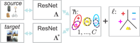
(a)

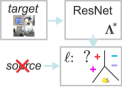
(b)

Figure 1: Supervised Domain Adaptation [22]. Figure 1(a): The source and target network streams are combined by the classification and alignment losses $\ell$ and $\hbar$ (end-to-end learning) which operate on the feature vectors from the final FC layers of ResNet-50 streams $\boldsymbol{\Lambda}$ and $\boldsymbol{\Lambda}^{*\!}$. Loss $\hbar$ aligns covariances for $C$ classes to facilitate transfer learning. Figure 1(b): At the test time, the target stream only and the classifier are used.

Supervised Domain Adaptation. In this paper, we employ the supervised domain adaptation which role is to transfer knowledge from the labeled source to labeled target dataset and outperform naive fine-tuning on combined datasets. We adapt an approach [22] based on the mixture of alignments of second-order statistics. One alignment per class per source and target streams is performed to discover the so-called commonality [22] between the data streams. Thus, both CNN streams learn a transformation of the data into this shared commonality. Figures 1(a) and 1(b) show the training and testing procedures. Training requires a trade-off between alignment and training losses $\hbar$ and $\ell$ operating on source and target streams $\boldsymbol{\Lambda}$ and $\boldsymbol{\Lambda}^{*\!}$. Testing uses only the target stream $\boldsymbol{\Lambda}^{*\!}$ and the pre-trained classifier.

Approach [22] assumes that the source and target data have to share the same set of labels. We relax this assumption to perform transfer between the classes shared between both datasets. Thus, we employ separate source and target classifiers and perform the alignment.

3 Preliminaries

In what follows, we explain our notations and the necessary background on shift-invariant RBF kernels and their linearization, which are needed for deriving a kernel on sequences on 3D body skeleton joints together with its linerization into feature maps.

Notations. The Kronecker product is denoted by $\otimes$. $\mathcal{I}_{N}$ denotes the index set $\left\{1,2,...,N\right\}$. We use the MATLAB notation $\boldsymbol{v}\!=\![\text{begin}\!:\!\text{step}\!:\!\text{end}]$ to generate a vector $\boldsymbol{v}$ with elements starting as begin, ending as end, with stepping equal step. Operator ‘;’ in $[\boldsymbol{x};\boldsymbol{y}]$ concatenates vectors $\boldsymbol{x}$ and $\boldsymbol{y}$ (or scalars) while $[\boldsymbol{\Phi}_{i}]_{i\in\mathcal{I}_{J}}$ concatenates $\boldsymbol{\Phi}_{1},...,\boldsymbol{\Phi}_{J}$ along rows.

Kernel Linearization. In the sequel, we use Gaussian kernel feature maps detailed below to embed 3D coordinates and their corresponding temporal time stamp into a non-linear Hilbert space and perform linearization which will result in our texture-like feature maps.

Proposition 1.

Let $G_{\sigma}(\boldsymbol{x}\!-\!\boldsymbol{y})=\exp(-\!\left\|{\boldsymbol{x}\!-\!\boldsymbol{y}}\right\|_{2}^{2}/{2\sigma^{2}})$ denote a Gaussian RBF kernel centered at $\boldsymbol{y}$ and having a bandwidth $\sigma$. Kernel linearization refers to rewriting this $G_{\sigma}$ as an inner-product of two infinite-dimensional feature maps. To obtain these maps, we use a fast approximation method based on probability product kernels [15]. Specifically, we employ the inner product of $d^{\prime}$-dimensional isotropic Gaussians given $\boldsymbol{x},\boldsymbol{y}\!\in\!\mathbb{R}^{d^{\prime}}\!$. Consider equation:

$$\!\!\!\!\!\!\!G_{\sigma}\!\left(\boldsymbol{x}\!-\!\boldsymbol{y}\right)\!\!=\!\!\left(\frac{2}{\pi\sigma^{2}}\right)^{\!\!\frac{d^{\prime}}{2}}\!\!\!\!\!\!\int\limits_{\boldsymbol{\zeta}\in\mathbb{R}^{d^{\prime}}}\!\!\!\!G_{\sigma/\sqrt{2}}\!\!\left(\boldsymbol{x}\!-\!\boldsymbol{\zeta}\right)G_{\sigma/\sqrt{2}}(\boldsymbol{y}\!\!-\!\boldsymbol{\zeta})\,\mathrm{d}\boldsymbol{\zeta}.$$ (1)

Eq. (1) can be approximated by replacing the integral with the sum over $Z$ pivots $\boldsymbol{\zeta}_{1},...,\boldsymbol{\zeta}_{Z}$:

$$\!\!\!\!\!\!\!G_{\sigma}(\boldsymbol{x}\!-\!\boldsymbol{y})\approx\left<\sqrt{c}\boldsymbol{\varphi}(\boldsymbol{x}),\sqrt{c}\boldsymbol{\varphi}(\boldsymbol{y})\right>,\text{ where }\boldsymbol{\varphi}(\boldsymbol{x})=\left[{G}_{\sigma/\sqrt{2}}(\boldsymbol{x}-\boldsymbol{\zeta}_{1}),...,{G}_{\sigma/\sqrt{2}}(\boldsymbol{x}-\boldsymbol{\zeta}_{Z})\right]^{T}\!\!,$$ (2)

and $c$ represents a constant (it impacts the overall magnitude only so we set $c\!=\!1$). We refer to (2) (left) as the linearization of the RBF kernel and (2) (right) as an RBF feature map.

Proof.

Rewrite the Gaussian kernel as the probability product kernel [15] (Sec. 3.1). ∎

4 Proposed Method

Below, we formulate the problem of action recognition from sequences of 3D body skeleton joints, followed by our kernel formulation capturing actions, and its linearization into feature maps which we further feed to off-the-shelf CNN for classification.

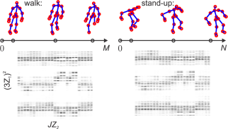
Figure 2: Visualization of the feature maps of sequences of 3D body skeleton joints. Note that irrespectively of the sequence length, we always obtain $\boldsymbol{\Phi}\!\in\!\mathbb{R}^{225\times 225}$ feature maps.

4.1 Generation of Feature Maps via Kernel Linearization

Let dataset consist of sequences of $J$ 3D body skeleton joints describing human pose skeleton evolving in time. For brevity, we assume each sequence consists of $M$ frames. However, our formulation is applicable to sequences of variable lengths e.g., $M$ and $N$. Our pose sequence $\Pi$ is defined as:

$$\Pi=\left\{\boldsymbol{x}_{is}\in\mathbb{R}^{3},i\in\mathcal{I}_{J},s\in\mathcal{I}_{M}\right\}.$$ (3)

Each sequence $\Pi$ is described by one of $C$ action labels. We use the sequence $\Pi$ to generate a feature map which can be considered a descriptor of action associated with $\Pi$. Then, such feature maps are generated from given datasets and then fed to the source and target CNN streams with the goal of performing the supervised domain adaptation. Figure 2 illustrates the sequences and feature maps obtained as a result of the process detailed next.

In what follows, we want to measure the similarity between any two action sequences in terms of their 3D body skeleton joints as well as their evolution in time. We normalize each skeleton w.r.t. the chest joint (chosen to be the center). Moreover, we normalize such relative coordinates by their total variance computed over the training data. Let $\Pi_{A}$ and $\Pi_{B}$ be two sequences, each with $J$ joints, and $M$ and $N$ frames, respectively. Further, let $\boldsymbol{x}_{is}\!\in\!\mathbb{R}^{3}$ and $\boldsymbol{y}_{jt}\!\in\!\mathbb{R}^{3}$ correspond to coordinates of joints of body skeletons of $\Pi_{A}$ and $\Pi_{B}$, respectively. We define our sequence kernel (SCK) between $\Pi_{A}$ and $\Pi_{B}$ as:

$$K(\Pi_{A},\Pi_{B})=\frac{1}{MN}\!\!\!\sum\limits_{i\in\mathcal{I}_{J}}\sum\limits_{s\in\mathcal{I}_{M}}\sum\limits_{t\in\mathcal{I}_{N}}\!K_{\sigma_{1}}\!\left(\boldsymbol{x}_{is}-\boldsymbol{y}_{it}\right)^{2}G_{\sigma_{2}}(\frac{s}{M}-\frac{t}{N}),$$ (4)

where $1/(MN)$ is a normalization constant, and $G_{\sigma_{1}}$ and $G_{\sigma_{2}}$ are subkernels that capture the similarity between the 3D body skeleton joints and temporal alignment, respectively. Therefore, we have two parameters $\sigma_{1}$ and $\sigma_{2}$ which control the level of tolerated invariance w.r.t. misalignment of 3D body joints and their temporal positions in two sequences, respectively. Moreover, the square of $K_{\sigma_{1}}$ in Eq. (4) captures co-occurrences of x, y, and z Cartesian coordinates of each 3D body joint–it is shown below that the square operation corresponds to the Kronecker product which is known to capture co-occurrences.

First, we define $K_{\sigma_{1}}(\boldsymbol{x}-\boldsymbol{y})\!=\!\sum_{i\in\mathcal{I}_{3}}G_{\sigma_{1}}(x^{i}-y^{i})$ where superscript $i$ chooses x-, y-, or z-axis of a 3D coordinate vector. Next, we linearize the above kernel using the theory from Section 3 so that $K_{\sigma_{1}}(\boldsymbol{x}-\boldsymbol{y})\!\approx\!\sum_{i\in\mathcal{I}_{3}}\phi(x^{i})^{T}\phi(y^{i})$, which gives the dot-product of concatenations $K_{\sigma_{1}}(\boldsymbol{x}-\boldsymbol{y})\!\approx\![\phi(x^{1});\phi(x^{2});\phi(x^{3})]^{T}[\phi(y^{1});\phi(y^{2});\phi(y^{3})]$. In what follows, we write for simplicity that $K_{\sigma_{1}}(\boldsymbol{x}-\boldsymbol{y})\!\approx\!\phi(\boldsymbol{x})^{T}\phi(\boldsymbol{y})$. Moreover, temporal kernel $G_{\sigma_{2}}(\frac{s}{M}-\frac{t}{N})\approx\boldsymbol{z}(s/M)^{T}\boldsymbol{z}(t/N)$. The above linearizations combined with Eq. (4) lead to:

$$K(\Pi_{A},\Pi_{B})\!\approx\!\frac{1}{MN}\!\!\sum\limits_{i\in\mathcal{I}_{J}}\sum\limits_{s\in\mathcal{I}_{M}}\!\sum\limits_{t\in\mathcal{I}_{N}}\!\!\!\big{(}\boldsymbol{\phi}(\boldsymbol{x}_{is})^{T}\boldsymbol{\phi}(\boldsymbol{y}_{it})\big{)}^{2}\boldsymbol{z}(s/M)^{T}\boldsymbol{z}(t/N),$$ (5)

which can be further rewritten into Eq. (6) and simplified by Eq. (7):

$$\!\!K(\Pi_{A},\Pi_{B})\!\approx\!\frac{1}{MN}\!\!\sum\limits_{i\in\mathcal{I}_{J}}\sum\limits_{s\in\mathcal{I}_{M}}\!\sum\limits_{t\in\mathcal{I}_{N}}\!\!\!\left<(\boldsymbol{\phi}(\boldsymbol{x}_{is})\!\otimes\!\boldsymbol{\phi}(\boldsymbol{x}_{is}))\boldsymbol{z}(s/M)^{T}\!\!,\,(\boldsymbol{\phi}(\boldsymbol{y}_{it})\!\otimes\!\boldsymbol{\phi}(\boldsymbol{y}_{it}))\boldsymbol{z}(t/N)^{T}\right>$$ (6)

$$\!\!\qquad\qquad\;=\sum\limits_{i\in\mathcal{I}_{J}}\!\!\Big{<}\!\frac{1}{M}\!\!\sum\limits_{s\in\mathcal{I}_{M}}\!\!(\boldsymbol{\phi}(\boldsymbol{x}_{is})\!\otimes\!\boldsymbol{\phi}(\boldsymbol{x}_{is}))\boldsymbol{z}(s/M)^{T}\!\!,\frac{1}{N}\!\!\sum\limits_{t\in\mathcal{I}_{N}}\!\!(\boldsymbol{\phi}(\boldsymbol{y}_{it})\!\otimes\!\boldsymbol{\phi}(\boldsymbol{y}_{it}))\boldsymbol{z}(t/N)^{T}\Big{>}\;\Rightarrow$$

$$\!\!K(\Pi_{A},\Pi_{B})\!\approx\!\left<\boldsymbol{\Phi}(\Pi_{A}),\boldsymbol{\Phi}(\Pi_{B})\right>,\;\text{where}$$ (7)

$$\!\!\boldsymbol{\Phi}(\Pi_{A})\!=\!\Big{[}\frac{1}{M}\!\!\sum\limits_{s\in\mathcal{I}_{M}}\!\!(\boldsymbol{\phi}(\boldsymbol{x}_{is})\!\otimes\!\boldsymbol{\phi}(\boldsymbol{x}_{is}))\boldsymbol{z}(s/M)^{T}\Big{]}_{i\in\mathcal{I}_{J}}\!,\boldsymbol{\Phi}(\Pi_{B})\!=\!\Big{[}\frac{1}{N}\!\!\sum\limits_{t\in\mathcal{I}_{N}}\!\!(\boldsymbol{\phi}(\boldsymbol{y}_{it})\!\otimes\!\boldsymbol{\phi}(\boldsymbol{y}_{it}))\boldsymbol{z}(t/N)^{T}\Big{]}_{i\in\mathcal{I}_{J}}\!,$$

and $\boldsymbol{\Phi}(\Pi)$ is our texture-like feat. map for a chosen sequence $\Pi$.

We choose $Z_{1}\!=\!5$ pivots pivots $\boldsymbol{\zeta}\!=\![\zeta_{1},...,\zeta_{Z_{1}}]^{T}$ for $G_{\sigma_{1}}$ which are sampled on interval $[-1;1]$ with equal steps e.g., $\boldsymbol{\zeta}\!=\![-1:2/(Z_{1}\!-\!1):1]$. This results in a $3Z_{1}$ dimensional map that approximates $K_{\sigma_{1}}$. For $G_{\sigma_{2}}$, we choose such an integer number of pivots $Z_{2}$ that $Z_{2}J\!=\!225$. We sample these pivots on interval $[0;1]$. This way, we obtain $\boldsymbol{\Phi}\!\in\!\mathbb{R}^{Z_{1}^{2}\times Z_{2}J}$ which can be readily fed to an off-the-shelf CNN stream. Figure 3 demonstrates the impact of $\sigma_{1}$ and $\sigma_{2}$ radii on the feature maps $\boldsymbol{\Phi}$.

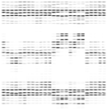
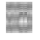
(a)

(b)

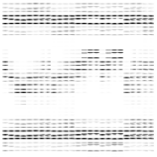
(c)

Figure 3: Illustration of the impact of $\sigma_{1}\!=\!0.4,0.6,0.8,1.5$ and $\sigma_{2}\!=\!0.02,0.1,1.0,5.0$ (in the scanline order) on feature maps are given in Figures 3(a) and 3(b), respectively. Figure 3(c) shows four different maps for four different sequences. Note the subtle differences.

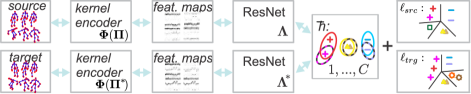
Figure 4: Our pipeline: combining the 3D body skeleton encoding and the supervised domain adaptation. Unlike [22], we utilize two classifiers (one per network stream) and perform alignment between the classes that are shared between the source and target datasets.

Our feature map is similar in spirit to Convolutional Kernel Networks [29] for image classification which demonstrated that the linearization of a carefully designed kernel adheres to standard CNN operations such as convolution, non-linearity and pooling. This motivates our belief that our feature maps are more suited/compatible for interfacing with CNNs than ad-hoc texture-like representations [19].

4.2 Alignment of Second-order Statistics

Our final pipeline is illustrated in Figure 4. As our ultimate goal is to transfer knowledge between Kinect-based datasets, we combine the described in Section 4.1 encoder of sequences of 3D body skeleton joints together with the supervised domain adaptation algorithm So-HoT [22]. Section 1 (supplementary material) details this algorithm. So-HoT yields state-of-the-art results on the Office dataset [35], however, it works with datasets which are described by the same class concepts. Thus, we adapt their algorithm to our particular needs e.g., we only perform the alignment of second-order statistics between the classes that are shared between the source and target datasets. Moreover, we employ separate classifier losses $\ell_{src}$ and $\ell_{trg}$ for the source and target stream, respectively. The separate target classifier allows the target network to work with class labels absent from the source dataset. At the test time, we cut off the source stream (and the source classifier), as illustrated in Figure 1(b).

Algorithm 1 (supplementary material) details how we perform domain adaptation. We enable the alignment loss $\hbar$ only if the source and target batches correspond to the same class. Otherwise, the alignment loss is disabled and the total loss uses only the classification log-losses $\ell_{src}$ and $\ell_{trg}$. To generate the source and target batches that match w.r.t. the class label, we re-order source and target datasets class-by-class and thus each source/target batch contains only one class label at a time. Once all source and target datapoints with matching class labels are processed, remaining datapoints are processed next. Lastly, we refer readers interested in the details of the So-HoT algorithm to paper [22] for specifics of the $\hbar$ loss.

5 Experiments

Below, we detail our network setting, datasets and we show experiments on our feature maps for sequences of 3D body skeleton joints in the context of the supervised domain adaptation.

Network Model. We use the two streams network architecture from [22]. For each CNN stream, we chose the Residual CNN model ResNet-50 [11] pre-trained on ImageNet dataset [24] for both source and target streams. The Pool-5 layers of the source and target streams are forwarded to a fully connected layer FC with 512 hidden units and this is forwarded to both the classification weight layer and the so-called alignment loss [22]. Two classifiers are used for the source and target streams. Moreover, the alignment loss is activated when the generated source and target mini-batches contain datapoints with the same class labels. See Algorithm 1 (supplementary material) for more details and Figure 4 for the network setting.

The training is performed by the Stochastic Gradient Descent (SGD) with the momentum set to 0.9. Mini-batch sizes differ depending on both the source and target dataset.

Datasets. We use the NTU RGB-D, SBUKinect Interaction and UTKinect-Action3D datasets.

NTU RGB-D [38], the largest action recognition dataset to date, contains $\sim$56000 sequences of 60 distinct action classes and sequences of actions/interactions performed by 40 different subjects. 3D coordinates of 25 body joints are provided. We use the cross-subject evaluation protocol [38] and used only the train split as our source data. For pre-processing, we translated 3D body joints by the joint-2 (middle of the spine) and we chose the body with the largest 3D motion as the main actor for the multi-actor sequences.

SBUKinect [47] contains videos of 8 interaction categories between two people, and 282 skeleton sequences with 15 3D body joints. Although the locations of body joints are noisy [47] and pre-processing is common [50], we do not perform any pre-processing or data augmentation in contrast to [19]. In domain adaptation setting, we use the NTU training set as the source and SBU as the target data. For evaluation, we follow [47] and use 5-fold cross-validation on the given splits. As each sequence contains 2 persons, we used each skeleton as a separate training datapoint. For testing, we averaged predictions over such pairs.

UTKinect-Action3D [44] contains 10 action captured by Kinect, 199 sequences, and 20 3D body skeleton joints.

Methods	SBU	UTK
Cylindrical textures, $1\!\times$CNN [19]	$89.37\%$	$95.0\%$
Cylindrical textures, $3\!\times$CNN [19]	$90.24\%$	$95.9\%$
Kernel feature maps, $1\!\times$CNN (ours)	$\bf 91.13\%$	$\bf 96.5\%$

Table 1: Comparisons of texture representations.

(a)

(b)

Figure 5: Accuracy w.r.t. $Z_{1}$ ($Z_{2}\!=\!15$) and $Z_{2}$ ($Z_{1}\!=\!5$) on SBU in Figures 5(a) and 5(b).

We avoid data augmentation or pre-processing. Protocol [51] has 2 splits: half of the subjects for training and half for testing. NTU training set is our source.

Experiments. Below, we focus on the following types of experiments, each utilizing our encoder which transforms sequences of 3D body skeleton joints into feature maps:

1. Target-only: only target dataset is used for training and testing (no domain adaptation).

2. Source+target: the source and target datasets (both training and validation splits) are combined into one larger dataset. Testing is performed on the target testing set only. No domain adaptation is used but the network is trained on both domains.

3. Second-order alignment: our extended So-HoT model applies the domain adaptation between the source and target training datapoints. We perform the alignment of second-order statistics whenever the source and target class names match.

Methods	Accuracy
Raw Skeleton [47]	$49.7\%$
Hierarchical RNN [7]	$80.35\%$
Deep LSTM [50]	$86.03\%$
Deep LSTM $+$ Co-occurrence [50]	$90.41\%$
ST-LSTM [27]	$88.6\%$
ST-LSTM $+$ Trust Gate [27]	$93.3\%$
Frames $+$ CNN [19]	$90.8\%$
Clips $+$ CNN $+$ MTLN [19]	$93.57\%$
SBU only (target)	91.13%
NTU+SBU combined (source+target)	91.52%
Second-order alignment	94.36%

Table 2: Results on the SBUKinect dataset.

Methods	Accuracy
3D Histogram (leave one out) [44]	$90.92\%$
Lie Group [42]	$97.08\%$
SCK $+$ DCK [21]	$98.39\%$
Skeleton Joint Features [51]	$90.9\%$
ST-LSTM $+$ Trust Gate [27]	$95.0\%$
Elastic Functional Coding [1]	$94.9\%$
UTK only (target)	$96.5\%$
NTU+UTK combined (source+target)	$97.5\%$
Second-order alignment	98.9%

Table 3: Results on the UTKinect dataset.

Methods	Cross subject
Hierarchical RNN [7]	$59.1\%$
Deep RNN [38]	$59.3\%$
Deep LSTM [38]	$60.7\%$
ST-LSTM $+$ Trust Gate [27]	$69.2\%$
Frames $+$ CNN [19]	${\bf 75.73}\%$
NTU only (target)	$74.52\%$
NTU+UTK+SBU combined (source+target)	$74.65\%$
Second-order alignment (UTK$\rightarrow$NTU)	$74.91\%$
Second-order alignment (SBU$\rightarrow$NTU)	$74.83\%$
Second-order alignment (UTK$+$SBU$\rightarrow$NTU)	${\bf 75.35\%}$

Table 4: Results on the NTU dataset.

(a)

(b)

Figure 6: Sensitivity w.r.t. param. $\sigma_{1}$ and $\sigma_{2}$ on SBU. Figures 6(a) and 6(b) show the accuracy w.r.t. $\sigma_{1}$ ($\sigma_{2}\!=\!0.3$) and $\sigma_{2}$ ($\sigma_{1}\!=\!0.6$), resp.

No Domain Adaptation. Firstly, we compare our encoding to texture-based representation [19]. Approach [19] forms 4 arrays of cylindrical coordinates of 3D skeleton body joints, each translated w.r.t. each 4 pre-defined key-joints. Such arrays are later resized, cropped etc. and fed to network via multiple CNN inputs. They require a dedicated CNN pipeline which combines all these arrays. To make a fairer comparison to our encoding and use an off-the-shelf CNN setting, we simplified representation [19] to use only a single body key-joint center for translation. We use the same setting for our encoding and [19] based on ResNet-50. We do not use a domain adaptation for results in Table 1. We include however a variant of method [19] which generates 3 texture images (one per each cylindrical coordinate). Thus, these 3 texture images are passed via 3 CNN streams and their FC vectors are concatenated.

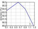
(a)

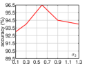
(b)

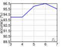
(c)

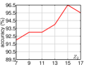
(d)

Figure 7: Sensitivity w.r.t. parameters $\sigma_{1}$ and $\sigma_{2}$ on UTK. Figures 7(a), 7(b), 7(c) and 7(d) show the accuracy w.r.t. $\sigma_{1}$ ($\sigma_{2}\!=\!0.6$), $\sigma_{2}$ ($\sigma_{1}\!=\!0.6$), $Z_{1}$ ($Z_{2}\!=\!15$) and $Z_{2}$ ($Z_{1}\!=\!5$), respectively.

Table 1 shows the comparison of our texture-like feature map encoding against method [19]. With $3\!\times$ more texture images taking $3\!\times$ more time to process via 3 CNN streams, method (Cylindrical textures, $3\!\times$CNN) [19] performs $\sim$0.7–0.9% worse than ours. Moreover, for fairness, we next combine their 3 texture images (one per each cylindrical coordinate) into an RGB-like texture and passed via 1 CNN stream (Cylindrical textures, $1\!\times$CNN). Table 1 shows that given the same ResNet-50 pipeline, our method outperforms theirs by $\sim$1.8% and 1.4% on SBU and UTK. Figures 1 and 7 show that our encoder is not too sensitive w.r.t. the choice of $Z_{1}$, $Z_{2}$, $\sigma_{1}$ and $\sigma_{2}$ on the SBU dataset (no domain adaptation). Figure 1 (supplementary material) shows a similar analysis on the UTK dataset.

Although idea [19] appears somewhat related to ours, the inner workings of both methods differ e.g., our method is mathematically inspired to attain desired shift-invariance w.r.t. 3D positions of coordinates and the temporal domain. In contrast, approach [19] is hand-crafted.

Domain Adaptation Setting. Having shown that our encoder outperforms [19] given the same pipeline, we discuss below results on the supervised domain adaptation pipeline.

In Table 3, we compare our method against state-of-the-art results on the SBU dataset. After enabling the domain adaptation algorithm (second-order alignment), the accuracy increases by 3.23% over training on the target data only (target). Our method also outperforms naive training on the combined source and target data (source+target) by 1.84%. We note that without any data augmentation, our method outperforms more complicated approaches which utilize numerous texture-like representations per sequence combined with several CNN streams and a fusion network (Clips+CNN+MTLN) [19]. This shows the effectiveness of our supervised domain adaptation on sequences of 3D body skeleton joints.

Table 3 shows on the UTK dataset that domain adaptation (second-order alignment) outperforms the baseline (target) and the naive fusion (source+target) by 2.4% and 1.4%.

Table 4 presents the transfer results from UTK and/or SBU to NTU. Transferring the knowledge from small- to large-scale datasets is a difficult task. However, by combining UTK and SBU to form a source dataset, we were able to still gain 0.8% improvement over the baseline (target). We obtain results similar to [19] with a much simpler pipeline.

6 Conclusions

In this paper, we have demonstrated that sequences of 3D body skeleton joints can be easily encoded with the use of appropriately designed kernel function. A linearization of such a kernel function produces texture-like feature maps which constitute a first feed-forward layer further interconnected with off-the-shelf CNNs. Moreover, we have also demonstrated that the supervised domain adaptation can be performed on such representations and that small-scale Kinect-based datasets can benefit from the knowledge transfer from the large-scale NTU dataset. We believe our contributions lead to state-of-the-art results. They also open up interesting avenues on how to use the time sequences with traditional off-the-shelf CNNs and how to leverage the abundance of the skeleton-based action recognition datasets.

Appendix A Supervised Domain Adaptation [22]

For the full details of the So-HoT algorithm, please refer to paper [22]. Below, we review the core part of their algorithm for the reader’s convenience. Suppose $\mathcal{I}_{N}$ and $\mathcal{I}_{N^{*}}\!$ are the indexes of $N$ source and $N^{*}\!$ target training data points. $\mathcal{I}_{N_{c}}$ and $\mathcal{I}_{N_{c}^{*}}\!$ are the class-specific indexes for $c\!\in\!\mathcal{I}_{C}$, where $C$ is the number of classes. Furthermore, suppose we have feature vectors from an FC layer of the source network stream, one per an action sequence or image, and their associated labels. Such pairs are given by $\boldsymbol{\Lambda}\!\equiv\!\{(\boldsymbol{\phi}_{n},y_{n})\}_{n\in\mathcal{I}_{N}}$, where $\boldsymbol{\phi}_{n}\!\in\!\mathbb{R}^{d}$ and $y_{n}\!\in\!\mathcal{I}_{C}$, $\forall n\!\in\!\mathcal{I}_{N}$. For the target data, by analogy, we define pairs $\boldsymbol{\Lambda}^{*\!}\!\equiv\!\{(\boldsymbol{\phi}^{*}_{n},y^{*}_{n})\}_{n\in\mathcal{I}_{N}^{*}}$, where $\boldsymbol{\phi}^{*}\!\!\in\!\mathbb{R}^{d}$ and $y^{*}_{n}\!\!\in\!\mathcal{I}_{C}$, $\forall n\!\in\!\mathcal{I}_{N}^{*}$. Class-specific sets of feature vectors are given as $\boldsymbol{\Phi}_{c}\!\equiv\!\{\boldsymbol{\phi}^{c}_{n}\}_{n\in\mathcal{I}_{N_{c}}}$ and $\boldsymbol{\Phi}_{c}^{*}\!\!\equiv\!\{\boldsymbol{\phi}^{*c}_{n}\}_{n\in\mathcal{I}_{N_{c}^{*}\!}}$, $\forall c\!\in\!\mathcal{I}_{C}$. Then $\boldsymbol{\Phi}\!\equiv\!(\boldsymbol{\Phi}_{1},...,\boldsymbol{\Phi}_{C})$ and $\boldsymbol{\Phi}^{*}\!\!\equiv\!(\boldsymbol{\Phi}^{*}_{1},...,\boldsymbol{\Phi}^{*}_{C})$. The asterisk in superscript (e.g. ${\boldsymbol{\phi}}^{*}$) denotes variables related to the target network while the source-related variables have no asterisk. Figure 4 shows the setup we use. The So-HoT problem is posed as a trade-off between the classifier and alignment losses $\ell$ and $\hbar$:

$$\!\!\!\!\!\!\!\!\!\!\!\!\!\!\!\!\!\!\operatorname*{arg\,min}\limits_{\;\;\begin{subarray}{c}\boldsymbol{W}\!,\boldsymbol{W}^{*}\!\!\!\!,\boldsymbol{\Theta},\boldsymbol{\Theta}^{*}\!\!\\ \;\;\;\;\text{s. t. }||\boldsymbol{\phi}_{n}||_{2}^{2}\leq\tau,\\ \;\;\;\;\;\;\;\;\,||\boldsymbol{\phi}^{*}_{n^{\prime}}||_{2}^{2}\leq\tau,\\ \;\;\;\;\forall n\in\mathcal{I}_{N}\!,n^{\prime}\!\in\mathcal{I}_{N}^{*}\end{subarray}}\ell\!\left(\boldsymbol{W}\!,\boldsymbol{\Lambda}\right)\!+\!\ell\!\left(\boldsymbol{W}^{*\!}\!,\boldsymbol{\Lambda}^{*\!}\right)\!+\!\eta||\boldsymbol{W}\!-\!\boldsymbol{W}^{*\!}||_{F}^{2}\;+$$ (8)

$$\qquad\qquad\quad\!\!\!\!\!\underbrace{\frac{\alpha_{1}}{C}\!\!\sum_{c\in\mathcal{I}_{C}}\!||\boldsymbol{\Sigma}_{c}\!-\!\boldsymbol{\Sigma}^{*}_{c}||_{F}^{2}\!+\!\!\frac{\alpha_{2}}{C}\!\!\sum_{c\in\mathcal{I}_{C}}\!||\boldsymbol{\mu}_{c}\!\!-\!\!\boldsymbol{\mu}_{c}^{*}||_{2}^{2}.}_{\hbar(\boldsymbol{\Phi},\boldsymbol{\Phi}^{*}\!)}\vspace{0.2cm}$$

For $\ell$, a generic Softmax loss is employed. For the source and target streams, the matrices $\boldsymbol{W},\boldsymbol{W}^{*}\!\!\in\!\mathbb{R}^{d\times C}$ contain unnormalized probabilities. In Equation (8), separating the class-specific distributions is addressed by $\ell$ while attracting the within-class scatters of both network streams is handled by $\hbar$. Variable $\eta$ controls the proximity between $\boldsymbol{W}$ and $\boldsymbol{W}^{*}\!$ which encourages the similarity between decision boundaries of classifiers.

The loss $\hbar$ depends on two sets of variables $(\boldsymbol{\Phi}_{1},...,\boldsymbol{\Phi}_{C})$ and $(\boldsymbol{\Phi}^{*}_{1},...,\boldsymbol{\Phi}^{*}_{C})$ – one set per network stream. Feature vectors $\boldsymbol{\Phi}(\boldsymbol{\Theta})$ and $\boldsymbol{\Phi}^{*}\!(\boldsymbol{\Theta}^{*}\!)$ depend on the parameters of the source and target network streams $\boldsymbol{\Theta}$ and $\boldsymbol{\Theta}^{*}\!$ that we optimize over. $\boldsymbol{\Sigma}_{c}\!\equiv\!\boldsymbol{\Sigma}(\boldsymbol{\Phi}_{c})$, $\boldsymbol{\Sigma}^{*}_{c}\!\equiv\!\boldsymbol{\Sigma}(\boldsymbol{\Phi}^{*}_{c})$, $\boldsymbol{\mu}_{c}(\boldsymbol{\Phi})$ and $\boldsymbol{\mu}^{*}_{c}(\boldsymbol{\Phi}^{*})$ denote the covariances and means, respectively, one covariance/mean pair per network stream per class. Coefficients $\alpha_{1}$, $\alpha_{2}$ control the degree of the scatter and mean alignment, $\tau$ controls the $\ell_{2}$-norm of feature vectors.

Appendix B Modifications to the So-HoT Approach

Algorithm 1 details how we perform domain adaptation. We enable the alignment loss $\hbar$ only if the source and target batches correspond to the same class. Otherwise, the alignment loss is disabled and the total loss uses only the classification log-losses $\ell_{src}$ and $\ell_{trg}$. To generate the source and target batches that match w.r.t. the class label, we re-order source and target datasets class-by-class and thus each source/target batch contains only one class label at a time. Once all source and target datapoints with matching class labels are processed, remaining datapoints are processed next. Lastly, we refer readers interested in the details of the So-HoT algorithm and loss $\hbar$ to paper [22].

Algorithm 1 Batch generation + a single epoch of the training procedure on the source and target datasets.

1:$src\_data:=\text{sort\_by\_class\_label}(src\_data)$

2:$target\_data:=\text{sort\_by\_class\_label}(target\_data)$

3:$C_{s}$$\triangleright$ Number of the source classes

4:$C_{t}$$\triangleright$ Number of the target classes

5:$C_{s\cap t}$$\triangleright$ Number of classes in common

6:procedure epoch($src\_data,target\_data,batch\_size$) $\triangleright$ Training (one epoch)

7:     for $i\leftarrow 1:max(C_{s},C_{t})$  do

8:         if $i\leq C_{s}$ then

9:              $batch_{s}\leftarrow\text{Choose}(src\_data,i,batch\_size)$ $\triangleright$ ‘Choose’ pre-fetches data of class i

10:         else

11:              $batch_{s}\leftarrow\text{Choose}(src\_data,rnd(),batch\_size)$ $\triangleright$ ‘Choose’ pre-fetches data of random class          

12:         if $i\leq C_{t}$ then

13:              $batch_{t}\leftarrow\text{Choose}(target\_data,i,batch\_size)$

14:         else

15:              $batch_{t}\leftarrow\text{Choose}(target\_data,rnd(),batch\_size)$          

16:         if $i\leq C_{s\cap t}$ then

17:              $Loss\leftarrow\ell_{src}+\ell_{trg}+\hbar$

18:         else

19:              $Loss\leftarrow\ell_{src}+\ell_{trg}$          

20:         Forward($net\_data$, $batch\_s$, $batch\_t$)

21:         Backward($net\_data$, $batch\_s$, $batch\_t$)

22:         Update($net\_data$, $batch\_s$, $batch\_t$)

References

- Anirudh et al. [2015] Rushil Anirudh, Pavan Turaga, Jingyong Su, and Anuj Srivastava. Elastic functional coding of human actions: From vector-fields to latent variables. In Proceedings of the IEEE Conference on Computer Vision and Pattern Recognition, pages 3147–3155, 2015.
- Bo et al. [2011] L Bo, K Lai, X Ren, and D Fox. Object recognition with hierarchical kernel descriptors. CVPR, 2011.
- Bobick and Davis [2001] Aaron F. Bobick and James W. Davis. The recognition of human movement using temporal templates. IEEE Transactions on pattern analysis and machine intelligence, 23(3):257–267, 2001.
- Cavazza et al. [2016] Jacopo Cavazza, Andrea Zunino, Marco San Biagio, and Murino Vittorio. Kernelized covariance for action recognition. CoRR abs/1604.06582, 2016.
- Collobert and Weston [2008] Ronan Collobert and Jason Weston. A unified architecture for natural language processing: Deep neural networks with multitask learning. In Proceedings of the 25th international conference on Machine learning, pages 160–167. ACM, 2008.
- Donahue et al. [2014] Jeff Donahue, Yangqing Jia, Oriol Vinyals, Judy Hoffman, Ning Zhang, Eric Tzeng, and Trevor Darrell. Decaf: A deep convolutional activation feature for generic visual recognition. In International conference on machine learning, pages 647–655, 2014.
- Du et al. [2015] Yong Du, Wei Wang, and Liang Wang. Hierarchical recurrent neural network for skeleton based action recognition. In Proceedings of the IEEE conference on computer vision and pattern recognition, pages 1110–1118, 2015.
- Feichtenhofer et al. [2016] Christoph Feichtenhofer, Axel Pinz, and Richard P. Wildes. Spatiotemporal residual networks for video action recognition. NIPS, 2016.
- Gaidon et al. [2011] Adrien Gaidon, Zaid Harchoui, and Cordelia Schmid. A time series kernel for action recognition. BMVC, pages 63.1–63.11, 2011.
- Girshick et al. [2014] Ross Girshick, Jeff Donahue, Trevor Darrell, and Jitendra Malik. Rich feature hierarchies for accurate object detection and semantic segmentation. In The IEEE Conference on Computer Vision and Pattern Recognition (CVPR), June 2014.
- He et al. [2016] Kaiming He, Xiangyu Zhang, Shaoqing Ren, and Jian Sun. Deep residual learning for image recognition. CVPR, 2016.
- Herath et al. [2017] Samitha Herath, Mehrtash Harandi, and Fatih Porikli. Going deeper into action recognition: A survey. Image and Vision Computing, 60:4–21, 2017.
- Hinton et al. [2012] Geoffrey Hinton, Li Deng, Dong Yu, George E Dahl, Abdel-rahman Mohamed, Navdeep Jaitly, Andrew Senior, Vincent Vanhoucke, Patrick Nguyen, Tara N Sainath, et al. Deep neural networks for acoustic modeling in speech recognition: The shared views of four research groups. IEEE Signal Processing Magazine, 29(6):82–97, 2012.
- Hussein et al. [2013] M. E. Hussein, M. Torki, M. Gowayyed, and M. El-Saban. Human action recognition using a temporal hierarchy of covariance descriptors on 3D joint locations. IJCAI, pages 2466–2472, 2013.
- Jebara et al. [2004] T. Jebara, R. Kondor, and A. Howard. Probability product kernels. JMLR, 5:819–844, 2004.
- Ji et al. [2013] Shuiwang Ji, Wei Xu, Ming Yang, and Kai Yu. 3d convolutional neural networks for human action recognition. IEEE transactions on pattern analysis and machine intelligence, 35(1):221–231, 2013.
- Johansson [1973] G. Johansson. Visual perception of biological motion and a model for its analysis. Perception and Psychophysics, 14(2):201–211, 1973.
- Karpathy et al. [2014] Andrej Karpathy, George Toderici, Sanketh Shetty, Thomas Leung, Rahul Sukthankar, and Li Fei-Fei. Large-scale video classification with convolutional neural networks. In Proceedings of the IEEE conference on Computer Vision and Pattern Recognition, pages 1725–1732, 2014.
- Ke et al. [2017] Qiuhong Ke, Mohammed Bennamoun, , Senjian An, Ferdous Sohel, and Farid Boussaid. A new representation of skeleton sequences for 3d action recognition. CVPR, 2017.
- Klaser et al. [2008] Alexander Klaser, Marcin Marszałek, and Cordelia Schmid. A spatio-temporal descriptor based on 3d-gradients. In BMVC 2008-19th British Machine Vision Conference, pages 275–1. British Machine Vision Association, 2008.
- Koniusz et al. [2016] P. Koniusz, A. Cherian, and F. Porikli. Tensor representations via kernel linearization for action recognition from 3D skeletons. ECCV, 2016.
- Koniusz et al. [2017] Piotr Koniusz, Yusuf Tas, and Fatih Porikli. Domain adaptation by mixture of alignments of second- or higher-order scatter tensors. CVPR, 2017.
- Krizhevsky et al. [2012a] Alex Krizhevsky, Ilya Sutskever, and Geoffrey E Hinton. Imagenet classification with deep convolutional neural networks. In Advances in neural information processing systems, pages 1097–1105, 2012a.
- Krizhevsky et al. [2012b] Alex Krizhevsky, Ilya Sutskever, and Geoffrey E Hinton. Imagenet classification with deep convolutional neural networks. In Advances in neural information processing systems, pages 1097–1105, 2012b.
- Kuehne et al. [2011] Hildegard Kuehne, Hueihan Jhuang, Estíbaliz Garrote, Tomaso Poggio, and Thomas Serre. Hmdb: a large video database for human motion recognition. In Computer Vision (ICCV), 2011 IEEE International Conference on, pages 2556–2563. IEEE, 2011.
- Laptev [2005] Ivan Laptev. On space-time interest points. International journal of computer vision, 64(2-3):107–123, 2005.
- Liu et al. [2016] Jun Liu, Amir Shahroudy, Dong Xu, and Gang Wang. Spatio-temporal lstm with trust gates for 3d human action recognition. In European Conference on Computer Vision, pages 816–833. Springer, 2016.
- Lv and Nevatia [2006] F. Lv and R. Nevatia. Recognition and segmentation of 3-D human action using hmm and multi-class adaboost. ECCV, pages 359–372, 2006. doi: 10.1007/11744085˙28.
- Mairal et al. [2014] J. Mairal, P. Koniusz, Z. Harchaoui, and C. Schmid. Convolutional kernel networks. NIPS, 2014.
- Ofli et al. [2014] F. Ofli, R. Chaudhry, G. Kurillo, R. Vidal, and R. Bajcsy. Sequence of the most informative joints (SMIJ). J. Vis. Comun. Image Represent., 25(1):24–38, 2014. ISSN 1047-3203. doi: 10.1016/j.jvcir.2013.04.007.
- Ohn-Bar and Trivedi [2013] E. Ohn-Bar and M. M. Trivedi. Joint angles similarities and HOG2 for action recognition. CVPR Workshop, 2013.
- Parameswaran and Chellappa [2006] V. Parameswaran and R. Chellappa. View invariance for human action recognition. IJCV, 66(1):83–101, 2006. doi: 10.1007/s11263-005-3671-4.
- Presti and La Cascia [2015] Liliana Lo Presti and Marco La Cascia. 3D skeleton-based human action classification: A survey. Pattern Recognition, 2015.
- Ren et al. [2015] Shaoqing Ren, Kaiming He, Ross Girshick, and Jian Sun. Faster r-cnn: Towards real-time object detection with region proposal networks. In Advances in neural information processing systems, pages 91–99, 2015.
- Saenko et al. [2010] Kate Saenko, Brian Kulis, Mario Fritz, and Trevor Darrell. Adapting visual category models to new domains. In European conference on computer vision, pages 213–226. Springer, 2010.
- Scholkopf and Smola [2001] Bernhard Scholkopf and Alexander J. Smola. Learning with Kernels: Support Vector Machines, Regularization, Optimization, and Beyond. MIT Press, Cambridge, MA, USA, 2001. ISBN 0262194759.
- Schuldt et al. [2004] Christian Schuldt, Ivan Laptev, and Barbara Caputo. Recognizing human actions: a local svm approach. In Pattern Recognition, 2004. ICPR 2004. Proceedings of the 17th International Conference on, volume 3, pages 32–36. IEEE, 2004.
- Shahroudy et al. [2016] Amir Shahroudy, Jun Liu, Tian-Tsong Ng, and Gang Wang. Ntu rgb+ d: A large scale dataset for 3d human activity analysis. In Proceedings of the IEEE Conference on Computer Vision and Pattern Recognition, pages 1010–1019, 2016.
- Shotton et al. [2013] Jamie Shotton, Toby Sharp, Alex Kipman, Andrew Fitzgibbon, Mark Finocchio, Andrew Blake, Mat Cook, and Richard Moore. Real-time human pose recognition in parts from single depth images. Communications of the ACM, 56(1):116–124, 2013.
- Simonyan and Zisserman [2014] Karen Simonyan and Andrew Zisserman. Two-stream convolutional networks for action recognition in videos. In Advances in neural information processing systems, pages 568–576, 2014.
- Tzeng et al. [2015] E. Tzeng, J. Hoffman, T. Darrell, and K. Saenko. Simultaneous deep transfer across domains and tasks. ICCV, pages 4068–4076, 2015.
- Vemulapalli et al. [2014] Raviteja Vemulapalli, Felipe Arrate, and Rama Chellappa. Human action recognition by representing 3D skeletons as points in a Lie Group. CVPR, pages 588–595, 2014. doi: http://doi.ieeecomputersociety.org/10.1109/CVPR.2014.82.
- Wu et al. [2012] Y. Wu, Z. Liu, Y. Wu, and J. Yuan. Mining actionlet ensemble for action recognition with depth cameras. CVPR, pages 1290–1297, 2012.
- Xia et al. [2012] Lu Xia, Chia-Chih Chen, and JK Aggarwal. View invariant human action recognition using histograms of 3d joints. In Computer Vision and Pattern Recognition Workshops (CVPRW), 2012 IEEE Computer Society Conference on, pages 20–27. IEEE, 2012.
- Yacoob and Black [1998] Y. Yacoob and M. J. Black. Parameterized modeling and recognition of activities. ICCV, pages 120–128, 1998.
- Yang and Tian [2014] X. Yang and Y. Tian. Effective 3D action recognition using eigenjoints. J. Vis. Comun. Image Represent., 25(1):2–11, 2014. ISSN 1047-3203. doi: 10.1016/j.jvcir.2013.03.001.
- Yun et al. [2012] Kiwon Yun, Jean Honorio, Debaleena Chattopadhyay, Tamara L Berg, and Dimitris Samaras. Two-person interaction detection using body-pose features and multiple instance learning. In Computer Vision and Pattern Recognition Workshops (CVPRW), 2012 IEEE Computer Society Conference on, pages 28–35. IEEE, 2012.
- Zatsiorsky [1997] V. M. Zatsiorsky. Kinematic of human motion. Human Kinetics Publishers, 1997.
- Zeiler and Fergus [2014] Matthew D Zeiler and Rob Fergus. Visualizing and understanding convolutional networks. In European conference on computer vision, pages 818–833. Springer, 2014.
- Zhu et al. [2016] Wentao Zhu, Cuiling Lan, Junliang Xing, Wenjun Zeng, Yanghao Li, Li Shen, Xiaohui Xie, et al. Co-occurrence feature learning for skeleton based action recognition using regularized deep lstm networks. In AAAI Conference on Artificial Intelligence, 2016.
- Zhu et al. [2013] Yu Zhu, Wenbin Chen, and Guodong Guo. Fusing spatiotemporal features and joints for 3d action recognition. In Computer vision and pattern recognition workshops (CVPRW), 2013 IEEE conference on, pages 486–491. IEEE, 2013.