Beyond Backprop: Online Alternating Minimization with Auxiliary Variables

Abstract

Despite significant recent advances in deep neural networks, training them remains a challenge due to the highly non-convex nature of the objective function. State-of-the-art methods rely on error backpropagation, which suffers from several well-known issues, such as vanishing and exploding gradients, inability to handle non-differentiable nonlinearities and to parallelize weight-updates across layers, and biological implausibility. These limitations continue to motivate exploration of alternative training algorithms, including several recently proposed auxiliary-variable methods which break the complex nested objective function into local subproblems. However, those techniques are mainly offline (batch), which limits their applicability to extremely large datasets, as well as to online, continual or reinforcement learning. The main contribution of our work is a novel online (stochastic/mini-batch) alternating minimization (AM) approach for training deep neural networks, together with the first theoretical convergence guarantees for AM in stochastic settings and promising empirical results on a variety of architectures and datasets.

1 Introduction

Backpropagation (backprop) (Rumelhart et al., 1986) has been the workhorse of neural net learning for several decades, and its practical effectiveness is demonstrated by recent successes of deep learning in a wide range of applications. Backprop (chain rule differentiation) is used to compute gradients in state-of-the-art learning algorithms such as stochastic gradient descent (SGD) (Robbins & Monro, 1985) and its variations (Duchi et al., 2011; Tieleman & Hinton, 2012; Zeiler, 2012; Kingma & Ba, 2014).

However, backprop has several drawbacks as well, including the commonly known vanishing gradient issue, resulting from recursive application of the chain rule through multiple layers of deep and/or recurrent networks (Bengio et al., 1994; Riedmiller & Braun, 1993; Hochreiter & Schmidhuber, 1997; Pascanu et al., 2013; Goodfellow et al., 2016). Although several approaches were proposed to address this issue, including Long Short-Term Memory (Hochreiter & Schmidhuber, 1997), RPROP (Riedmiller & Braun, 1993), and rectified linear units (ReLU) (Nair & Hinton, 2010), the fundamental problem with computing gradients of a deeply nested objective function remains. Moreover, backpropagation does not apply directly to non-differentiable nonlinearities and does not allow parallel weight updates across the layers (Le et al., 2011; Carreira-Perpiñán & Wang, 2014; Taylor et al., 2016).

Also, besides its computational issues, backprop is often criticized from a neuroscience perspective as a biologically implausible learning mechanism (Lee et al., 2015; Bartunov et al., 2018; Krotov & Hopfield, 2019; Sacramento et al., 2018; Guerguiev et al., 2017), due to multiple factors including the need for "a distinct form of information propagation (error feedback) that does not influence neural activity, and hence does not conform to known biological feedback mechanisms underlying neural communication" (Bartunov et al., 2018).

The issues mentioned above continue to motivate research on alternative algorithms for neural net learning. Several approaches were proposed recently, introducing auxiliary variables associated with hidden unit activations in order to decompose the highly coupled problem of optimizing a nested loss function into multiple, loosely coupled, simpler subproblems. These include alternating direction method of multipliers (ADMM) (Taylor et al., 2016; Zhang et al., 2016) and alternating-minimization or block coordinate descent (BCD) methods (Carreira-Perpiñán & Wang, 2014; Zhang & Brand, 2017; Zhang & Kleijn, 2017; Askari et al., 2018; Zeng et al., 2018; Lau et al., 2018; Gotmare et al., 2018).

A similar formulation, using Lagrange multipliers, was proposed earlier in (LeCun, 1986, 1987; LeCun et al., 1988), where a constrained formulation involving activations required the output of the previous layer to be equal to the input of the next layer, leading to the target propagation algorithm and recent extensions (Lee et al., 2015; Bartunov et al., 2018) (unlike BCD and ADMM, target prop uses layer-wise inverses of the forward mappings). These methods are viewed as somewhat more bio-plausible alternatives to backprop due to explicit propagation of (noisy/nondeterministic) neuronal activity and (layer-)local synaptic updates (see (Bartunov et al., 2018) for details). Note that the above bio-plausibility arguments are equally applicable to auxiliary-variable methods based on explicit optimization of (noisy) neural activations, and breaking the weight update problem into local, layer-wise optimization subproblems.

In this paper, we propose a novel activation-propagation approach, which, similarly to prior BCD and ADMM approaches, performs alternating minimization of network weights and auxiliary activation variables. However, unlike those methods, which all assume an offline (batch) setting and require the full training dataset at each iteration, our method is an online, incremental learning approach, that performs stochastic (minibatch) alternating minimization (AM). Two variants of AM are proposed, AM-Adam and AM-mem, which use different approaches for optimizing local subproblems.

Note that, unlike ADMM-based methods (Taylor et al., 2016; Zhang et al., 2016) and some previously proposed BCD methods (Zeng et al., 2018), our approach does not require Lagrange multipliers and only uses one set of auxiliary variables per layer: it is as memory-efficient as standard SGD, which stores activation values for gradient computations. The same distinction, along with multiple others (discussed in Supplementary Material), exists between our method and another recently proposed alternating-minimization scheme, ProxProp (Thomas Frerix, 2018). Also, we assume arbitrary loss functions and nonlinearities (unlike, for example, (Zhang & Brand, 2017) which assumes ReLU nonlinearities), and perform extensive empirical evaluation beyond the fully-connected networks, commonly used to evaluate auxiliary-variable methods.

In summary, our contributions include:

• algorithm(s): a novel online (mini-batch) auxiliary-variable approach for training neural networks without the gradient chain rule of backprop; unlike prior offline (batch) auxiliary-variable algorithms, our method can scale to arbitrarily large datasets and is applicable in continual and reinforcement learning settings;

• theory: to the best of our knowledge, we propose the first general theoretical convergence guarantees of alternating minimization in the stochastic setting. We show that the error of AM decays at the sub-linear rate $O((1/t)^{3/2}+1/t)$ as a function of the iteration $t$;

• extensive empirical evaluation on a variety of network architectures and datasets, demonstrating significant advantages of our method vs. offline counterparts, as well as somewhat faster initial convergence as compared to SGD and Adam, followed by similar asymptotic performance;

• our online method inherits common advantages of similar offline auxiliary-variable methods, including (1) no vanishing gradients, (2) handling of non-differentiable nonlinearities more easily in local subproblems, and (3) the possibility for parallelizing weight updates across layers;

• similarly to target propagation approaches (LeCun, 1986, 1987; Lee et al., 2015; Bartunov et al., 2018), our method is based on an explicit propagation of neural activity and local synaptic updates, which is one step closer to a more biologically plausible credit assignment mechanism than backprop; see (Bartunov et al., 2018) for a detailed discussion on this topic.

2 Alternating Minimization: Breaking Gradient Chains with Auxiliary Variables

We denote as $(\boldsymbol{X},\boldsymbol{Y})=$ $\{(\boldsymbol{x}_{1},\boldsymbol{y}_{1}),...,(\boldsymbol{x}_{n},\boldsymbol{y}_{n})\}$ a dataset of $n$ labeled samples, where $\boldsymbol{x}_{t}$ and $\boldsymbol{y}_{t}$ are the sample and its (vector) label at time $t$, respectively (e.g., one-hot $m$-dimensional vector $\boldsymbol{y}$ encoding discrete labels with $m$ possible values). We assume $\boldsymbol{x}\in\mathbb{R}^{N}$, and $\boldsymbol{y}\in\{0,1\}^{m}$. Given a fully-connected neural network with $L$ hidden layers, $\boldsymbol{W^{j}}$ denotes the $m_{j}\times m_{j-1}$ link weight matrix associated with the links from layer $j-1$ to layer $j$, where $m_{j}$ is the number of nodes at layer $j$. $\boldsymbol{W}^{L+1}$ denotes the $m_{L}\times m$ weight matrix connecting the last hidden layer $L$ with the output. We denote the set of all weights $\boldsymbol{W}=\{\boldsymbol{W}^{1},...,\boldsymbol{W}^{L+1}\}$.

Optimization problem. Training a fully-connected neural network with $L$ hidden layers consists of minimizing, with respect to weights ${\boldsymbol{W}}$, the loss ${\cal{L}}(y,f({\boldsymbol{W}},\boldsymbol{x}_{L}))$ involving a nested function $f({\boldsymbol{W}},\boldsymbol{x}_{L})=f_{L+1}(\boldsymbol{W}_{L+1},f_{L}(\boldsymbol{W}_{L},f_{L-1}(\boldsymbol{W}_{L-1},...f_{1}(\boldsymbol{W}_{1},\boldsymbol{x})...)$; this can be re-written as constrained optimization:

$$\min_{\boldsymbol{W}} \sum_{t=1}^{n}{\cal{L}}(\boldsymbol{y}_{t},\boldsymbol{a}_{t}^{L},\boldsymbol{W}^{L+1}),~{}where~{}\boldsymbol{a}_{t}^{l}=\sigma_{l}(\boldsymbol{c}^{l}_{t}),$$ (1)

$$s.t.~{}\boldsymbol{c}^{l}_{t}=\boldsymbol{W}^{l}\boldsymbol{a}_{t}^{l-1},~{}l=1,...,L,~{}and~{}~{}\boldsymbol{a_{t}}^{0}=\boldsymbol{x}_{t}.$$

In the above formulation, we use $\boldsymbol{a}_{t}^{l}$ as shorthand (not a new variable) denoting the activation vector of hidden units in layer $l$, where $\sigma$ is a nonlinear activation function (e.g, ReLU, $tanh$, etc) applied to code $\boldsymbol{c}^{l}$, a new auxiliary variable that must be equal to a linear transformation of the previous-layer activations.

For classification problems, we use the multinomial loss as our objective function:  ${\cal{L}}(\boldsymbol{y},\boldsymbol{x},\boldsymbol{W})=-\log{P(\boldsymbol{y}|\boldsymbol{x},\boldsymbol{W})}$

$$\begin{array}[]{ll}=&-\displaystyle\sum_{i=1}^{m}{\boldsymbol{y}_{i}(\boldsymbol{w}_{i}^{T}\boldsymbol{x})}+\log{(\displaystyle\sum_{l=1}^{m}{\exp{(\boldsymbol{w}_{l}^{T}\boldsymbol{x})}})},\end{array}\vspace{-0.02in}$$ (2)

where $w_{i}$ is the $i^{th}$ column of $\boldsymbol{W}$, $y_{i}$ is the $i^{th}$ entry of the one-hot vector encoding $\boldsymbol{y}$, and the class likelihood is modeled as $P(y_{i}=1|\boldsymbol{x},\boldsymbol{W})=$ $\exp{(\boldsymbol{w}_{i}^{T}\boldsymbol{x})}/\sum_{l=1}^{m}{\exp{(\boldsymbol{w}_{l}^{T}\boldsymbol{x})}}$.

Offline Alternating Minimization. We start with an offline optimization problem formulation, for a given dataset of $n$ samples, which is similar to (Carreira-Perpiñán & Wang, 2014) but uses multinomial instead of quadratic loss, and a different set of auxiliary variables. Namely, we use the following relaxation of the constrained formulation in eq. 1:

$$\begin{split}f(\boldsymbol{W},\boldsymbol{C})&=\sum_{t=1}^{n}{\cal{L}}(y_{t},\sigma_{L}(\boldsymbol{c}_{t}^{L}),\boldsymbol{W}^{L+1})\\ &\quad+\mu\sum_{t=1}^{n}\sum_{l=1}^{L}||\boldsymbol{c}_{t}^{l}-\boldsymbol{W}^{l}\sigma_{l-1}(\boldsymbol{c}_{t}^{l-1})||_{2}^{2}.\end{split}$$ (3)

This problem can be solved by alternating minimization (AM), or block-coordinate descent (BCD), over weights $\boldsymbol{W}=\{\boldsymbol{W}^{1},...,\boldsymbol{W}^{L+1}\}$ and codes $\boldsymbol{C}=\{\boldsymbol{c}_{1}^{1},...,\boldsymbol{c}_{1}^{L},$ $...\boldsymbol{c}_{n}^{1},...,\boldsymbol{c}_{n}^{L},\}$. Each iteration involves optimizing $\boldsymbol{W}$ for fixed $\boldsymbol{C}$, followed by fixing $\boldsymbol{W}$ and optimizing $\boldsymbol{C}$. The parameter $\mu>0$ acts as a regularization weight. As in (Carreira-Perpiñán & Wang, 2014), we use an adaptive scheme for gradually increasing $\mu$ over iterations

Online Alternating Minimization. The offline alternating minimization outlined above is not scalable to extremely large datasets (even data-parallel methods, such as (Taylor et al., 2016), are inherently limited by the number of cores available), and not suitable for incremental, continual/lifelong (Ring, 1994; Thrun, 1995, 1998) or reinforcement learning scenarios with potentially infinite data streams. To overcome those limitations, we propose a general online AM algorithmic scheme and present two specific algorithms which differ in optimization approaches used for updating $\boldsymbol{W}$; both algorithms are later evaluated and compared empirically.

Our approach is outlined in Algorithms 1, 2, and 3, omitting implementation details such as the adaptive $\mu$ schedule, hyperparameters controlling the number of iterations in optimization subroutines, and several others; we will make our code available online. As an input, the method takes an initial $\boldsymbol{W}$ (e.g., random), initial penalty weight $\mu$, learning rate for the predictive layer, $\eta$, and a Boolean variable $Mem$, indicating which optimization method to use for $\boldsymbol{W}$ updates; if $Mem=1$, a memory-based approach (discussed below) is selected, and initial memory matrices $\boldsymbol{A_{0}}$, $\boldsymbol{B_{0}}$ (described below) will be provided (typically, both are initialized to all zeros unless we want to retain the memory of some prior learning experience, e.g. in a continual learning scenario). The algorithm processes samples one at a time (but can easily be generalized to mini-batches); the current sample is encoded in its representations at each layer (encodeInput procedure, Algorithm 2), and an output prediction is made based on such encodings. The prediction error is computed, and the backward code updates follow as shown in the updateCodes procedure, where the code vector at layer $l$ is optimized with respect to the only two parts of the global objective that the code variables participate in. Once the codes are updated, the weights can be optimized in parallel across the layers (in updateWeights procedure, Algorithm 3) since fixing codes breaks the weight optimization problem into layer-wise independent subproblems. We next discuss each step in detail.

Algorithm 1 Online Alternating Minimization (AM)

0:  $(\boldsymbol{x},\boldsymbol{y})\sim p(\boldsymbol{x},y)$ (data stream sampled from distribution $p(\boldsymbol{x},\boldsymbol{y})$; initial weights $\boldsymbol{W}_{0}$; $\mu\in\mathbb{R^{+}}$ (quadratic penalty weight); $\eta\in\mathbb{R^{+}}$ (top-layer weight update step size); $Mem$ (indicates the type of optimization method for updateWeights; if "yes", input initial memory matrices $\boldsymbol{A_{0}}$ and $\boldsymbol{B_{0}}$).

1:  while more samples do

2:    Input $(\boldsymbol{x}_{t},y_{t})$

3:    $\boldsymbol{C}\leftarrow$ encodeInput($~{}\boldsymbol{x}_{t}$,$~{}\boldsymbol{W}_{t-1}$) % forward: compute linear activations at layers $1,...,L$

4:    $\boldsymbol{C}\leftarrow$ updateCodes($~{}\boldsymbol{C}$,$~{}y_{t}$, $~{}\boldsymbol{W}_{t-1}$,$~{}\mu$) % backward: error propagation by activation (code) changes

5:    $\boldsymbol{W}_{t}\leftarrow\mbox{\bf updateWeights}(~{}\boldsymbol{W}_{t-1},~{}\boldsymbol{x}_{t},~{}y_{t},~{}\boldsymbol{C},~{}\mu,~{}\eta,~{}Mem$)

6:  end while

7:  return $\boldsymbol{W}_{t}$

Algorithm 2 Activation Propagation (Code Update) Steps

encodeInput($~{}\boldsymbol{x}$,$~{}\boldsymbol{W}$)

1:  $\boldsymbol{c}^{0}=\boldsymbol{x}$

2:  for $l=1$ to $L$ do

3:    $\boldsymbol{c}^{l}=\boldsymbol{W}^{l}\sigma_{l-1}(\boldsymbol{c}^{l-1})$% $\sigma_{0}(\boldsymbol{x})=\boldsymbol{x},\sigma_{l}(\boldsymbol{x})=ReLU(\boldsymbol{x})~{}for~{}l=1,...,L$

4:  end for

5:  return $\boldsymbol{C}$

updateCodes($~{}\boldsymbol{C}$,$~{}\boldsymbol{y}$,$~{}\boldsymbol{W}$,$~{}\lambda_{C}$,$~{}\mu$)

1:  $\boldsymbol{c}^{L}\leftarrow\text{Solve Problem}$ (4), $~{}~{}\boldsymbol{c}^{0}=\boldsymbol{x}$

2:  for $l=L-1$ to $1$ do

3:    $\boldsymbol{c}^{l}\leftarrow\text{Solve Problem}$ (5)

4:  end for

5:  return $\boldsymbol{C}$

Algorithm 3 Weight and Memory Update Steps

updateWeights$(~{}\boldsymbol{W},~{}\boldsymbol{x},~{}y,~{}\boldsymbol{C},~{}\mu,~{}\eta,~{}Mem)$

1:  $\boldsymbol{W}^{L+1}=\boldsymbol{W^{L+1}}-\eta\nabla_{\boldsymbol{W}}{\cal{L}}(y,\sigma_{L}(\boldsymbol{c}^{L}),\boldsymbol{W^{L+1}})$

2:  for $l=1$ to $L$ do

3:    if $Mem$ then

4:       $(\boldsymbol{A^{l}}_{t},\boldsymbol{B^{l}}_{t})\leftarrow$ $\mbox{\bf updateMemory}(~{}\boldsymbol{A^{l}}_{t-1}$, $~{}\boldsymbol{B^{l}}_{t-1}$,$~{}\boldsymbol{C^{l}}$)

5:       % $\hat{f}^{l}(\boldsymbol{W^{l}})\equiv Tr(\boldsymbol{W}^{T}\boldsymbol{W}\boldsymbol{A}^{l})-2Tr(\boldsymbol{W}^{T}\boldsymbol{B}^{l})$

6:       $\boldsymbol{W}^{l}=\arg\min_{W}\hat{f}^{l}(\boldsymbol{W})$

7:    else

8:       %(parallel) local update of each layer weights,

9:       %(independently of other layers (unlike backprop)

10:       $\boldsymbol{W}^{l}\leftarrow$ $\mbox{\bf SGD}(~{}\boldsymbol{W^{l}},~{}\boldsymbol{x},~{}y,~{}\boldsymbol{C^{l}},~{}\mu,~{}\eta)$

11:    end if

12:  end for

13:  return $\boldsymbol{W}$

updateMemory($~{}\boldsymbol{A}$, $~{}\boldsymbol{B}$,$~{}\boldsymbol{C}$)

1:  for $l=1$ to $L$ do

2:    $\boldsymbol{a}=\sigma_{l-1}(\boldsymbol{c}^{l-1})$, $~{}\boldsymbol{A}^{l}\leftarrow\boldsymbol{A}^{l}+\boldsymbol{a}\boldsymbol{a}^{T}$, $~{}\boldsymbol{B}^{l}\leftarrow\boldsymbol{B}^{l}+\boldsymbol{c}^{l}\boldsymbol{a}^{T}$

3:  end for

4:  return $\boldsymbol{A},\boldsymbol{B}$

Activation propagation: forward and backward passes. In an online setting, we only have access to the current sample $\boldsymbol{x}_{t}$ at time $t$, and thus can only compute the corresponding codes $\boldsymbol{c}_{t}^{l}$ using the weights computed so far. Namely, given input $\boldsymbol{x}_{t}$, we compute the last-layer activations $\boldsymbol{a}_{t}^{L}=\sigma_{L}(\boldsymbol{c}^{L}_{t})$ in a forward pass, propagating activations from input to the last layer, and make a prediction about $y_{t}$, incurring the loss ${\cal{L}}(y_{t},\boldsymbol{a}_{t}^{L},\boldsymbol{W}^{L+1})$. We now propagate this error back to all activations. This is achieved by solving a sequence of optimization problems:

$$\begin{array}[]{ll}\boldsymbol{c}^{L}=&\arg\min_{\boldsymbol{c}}{\cal{L}}(y,\sigma_{L}(\boldsymbol{c}),\boldsymbol{W}^{L+1})\\ &\quad+\quad\mu||\boldsymbol{c}-\boldsymbol{W}^{L}\sigma_{L-1}(\boldsymbol{c}^{L-1})||_{2}^{2}\end{array}$$ (4)

$$\begin{array}[]{ll}\boldsymbol{c}^{l}=&\arg\min_{\boldsymbol{c}}\mu||\boldsymbol{c}^{l+1}-\boldsymbol{W}^{l+1}\sigma_{l}(\boldsymbol{c})||^{2}_{2}\\ &\quad+\quad\mu||\boldsymbol{c}-\boldsymbol{W}^{l}\sigma_{l-1}(\boldsymbol{c}^{l-1})||_{2}^{2},\end{array}$$ (5)

for $l=L-1,...,1$.

Weights Update Step. Different online (stochastic) optimization methods can be applied to update the weights at each layer, using a surrogate objective function defined more generally than in (Mairal et al., 2009) as follows: $\hat{f}_{[t^{\prime}:t]}(\boldsymbol{W})=f(\boldsymbol{W},\boldsymbol{C}_{[t^{\prime}:t]})$, where $f$ is defined in eq. 3 and $\boldsymbol{C}_{[t^{\prime}:t]}$ denotes codes for all samples from time $t^{\prime}$ to time $t$, computed at previous iterations. When $t^{\prime}=1$, we simplify the notation to $\hat{f}_{t}(\boldsymbol{W})$, and when $t^{\prime}=t$, the surrogate is the same as the true objective on the current-time codes $f(\boldsymbol{W},\boldsymbol{C}_{t})$. The surrogate objective decomposes into $L+1$ independent terms, $\hat{f}_{t}(\boldsymbol{W})=\sum_{l=1}^{L+1}\hat{f}_{t}^{l}(\boldsymbol{W}^{l})$, which allows for parallel weight optimization across all layers:

$$\boldsymbol{W}^{L+1}=\arg\min_{\boldsymbol{W}}\left\{\hat{f}^{L+1}_{t}(\boldsymbol{W})\equiv\sum_{i=1}^{t}{\cal{L}}(y_{i},\sigma_{L}(\boldsymbol{c}_{i}^{L}),\boldsymbol{W})\right\}.$$

For layers $l=1,...,L$, we have

$$\boldsymbol{W}^{l}=\arg\min_{\boldsymbol{W}}\left\{\hat{f}^{l}_{t}(\boldsymbol{W})\equiv\mu\sum_{i=1}^{t}\|\boldsymbol{c}_{i}^{l}-\boldsymbol{W}\sigma_{l-1}(\boldsymbol{c}_{i}^{l-1})\|^{2}_{2}\right\}.$$ (6)

In general, computing a surrogate function with $t^{\prime}<t$ would require storing all samples and codes in that time interval. Thus, for the $\boldsymbol{W}^{L+1}$ update, we always use $t^{\prime}=t$ (current sample), and optimize ${f}^{L+1}(\boldsymbol{W})$ via stochastic gradient descent (SGD) (step 1 in updateWeights, Algorithm 3). However, in case of quadratic loss (intermediate layers), we have more options. One is to use SGD again, or its adaptive-rate version such as Adam. This option is selected when $Mem=False$ is passed to updateWeights function in Algorithm 3. We call that method AM-Adam.

Alternatively, we can use the memory-efficient surrogate-function computation as in (Mairal et al., 2009), where $t^{\prime}=1$, i.e. the surrogate function accumulates the memory of all previous samples and codes, as described below; we hypothesize that such an approach, here called AM-mem, can be useful in continual learning as a potential mechanism to alleviate the catastrophic forgetting issue.

Co-Activation Memory. We now summarize the memory-based approach. Denoting activation in layer $l$ as $\boldsymbol{a}^{l}=\sigma_{l}(\boldsymbol{c}^{l})$, and following (Mairal et al., 2009), we can rewrite the above objective in eq. 6 using the following:

$$\sum_{i=1}^{t}||\boldsymbol{c}_{i}^{l}-\boldsymbol{W}\boldsymbol{a}_{i}^{l}||_{2}^{2}=Tr(\boldsymbol{W}^{T}\boldsymbol{W}\boldsymbol{A}_{t}^{l})-2Tr(\boldsymbol{W}^{T}\boldsymbol{B}_{t}^{l}),$$ (7)

where $\boldsymbol{A}^{l}_{t}=\sum_{i=1}^{t}\boldsymbol{a}_{i}^{l-1}(\boldsymbol{a}_{i}^{l-1})^{T}$ and $\boldsymbol{B}^{l}_{t}=\sum_{i=1}^{t}\boldsymbol{c}_{i}^{l}(\boldsymbol{a}_{i}^{l-1})^{T}$ are the “memory” matrices (i.e. co-activation memories), compactly representing the accumulated strength of co-activations in each layer (matrices $\boldsymbol{A^{l}_{t}}$, i.e. covariances) and across consecutive layers (matrices $\boldsymbol{B^{l}_{t}}$, or cross-covariances). At each iteration $t$, once the new input sample $\boldsymbol{x}_{t}$ is encoded, the matrices are updated (updateMemory function, Algorithm 3) as

$$\boldsymbol{A_{t}}\leftarrow\boldsymbol{A_{t}}+\boldsymbol{a}_{t}^{l-1}(\boldsymbol{a}_{t}^{l-1})^{T}~{}\text{and}~{}\boldsymbol{B}\leftarrow\boldsymbol{B_{t}}+\boldsymbol{c}_{t}^{l}(\boldsymbol{a}_{t}^{l-1})^{T}.$$

It is important to note that, using memory matrices, we are effectively optimizing the weights at iteration $t$ with respect to all previous samples and their previous linear activations at all layers, without the need for an explicit storage of these examples. Clearly, AM-SGD is even more memory-efficient since it does not require any memory matrices. Finally, to optimize the quadratic surrogate in eq. 7, we follow (Mairal et al., 2009) and use block-coordinate descent, iterating over the columns of the corresponding weight matrices; however, rather than always iterating until convergence, we make the number of such iterations an additional hyperparameter.

3 Theoretical analysis

We will next provide theoretical convergence analysis for a general stochastic alternating minimization (AM) scheme. Under certain assumptions that we will discuss, the algorithms proposed in the previous section fall into the category of approaches that comply with these guarantees, although our theory is applicable to a wider family of AM algorithms. To the best of our knowledge, we provide the first theoretical convergence guarantees of AM in the stochastic setting.

Setting. Let in general $f(\boldsymbol{\theta}_{1},\boldsymbol{\theta}_{2},\dots,\boldsymbol{\theta}_{K})$ denote the function to be optimized using AM, where in the $i^{\text{th}}$ step of the algorithm, we optimize $f$ with respect to $\boldsymbol{\theta}_{i}$ and keep other arguments fixed. Let $K$ denote total number of arguments. For the theoretical analysis, we consider a smooth approximation to $f$ as done in the literature (Schmidt et al., 2007; Lange et al., 2014).

Let $\{\boldsymbol{\theta}_{1}^{*},\boldsymbol{\theta}_{2}^{*},\dots,\boldsymbol{\theta}_{K}^{*}\}$ denote the global optimum of $f$ computed on the entire data population. For the sake of the theoretical analysis we assume that the algorithm knows the lower-bound on the radii of convergence $r_{1},r_{2},\dots,r_{K}$ for $\boldsymbol{\theta}_{1},\boldsymbol{\theta}_{2},\dots,\boldsymbol{\theta}_{K}$. Let $\nabla_{i}f^{1}$ denote the gradient of $f$ computed for a single data sample $(\boldsymbol{x},\boldsymbol{y})$ and taken with respect to the $i^{\text{th}}$ argument of the function $f$ (weights or codes from Algorithm 1). In the next section, we refer to $\nabla_{i}f(\cdot)$ as the gradient of $f$ with respect to ${\boldsymbol{\theta}_{i}}$ computed for the entire data population, i.e. an infinite number of samples (“oracle gradient”). We assume in the $i^{\text{th}}$ step ($i=1,2,\dots,K$), the AM algorithm performs the update:

$$\boldsymbol{\theta}_{i}^{t+1}\!=\!\Pi_{i}(\boldsymbol{\theta}_{i}^{t}-\eta^{\tau}\nabla_{i}f^{1}(\boldsymbol{\theta}_{1}^{t+1},\dots,\boldsymbol{\theta}_{i-1}^{t+1},\boldsymbol{\theta}_{i}^{t},\boldsymbol{\theta}_{i+1}^{t},\dots,\boldsymbol{\theta}_{K}^{t})),$$ (8)

where $t$ denotes time, $\Pi_{i}$ denotes the projection onto the Euclidean ball $B_{2}(\frac{r_{i}}{2},\boldsymbol{\theta}_{i}^{0})$ of some given radius $\frac{r_{i}}{2}$ centered at the initial iterate $\boldsymbol{\theta}_{i}^{0}$. Thus, given any initial vector $\boldsymbol{\theta}_{i}^{0}$ in the ball of radius $\frac{r_{i}}{2}$ centered at $\boldsymbol{\theta}_{i}^{*}$, we are guaranteed that all iterates remain within an $r_{i}$-ball of $\boldsymbol{\theta}_{i}^{*}$. This is true for all $i=1,2,\dots,K$. The re-projection step of eq. 8 implies that starting close enough to the optimum and taking small steps leads to convergence rate of Theorem 3.1. The radiuses dictate how convergence is affected if the iterates stray further from the optimum through the variable $\sigma^{2}$ defined before that theorem.

Remark 3.1.

The difference between the AM scheme we analyze and the Algorithm 1 can be summarized as follows: i) only a single SGD step is taken with respect to weights and then codes (while Algorithm 1 can optimize codes till convergence at each iteration); ii) gradient direction is approximated with respect to a single data sample (in practice, Algorithm 1 uses mini-batches), and iii) re-projection step is included, unlike in Algorithm 1.

We argue that the general AM scheme analyzed here leads to the worst-case theoretical guarantees with respect to the original setting from Algorithm 1, i.e. we expect the convergence rate for the original setting to be no worse than the one dictated by the obtained guarantees. This is because we allow only a single stochastic update (i.e. computed on a single data point) with respect to an appropriate argument (when keeping other arguments fixed) in each step of AM, whereas in Algorithm 1 and related schemes in the literature, one may increase the size of the data mini-batch in each AM step (semi-stochastic setting). The convergence rate in the latter case is typically better (Nesterov, 2014). Finally, note that the analysis does not consider running the optimizer more than once before changing the argument of an update, e.g., when obtaining sparse code $\boldsymbol{c}$ for a given data point $(\boldsymbol{x},\boldsymbol{y})$ and fixed weights. We expect this to have a minor influence on the convergence rate as our analysis specifically considers a local convergence regime, where we expect that running the optimizer once produces good enough parameter approximations. Moreover, note that by preventing each AM step to be performed multiple times, we analyze a more stochastic (noisier) version of parameter updates.

Statistical guarantees for AM algorithms. The theoretical analysis we provide here is an extension to the AM setting of recent work on statistical guarantees for the EM algorithm (Balakrishnan et al., 2017).

We first discuss necessary assumptions that we make. Let $L(\boldsymbol{\theta}_{1},\boldsymbol{\theta}_{2},\dots,\boldsymbol{\theta}_{K})=-f(\boldsymbol{\theta}_{1},\boldsymbol{\theta}_{2},\dots,\boldsymbol{\theta}_{K})$ and denote $L^{*}_{d}(\boldsymbol{\theta}_{d})=L(\boldsymbol{\theta}_{1}^{*},\boldsymbol{\theta}_{2}^{*},\dots,\boldsymbol{\theta}_{d-1}^{*},\boldsymbol{\theta}_{d},\boldsymbol{\theta}_{d+1}^{*},\dots,\boldsymbol{\theta}_{K-1}^{*},\boldsymbol{\theta}_{K}^{*})$. Let $\Omega_{1},\Omega_{2},\dots,\Omega_{K}$ denote non-empty compact convex sets such that for any $i=\{1,2,\dots,K\},\boldsymbol{\theta}_{i}\in\Omega_{i}$. The following three assumptions are made on $L^{*}_{d}(\boldsymbol{\theta}_{d})$ ($d=1,2,\dots,K$) and the objective function $L(\boldsymbol{\theta}_{1},\boldsymbol{\theta}_{2},\dots,\boldsymbol{\theta}_{K})$.

Assumption 3.1 (Strong concavity).

The function $L^{*}_{d}(\boldsymbol{\theta}_{d})$ is strongly concave for all pairs $(\boldsymbol{\theta}_{d,1},\boldsymbol{\theta}_{d,2})$ in the neighborhood of $\boldsymbol{\theta}_{d}^{*}$. That is

$$L^{*}_{d}(\boldsymbol{\theta}_{d,1})-L^{*}_{d}(\boldsymbol{\theta}_{d,2})-\left<\nabla_{d}L^{*}_{d}(\boldsymbol{\theta}_{d,2}),\boldsymbol{\theta}_{d,1}-\boldsymbol{\theta}_{d,2}\right>$$

$$\leq-\frac{\lambda_{d}}{2}\|\boldsymbol{\theta}_{d,1}-\boldsymbol{\theta}_{d,2}\|^{2}_{2},$$

where $\lambda_{d}>0$ is the strong concavity modulus.

Assumption 3.2 (Smoothness).

The function $L^{*}_{d}(\boldsymbol{\theta}_{d})$ is $\mu_{d}$-smooth for all pairs $(\boldsymbol{\theta}_{d,1},\boldsymbol{\theta}_{d,2})$. That is

$$L^{*}_{d}(\boldsymbol{\theta}_{d,1})-L^{*}_{d}(\boldsymbol{\theta}_{d,2})-\left<\nabla_{d}L^{*}_{d}(\boldsymbol{\theta}_{d,2}),\boldsymbol{\theta}_{d,1}-\boldsymbol{\theta}_{d,2}\right>$$

$$\geq-\frac{\mu_{d}}{2}\|\boldsymbol{\theta}_{d,1}-\boldsymbol{\theta}_{d,2}\|^{2}_{2},$$

where $\mu_{d}>0$ is the smoothness constant.

Next, we introduce the gradient stability (GS) condition that holds for any $d$ from $1$ to $k$.

Assumption 3.3 (Gradient stability (GS)).

We assume $L(\boldsymbol{\theta}_{1},\boldsymbol{\theta}_{2}\dots,\boldsymbol{\theta}_{K})$ satisfies GS ($\gamma_{d}$) condition, where $\gamma_{d}\geq 0$, over Euclidean balls $\boldsymbol{\theta}_{1}\in B_{2}(r_{1},\boldsymbol{\theta}_{1}^{*}),\dots,\boldsymbol{\theta}_{d-1}\in B_{2}(r_{d-1},\boldsymbol{\theta}_{d-1}^{*}),\boldsymbol{\theta}_{d+1}\in B_{2}(r_{d+1},\boldsymbol{\theta}_{d+1}^{*}),\dots,\boldsymbol{\theta}_{K}\in B_{2}(r_{K},\theta_{K}^{*})$ of the form

$$\|\nabla_{d}L^{*}_{d}(\boldsymbol{\theta}_{d})-\nabla_{d}L(\boldsymbol{\theta}_{1},\boldsymbol{\theta}_{2},\dots,\boldsymbol{\theta}_{K})\|_{2}\leq\gamma_{d}\sum_{\begin{subarray}{c}i=1\\ i\neq d\end{subarray}}^{K}\|\boldsymbol{\theta}_{i}-\boldsymbol{\theta}_{i}^{*}\|_{2}.$$

We also define the following bound $\sigma$ on the expected value of the norm of the gradients of our objective function (commonly done in the stochastic gradient descent convergence theorems as well). Define $\sigma=\sqrt{\sum_{d=1}^{K}\sigma_{d}^{2}}$ where

$$\sigma_{d}^{2}=\sup\{ \mathbb{E}[\|\nabla_{d}L_{1}(\boldsymbol{\theta}_{1},\boldsymbol{\theta}_{2},\dots,\boldsymbol{\theta}_{K})\|_{2}^{2}]:$$

$$\boldsymbol{\theta}_{1}\in B_{2}(r_{1},\boldsymbol{\theta}_{1}^{*})\ldots\boldsymbol{\theta}_{K}\in B_{2}(r_{k},\boldsymbol{\theta}_{k}^{*})\}$$

The following theorem then gives a recursion on the expected error obtained at each iteration of Algorithm 1.

Theorem 3.1.

Given the stochastic AM gradient iterates of the version of Algorithm 1 given in eq. 8 with decaying step size $\{\eta^{t}\}_{t=0}^{\infty}$ and $\gamma<\frac{2\xi}{3(K-1)}$, the error at iteration $t+1$ satisfies recursion

$$\mathbb{E}\left[\sum_{d=1}^{K}\|\boldsymbol{\Delta}^{t+1}_{d}\|_{2}^{2}\right] \leq (1-q^{t})\mathbb{E}\left[\sum_{d=1}^{K}\|\boldsymbol{\Delta}^{t}_{d}\|_{2}^{2}\right]$$ (9)

$$+\frac{(\eta^{t})^{2}}{1-(K-1)\eta^{t}\gamma}\sigma^{2},$$

where $\boldsymbol{\Delta}^{t+1}_{d}\coloneqq\boldsymbol{\theta}_{d}^{t+1}-\boldsymbol{\theta}_{d}^{*}$ for $d=1,2,\dots,K$, $\gamma\coloneqq\max_{i=1,2,\dots,K}\gamma_{i}$, $q^{t}=1-\frac{1-2\eta^{t}\xi+2\eta^{t}\gamma(K-1)}{1-(K-1)\eta^{t}\gamma}$, and $\xi\coloneqq\min_{i=1,2,\dots,K}\frac{2\mu_{i}\lambda_{i}}{\mu_{i}+\lambda_{i}}$.

The recursion in Theorem 3.1 is expanded in the Supplementary Material to prove the final convergence theorem stated as follows:

Theorem 3.2.

Given the stochastic AM gradient iterates of the version of Algorithm 1 given in eq. 8 with decaying step size $\eta^{t}=\frac{3/2}{[2\xi-3\gamma(K-1)](t+2)+\frac{3}{2}(K-1)\gamma}$ and assuming that $\gamma<\frac{2\xi}{3(K-1)}$, the error at iteration $t+1$ satisfies

$$\!\!\!\!\!\!\!\!\!\mathbb{E}\left[\sum_{d=1}^{K}\|\boldsymbol{\Delta}^{t+1}_{d}\|_{2}^{2}\right] \leq \mathbb{E}\left[\sum_{d=1}^{K}\|\boldsymbol{\Delta}^{0}_{d}\|_{2}^{2}\right]\left(\frac{2}{t+3}\right)^{\frac{3}{2}}$$ (10)

$$\!\!\!\!\!\!\!\!\!\!+\sigma^{2}\frac{9}{[2\xi-3\gamma(K-1)]^{2}(t+3)},$$

where $\boldsymbol{\Delta}^{t+1}_{d}\coloneqq\boldsymbol{\theta}_{d}^{t+1}-\boldsymbol{\theta}_{d}^{*}$ for $d=1,2,\dots,K$, $\gamma\coloneqq\max_{i=1,2,\dots,K}\gamma_{i}$, and $\xi\coloneqq\min_{i=1,2,\dots,K}\frac{2\mu_{i}\lambda_{i}}{\mu_{i}+\lambda_{i}}$.

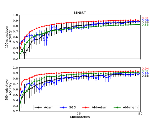
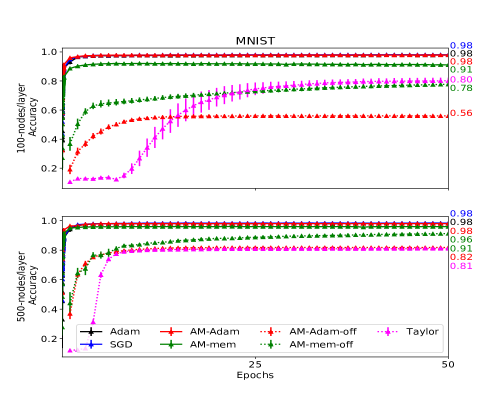
Figure 1: MNIST (fully-connected nets, 2 layers): online methods, first epoch; 50 mini-batches, 200 samples each.

Figure 2: MNIST (fully-connected nets, 2 layers): online vs. offline methods vs. Taylor’s ADMM, 50 epochs.

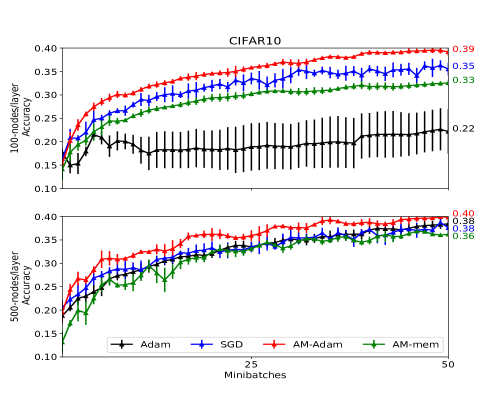
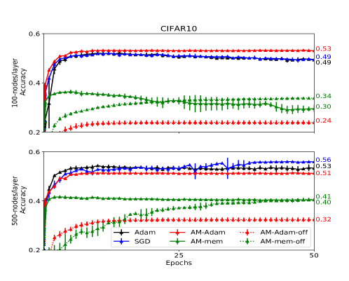
Figure 3: CIFAR10 (fully-connected nets): online methods, 1st epoch. 2 hidden layers with 100 (top) and 500 (bottom) units each; 250 mini-batches, 200 samples each.

Figure 4: CIFAR10 (fully-connected networks): online vs. offline, 50 epochs. Similar experiments to Figure 2.

4 Experiments

We compare on several datasets (MNIST, CIFAR10, HIGGS) our online alternating minimization algorithms, AM-mem and AM-Adam (using mini-batches instead of single samples at each time point), against backrop-based online methods, SGD and Adam (Kingma & Ba, 2014), as well as against the offline auxiliary-variable ADMM method of (Taylor et al., 2016), using code provided by the authors, and against the two offline versions of our methods, AM-Adam-off and AM-mem-off, which simply treat the training dataset as a single minibatch, i.e. one AM iteration is equivalent to one epoch over the training dataset. All our algorithms were implemented in PyTorch (Paszke et al., 2017); we also used PyTorch implementation of SGD and Adam. Hyperparameters used for each method were optimized by grid search on a validation subset of training data. Most results were averaged over at least 5 different weight initializations.

Note that most of the prior auxiliary-variable methods were evaluated only on fully-connected networks (Carreira-Perpiñán & Wang, 2014; Taylor et al., 2016; Zhang et al., 2016; Zhang & Brand, 2017; Zeng et al., 2018; Askari et al., 2018), while we also experiment with RNNs and CNNs, as well as with discrete (nondifferentiable) networks.

Fully-connected nets: MNIST, CIFAR10, HIGGS. We experiment with fully-connected networks on the standard MNIST (LeCun, 1998) dataset, consisting of $28\times 28$ gray-scale images of hand-drawn digits, with 50K samples, and a test set of 10K samples. We evaluate two different 2-hidden-layer architectures, with equal hidden layer sizes of 100 and 500, and ReLU activations. Figure 2 zooms in on the performance of the online methods, AM-Adam, AM-mem, SGD and Adam, over 50 minibatches of size 200 each. We observe that, on both architectures, AM-Adam is comparable to (in early stages, even slightly better than) SGD and Adam, while AM-mem is comparable with them on the larger architecture, and falls between SGD and Adam on the smaller one. Next, Figure 2 continues to 50 epochs, now including the offline methods (which require at least 1 epoch over the full dataset, by definition). Our AM-Adam method matches SGD and Adam, reaching 0.98 accuracy. Our second method, AM-mem only yields 0.91 and 0.96 on the 100-node and 500-node networks, respectively. All offline methods are significantly outperformed by the online ones; e.g., Taylor’s ADMM learns very slowly until about 10 epochs, being greatly outperformed even by our offline versions, but later catches up with offline AM-mem on the 100-node network; it is still inferior to all other methods on the 500-node architecture.

Figures 4 and 4 show similar results for the same experiment setting, on the CIFAR10 dataset (5000 training and 10000 test samples). Again, our AM-Adam performs slightly better than SGD and Adam on the first 50 minibatches (same size 200 as before), and even on 50 epochs for the 1-100 architecture, reaching 0.53 vs 0.49 accuracy of SGD and Adam, but falls a bit behind on the larger 1-500 architecture with 0.51 vs 0.53 and 0.56, respectively. Our second algorithm, AM-mem, is clearly dominated by all the three methods above. Also, we ran the two offline AM versions, which were again greatly outperformed by the online methods. In the remaining experiments, we focus on our best-performing method, online AM-Adam.

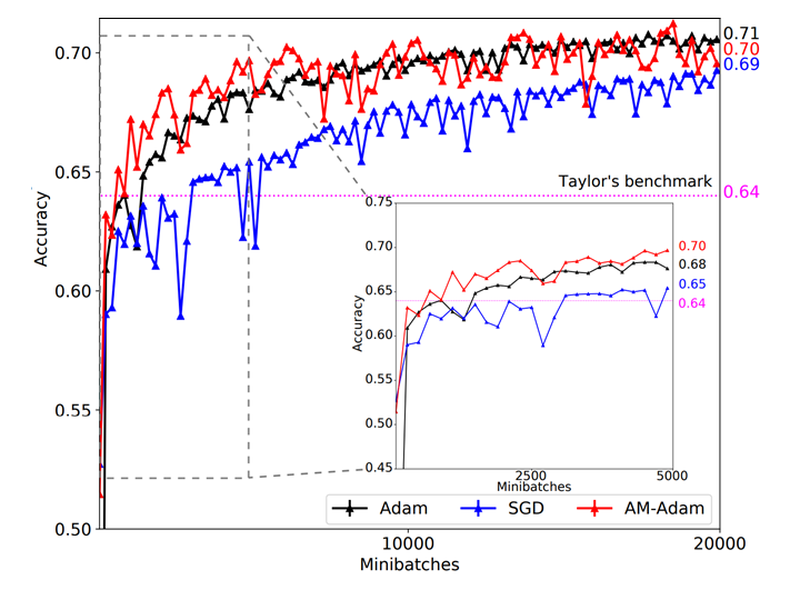
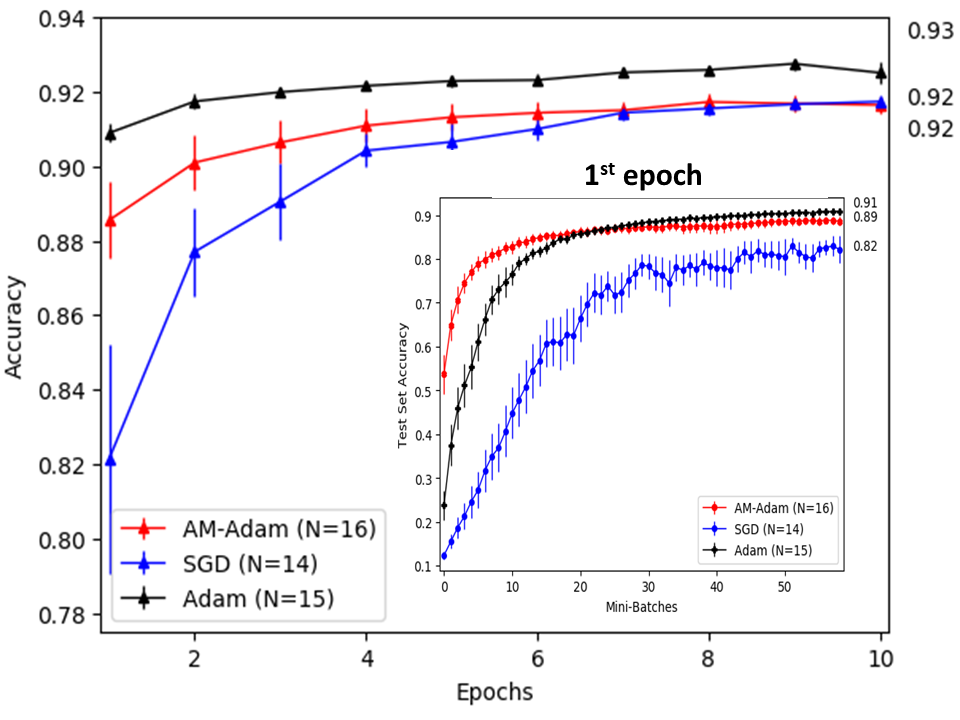
Figure 5: HIGGS dataset.

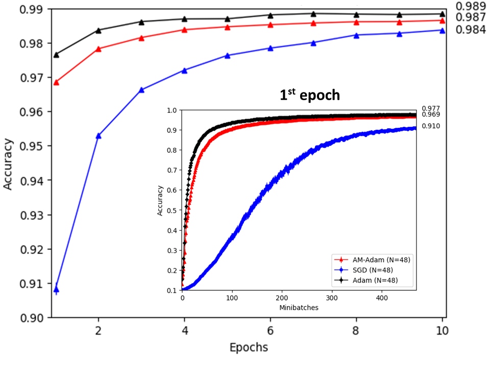
Figure 6: RNN-15, Sequential MNIST.

Figure 7: CNN: LeNet5, MNIST.

HIGGS, fully-connected, 1-300 ReLU network. In Figure 7, we compare our online AM-Adam approach against SGD, Adam and the offline ADMM method of Taylor, on a very large HIGGS dataset, containing 10,500,000 training samples (28 features each) and 500,000 test samples. Each datapoint is labeled as either a signal process producing a Higgs boson or a background process which does not. We use the same architecture (a single-hidden layer network with ReLU activations and 300 hidden nodes) as in (Taylor et al., 2016), and the same training/test data sets. For all online methods, we use minibatches of size 200, so one epoch over the 10.5M samples equals 52,500 iterations.

While Taylor’s method was reported to achieve 0.64 accuracy on the whole dataset (using data parallelization on 7200 cores to handle the whole dataset as a batch) (Taylor et al., 2016), the online methods achieve the same accuracy much faster (less than 1000 iterations/200K samples for our AM-Adam, and less than 2000 iterations for SGD and Adam; within only 20,000 iterations (less than a half of training samples), AM-Adam, SGD and Adam 0.70, 0.69 and 0.71, respectively, and continue to improve slowly, reaching after one epoch, 0.71, 0,71 and 0.72, respectively. (Our AM-mem version quickly reached 0.6 together with AM-Adam, but then slowed down, reaching only 0.61 on the 1st epoch).

In summary, on HIGGS dataset, AM-Adam, SGD and Adam clearly outperform Taylor’s offline ADMM, while using less than a half of the 1st epoch, and quickly reaching Taylor’s 0.64 accuracy benchmark after observing only a tiny fraction (less than 0.01%) of the 10.5M dataset. Both Adam and AM-Adam perform very closely, both outperforming SGD.

RNN on MNIST. Next, we evaluate our method on Sequential MNIST (Le et al., 2015), where each image is vectorized and fed to the RNN as a sequence of $T=784$ pixels. We use the standard Elman RNN architecture with $tanh$ activations among hidden states and ReLU applied to the output sequence before making a prediction (we use larger minibatches of 1024 samples to reduce training time). AM-Adam was adapted to work on such RNN architecture (see Appendix for details). Figure 7 shows the results using $d=15$ hidden units (see Appendix for $d=50$), averaged over N weight initializations, for 10 epochs, with a zoom-in on the first epoch inset. AM-Adam performs similarly to Adam in the 1st epoch, and outperforms SGD up to epoch 6, matching SGD’s performance afterwards.

CNN (LeNet-5), MNIST. Next, we experiment with CNNs, using LeNet-5 (LeCun et al., 1998) on MNIST (Figure 7). Similarly to RNN result, AM-Adam clearly outperforms SGD, while being somewhat outperformed by Adam.

Binary nets (nondifferentiable activations), MNIST. Finally, to investigate the ability of our method to handle non-differentiable networks, we consider an architecture originally investigated in (Lee et al., 2015) to evaluate another type of auxiliary-variable approach, called Difference Target Propagation (DTP). The model is a 2-hidden layer fully-connected network (784-500-500-10), whose first hidden layer uses the non-differentiable $sign$ transfer function (while the second hidden layer uses $\tanh$). Target propagation approaches were motivated by the goal of finding more biologically plausible mechanisms for credit assignment in the brain’s neural networks as compared to standard backprop, which, among multiple other biologically-implausible aspects, does not model the neuronal activation propagation explicitly, and does not handle non-differentiable binary activations (spikes) (Lee et al., 2015; Bartunov et al., 2018).

Figure 8: Binary net, MNIST.

In (Lee et al., 2015), DTP was applied to the above discrete network, and compared to a backprop-based straight-through estimator (STE), which simply ignores the derivative of the step function (which is 0 or infinite) in the back-propagation phase. While DTP took about 200 epochs to reach 0.2 error, matching the STE performance (Figure 3 in (Lee et al., 2015)), our AM-Adam with binary activations reaches the same error in less than 20 epochs (Figure 8).

5 Conclusions

We proposed a novel online alternating-minimization approach for neural network training; it builds upon previously proposed offline methods that break the nested objective into easier-to-solve local subproblems via inserting auxiliary variables corresponding to activations in each layer. Such methods avoid gradient chain computation and potential issues associated with it, including vanishing gradients, lack of cross-layer parallelization, and difficulties handling non-differentiable nonlinearities. However, unlike prior art, our approach is online (mini-batch), and thus can handle arbitrarily large datasets and continual learning settings. We proposed two variants, AM-mem and AM-Adam, and found that AM-Adam works better. Also, AM-Adam greatly outperforms offline methods on several datasets and architectures; when compared to state-of-the-art backprop methods such as (standard) SGD and Adam, AM-Adam typically matches their performance over multiple epochs, and may even learn somewhat faster initially, in small-data regimes. AM-Adam also converged faster than another related method, difference target propagation, on a discrete (non-differentiable) network. Finally, to the best of our knowledge, we are the first to provide theoretical guarantees for a wide class of online alternating minimization approaches including ours.

Supplementary Material

Appendix A Proofs

Proof of Theorem 3.2 relies on Theorem 3.1, which in turn relies on Theorem A.1 and Lemma A.1, both of which are stated below. Proofs of the lemma and theorems follow in the subsequent subsections.

The next result is a standard result from convex optimization (Theorem 2.1.14 in (Nesterov, 2014)) and is used in the proof of Theorem A.1 below.

Next, we introduce the population gradient AM operator, $\mathcal{G}_{i}(\boldsymbol{\theta}_{1},\boldsymbol{\theta}_{2},\dots,\boldsymbol{\theta}_{K}$), where $i=1,2,\dots,K$, defined as

$$\mathcal{G}_{i}(\boldsymbol{\theta}_{1},\boldsymbol{\theta}_{2},\dots,\boldsymbol{\theta}_{K})\coloneqq\boldsymbol{\theta}_{i}+\eta\nabla_{i}f(\boldsymbol{\theta}_{1},\boldsymbol{\theta}_{2},\dots,\boldsymbol{\theta}_{K}),$$

where $\eta$ is the step size.

Lemma A.1.

For any $d=1,2,\dots,K$, the gradient operator $\mathcal{G}_{d}(\boldsymbol{\theta}_{1}^{*},\boldsymbol{\theta}_{2}^{*},\dots,\boldsymbol{\theta}_{d-1}^{*},\boldsymbol{\theta}_{d},\boldsymbol{\theta}_{d+1}^{*},\dots,\boldsymbol{\theta}_{K-1}^{*},\boldsymbol{\theta}_{K}^{*})$ under Assumption 3.1 (strong concavity) and Assumption 3.2 (smoothness) with constant step size choice $0<\eta\leq\frac{2}{\mu_{d}+\lambda_{d}}$ is contractive, i.e.

$$\|\mathcal{G}_{d}(\boldsymbol{\theta}_{1}^{*},\dots,\boldsymbol{\theta}_{d-1}^{*},\boldsymbol{\theta}_{d},\boldsymbol{\theta}_{d+1}^{*},\dots,\boldsymbol{\theta}_{K}^{*})-\boldsymbol{\theta}_{d}^{*}\|_{2}\leq\left(1-\frac{2\eta\mu_{d}\lambda_{d}}{\mu_{d}+\lambda_{d}}\right)\|\boldsymbol{\theta}_{d}-\boldsymbol{\theta}^{*}_{d}\|_{2}$$ (11)

for all $\boldsymbol{\theta}_{d}\in B_{2}(r_{d},\boldsymbol{\theta}_{d}^{*})$.

The next theorem also holds for any $d$ from $1$ to $K$. Let $r_{1},\dots,r_{d-1},r_{d+1},\dots,r_{K}>0$ and $\boldsymbol{\theta}_{1}\in B_{2}(r_{1},\boldsymbol{\theta}_{1}^{*}),\dots,\boldsymbol{\theta}_{d-1}\in B_{2}(r_{d-1},\boldsymbol{\theta}_{d-1}^{*}),\boldsymbol{\theta}_{d+1}\in B_{2}(r_{d+1},\boldsymbol{\theta}_{d+1}^{*}),\dots,\boldsymbol{\theta}_{K}\in B_{2}(r_{k},\boldsymbol{\theta}_{K}^{*})$.

Theorem A.1.

For some radius $r_{d}>0$ and a triplet $(\gamma_{d},\lambda_{d},\mu_{d})$ such that $0\leq\gamma_{d}<\lambda_{d}\leq\mu_{d}$, suppose that the function $L(\boldsymbol{\theta}_{1}^{*},\boldsymbol{\theta}_{2}^{*},\dots,\boldsymbol{\theta}_{d-1}^{*},\boldsymbol{\theta}_{d},\boldsymbol{\theta}_{d+1}^{*},\dots,\boldsymbol{\theta}_{K-1}^{*},\boldsymbol{\theta}_{K}^{*})$ is $\lambda_{d}$-strongly concave (Assumption 3.1) and $\mu_{d}$-smooth (Assumption 3.2), and that the GS ($\gamma_{d}$) condition of Assumption 3.3 holds. Then the population gradient AM operator $\mathcal{G}_{d}(\boldsymbol{\theta}_{1},\boldsymbol{\theta}_{2},\dots,\boldsymbol{\theta}_{K})$ with step $\eta$ such that $0<\eta\leq\min_{i=1,2,\dots,K}\frac{2}{\mu_{i}+\lambda_{i}}$ is contractive over a ball $B_{2}(r_{d},\boldsymbol{\theta}_{d}^{*})$, i.e.

$$\|\mathcal{G}_{d}(\boldsymbol{\theta}_{1},\boldsymbol{\theta}_{2},\dots,\boldsymbol{\theta}_{K})-\boldsymbol{\theta}_{d}^{*}\|_{2}\leq(1-\xi\eta)\|\boldsymbol{\theta}_{d}-\boldsymbol{\theta}_{d}^{*}\|_{2}+\eta\gamma\sum_{\begin{subarray}{c}i=1\\ i\neq d\end{subarray}}^{K}\|\boldsymbol{\theta}_{i}-\boldsymbol{\theta}_{i}^{*}\|_{2}$$ (12)

where $\gamma\coloneqq\max_{i=1,2,\dots,K}\gamma_{i}$, and $\xi\coloneqq\min_{i=1,2,\dots,K}\frac{2\mu_{i}\lambda_{i}}{\mu_{i}+\lambda_{i}}$.

A.1 Proof of Theorem A.1

$$\|\mathcal{G}_{d}(\boldsymbol{\theta}_{1},\boldsymbol{\theta}_{2},\dots,\boldsymbol{\theta}_{K})-\boldsymbol{\theta}_{d}^{*}\|_{2}=\|\boldsymbol{\theta}_{d}+\eta\nabla_{d}L(\boldsymbol{\theta}_{1},\boldsymbol{\theta}_{2}\dots,\boldsymbol{\theta}_{K})-\boldsymbol{\theta}_{d}^{*}\|_{2}$$

by the triangle inequality we further get

$$\leq\|\boldsymbol{\theta}_{d}+\eta\nabla_{d}L(\boldsymbol{\theta}_{1}^{*},\dots,\boldsymbol{\theta}_{d-1}^{*},\boldsymbol{\theta}_{d},\boldsymbol{\theta}_{d+1}^{*},\dots,\boldsymbol{\theta}_{K}^{*})-\boldsymbol{\theta}_{d}^{*}\|_{2}$$

$$+\eta\|\nabla_{d}L(\boldsymbol{\theta}_{1},\dots,\boldsymbol{\theta}_{d},\dots,\boldsymbol{\theta}_{K})$$

$$-\nabla_{d}L(\boldsymbol{\theta}_{1}^{*},\dots,\boldsymbol{\theta}_{d-1}^{*},\boldsymbol{\theta}_{d},\boldsymbol{\theta}_{d+1}^{*},\dots,\boldsymbol{\theta}_{K}^{*})\|_{2}$$

by the contractivity of $$T$$ from Equation 11 from Lemma A.1 and GS condition

$$\leq\left(1-\frac{2\eta\mu_{d}\lambda_{d}}{\mu_{d}+\lambda_{d}}\right)\|\theta_{d}-\theta_{d}^{*}\|_{2}+\eta\gamma_{d}\sum_{\begin{subarray}{c}i=1\\ i\neq d\end{subarray}}^{K}\|\theta_{i}-\theta_{i}^{*}\|_{2}.$$

A.2 Proof of Theorem 3.1

Let $\boldsymbol{\theta}_{d}^{t+1}=\Pi_{d}(\boldsymbol{\tilde{\theta}}_{d}^{t+1})$, where $\boldsymbol{\tilde{\theta}}_{d}^{t+1}\coloneqq\boldsymbol{\theta}^{t}_{d}+\eta^{t}\nabla_{d}L^{1}(\boldsymbol{\theta}_{1}^{t+1},\boldsymbol{\theta}_{2}^{t+1},\dots,\boldsymbol{\theta}_{d-1}^{t+1},\boldsymbol{\theta}_{d}^{t},\boldsymbol{\theta}_{d+1}^{t},\dots,\boldsymbol{\theta}_{K}^{t})$ ($\nabla_{d}L^{1}$ is the gradient computed with respect to a single data sample) is the update vector prior to the projection onto a ball $B_{2}(\frac{r_{d}}{2},\boldsymbol{\theta}_{d}^{0})$. Let $\boldsymbol{\Delta}^{t+1}_{d}\coloneqq\boldsymbol{\theta}_{d}^{t+1}-\boldsymbol{\theta}_{d}^{*}$ and $\boldsymbol{\tilde{\Delta}}_{d}^{t+1}\coloneqq\boldsymbol{\tilde{\theta}}_{d}^{t+1}-\boldsymbol{\theta}_{d}^{*}$. Thus

$$\|\boldsymbol{\Delta}^{t+1}_{d}\|_{2}^{2}-\|\boldsymbol{\Delta}^{t}_{d}\|_{2}^{2} \leq \|\boldsymbol{\tilde{\Delta}}^{t+1}_{d}\|_{2}^{2}-\|\boldsymbol{\Delta}^{t}_{d}\|_{2}^{2}$$

$$= \|\boldsymbol{\tilde{\theta}}^{t+1}_{d}-\boldsymbol{\theta}_{d}^{*}\|-\|\boldsymbol{\theta}_{d}^{t}-\boldsymbol{\theta}_{d}^{*}\|$$

$$= \left<\boldsymbol{\tilde{\theta}}_{d}^{t+1}-\boldsymbol{\theta}_{d}^{t},\boldsymbol{\tilde{\theta}}_{d}^{t+1}+\boldsymbol{\theta}_{d}^{t}-2\boldsymbol{\theta}_{d}^{*}\right>.$$

Let $\boldsymbol{\hat{W}}_{d}^{t}\coloneqq\nabla_{d}L^{1}(\boldsymbol{\theta}_{1}^{t+1},\boldsymbol{\theta}_{2}^{t+1},\dots,\boldsymbol{\theta}_{d-1}^{t+1},\boldsymbol{\theta}_{d}^{t},\boldsymbol{\theta}_{d+1}^{t},\dots,\boldsymbol{\theta}_{K}^{t})$. Then we have that $\boldsymbol{\tilde{\theta}}_{d}^{t+1}-\boldsymbol{\theta}_{d}^{t}=\eta^{t}\boldsymbol{\hat{W}}_{d}^{t}$. We combine it with Equation A.2 and obtain:

$$\|\boldsymbol{\Delta}^{t+1}_{d}\|_{2}^{2}-\|\boldsymbol{\Delta}^{t}_{d}\|_{2}^{2}$$

$$\leq \left<\eta^{t}\boldsymbol{\hat{W}}_{d}^{t},\eta^{t}\boldsymbol{\hat{W}}_{d}^{t}+2(\boldsymbol{\theta}_{d}^{t}-\boldsymbol{\theta}_{d}^{*})\right>$$

$$= (\eta^{t})^{2}(\boldsymbol{\hat{W}}_{d}^{t})^{\top}\boldsymbol{\hat{W}}_{d}^{t}+2\eta^{t}(\boldsymbol{\hat{W}}_{d}^{t})^{\top}(\boldsymbol{\theta}_{d}^{t}-\boldsymbol{\theta}_{d}^{*})$$

$$= (\eta^{t})^{2}\|\boldsymbol{\hat{W}}_{d}^{t}\|_{2}^{2}+2\eta^{t}\left<\boldsymbol{\hat{W}}_{d}^{t},\boldsymbol{\Delta}^{t}_{d}\right>.$$

Let $\boldsymbol{W}_{d}^{t}\coloneqq\nabla_{d}L(\boldsymbol{\theta}_{1}^{t+1},\boldsymbol{\theta}_{2}^{t+1},\dots,\boldsymbol{\theta}_{d-1}^{t+1},\boldsymbol{\theta}_{d}^{t},\boldsymbol{\theta}_{d+1}^{t},\dots,\boldsymbol{\theta}_{K}^{t})$. Recall that $\mathbb{E}[\boldsymbol{\hat{W}}_{d}^{t}]=\boldsymbol{W}_{d}^{t}$. By the properties of martingales, i.e. iterated expectations and tower property:

$$\mathbb{E}[\|\boldsymbol{\Delta}^{t+1}_{d}\|_{2}^{2}] \leq \mathbb{E}[\|\boldsymbol{\Delta}^{t}_{d}\|_{2}^{2}]+(\eta^{t})^{2}\mathbb{E}[\|\boldsymbol{\hat{W}}_{d}^{t}\|_{2}^{2}]+2\eta^{t}\mathbb{E}[\left<\boldsymbol{W}_{d}^{t},\boldsymbol{\Delta}^{t}_{d}\right>]$$ (13)

Let $\boldsymbol{W}_{d}^{*}\coloneqq\nabla_{d}L(\boldsymbol{\theta}_{1}^{*},\boldsymbol{\theta}_{2}^{*},\dots,\boldsymbol{\theta}_{K}^{*})$. By self-consistency, i.e. $\boldsymbol{\theta}_{d}^{*}=\arg\max_{\boldsymbol{\theta}_{d}\in\Omega_{d}}L(\boldsymbol{\theta}_{1}^{*},\dots,\boldsymbol{\theta}_{d-1}^{*},\boldsymbol{\theta}_{d},\boldsymbol{\theta}_{d+1}^{*},\dots,\boldsymbol{\theta}_{K}^{*})$ and convexity of $\Omega_{d}$ we have that

$$\left<\boldsymbol{W}_{d}^{*},\boldsymbol{\Delta}^{t}_{d}\right>=\left<\nabla_{d}L(\boldsymbol{\theta}_{1}^{*},\boldsymbol{\theta}_{2}^{*},\dots,\boldsymbol{\theta}_{K}^{*}),\boldsymbol{\Delta}^{t}_{d}\right>\leq 0.$$

Combining this with Equation 13 we have

$$\mathbb{E}[\|\boldsymbol{\Delta}^{t+1}_{d}\|_{2}^{2}] \leq \mathbb{E}[\|\boldsymbol{\Delta}^{t}_{d}\|_{2}^{2}]+(\eta^{t})^{2}\mathbb{E}[\|\boldsymbol{\hat{W}}_{d}^{t}\|_{2}^{2}]+2\eta^{t}\mathbb{E}[\left<\boldsymbol{W}_{d}^{t}-\boldsymbol{W}_{d}^{*},\boldsymbol{\Delta}^{t}_{d}\right>].$$

Define $\mathcal{G}^{t}_{d}\coloneqq\boldsymbol{\theta}_{d}^{t}+\eta^{t}\boldsymbol{W}^{t}_{d}$ and $\mathcal{G}_{d}^{t*}\coloneqq\boldsymbol{\theta}_{d}^{*}+\eta^{t}\boldsymbol{W}_{d}^{*}$. Thus

$$\eta^{t}\left<\boldsymbol{W}_{d}^{t}-\boldsymbol{W}_{d}^{*},\boldsymbol{\Delta}^{t}_{d}\right>$$

$$= \left<\mathcal{G}_{d}^{t}-\mathcal{G}_{d}^{t*}-(\boldsymbol{\theta}^{t}_{d}-\boldsymbol{\theta}_{d}^{*}),\boldsymbol{\theta}^{t}_{d}-\boldsymbol{\theta}_{d}^{*}\right>$$

$$= \left<\mathcal{G}_{d}^{t}-\mathcal{G}_{d}^{t*},\boldsymbol{\theta}^{t}_{d}-\boldsymbol{\theta}_{d}^{*}\right>-\|\boldsymbol{\theta}^{t}_{d}-\boldsymbol{\theta}_{d}^{*}\|_{2}^{2}$$

by the fact that $$\mathcal{G}_{d}^{t*}=\boldsymbol{\theta}_{d}^{*}+\eta^{t}\boldsymbol{W}_{d}^{*}=\boldsymbol{\theta}_{d}^{*} \boldsymbol{W}_{d}^{*}=0$$ (since ):

$$= \left<\mathcal{G}_{d}^{t}-\boldsymbol{\theta}_{d}^{*},\boldsymbol{\theta}^{t}_{d}-\boldsymbol{\theta}_{d}^{*}\right>-\|\boldsymbol{\theta}^{t}_{d}-\boldsymbol{\theta}_{d}^{*}\|_{2}^{2}$$

by the contractivity of $$\mathcal{G}^{t}$$ from Theorem A.1:

$$\leq \left\{(1-\eta^{t}\xi)\|\boldsymbol{\theta}_{d}^{t}-\boldsymbol{\theta}_{d}^{*}\|+\eta^{t}\gamma\left(\sum_{i=1}^{d-1}\|\boldsymbol{\theta}_{i}^{t+1}-\boldsymbol{\theta}_{i}^{*}\|_{2}\right.\right.\left.\left.+\sum_{i=d+1}^{K}\|\boldsymbol{\theta}_{i}^{t}-\boldsymbol{\theta}_{i}^{*}\|_{2}\right)\right\}\|\boldsymbol{\theta}^{t}_{d}-\boldsymbol{\theta}_{d}^{*}\|_{2}-\|\boldsymbol{\theta}^{t}_{d}-\boldsymbol{\theta}_{d}^{*}\|_{2}^{2}$$

$$\leq \left\{(1-\eta^{t}\xi)\|\boldsymbol{\Delta}_{d}^{t}\|_{2}+\eta^{t}\gamma\left(\sum_{i=1}^{d-1}\|\boldsymbol{\Delta}_{i}^{t+1}\|_{2}+\sum_{i=d+1}^{K}\|\boldsymbol{\Delta}_{i}^{t}\|_{2}\right)\right\}\cdot\|\boldsymbol{\Delta}^{t}_{d}\|_{2}-\|\boldsymbol{\Delta}^{t}_{d}\|_{2}^{2}$$

Combining this result with Equation A.2 gives

$$\mathbb{E}[\|\boldsymbol{\Delta}^{t+1}_{d}\|_{2}^{2}] \leq \mathbb{E}[\|\boldsymbol{\Delta}^{t}_{d}\|_{2}^{2}]+(\eta^{t})^{2}\mathbb{E}[\|\boldsymbol{\hat{W}}_{d}^{t}\|_{2}^{2}]+2\mathbb{E}\left[\left\{(1-\eta^{t}\xi)\|\boldsymbol{\Delta}_{d}^{t}\|_{2}+\eta^{t}\gamma\left(\sum_{i=1}^{d-1}\|\boldsymbol{\Delta}_{i}^{t+1}\|_{2}+\sum_{i=d+1}^{K}\|\boldsymbol{\Delta}_{i}^{t}\|_{2}\right)\right\}\right.$$

$$\left.\cdot\|\boldsymbol{\Delta}^{t}_{d}\|_{2}-\|\boldsymbol{\Delta}^{t}_{d}\|_{2}^{2}\right]$$

$$\leq \mathbb{E}[\|\boldsymbol{\Delta}^{t}_{d}\|_{2}^{2}]+(\eta^{t})^{2}\sigma_{d}^{2}+2\mathbb{E}\left[\left\{(1-\eta^{t}\xi)\|\boldsymbol{\Delta}_{d}^{t}\|_{2}+\eta^{t}\gamma\left(\sum_{i=1}^{d-1}\|\boldsymbol{\Delta}_{i}^{t+1}\|_{2}+\sum_{i=d+1}^{K}\|\boldsymbol{\Delta}_{i}^{t}\|_{2}\right)\right\}\right.$$

$$\left.\cdot\|\boldsymbol{\Delta}^{t}_{d}\|_{2}-\|\boldsymbol{\Delta}^{t}_{d}\|_{2}^{2}\right],\>\>\>\text{where}$$

$\sigma_{d}^{2}=\sup_{\begin{subarray}{c}\boldsymbol{\theta}_{1}\in B_{2}(r_{1},\boldsymbol{\theta}_{1}^{*})\\ \dots\\ \boldsymbol{\theta}_{K}\in B_{2}(r_{K},\boldsymbol{\theta}_{K}^{*})\end{subarray}}\mathbb{E}[\|\nabla_{d}L^{1}(\boldsymbol{\theta}_{1},\boldsymbol{\theta}_{2},\dots,\boldsymbol{\theta}_{K})\|_{2}^{2}]$.

After re-arranging the terms we obtain

$$\mathbb{E}[\|\boldsymbol{\Delta}^{t+1}_{d}\|_{2}^{2}]\leq(\eta^{t})^{2}\sigma_{d}^{2}+(1-2\eta^{t}\xi)\mathbb{E}[\|\boldsymbol{\Delta}^{t}_{d}\|_{2}^{2}]+2\eta^{t}\gamma\mathbb{E}\left[\left(\sum_{i=1}^{d-1}\|\boldsymbol{\Delta}_{i}^{t+1}\|_{2}+\sum_{i=d+1}^{K}\|\boldsymbol{\Delta}_{i}^{t}\|_{2}\right)\|\boldsymbol{\Delta}^{t}_{d}\|_{2}\right]$$

apply $$2ab\leq a^{2}+b^{2}$$

$$\leq (\eta^{t})^{2}\sigma_{d}^{2}+(1-2\eta^{t}\xi)\mathbb{E}[\|\boldsymbol{\Delta}^{t}_{d}\|_{2}^{2}]+\eta^{t}\gamma\mathbb{E}\left[\sum_{i=1}^{d-1}\left(\|\boldsymbol{\Delta}_{i}^{t+1}\|_{2}^{2}+\|\boldsymbol{\Delta}^{t}_{d}\|_{2}^{2}\right)\right]+\eta^{t}\gamma\mathbb{E}\left[\sum_{i=d+1}^{K}\left(\|\boldsymbol{\Delta}_{i}^{t}\|_{2}^{2}+\|\boldsymbol{\Delta}^{t}_{d}\|_{2}^{2}\right)\right]$$

$$= (\eta^{t})^{2}\sigma_{d}^{2}+\mathbb{E}[\|\boldsymbol{\Delta}^{t}_{d}\|_{2}^{2}]\cdot\left[1-2\eta^{t}\xi+\eta^{t}\gamma(K-1)\right]+\eta^{t}\gamma\mathbb{E}\left[\sum_{i=1}^{d-1}\|\boldsymbol{\Delta}_{i}^{t+1}\|_{2}^{2}\right]+\eta^{t}\gamma\mathbb{E}\left[\sum_{i=d+1}^{K}\|\boldsymbol{\Delta}_{i}^{t}\|_{2}^{2}\right]$$

We obtained

$$\mathbb{E}[\|\boldsymbol{\Delta}^{t+1}_{d}\|_{2}^{2}]\leq(\eta^{t})^{2}\sigma_{d}^{2}+[1-2\eta^{t}\xi+\eta^{t}\gamma(K-1)]\mathbb{E}[\|\boldsymbol{\Delta}^{t}_{d}\|_{2}^{2}]+\eta^{t}\gamma\mathbb{E}\left[\sum_{i=1}^{d-1}\|\boldsymbol{\Delta}_{i}^{t+1}\|_{2}^{2}\right]+\eta^{t}\gamma\mathbb{E}\left[\sum_{i=d+1}^{K}\|\boldsymbol{\Delta}_{i}^{t}\|_{2}^{2}\right]$$

we next re-group the terms as follows

$$\mathbb{E}[\|\boldsymbol{\Delta}^{t+1}_{d}\|_{2}^{2}]-\eta^{t}\gamma\mathbb{E}\left[\sum_{i=1}^{d-1}\|\boldsymbol{\Delta}_{i}^{t+1}\|_{2}^{2}\right]\leq[1-2\eta^{t}\xi+\eta^{t}\gamma(K-1)]\mathbb{E}[\|\boldsymbol{\Delta}^{t}_{d}\|_{2}^{2}]+\eta^{t}\gamma\mathbb{E}\left[\sum_{i=d+1}^{K}\|\boldsymbol{\Delta}_{i}^{t}\|_{2}^{2}\right]+(\eta^{t})^{2}\sigma_{d}^{2}$$

and then sum over $$d 1 K$$ from to

$$\mathbb{E}\left[\sum_{d=1}^{K}\|\boldsymbol{\Delta}^{t+1}_{d}\|_{2}^{2}\right]-\eta^{t}\gamma\mathbb{E}\left[\sum_{d=1}^{K}\sum_{i=1}^{d-1}\|\boldsymbol{\Delta}_{i}^{t+1}\|_{2}^{2}\right]$$

$$\leq [1-2\eta^{t}\xi+\eta^{t}\gamma(K-1)]\mathbb{E}\left[\sum_{d=1}^{K}\|\boldsymbol{\Delta}^{t}_{d}\|_{2}^{2}\right]+\eta^{t}\gamma\mathbb{E}\left[\sum_{d=1}^{K}\sum_{i=d+1}^{K}\|\boldsymbol{\Delta}_{i}^{t}\|_{2}^{2}\right]+(\eta^{t})^{2}\sum_{d=1}^{K}\sigma_{d}^{2}$$

Let $\sigma=\sqrt{\sum_{d=1}^{K}\sigma_{d}^{2}}$. Also, note that

$$\mathbb{E}\left[\sum_{d=1}^{K}\|\boldsymbol{\Delta}^{t+1}_{d}\|_{2}^{2}\right]-\eta^{t}\gamma(K-1)\mathbb{E}\left[\sum_{d=1}^{K}\|\boldsymbol{\Delta}_{d}^{t+1}\|_{2}^{2}\right]\leq\mathbb{E}\left[\sum_{d=1}^{K}\|\boldsymbol{\Delta}^{t+1}_{d}\|_{2}^{2}\right]-\eta^{t}\gamma\mathbb{E}\left[\sum_{d=1}^{K}\sum_{i=1}^{d-1}\|\boldsymbol{\Delta}_{i}^{t+1}\|_{2}^{2}\right]$$

and

$$[1-2\eta^{t}\xi+\eta^{t}\gamma(K-1)]\mathbb{E}\left[\sum_{d=1}^{K}\|\boldsymbol{\Delta}^{t}_{d}\|_{2}^{2}\right]+\eta^{t}\gamma\mathbb{E}\left[\sum_{d=1}^{K}\sum_{i=d+1}^{K}\|\boldsymbol{\Delta}_{i}^{t}\|_{2}^{2}\right]+(\eta^{t})^{2}\sigma^{2}$$

$$\leq [1-2\eta^{t}\xi+\eta^{t}\gamma(K-1)]\mathbb{E}\left[\sum_{d=1}^{K}\|\boldsymbol{\Delta}^{t}_{d}\|_{2}^{2}\right]+\eta^{t}\gamma(K-1)\mathbb{E}\left[\sum_{d=1}^{K}\|\Delta_{d}^{t}\|_{2}^{2}\right]+(\eta^{t})^{2}\sigma^{2}$$

Combining these two facts with our previous results yields:

$$[1-(K-1)\eta^{t}\gamma]\mathbb{E}\left[\sum_{d=1}^{K}\|\boldsymbol{\Delta}^{t+1}_{d}\|_{2}^{2}\right]$$

$$\leq [1-2\eta^{t}\xi+\eta^{t}\gamma(K-1)]\mathbb{E}\left[\sum_{d=1}^{K}\|\boldsymbol{\Delta}^{t}_{d}\|_{2}^{2}\right]+\eta^{t}\gamma(K-1)\mathbb{E}\left[\sum_{d=1}^{K}\|\boldsymbol{\Delta}_{d}^{t}\|_{2}^{2}\right]+(\eta^{t})^{2}\sigma^{2}$$

$$= [1-2\eta^{t}\xi+2\eta^{t}\gamma(K-1)]\mathbb{E}\left[\sum_{d=1}^{K}\|\boldsymbol{\Delta}^{t}_{d}\|_{2}^{2}\right]+(\eta^{t})^{2}\sigma^{2}$$

Thus:

$$\mathbb{E}\left[\sum_{d=1}^{K}\|\boldsymbol{\Delta}^{t+1}_{d}\|_{2}^{2}\right] \leq \frac{1-2\eta^{t}\xi+2\eta^{t}\gamma(K-1)}{1-(K-1)\eta^{t}\gamma}\mathbb{E}\left[\sum_{d=1}^{K}\|\boldsymbol{\Delta}^{t}_{d}\|_{2}^{2}\right]$$

$$+ \frac{(\eta^{t})^{2}}{1-(K-1)\eta^{t}\gamma}\sigma^{2}.$$

Since $\gamma<\frac{2\xi}{3(K-1)}$, $\frac{1-2\eta^{t}\xi+2\eta^{t}\gamma(K-1)}{1-(K-1)\eta^{t}\gamma}<1$.

A.3 Proof of Theorem 3.2

To obtain the final theorem we need to expand the recursion from Theorem 3.1. We obtained

$$\mathbb{E}\left[\sum_{d=1}^{K}\|\boldsymbol{\Delta}^{t+1}_{d}\|_{2}^{2}\right]$$

$$\leq\frac{1-2\eta^{t}[\xi-\gamma(K-1)]}{1-(K-1)\eta^{t}\gamma}\mathbb{E}\left[\sum_{d=1}^{K}\|\boldsymbol{\Delta}^{t}_{d}\|_{2}^{2}\right]+\frac{(\eta^{t})^{2}}{1-(K-1)\eta^{t}\gamma}\sigma^{2}$$

$$=\left(1-\frac{\eta^{t}[2\xi-3\gamma(K-1)]}{1-(K-1)\eta^{t}\gamma}\right)\mathbb{E}\left[\sum_{d=1}^{K}\|\boldsymbol{\Delta}^{t}_{d}\|_{2}^{2}\right]+\frac{(\eta^{t})^{2}}{1-(K-1)\eta^{t}\gamma}\sigma^{2}$$

Recall that we defined $q^{t}$ in Theorem 3.1 as

$$q^{t}=1-\frac{1-2\eta^{t}\xi+2\eta^{t}\gamma(K-1)}{1-(K-1)\eta^{t}\gamma}=\frac{\eta^{t}[2\xi-3\gamma(K-1)]}{1-(K-1)\eta^{t}\gamma}$$

and denote

$$\beta^{t}=\frac{(\eta^{t})^{2}}{1-(K-1)\eta^{t}\gamma}.$$

Thus we have

$$\mathbb{E}\left[\sum_{d=1}^{K}\|\boldsymbol{\Delta}^{t+1}_{d}\|_{2}^{2}\right]\leq(1-q^{t})\mathbb{E}\left[\sum_{d=1}^{K}\|\boldsymbol{\Delta}^{t}_{d}\|_{2}^{2}\right]+\beta^{t}\sigma^{2}$$

$$\leq (1-q^{t})\left\{(1-q^{t-1})\mathbb{E}\left[\sum_{d=1}^{K}\|\Delta^{t-1}_{d}\|_{2}^{2}\right]+\beta^{t-1}\sigma^{2}\right\}+\beta^{t}\sigma^{2}$$

$$= (1-q^{t})(1-q^{t-1})\mathbb{E}\left[\sum_{d=1}^{K}\|\boldsymbol{\Delta}^{t-1}_{d}\|_{2}^{2}\right]+(1-q^{t})\beta^{t-1}\sigma^{2}+\beta^{t}\sigma^{2}$$

$$\leq (1-q^{t})(1-q^{t-1})\left\{(1-q^{t-2})\mathbb{E}\left[\sum_{d=1}^{K}\|\boldsymbol{\Delta}^{t-2}_{d}\|_{2}^{2}\right]+\beta^{t-2}\sigma^{2}\right\}+(1-q^{t})\beta^{t-1}\sigma^{2}+\beta^{t}\sigma^{2}$$

$$= (1-q^{t})(1-q^{t-1})(1-q^{t-2})\mathbb{E}\left[\sum_{d=1}^{K}\|\boldsymbol{\Delta}^{t-2}_{d}\|_{2}^{2}\right]$$

$$+(1-q^{t})(1-q^{t-1})\beta^{t-2}\sigma^{2}+(1-q^{t})\beta^{t-1}\sigma^{2}+\beta^{t}\sigma^{2}$$

We end-up with the following

$$\mathbb{E}\left[\sum_{d=1}^{K}\|\boldsymbol{\Delta}^{t+1}_{d}\|_{2}^{2}\right] \leq \mathbb{E}\left[\sum_{d=1}^{K}\|\boldsymbol{\Delta}^{0}_{d}\|_{2}^{2}\right]\prod_{i=0}^{t}(1-q^{i})+\sigma^{2}\sum_{i=0}^{t-1}\beta^{i}\prod_{j=i+1}^{t}(1-q^{j})+\beta^{t}\sigma^{2}.$$

Set $q^{t}=\frac{\frac{3}{2}}{t+2}$ and

$$\eta^{t} = \frac{q^{t}}{2\xi-3\gamma(K-1)+q^{t}(K-1)\gamma}$$

$$= \frac{\frac{3}{2}}{[2\xi-3\gamma(K-1)](t+2)+\frac{3}{2}(K-1)\gamma}.$$

Denote $A=2\xi-3\gamma(K-1)$ and $B=\frac{3}{2}(K-1)\gamma$. Thus

$$\eta^{t}=\frac{\frac{3}{2}}{A(t+2)+B}$$

and

$$\beta^{t}=\frac{(\eta^{t})^{2}}{1-\frac{2}{3}B\eta^{t}}=\frac{\frac{9}{4}}{A(t+2)[A(t+2)+B]}.$$

$$\mathbb{E}\left[\sum_{d=1}^{K}\|\boldsymbol{\Delta}^{t+1}_{d}\|_{2}^{2}\right]$$

$$\leq \mathbb{E}\left[\sum_{d=1}^{K}\|\boldsymbol{\Delta}^{0}_{d}\|_{2}^{2}\right]\prod_{i=0}^{t}\left(1-\frac{\frac{3}{2}}{i+2}\right)+\sigma^{2}\sum_{i=0}^{t-1}\frac{\frac{9}{4}}{A(i+2)[A(i+2)+B]}\prod_{j=i+1}^{t}\left(1-\frac{\frac{3}{2}}{j+2}\right)$$

$$+\sigma^{2}\frac{\frac{9}{4}}{A(t+2)[A(t+2)+B]}$$

$$= \mathbb{E}\left[\sum_{d=1}^{K}\|\boldsymbol{\Delta}^{0}_{d}\|_{2}^{2}\right]\prod_{i=2}^{t+2}\left(1-\frac{\frac{3}{2}}{i}\right)+\sigma^{2}\sum_{i=2}^{t+1}\frac{\frac{9}{4}}{Ai[Ai+B]}\prod_{j=i+1}^{t+2}\left(1-\frac{\frac{3}{2}}{j}\right)+\sigma^{2}\frac{\frac{9}{4}}{A(t+2)[A(t+2)+B]}$$

Since $A>0$ and $B>0$ thus

$$\mathbb{E}\left[\sum_{d=1}^{K}\|\boldsymbol{\Delta}^{t+1}_{d}\|_{2}^{2}\right]$$

$$\leq \mathbb{E}\left[\sum_{d=1}^{K}\|\boldsymbol{\Delta}^{0}_{d}\|_{2}^{2}\right]\prod_{i=2}^{t+2}\left(1-\frac{\frac{3}{2}}{i}\right)+\sigma^{2}\sum_{i=2}^{t+1}\frac{\frac{9}{4}}{Ai[Ai+B]}\prod_{j=i+1}^{t+2}\left(1-\frac{\frac{3}{2}}{j}\right)+\sigma^{2}\frac{\frac{9}{4}}{A(t+2)[A(t+2)+B]}$$

$$\leq \mathbb{E}\left[\sum_{d=1}^{K}\|\boldsymbol{\Delta}^{0}_{d}\|_{2}^{2}\right]\prod_{i=2}^{t+2}\left(1-\frac{\frac{3}{2}}{i}\right)+\sigma^{2}\sum_{i=2}^{t+1}\frac{\frac{9}{4}}{(Ai)^{2}}\prod_{j=i+1}^{t+2}\left(1-\frac{\frac{3}{2}}{j}\right)+\sigma^{2}\frac{\frac{9}{4}}{[A(t+2)]^{2}}$$

We can next use the fact that for any $a\in(1,2)$:

$$\prod_{i=\tau+1}^{t+2}\left(1-\frac{a}{i}\right)\leq\left(\frac{\tau+1}{t+3}\right)^{a}.$$

The bound then becomes

$$\mathbb{E}\left[\sum_{d=1}^{K}\|\boldsymbol{\Delta}^{t+1}_{d}\|_{2}^{2}\right]$$

$$\leq \mathbb{E}\left[\sum_{d=1}^{K}\|\boldsymbol{\Delta}^{0}_{d}\|_{2}^{2}\right]\prod_{i=2}^{t+2}\left(1-\frac{\frac{3}{2}}{i}\right)+\sigma^{2}\sum_{i=2}^{t+1}\frac{\frac{9}{4}}{(Ai)^{2}}\prod_{j=i+1}^{t+2}\left(1-\frac{\frac{3}{2}}{j}\right)+\sigma^{2}\frac{\frac{9}{4}}{[A(t+2)]^{2}}$$

$$\leq \mathbb{E}\left[\sum_{d=1}^{K}\|\boldsymbol{\Delta}^{0}_{d}\|_{2}^{2}\right]\left(\frac{2}{t+3}\right)^{\frac{3}{2}}+\sigma^{2}\sum_{i=2}^{t+1}\frac{\frac{9}{4}}{(Ai)^{2}}\left(\frac{i+1}{t+3}\right)^{\frac{3}{2}}+\sigma^{2}\frac{\frac{9}{4}}{[A(t+2)]^{2}}$$

$$= \mathbb{E}\left[\sum_{d=1}^{K}\|\boldsymbol{\Delta}^{0}_{d}\|_{2}^{2}\right]\left(\frac{2}{t+3}\right)^{\frac{3}{2}}+\sigma^{2}\sum_{i=2}^{t+2}\frac{\frac{9}{4}}{(Ai)^{2}}\left(\frac{i+1}{t+3}\right)^{\frac{3}{2}}$$

Note that $(i+1)^{\frac{3}{2}}\leq 2i$ for $i=2,3,\dots$, thus

$$\mathbb{E}\left[\sum_{d=1}^{K}\|\boldsymbol{\Delta}^{t+1}_{d}\|_{2}^{2}\right]$$

$$\leq \mathbb{E}\left[\sum_{d=1}^{K}\|\boldsymbol{\Delta}^{0}_{d}\|_{2}^{2}\right]\left(\frac{2}{t+3}\right)^{\frac{3}{2}}+\sigma^{2}\frac{\frac{9}{4}}{A^{2}(t+3)^{\frac{3}{2}}}\sum_{i=2}^{t+2}\frac{(i+1)^{\frac{3}{2}}}{i^{2}}$$

$$\leq \mathbb{E}\left[\sum_{d=1}^{K}\|\boldsymbol{\Delta}^{0}_{d}\|_{2}^{2}\right]\left(\frac{2}{t+3}\right)^{\frac{3}{2}}+\sigma^{2}\frac{\frac{9}{2}}{A^{2}(t+3)^{\frac{3}{2}}}\sum_{i=2}^{t+2}\frac{1}{i^{\frac{1}{2}}}$$

finally note that $$\sum_{i=2}^{t+2}\frac{1}{i^{\frac{1}{2}}}\leq\int_{1}^{t+2}\frac{1}{x^{\frac{1}{2}}}dx\leq 2(t+3)^{\frac{1}{2}}$$. Thus

$$\leq \mathbb{E}\left[\sum_{d=1}^{K}\|\boldsymbol{\Delta}^{0}_{d}\|_{2}^{2}\right]\left(\frac{2}{t+3}\right)^{\frac{3}{2}}+\sigma^{2}\frac{9}{A^{2}(t+3)}$$

substituting $$A=2\xi-3\gamma(K-1)$$ gives

$$= \mathbb{E}\left[\sum_{d=1}^{K}\|\boldsymbol{\Delta}^{0}_{d}\|_{2}^{2}\right]\left(\frac{2}{t+3}\right)^{\frac{3}{2}}+\sigma^{2}\frac{9}{[2\xi-3\gamma(K-1)]^{2}(t+3)}$$

This leads us to the final theorem.

Appendix B CNNs experiments: details

We compare SGD, Adam, and AM-Adam on the LeNet-5(LeCun et al., 1998) architecture on both MNIST and Fashion-MNIST (Xiao et al., 2017) datasets.

Fashion-MNIST is a dataset of Zalando’s article images, consisting of a training set of 60,000 examples and a test set of 10,000 examples. Each example is a 28x28 grayscale image, associated with a label from 10 classes. We intend Fashion-MNIST to serve as a direct drop-in replacement for the original MNIST dataset for benchmarking machine learning algorithms. It shares the same image size and structure of training and testing splits.

We fix the batchsize to 128, and run a hyperparameter grid search for each algorithm and dataset using the following values: weight-learning rates of 2e-M for M=2,3,4,5; batch-wise mu-increments of 1e-2,1e-5, 1e-7; epoch-wise mu-multipliers of 1, 1,1; code learning-rates of 0.1, 1 (note: only weight learning rates are varied for SGD and Adam). SGD was allowed a standard epoch-wise learning rate decay of 0.9. AM-Adam used only one subproblem iteration (both codes and weights) for each minibatch, an initial $\mu$ value of 0.01, and a maximum $\mu$ value of 1.5. In total, six total grid searches were performed.

For each hyperparameter combination, each algorithm was run on at least 5 initializations, training for 10 epochs on 5/6 of the training dataset. The mean final accuracy on the validation set (the remaining 1/6 of the training dataset) was used to select the best hyperparameters.

Finally, each algorithm with its best hyperparameters on each dataset was used to re-train Lenet-5 with N intializations, this time evaluated on the test set. The mean performances are plotted in Figures 9 for MNIST (left) and Fashion-MNIST (right).

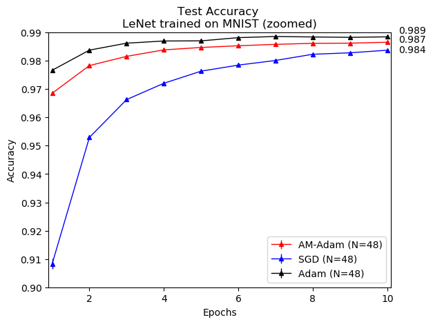
Figure 9: CNN using LeNet-5, MNIST(left) and Fashion-MNIST (right).

The winning hyperparameters for Fashion-MNIST are: Adam: LR=0.002 SGD: LR=0.02 AM: weight-LR= 0.002; code-LR= 1.0; batchwise $\mu$-increment=1e-5; epochwise $\mu$-multiplier=1.1

The winning hyperparameters for MNIST are: Adam: LR=0.002 SGD: LR=0.02 AM: weight-LR= 0.002; code-LR= 1.0; batchwise $\mu$-increment=1e-7; epochwise $\mu$-multiplier=1.1

Appendix C RNN experiments: details

C.1 Architecture and AM Adaptation

We also compare SGD, Adam, and AM-Adam on a standard Elman RNN architecture. That is a recurrent unit that, at time $t$, yields an output $z^{t}$ and hidden state $h^{t}$ based on a combination of input $x^{t}$ and the previous hidden state $h^{t-1}$, for $t=1,...,T$. The equations for the unit are:

$$h^{t} =\sigma\{\mathbf{U}x^{t}+\mathbf{W}h^{t-1}+\mathbf{b}\}$$ (14)

$$z^{t} =\mathbf{V}h^{t},$$ (15)

where $\mathbf{b}$ is a bias, $\sigma$ is a tanh activation function, and $\mathbf{U}\in\mathbb{R}^{d\times 1},\mathbf{W}\in\mathbb{R}^{d\times d},$ and $\mathbf{V}\in\mathbb{R}^{1\times d}$ are learnable parameter matrices that do not vary with $t$. Denote with $m$ the length of one sequence element, so $x^{t},z^{t}\in\mathbb{R}^{m}$. Then let $d$ be the number of hidden units, so $h^{t}\in\mathbb{R}^{d}$.

We train this architecture to classify MNIST digits where each image is vectorized and fed to the RNN as a sequence of $T=784$ pixels (termed "Sequential MNIST" in (Le et al., 2015)). Thus for each $t$, the input $x^{t}$ is a single pixel. A final matrix $\mathbf{C}$ is then used to classify the output sequence $z^{t}$ using the same multinomial loss function as before:

$$\sum_{n}\mathcal{L}(y_{n},ReLU(\mathbf{z}_{n}),\mathbf{C}),$$ (16)

where $\mathbf{z}_{n}=[z_{n}^{1},...,z_{n}^{784}]^{\text{T}}$ is the output sequence for the $n^{th}$ training sample, and $\mathbf{C}\in\mathbb{R}^{10\times 784}$. In summary, the prediction is made only after processing all 784 pixels.

To train this family of architectures using Alt-Min, we introduce two sets of auxiliary variables (codes). First, we introduce a code for each element of the sequence just before input to the activation function:

$$c^{t}=\mathbf{U}x^{t}+\mathbf{W}h^{t-1}+\mathbf{b}$$ (17)

where $c^{t}$ is the internal RNN code at time $t$. Using the "unfolded" interpretation of an RNN, we have introduced a code between each repeated "layer". Second, we treat the output sequence $\mathbf{z}$ as an auxiliary variable in order to break the gradient chain between the loss function and the recurrent unit.

C.2 Experiments

We compare SGD, Adam, and AM-Adam on the Elman RNN architecture with hidden sizes $d=15$ and $d=50$ on the Sequential MNIST dataset. We fix the batchsize to 1024, and run a hyperparameter grid search for each algorithm using the following values: weight-learning rates of 5e-M, for M=1,2,3,4,5 (all methods); weight sparsity = 0, 0.01, 0.1 (SGD and Adam); batch-wise mu-increment 1e-M for M=2,3,4; epoch-wise mu-multiplier for 1, 1.1, 1.25, 1.5; mu-max=1, 5. SGD was allowed a standard learning-rate-decay of 0.9. AM-Adam used an initial $\mu$ value of 0.01, and used 5 subproblem iterations for both code and weight optimization subproblems.

Note: in an offline hand-tuning search, we determined that weight-sparsity only hurt Alt-Min, so it was not included in official the grid search. Also note that a larger batchsize is used for the RNN experiments because of the relatively strong dependence of the training time on batchsize. This dependence is because for each minibatch, a series of loops though $t=1,...,784$ are required.

For each hyperparameter combination, each algorithm was run on at least 3 initializations, training for 10 epochs on 5/6 of the training dataset. The mean final accuracy on the validation set (the remaining 1/6 of the training dataset) was used to select the best hyperparameters.

Finally, each algorithm with its best hyperparameters on each dataset was used to re-train the Elman RNN with N intializations, this time evaluated on the test set.

The winning hyperparameters for d=15 are: Adam: learning rate = 0.005, L1=0; SGD: learning rate = 0.05, L1=0; AM-Adam: learning rate = 0.005, max-mu=1, mu-multiplier=1.1, mu-increment=0.01. Results are depicted in Figure 7.

The winning hyperparameters for d=50 are: Adam: learning rate = 0.005, L1=0.01; SGD: learning rate = 0.005, L1=0; AM-Adam: learning rate = 0.005, max-mu=1, mu-multiplier=1.0, mu-increment=0.0001. Results are depicted in Figure 10.

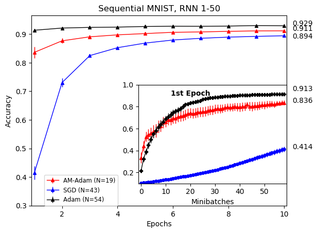
Figure 10: RNN-50, Sequential MNIST.

Appendix D Fully connected networks: details

Performance of the online (i.e., SGD, Adam, AM-Adam, AM-mem) and offline (i.e., AM-Adam-off, AM-mem-off, Taylor) methods are compared on the MNIST and CIFAR-10 datasets for two fully connected network architectures with two identical hidden layers of 100 and 500 units each. We also consider a different architecture with one hidden layer of 300 units for the larger HIGGS dataset. Optimal hyperparameters are reported below for each set of experiments.

D.1 MNIST Experiments

The standard MNIST training dataset is split into a reduced training set (first 50,000 samples) and a validation set (last 10,000 samples) for hyperparameter optimization. More specifically, an iterative bayesian optimization scheme is used to find the optimal learning rates (lr) maximizing classification accuracy on the validation set after 50 epochs of training. Rather than learning rates, for Taylor’s method we optimize the $\gamma_{\textrm{prod}}$ and ${\gamma_{\textrm{nonlin}}}$ parameters. The procedure is repeated for five different weight initializations and for both architectures considered. Table 1 reports hyperparameters yielding the highest accuracy among the 5 weight initializations.

Algorithm	Hidden units per layer	lr	$\gamma_{\textrm{prod}}$	$\gamma_{\textrm{nonlin}}$
Adam	100	0.0210
Adam	500	0.0005
SGD	100	0.2030
SGD	500	0.1497
AM-Adam	100	0.1973
AM-Adam	500	0.1171
AM-mem	100	0.1737
AM-mem	500	0.1376
AM-Adam-off	100	0.5003
AM-Adam-off	500	0.4834
AM-mem-off	100	0.4664
AM-mem-off	500	0.2503
Taylor	100		582.8	54.15
Taylor	500		444.2	111.7

Table 1: Optimal hyperparameters for fully connected networks on MNIST

D.2 CIFAR-10 Experiments

Similary to what done for the MNIST dataset, we split the standard CIFAR-10 training dataset into a reduced training set (first 40,000 samples) and a validation set (last 10,000 samples) used to evaluate accuracy for hyperparameter optimization. Table 2 reports hyperparameters for all the methods yielding the highest accuracy among the 5 weight initializations. Since not included in the original publication, we do not consider Taylor’s method on this dataset.

Algorithm	Hidden units per layer	lr
Adam	100	0.0029
Adam	500	0.0002
SGD	100	0.1500
SGD	500	0.1428
AM-Adam	100	0.1974
AM-Adam	500	0.1011
AM-mem	100	0.1746
AM-mem	500	0.1016
AM-Adam-off	100	0.5000
AM-Adam-off	500	0.4844
AM-mem-off	100	0.2343
AM-mem-off	500	0.2277

Table 2: Optimal hyperparameters for fully connected networks on CIFAR-10

D.3 HIGGS Experiments

For the Higgs experiment, we compare only our best performing AM-Adam online method to Adam and SGD. Also, due to the increased computational costs associated to this dataset, we consider only one weight initialization and replace the bayesian optimization scheme with a simpler grid search. Table 3 reports the hyperparameters yielding the highest accuracy.

Algorithm	Hidden units per layer	lr
Adam	300	0.001
SGD	300	0.050
AM-Adam	300	0.001

Table 3: Hyperparameters used for fully connected networks on HIGGS

D.4 Related Work: ProxProp

As we mentioned in the introduction, a closely related auxiliary methods, called ProxProp, was recently proposed in (Thomas Frerix, 2018). However, there are several importnant differences between ProxProp and our approach. ProxProp only analyzes and experimentally evaluates a batch version, only briefly mentioning in section 4.2.3 that theory is extendable to mini-batch setting, without explicit convergence rates/formal proofs/experiments. Also, an assumption on eigenvalues (from eq. 14 in (Thomas Frerix, 2018)) bounded away from zero is mentioned; however, in flat regions of optimization landscape (often found by solvers like SGD) this condition is not met, as most eigenvalues are close to zero (see, e.g. Chaudhari et al 2016). We believe that our assumptions are less restrictive from that perspective (and convergence in mini-batch setting is formally proven). Further differences include: (1) our formulation involves only one set of auxiliary variables/”codes” (linear z in ProxProp) rather than two (linear and nonlinear), reducing memory footprint (and potentially computing time); (2) ProxProp experiments are limited to batch mode, while we compare batch vs mini-batch vs SGD; (3) ProxProp processes both auxiliary variables and weights sequentially, layer by layer (we process auxiliary variables first, then weights in all layers independently/in parallel), which is important for ProxProp. (4) Finally, we also propose two different mini-batch methods, AM-SGD (closer to ProxProp) and AM-mem, which is very different from ProxProp as. it exploits surrogate objective method of online dictionary learning in (Mairal et al., 2009).

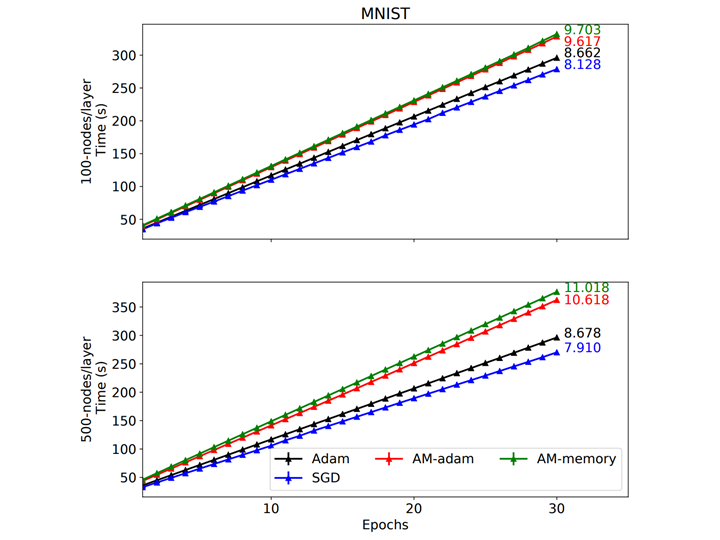
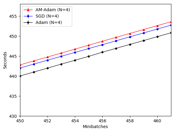
Figure 11: Runtimes on MNIST, fully-connected architecture

Figure 12: Runtimes on MNIST, LeNet5.

D.5 Computational Efficiency: Runtimes

Runtime results for AM-Adam were quite comparable in most experiments to those of Adam and SGD (see Figures 12 and 12). Runtimes of all methods grew linearly with mini-batches/epochs, and were similar to each other: e.g., for LeNet/MNIST (Figure 12), practically same slope was observed for all methods, and the runtimes were really close (e.g. 440, 442 and 443 seconds for 450 mini-batches for Adam, SGD and AM, respectively). On MNIST, using fully-connected networks (Figure 12), slight increase was observed in the slope of AM versus SGD and Adam, but the times were quite comparable: e.g., at 30 epochs, Adam took 8.7 seconds, while AM-SGD and AM-mem took 9.6 and 9.7 seconds, respectively. Note that we are comparing an implementation of AM which does not yet exploit parallelization; the latter is likely to provide a considerable speedup, similar to the one presented in (Carreira-Perpiñán & Wang, 2014).

References

• Askari et al. (2018) Askari, A., Negiar, G., Sambharya, R., and El Ghaoui, L. Lifted neural networks. arXiv:1805.01532 [cs.LG], 2018.
• Balakrishnan et al. (2017) Balakrishnan, S., Wainwright, M. J., and Yu, B. Statistical guarantees for the em algorithm: From population to sample-based analysis. Ann. Statist., 45(1):77–120, 02 2017. doi: 10.1214/16-AOS1435. URL https://doi.org/10.1214/16-AOS1435.
• Bartunov et al. (2018) Bartunov, S., Santoro, A., Richards, B., Marris, L., Hinton, G. E., and Lillicrap, T. Assessing the scalability of biologically-motivated deep learning algorithms and architectures. In Advances in Neural Information Processing Systems, pp. 9390–9400, 2018.
• Bengio et al. (1994) Bengio, Y., Simard, P., and Frasconi, P. Learning long-term dependencies with gradient descent is difficult. IEEE transactions on neural networks, 5(2):157–166, 1994.
• Carreira-Perpiñán & Wang (2014) Carreira-Perpiñán, M. and Wang, W. Distributed optimization of deeply nested systems. In Artificial Intelligence and Statistics, pp.  10–19, 2014.
• Duchi et al. (2011) Duchi, J., Hazan, E., and Singer, Y. Adaptive subgradient methods for online learning and stochastic optimization. Journal of Machine Learning Research, 12(Jul):2121–2159, 2011.
• Goodfellow et al. (2016) Goodfellow, I., Bengio, Y., Courville, A., and Bengio, Y. Deep learning, volume 1. MIT press Cambridge, 2016.
• Gotmare et al. (2018) Gotmare, A., Thomas, V., Brea, J., and Jaggi, M. Decoupling backpropagation using constrained optimization methods. Proc. of ICML 2018 Workshop on Credit Assignment in Deep Learning and Deep Reinforcement Learning, 2018.
• Guerguiev et al. (2017) Guerguiev, J., Lillicrap, T. P., and Richards, B. A. Towards deep learning with segregated dendrites. ELife, 6:e22901, 2017.
• Hochreiter & Schmidhuber (1997) Hochreiter, S. and Schmidhuber, J. Long short-term memory. Neural computation, 9(8):1735–1780, 1997.
• Kingma & Ba (2014) Kingma, D. P. and Ba, J. Adam: A method for stochastic optimization. arXiv preprint arXiv:1412.6980, 2014.
• Krotov & Hopfield (2019) Krotov, D. and Hopfield, J. J. Unsupervised learning by competing hidden units. Proceedings of the National Academy of Sciences, pp. 201820458, 2019.
• Lange et al. (2014) Lange, M., Zühlke, D., Holz, O., and Villmann, T. Applications of lp-norms and their smooth approximations for gradient based learning vector quantization. In ESANN, 2014.
• Lau et al. (2018) Lau, T. T.-K., Zeng, J., Wu, B., and Yao, Y. A proximal block coordinate descent algorithm for deep neural network training. arXiv preprint arXiv:1803.09082, 2018.
• Le et al. (2011) Le, Q. V., Ngiam, J., Coates, A., Lahiri, A., Prochnow, B., and Ng, A. Y. On optimization methods for deep learning. In Proceedings of the 28th International Conference on International Conference on Machine Learning, pp.  265–272. Omnipress, 2011.
• Le et al. (2015) Le, Q. V., Jaitly, N., and Hinton, G. E. A simple way to initialize recurrent networks of rectified linear units. arXiv preprint arXiv:1504.00941, 2015.
• LeCun (1986) LeCun, Y. Learning process in an asymmetric threshold network. In Disordered systems and biological organization, pp. 233–240. Springer, 1986.
• LeCun (1987) LeCun, Y. Modèles connexionnistes de l’apprentissage. PhD thesis, PhD thesis, These de Doctorat, Universite Paris 6, 1987.
• LeCun (1998) LeCun, Y. The mnist database of handwritten digits. http://yann. lecun. com/exdb/mnist/, 1998.
• LeCun et al. (1988) LeCun, Y., Touresky, D., Hinton, G., and Sejnowski, T. A theoretical framework for back-propagation. In Proceedings of the 1988 connectionist models summer school, pp.  21–28. CMU, Pittsburgh, Pa: Morgan Kaufmann, 1988.
• LeCun et al. (1998) LeCun, Y., Bottou, L., Bengio, Y., and Haffner, P. Gradient-based learning applied to document recognition. Proceedings of the IEEE, 86(11):2278–2324, 1998.
• Lee et al. (2015) Lee, D.-H., Zhang, S., Fischer, A., and Bengio, Y. Difference target propagation. In Joint European Conference on Machine Learning and Knowledge Discovery in Databases, pp.  498–515. Springer, 2015.
• Mairal et al. (2009) Mairal, J., Bach, F., Ponce, J., and Sapiro, G. Online dictionary learning for sparse coding. In Proceedings of the 26th annual international conference on machine learning, 2009.
• Nair & Hinton (2010) Nair, V. and Hinton, G. E. Rectified linear units improve Restricted Boltzmann Machines. In Proceedings of the 27th international conference on machine learning (ICML-10), pp.  807–814, 2010.
• Nesterov (2014) Nesterov, Y. Introductory Lectures on Convex Optimization: A Basic Course. Springer Publishing Company, Incorporated, 1 edition, 2014. ISBN 1461346916, 9781461346913.
• Pascanu et al. (2013) Pascanu, R., Mikolov, T., and Bengio, Y. On the difficulty of training recurrent neural networks. In International Conference on Machine Learning, pp. 1310–1318, 2013.
• Paszke et al. (2017) Paszke, A., Gross, S., Chintala, S., Chanan, G., Yang, E., DeVito, Z., Lin, Z., Desmaison, A., Antiga, L., and Lerer, A. Automatic differentiation in pytorch. 2017.
• Riedmiller & Braun (1993) Riedmiller, M. and Braun, H. A direct adaptive method for faster backpropagation learning: The rprop algorithm. In Neural Networks, 1993., IEEE International Conference on, pp.  586–591. IEEE, 1993.
• Ring (1994) Ring, M. B. Continual learning in reinforcement environments. PhD thesis, University of Texas at Austin Austin, Texas 78712, 1994.
• Robbins & Monro (1985) Robbins, H. and Monro, S. A stochastic approximation method. In Herbert Robbins Selected Papers, pp.  102–109. Springer, 1985.
• Rumelhart et al. (1986) Rumelhart, D. E., Hinton, G. E., and Williams, R. J. Learning representations by back-propagating errors. nature, 323(6088):533, 1986.
• Sacramento et al. (2018) Sacramento, J., Costa, R. P., Bengio, Y., and Senn, W. Dendritic cortical microcircuits approximate the backpropagation algorithm. In Advances in Neural Information Processing Systems, pp. 8721–8732, 2018.
• Schmidt et al. (2007) Schmidt, M., Fung, G., and Rosales, R. Fast optimization methods for l1 regularization: A comparative study and two new approaches. In Kok, J. N., Koronacki, J., Mantaras, R. L. d., Matwin, S., Mladenič, D., and Skowron, A. (eds.), ECML, 2007.
• Taylor et al. (2016) Taylor, G., Burmeister, R., Xu, Z., Singh, B., Patel, A., and Goldstein, T. Training neural networks without gradients: A scalable admm approach. In International conference on machine learning, pp. 2722–2731, 2016.
• Thomas Frerix (2018) Thomas Frerix, Thomas Möllenhoff, M. M. D. C. Proximal backpropagation. International Conference on Learning Representations, 2018. URL https://arxiv.org/abs/1706.04638.
• Thrun (1995) Thrun, S. A lifelong learning perspective for mobile robot control. In Intelligent Robots and Systems, pp.  201–214. Elsevier, 1995.
• Thrun (1998) Thrun, S. Lifelong learning algorithms. In Learning to learn, pp.  181–209. Springer, 1998.
• Tieleman & Hinton (2012) Tieleman, T. and Hinton, G. Lecture 6.5-rmsprop: Divide the gradient by a running average of its recent magnitude. COURSERA: Neural networks for machine learning, 4(2):26–31, 2012.
• Whittington & Bogacz (2019) Whittington, J. C. and Bogacz, R. Theories of error back-propagation in the brain. Trends in cognitive sciences, 2019.
• Xiao et al. (2017) Xiao, H., Rasul, K., and Vollgraf, R. Fashion-mnist: a novel image dataset for benchmarking machine learning algorithms. arXiv preprint arXiv:1708.07747, 2017.
• Zeiler (2012) Zeiler, M. D. Adadelta: an adaptive learning rate method. arXiv preprint arXiv:1212.5701, 2012.
• Zeng et al. (2018) Zeng, J., Lau, T. T.-K., Lin, S., and Yao, Y. Global convergence in deep learning with variable splitting via the kurdyka-lojasiewicz property. arXiv preprint arXiv:1803.00225, 2018.
• Zhang & Kleijn (2017) Zhang, G. and Kleijn, W. B. Training deep neural networks via optimization over graphs. arXiv:1702.03380 [cs.LG], 2017.
• Zhang & Brand (2017) Zhang, Z. and Brand, M. Convergent block coordinate descent for training Tikhonov regularized deep neural networks. In Advances in Neural Information Processing Systems, pp. 1719–1728, 2017.
• Zhang et al. (2016) Zhang, Z., Chen, Y., and Saligrama, V. Efficient training of very deep neural networks for supervised hashing. In Proceedings of the IEEE Conference on Computer Vision and Pattern Recognition, pp.  1487–1495, 2016.