Propensity rules in photoelectron circular dichroism in chiral molecules II: General picture

Abstract

Photoelectron circular dichroism results from one-photon ionization of chiral molecules by circularly polarized light and manifests itself in forward-backward asymmetry of electron emission in the direction orthogonal to the light polarization plane. To expose the physical mechanism responsible for asymmetric electron ejection, we first establish a rigorous relation between the responses of unaligned and partially or perfectly aligned molecules. Next, we identify a propensity field, which is responsible for the chiral response in the electric-dipole approximation, i.e. a chiral response without magnetic interactions. We find that this propensity field, up to notations, is equivalent to the Berry curvature in a two-band solid. The propensity field directly encodes optical propensity rules, extending our conclusions regarding the role of propensity rules in defining the sign of forward-backward asymmetry from the specific case of chiral hydrogen Ordonez and Smirnova (2018a) to generic chiral systems. Optical propensity rules underlie the chiral response in photoelectron circular dichroism. The enantiosensitive flux of the propensity field through the sphere in momentum space determines the forward-backward asymmetry in unaligned molecules and suggests a geometrical origin of the chiral response. This flux has opposite sign for opposite enantiomers and vanishes for achiral molecules.

I Introduction

Photoelectron circular dichroism (PECD) Ritchie (1976); Powis (2000a); Böwering et al. (2001) is an extremely efficient method of chiral discrimination, due to the very high value of circular dichroism, several orders of magnitude higher than in conventional optical methods, such as absorption circular dichroism or optical rotation (see e.g. Condon (1937)). PECD is intimately related Ordonez and Smirnova (2018b) to other phenomena where a chiral response arises already in the electric-dipole approximation, such as methods based on exciting rotational Patterson et al. (2013); Patterson and Doyle (2013); Yachmenev and Yurchenko (2016); Eibenberger et al. (2017), electronic, and vibronic Fischer et al. (2001); Beaulieu et al. (2018) chiral dynamics without relying on relatively weak interactions with magnetic fields. PECD is not only a promising technique of chiral discrimination but also a powerful tool for studying ultrafast chiral dynamics in molecules as documented in several experimental Böwering et al. (2001); Garcia et al. (2003); Turchini et al. (2004); Hergenhahn et al. (2004); Lischke et al. (2004); Stranges et al. (2005); Giardini et al. (2005); Harding et al. (2005); Nahon et al. (2006); Contini et al. (2007); Garcia et al. (2008); Ulrich et al. (2008); Powis et al. (2008a, b); Turchini et al. (2009); Garcia et al. (2010); Nahon et al. (2010); Daly et al. (2011); Catone et al. (2012, 2013); Garcia et al. (2013); Turchini et al. (2013); Tia et al. (2013); Powis et al. (2014); Tia et al. (2014); Nahon et al. (2016); Garcia et al. (2016); Catone et al. (2017) and theoretical Ritchie (1976); Cherepkov (1982); Powis (2000a, b); Stener et al. (2004); Harding and Powis (2006); Tommaso et al. (2006); Stener et al. (2006); Dreissigacker and Lein (2014); Artemyev et al. (2015); Goetz et al. (2017); Ilchen et al. (2017); Tia et al. (2017); Daly et al. (2017); Miles et al. (2017); Ordonez and Smirnova (2018b) studies. PECD was recently extended to the multiphoton Lux et al. (2012); Lehmann et al. (2013); Rafiee Fanood et al. (2014, 2015); Lux et al. (2015, 2016); Fanood et al. (2016); Kastner et al. (2016); Beaulieu et al. (2017); Kastner et al. (2017), pump-probe Comby et al. (2016) and strong-field ionization regimes Beaulieu et al. (2016a, b).

In this and in the companion paper Ordonez and Smirnova (2018a) we focus on physical mechanisms underlying the chiral response in one-photon ionization at the level of electrons. While the physical mechanism itself is the same for perfectly aligned, partially aligned, and randomly oriented ensembles of chiral molecules, the chiral response will have a different magnitude and may have a different sign in each case (see e.g. Tia et al. (2017)). In our companion paper Ordonez and Smirnova (2018a) we have considered an example of chiral electronic states in hydrogen to identify physical mechanisms relevant for PECD in aligned molecules. Here we will expose the connection between the chiral response of aligned and unaligned molecular ensembles, and show that since handedness is a rotationally invariant property, the basic structure of the molecular pseudoscalar remains the same in aligned and unaligned ensembles, providing a robust link between photoionization chiral observables in the two cases.

The rotationally invariant molecular pseudoscalar underlying the chiral response of randomly oriented ensembles Ordonez and Smirnova (2018b) is a scalar triple product of three vectors: the photoionization dipole, its complex conjugate, and the photoelectron momentum. We find that the vector product of the photoionization dipole and its complex conjugate counterpart describes a propensity field in momentum space which underlies the chiral response in photoionization, and up to notations coincides with the Berry curvature in a two-band solid Yao et al. (2008). Similarly to the latter, this field explicitly reflects absorption circular dichroism resolved on photoelectron momentum and implicitly encodes optical propensity rules. Its flux through a sphere in momentum space determines the chiral response in PECD, and the effect of each of its components on the chiral response can be either enhanced or suppressed via molecular alignment. This way, we extend the ideas presented in our companion paper for chiral states in hydrogen Ordonez and Smirnova (2018a) to the general case of arbitrary chiral molecules. The remarkable appearance of a flux of a Berry-curvature-like field in the description of PECD points to the role of geometry in the emergence of the chiral response.

This paper is organized as follows: In Sec. II we introduce the propensity field and the chiral flux and discuss the interplay between dynamical and geometrical aspects of the chiral response. In Sec. III we establish the connection between the chiral response in unaligned and aligned molecules. In Sec. IV we analyze the chiral response in aligned molecules in terms of the propensity field and the chiral flux density. Sec. V concludes the paper.

II The physical meaning of the triple product in PECD and the propensity field.

Recently, we derived a simple and general expression for PECD in unaligned (i.e. randomly oriented) molecular ensembles Ordonez and Smirnova (2018b). In this section we will begin by inspecting this expression further in order to gain more insight into its meaning.

The expression for the orientation-averaged net photoelectron current density in the lab frame resulting from photoionization of a randomly-oriented molecular ensemble via an electric field circularly polarized in the $x^{\mathrm{L}}y^{\mathrm{L}}$ plane is [see Eq. (13) in Ref. Ordonez and Smirnova (2018b)]

$$\vec{j}^{\mathrm{L}}\left(k\right) = \left\{\frac{1}{6}\int\mathrm{d}\Omega_{k}^{\mathrm{M}}\left[\mathrm{i}\left(\vec{D}^{\mathrm{M}*}\times\vec{D}^{\mathrm{M}}\right)\cdot\vec{k}^{\mathrm{M}}\right]\right\}\left\{\tilde{\vec{\mathcal{E}}}_{x}^{\mathrm{L}}\times\tilde{\vec{\mathcal{E}}}_{y}^{\mathrm{L}}\right\},$$ (1)

where the L and M superscripts indicate vectors expressed in the lab and molecular frames, respectively. $\vec{D}\equiv\langle\vec{k}^{\mathrm{M}}|\hat{\vec{d}}|g\rangle$ is the transition dipole between the ground state and the scattering state with photoelectron momentum $\vec{k}^{\mathrm{M}}$. $\tilde{\vec{\mathcal{E}}}=\tilde{\mathcal{E}}(\hat{x}^{\mathrm{L}}+\mathrm{i}\sigma\hat{y}^{\mathrm{L}})/\sqrt{2}\equiv(\tilde{\mathcal{E}}_{x}^{\mathrm{L}}+\mathrm{i}\tilde{\mathcal{E}}_{y}^{\mathrm{L}})/\sqrt{2}$, is the Fourier transform of the field at the transition frequency and $\sigma=\pm 1$ defines the rotation direction of the field.

Equation (1) shows that $\vec{j}^{\mathrm{L}}\left(k\right)$ can be factored into a molecule-specific rotationally-invariant pseudoscalar and a field-specific pseudovector. As shown in Ordonez and Smirnova (2018b), the term $\mathrm{i}\vec{D}^{\mathrm{M}*}\times\vec{D}^{\mathrm{M}}$ has its origins in the interference between the transitions caused by the $\hat{x}^{\mathrm{L}}$ and $\hat{y}^{\mathrm{L}}$ components of the field, and it is the only “part” of $\vec{D}^{\mathrm{M}}$ that remains after averaging over all possible molecular orientations. It is instructive to rewrite this term as

$$\mathrm{i}\left(\vec{D}^{\mathrm{M}*}\times\vec{D}^{\mathrm{M}}\right)=\frac{1}{2}\left(\begin{array}[]{c}\left|\vec{D}^{\mathrm{M}}\cdot\left(\hat{y}^{\mathrm{M}}+\mathrm{i}\hat{z}^{\mathrm{M}}\right)\right|^{2}-\left|\vec{D}^{\mathrm{M}}\cdot\left(\hat{y}^{\mathrm{M}}-\mathrm{i}\hat{z}^{\mathrm{M}}\right)\right|^{2}\\ \left|\vec{D}^{\mathrm{M}}\cdot\left(\hat{z}^{\mathrm{M}}+\mathrm{i}\hat{x}^{\mathrm{M}}\right)\right|^{2}-\left|\vec{D}^{\mathrm{M}}\cdot\left(\hat{z}^{\mathrm{M}}-\mathrm{i}\hat{x}^{\mathrm{M}}\right)\right|^{2}\\ \left|\vec{D}^{\mathrm{M}}\cdot\left(\hat{x}^{\mathrm{M}}+\mathrm{i}\hat{y}^{\mathrm{M}}\right)\right|^{2}-\left|\vec{D}^{\mathrm{M}}\cdot\left(\hat{x}^{\mathrm{M}}-\mathrm{i}\hat{y}^{\mathrm{M}}\right)\right|^{2}\end{array}\right),$$ (2)

which shows that each component of $\mathrm{i}(\vec{D}^{\mathrm{M}*}\times\vec{D}^{\mathrm{M}})$ corresponds to the interference term that would arise if the molecule (with fixed orientation) interacts with light circularly polarized in the plane perpendicular to each molecular axis.

Equation (2) leads to several important conclusions: First, the $i$-th component of $\mathrm{i}(\vec{D}^{\mathrm{M}*}\times\vec{D}^{\mathrm{M}})$ is simply the “local” (i.e. $\vec{k}^{\mathrm{M}}$-resolved) absorption circular dichroism for light circularly polarized with respect to the $i$-th molecular axis (for a fixed molecular orientation). Second, the $i$-th component of $\mathrm{i}(\vec{D}^{\mathrm{M}*}\times\vec{D}^{\mathrm{M}})$ is non-zero only in the absence of rotational symmetry around the $i$-th axis. Third, the $\vec{k}^{\mathrm{M}}$-dependent field $\mathrm{i}(\vec{D}^{\mathrm{M}*}\times\vec{D}^{\mathrm{M}})$ encodes photoionization propensity rules and is analogous to the Berry curvature in two-band solids as we will demonstrate below. For comparison purposes, until the end of this section we will write $\hbar$, and the mass $m$ and charge of the electron $-e$ explicitly.

Equation (1) was derived in the length gauge. Since for any two stationary states of the Hamiltonian we have that $\vec{p}_{fi}\equiv\mathrm{i}m\omega_{fi}\vec{r}_{fi}$, then the photoionization dipole defined above can be rewritten as

$$\vec{D}^{\mathrm{M}}(\vec{k}^{\mathrm{M}})\equiv\frac{\mathrm{i}\hbar e}{m(E(k)-E_{g})}\vec{P}^{\mathrm{M}}(\vec{k}^{\mathrm{M}}),$$ (3)

where $E(k)-E_{g}$ is the energy “gap” between the ground state of the molecule and the energy of photoelectron and $\vec{P}\equiv\langle\vec{k}^{\mathrm{M}}|\hat{\vec{p}}|g\rangle$ is the transition dipole between the ground state and the scattering state with photoelectron momentum $\hbar\vec{k}^{\mathrm{M}}$, now defined in the velocity gauge. This simple relationship will allow us to uncover another interesting property of the vector product discussed above.

Let us formally introduce a propensity field $\vec{B}^{\mathrm{M}}(\vec{k}^{\mathrm{M}})$:

$$\vec{B}^{\mathrm{M}}(\vec{k}^{\mathrm{M}}) \equiv-\frac{1}{e^{2}}\mathrm{i}\left[\vec{D}^{\mathrm{M}*}(\vec{k}^{\mathrm{M}})\times\vec{D}^{\mathrm{M}}(\vec{k}^{\mathrm{M}})\right]$$ (4)

$$\equiv\mathrm{i}\frac{\hbar^{2}}{m^{2}}\frac{\left[\vec{P}^{\mathrm{M}}(\vec{k}^{\mathrm{M}})\times\vec{P}^{\mathrm{M}*}(\vec{k}^{\mathrm{M}})\right]}{\left(E(k)-E_{g}\right)^{2}}.$$ (5)

Note that, up to notation, $\vec{B}^{\mathrm{M}}(\vec{k}^{\mathrm{M}})$ is equivalent to the Berry curvature $\Omega(\vec{k})$ of the upper band in a two-band solid (see e.g. Yao et al. (2008))

$$\vec{\Omega}(\vec{k})=\mathrm{i}\frac{\hbar^{2}}{m^{2}}\frac{\left[\vec{P}^{\mathrm{ci}}(\vec{k})\times\vec{P}^{\mathrm{ic}}(\vec{k})\right]}{\left(E_{c}(\vec{k})-E_{i}(\vec{k})\right)^{2}},$$ (6)

where $\vec{P}^{\mathrm{ci}}(\vec{k})=\vec{P}^{\mathrm{ic}*}(\vec{k})$ is the transition dipole matrix element between the two bands, and $E_{i}(\vec{k})$ and $E_{c}(\vec{k})$ are the lower and upper band dispersions, respectively.

The enantiosensitive net current $\vec{j}^{\mathrm{L}}(k)=j_{z}^{\mathrm{L}}\hat{z}^{\mathrm{L}}$ can be understood as arising due to an anisotropic enantiosensitive conductivity $\sigma_{z,xy}^{\chi}(k)$:

$$\vec{j}^{\mathrm{L}}(k)=\sigma_{z,xy}^{\chi}(k)\left\{\tilde{\vec{\mathcal{E}}}_{x}^{\mathrm{L}}\times\tilde{\vec{\mathcal{E}}}_{y}^{\mathrm{L}}\right\}.$$ (7)

The conductivity $\sigma_{z,xy}^{\chi}(k)$ is proportional to to the flux of the propensity field through the surface of the sphere of radius $k$ in momentum space [cf. Eqs. (1) and (4)]:

$$\sigma^{\chi}_{z,xy}(k) \equiv \frac{e^{3}}{6\hbar km}\int\mathrm{d}\vec{S}^{\mathrm{M}}\cdot\vec{B}^{\mathrm{M}}(\vec{k}^{\mathrm{M}}),$$ (8)

where $\mathrm{d}\vec{S}^{\mathrm{M}}=k^{2}\mathrm{d}\Omega_{k}^{\mathrm{M}}(\vec{k}^{\mathrm{M}}/k)$ is the surface element, and the continuum wave functions used to calculate the transition dipoles are $k$-normalized. The enantiosensitive flux

$$\Phi^{\chi}(k)\equiv\int\mathrm{d}\vec{S}^{\mathrm{M}}\cdot\vec{B}^{\mathrm{M}}(\vec{k}^{\mathrm{M}})$$ (9)

is a molecular pseudoscalar, which defines the handedness of the enantiomer, i.e. the flux has opposite sign for opposite enantiomers. The relation between the propensity field and the enantiosensitive conductivity in Eq. (8) is reminiscent of the one between the Berry curvature and the Hall conductivity (see e.g. Yao et al. (2008)). Similarly, the relation between the enantiosensitive flux and the propensity field in Eq. (9) is reminiscent of the relation between the Chern number and the Berry curvature of a given band in a two-dimensional solid.

The propensity field $\vec{B}^{\mathrm{M}}$ is related to the angular momentum of the photoelectron as follows:

$$\vec{L}^{\mathrm{M}}(\vec{k}^{\mathrm{M}}) \equiv\left\langle\vec{k}^{\mathrm{M}}\middle|\big{[}\vec{r}\times\vec{p}\big{]}\middle|\vec{k}^{\mathrm{M}}\right\rangle$$

$$=\sum_{n}\left\langle\vec{k}^{\mathrm{M}}\middle|\vec{r}\middle|n\right\rangle\times\left\langle n\middle|\vec{p}\middle|\vec{k}^{\mathrm{M}}\right\rangle$$

$$=\frac{m}{\hbar e^{2}}\sum_{n}(E_{k}-E_{n})\mathrm{i}(\vec{D}_{n}^{\mathrm{M}*}\times\vec{D}_{n}^{\mathrm{M}})$$

$$=-\frac{m}{\hbar}\sum_{n}(E_{k}-E_{n})\vec{B}_{n}^{\mathrm{M}}(\vec{k}^{\mathrm{M}}),$$ (10)

where the sum is over all bound and continuum eigenstates $|n\rangle$ of the Hamiltonian, $\vec{D}_{n}^{\mathrm{M}}\equiv\langle\vec{k}^{\mathrm{M}}|\vec{r}|n\rangle$, and $\vec{B}_{n}^{\mathrm{M}}(\vec{k}^{\mathrm{M}})\equiv-\mathrm{i}(\vec{D}_{n}^{\mathrm{M}*}\times\vec{D}_{n}^{\mathrm{M}})/e^{2}$ in analogy with Eq. (4). Introducing the angular momentum $\vec{L}_{n}^{\mathrm{M}}(\vec{k}^{\mathrm{M}})$ associated with the transition from a specific state $n$:

$$\vec{L}_{n}^{\mathrm{M}}(\vec{k}^{\mathrm{M}})\equiv-\frac{m}{\hbar}(E_{k}-E_{n})\vec{B}_{n}^{\mathrm{M}}(\vec{k}^{\mathrm{M}}),$$ (11)

we find that the propensity field $\vec{B}^{\mathrm{M}}(\vec{k}^{\mathrm{M}})$ reflects the angular momentum $\vec{L}_{g}^{\mathrm{M}}(\vec{k}^{\mathrm{M}})$ associated with photoionization from the ground state. Since such angular momentum arises due to selection rules, its connection to the propensity field is natural. Thus, Eqs. (2), (7) and (8) show that the enantiosensitve net current emerges as a result of propensity rules. A specific example, explicitly demonstrating the interplay of two propensity rules has been described in the companion paper Ordonez and Smirnova (2018a).

The helicity of a (spinless) photoelectron is given by the projection of its angular momentum on the direction of electron momentum: $\eta(\vec{k}^{\mathrm{M}})=\vec{L}^{\mathrm{M}}_{g}\cdot\frac{\vec{k}^{\mathrm{M}}}{\hbar k}$. Evidently, the molecular pseudoscalar in Eq. (1), the enantiosensitive conductivity (8) and flux (9), and the angle integrated photoelectron helicity, are all proportional to each other:

$$\sigma_{z,xy}^{\chi}(k)=\frac{e^{3}}{6\hbar km}\Phi^{\chi}(k)=-\frac{e^{3}\hbar k}{6m^{2}(E_{k}-E_{g})}\int\mathrm{d}\Omega_{k}^{\mathrm{M}}\eta(\vec{k}^{\mathrm{M}}).$$ (12)

The propensity field $\vec{B}^{\mathrm{M}}(\vec{k}^{\mathrm{M}})$ and the chiral flux $\Phi^{\chi}(k)$ emphasize different molecular properties. The pseudovector field $\vec{B}^{\mathrm{M}}(\vec{k}^{\mathrm{M}})$ determines the local absorption circular dichroism, is proportional to the angular momentum of the photoelectron $\vec{L}_{g}^{\mathrm{M}}(\vec{k}^{\mathrm{M}})$ associated with the ionization from the ground state, and can be non-zero even in achiral systems. On the other hand, the pseudoscalar flux $\Phi^{\chi}(k)$ determines the enantiosensitivity of PECD, is proportional to the average helicity of the photoelectrons with energy $E_{k}$, and is non-zero only in chiral systems. Its emergence emphasizes the importance of geometry in the chiral response in PECD.

Further aspects underlying the connection between the enantiosensitive net current and the propensity field will be addressed in our forthcoming publication. Now we will show how the propensity field $\vec{B}^{\mathrm{M}}$ underlying the response of unaligned molecules manifests itself in the chiral response of aligned molecules.

III The connection between PECD in aligned and unaligned molecules.

In the following we use atomic units everywhere, and we take $-e=1$. We first rewrite Eq. (1) in an equivalent form using Eqs. (4), (7), (8), (9), and explicitly evaluating the vector product of field components:

$$\vec{j}^{\mathrm{L}}\left(k\right) \equiv \left\{\frac{1}{6k}\int\mathrm{d}\vec{S}^{\mathrm{M}}\cdot\vec{B}^{\mathrm{M}}(\vec{k}^{\mathrm{M}})\right\}\left\{\sigma\left|\tilde{\mathcal{E}}\right|^{2}\hat{z}^{\mathrm{L}}\right\}\equiv\frac{1}{6k}\Phi^{\chi}\left\{\sigma\left|\tilde{\mathcal{E}}\right|^{2}\hat{z}^{\mathrm{L}}\right\}.$$ (13)

We will focus on the analysis of the chiral flux and specifically on the flux of each cartesian component of the propensity field, i.e. on

$$\Phi^{\chi}_{i}\equiv\int\mathrm{d}{S}_{i}^{\mathrm{M}}{B}^{\mathrm{M}}_{i}(\vec{k}^{\mathrm{M}}),\quad i=x,y,z.$$ (14)

If we pick a specific direction, given by the $i$-th component of propensity field in the molecular frame, we obtain the difference between the net photoelectron currents along the $i$-th molecular axis resulting from left and right circularly polarized light (defined with respect to the same axis), for a fixed molecular orientation. For example, for the flux of the $x$ component of the propensity field we obtain [see Eq. (2):

$$\frac{1}{k}\int\mathrm{d}{S}_{x}\vec{B}^{\mathrm{M}}_{x}(\vec{k}^{\mathrm{M}}) \equiv \int\mathrm{d}\Omega_{k}^{\mathrm{M}}\mathrm{i}\left(\vec{D}^{\mathrm{M}*}\times\vec{D}^{\mathrm{M}}\right)_{x}k_{x}^{\mathrm{M}}$$ (15)

$$= \int\mathrm{d}\Omega_{k}^{\mathrm{M}}\left|\vec{D}^{\mathrm{M}}\cdot\frac{\hat{y}^{\mathrm{M}}+\mathrm{i}\hat{z}^{\mathrm{M}}}{\sqrt{2}}\right|^{2}k_{x}^{\mathrm{M}}-\int\mathrm{d}\Omega_{k}^{\mathrm{M}}\left|\vec{D}^{\mathrm{M}}\cdot\frac{\hat{y}^{\mathrm{M}}-\mathrm{i}\hat{z}^{\mathrm{M}}}{\sqrt{2}}\right|^{2}k_{x}^{\mathrm{M}}$$

$$= \frac{1}{\left|\tilde{\mathcal{E}}\right|^{2}}\left[j_{x}^{\mathrm{M}}\left(+_{x}\right)-j_{x}^{\mathrm{M}}\left(-_{x}\right)\right],$$

where the subscript of the plus and of the minus indicates the axis with respect to which the light is left or right circularly polarized. An analogous result is obtained for the flux of the $y$ and $z$ components of propensity field. Then, the chiral flux in Eq. (13) is simply the sum of the differences (15) along each molecular axis, normalized by the intensity of the Fourier component of the field at the transition frequency, and we can write the net photoelectron current in the lab frame in terms of the photoelectron currents in the molecular frame as

$$\vec{j}^{\mathrm{L}} = \left\{\frac{1}{6}\sum_{i=x,y,z}\left[j_{i}^{\mathrm{M}}\left(+_{i}\right)-j_{i}^{\mathrm{M}}\left(-_{i}\right)\right]\right\}\left\{\sigma\hat{z}^{\mathrm{L}}\right\}.$$ (16)

Figure 1: Scheme of the right hand side of Eq. (16) depicting the 6 different field geometries (circular blue arrows) in the molecular frame contributing to the net photoelectron current in the lab frame. For each field geometry only the component of the photoelectron current perpendicular to the polarization plane is taken into account.

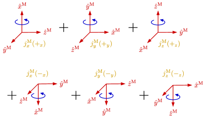
Figure 2: Scheme of the right hand side of Eq. (17) depicting the 6 different orientations of the molecular frame contributing to the net photoelectron current in the lab frame. The curved blue arrows indicate the field in the lab frame. For each orientation only the component of the photoelectron current perpendicular to the polarization plane is taken into account. These orientations are unique only up to a rotation around the axis perpendicular to the polarization plane.

The right hand side of Eq. (16) is depicted in Fig. 1, which shows the different field geometries and the corresponding components of the current in the molecular frame that account for the net current in the lab frame. This figure immediately suggests the equivalent but somewhat more natural picture shown in Fig. 2, where the field geometry is kept fixed and the molecule assumes the six different orientations in which $\hat{x}^{\mathrm{M}}$, $-\hat{x}^{\mathrm{M}}$, $\hat{y}^{\mathrm{M}}$, $-\hat{y}^{\mathrm{M}}$, $\hat{z}^{\mathrm{M}}$, and $-\hat{z}^{\mathrm{M}}$, coincide with $\hat{z}^{\mathrm{L}}$. To reflect this picture Eq. (16) can be rewritten as follows:

$$\vec{j}^{\mathrm{L}}=\left\{\frac{1}{6}\sum_{i=x,y,z}\left[j_{z}^{\mathrm{L}}\left(\sigma,\lambda_{i}\right)+j_{z}^{\mathrm{L}}\left(\sigma,\lambda_{-i}\right)\right]\right\}\hat{z}^{\mathrm{L}},$$ (17)

where $\lambda_{i}$ and $\lambda_{-i}$ are the Euler angles specifying the orientation for which the $i$-th molecular axis is parallel to $\hat{z}^{\mathrm{L}}$ and $-\hat{z}^{\mathrm{L}}$, respectively. This change of picture corresponds to the substitutions: $j_{z}^{\mathrm{L}}\left(\sigma,\lambda_{\pm i}\right)=\pm j_{i}^{\mathrm{M}}\left((\pm\sigma)_{i}\right)$ which directly follow from comparing Figs. 1 and 2. The Euler angles $\lambda_{\pm i}$ are not unique because the $z$ component of the current $\vec{j}^{\mathrm{L}}\left(\sigma,\lambda_{\pm i}\right)$ is of course invariant with respect to rotations of the molecular frame about $\hat{z}^{\mathrm{L}}$, and therefore the specific orientation of the molecular axes that lie on the polarization plane is irrelevant. Furthermore, the definition of the orientation of the molecular frame with respect to the nuclei that form the molecule is also arbitrary. Thus, what Eq. (17) really says is that the orientation-averaged photoelectron current for a randomly-oriented ensemble is equivalent to the average over six molecular orientations, where each orientation corresponds to having one of the six spatial directions in the molecular frame pointing along $\hat{z}^{\mathrm{L}}$.

We can work a bit more on Eq. (17) to avoid the ambiguity of $\lambda_{\pm i}$ mentioned above. If for a given orientation $\lambda_{i}$ the current in the lab frame is $\vec{j}^{\mathrm{L}}\left(\sigma,\lambda_{i}\right)$, then the average of $\vec{j}^{\mathrm{L}}\left(\sigma,\lambda_{i}\right)$ over all the orientations $\lambda_{i}\left(\phi\right)$, that yield the same orientation as $\lambda_{i}$ up to a rotation by $\phi$ of the molecular frame around $\hat{z}^{\mathrm{L}}$, yields the $z$ component of $\vec{j}^{\mathrm{L}}\left(\sigma,\lambda_{i}\right)$, i.e.

$$\frac{1}{2\pi}\int_{0}^{2\pi}\mathrm{d}\phi\vec{j}^{\mathrm{L}}\left(\sigma,\lambda_{i}\left(\phi_{i}\right)\right)=j_{z}^{\mathrm{L}}\left(\sigma,\lambda_{i}\right)\hat{z}^{\mathrm{L}}.$$ (18)

This means that we can rewrite the net orientation-averaged photoelectron current [Eq. (17)] in the more symmetric form

$$\vec{j}^{\mathrm{L}}\left(k\right)=\frac{1}{3}\sum_{i=x,y,z}\frac{1}{2}\left\{\frac{1}{2\pi}\int_{0}^{2\pi}\mathrm{d}\phi\vec{j}^{\mathrm{L}}\left(\lambda_{i}\left(\phi\right)\right)+\frac{1}{2\pi}\int_{0}^{2\pi}\mathrm{d}\phi\vec{j}^{\mathrm{L}}\left(\lambda_{-i}\left(\phi\right)\right)\right\}.$$ (19)

This equation provides the relationship between the isotropically-oriented-ensemble PECD and the aligned-ensemble PECD that we were looking for. The $i$-th term in the summation corresponds to the average photoelectron current that a molecular ensemble yields when its $i$-th molecular axis is perfectly aligned (parallel and anti-parallel) along the normal to the polarization plane, and the other two molecular axes take all possible orientations in the polarization plane. That is, Eq. (19) shows that the net photoelectron current for an isotropically-oriented ensemble is simply the average of the three different aligned-ensemble cases.

IV PECD in aligned molecular ensembles

From Eq. (19) we can infer that the introduction of partial alignment along an axis perpendicular to the polarization plane in an otherwise isotropic ensemble will simply change the weight factors of the aligned-ensemble contributions in favor of the molecular axis which is being aligned. In this section we will confirm that this is indeed the case by deriving an exact formula for the net photoelectron current in the lab frame resulting from photoionization via circularly polarized light of a molecular ensemble exhibiting an arbitrary degree of alignment with respect to the normal to the polarization plane. We will also derive an analogous formula for the case in which the alignment axis is in the plane of polarization, which corresponds to the standard experimental set-up when the laser field used to align the sample co-propagates with the ionizing field. But first we will briefly discuss some general symmetry properties that explain enantiosensitivity and dichroism in these ensembles from a purely geometrical point of view.

IV.1 Symmetry considerations for aligned and oriented ensembles

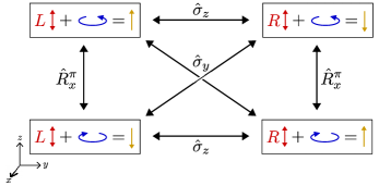
Figure 3: Symmetry properties of an ensemble of chiral molecules interacting with circularly polarized light in the electric-dipole approximation. The ensemble is partially (or totally) aligned along the ($z$) axis perpendicular to the ($xy$) polarization plane of the light. The box represents the “enantiomer+field” system. Inside the box: the red letters $L$ and $R$ specify the enantiomer, the red double-headed vertical arrow specifies the direction along which the molecules are aligned, the blue curved arrow specifies the direction of rotation of a field circularly polarized in the $xy$ plane, and the golden vertical arrow stands for a polar vector observable $\vec{v}=v_{z}\hat{z}$ displaying asymmetry with respect to the polarization plane $xy$. A reflection $\hat{\sigma}_{z}$ with respect to the $xy$ plane, leaves the field invariant, but swaps the enantiomer and flips $\vec{v}$ (enantiosensitivity). A rotation $\hat{R}_{a}^{\pi}$ by $\pi$ radians around any vector $\vec{a}$ contained in the $xy$ plane leaves the enantiomer invariant, but swaps the polarization and flips $\vec{v}$ (dichroism). Note that a rotation $\hat{R}_{x}^{\pi}$ ($\hat{R}_{y}^{\pi}$) followed by a reflection $\hat{\sigma}_{z}$ is equivalent to a reflection $\hat{\sigma}_{y}$ ($\hat{\sigma}_{x}$) and leaves $\vec{v}$ invariant but swaps both the enantiomer and the polarization. Thus, except for very specific cases (see Fig. 4), FBA in aligned ensembles is a signature of molecular chirality (see also Fig. 5).

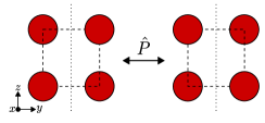
Figure 4: Left: an achiral molecule consisting of four identical atoms with Cartesian coordinates $(-a,-b,b)$, $(a,b,b)$, $(a,-b,-b)$, and $(-a,b,-b)$. Right: spatial inversion of the molecule on the left. A rotation by $\pi/2$ around the $x$ axis yields the molecule on the left. However, molecular alignment restricts available rotations. Thus if we consider a sample aligned along the vertical dotted line, the rotation by $\pi/2$ is not allowed and the aligned sample becomes effectively chiral.

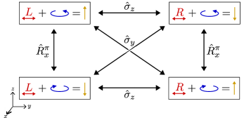
Figure 5: Symmetry properties of an ensemble of chiral molecules interacting with circularly polarized light in the electric-dipole approximation. The ensemble is partially (or totally) aligned along an axis ($y$) contained in the ($xy$) polarization plane of the light. Notations are described in Fig. 3. This shows that, except for very specific cases (see Fig. 4), FBA in aligned ensembles is a signature of molecular chirality (see also Fig. 3).

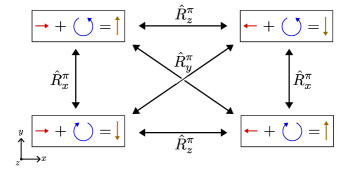
Figure 6: Symmetry considerations for an ensemble of oriented (chiral or achiral) molecules. Notations are described in Fig. 3. The orientation axis ($x$) is in the polarization plane of the light ($xy$). A rotation $\hat{R}_{z}^{\pi}$ by $\pi$ radians around the $z$ axis leaves the field invariant, but flips both the molecular orientation and $v_{y}\hat{y}$ (orientation sensitivity). A rotation $\hat{R}_{x}^{\pi}$ by $\pi$ radians around the $x$ axis leaves the orientation invariant, but swaps the polarization and flips $v_{y}\hat{y}$ (dichroism). Note that a rotation $\hat{R}_{z}^{\pi}$ ($\hat{R}_{x}^{\pi}$) followed by a rotation $\hat{R}_{x}^{\pi}$ ($\hat{R}_{z}^{\pi}$) is equivalent to a rotation $\hat{R}_{y}^{\pi}$ and leaves $v_{y}\hat{y}$ invariant but flips the orientation and the polarization. For achiral molecules reflection symmetry forbids signals perpendicular to the polarization plane, i.e. $v_{z}=0$. For chiral molecules such FBA signal is not symmetry forbidden and it is enantiosensitive and dichroic.

The relevant symmetry properties of an aligned ensemble of chiral molecules interacting with circularly polarized light in the electric-dipole approximation are summarized in Fig. 3 (cf. Fig. 2 in Ordonez and Smirnova (2018b)) for the case of alignment perpendicular to the polarization plane. In this case, the cylindrical symmetry of the “aligned-enantiomer + field” system enforces cylindrical symmetry on the observables and therefore limits the asymmetry of the photoelectron angular distribution to be along the axis perpendicular to the polarization plane, i.e. forward-backward asymmetry (FBA). Furthermore, if the aligned sample is achiral then the “enantiomer + field” system becomes invariant with respect to reflections through the polarization plane, and the forward-backward asymmetry disappears. That is, like in the isotropic case, in the aligned case the FBA is also a signature of the chirality of the sample.

However, unlike in the isotropic case, in the aligned case one must be careful of distinguishing between the chirality of the aligned sample and the chirality of the molecules that make up the sample. Although an aligned sample of chiral molecules is always chiral, a chiral aligned sample is not necessarily made out of chiral molecules. The reason is that restricting the degrees of freedom of the molecular orientation may lead to suppression of the orientation corresponding to the reflection of an allowed orientation and therefore induce chirality. An example of how this may occur is shown in Fig. 4, where we can see that such alignment-induced chirality seems to require a very particular interplay between the molecular symmetry and the alignment axis. In the absence of such particular conditions, alignment does not induces chirality in the sample and FBA can be traced back to the chirality of the molecules.

Figure 5 shows a symmetry diagram analogous to that in Fig. 3 for the setup in which the molecular alignment axis is in the plane of polarization of the ionizing light. In this case the molecular alignment breaks the cylindrical symmetry. Nevertheless the system remains invariant with respect to rotations by $\pi$ around the $z$ axis and the vector observable is again constrained to the $\hat{z}$ direction. Like for the previous case, the dichroic and enantiosensitive FBA is a signature of the chirality of the molecular sample.

It is important to distinguish the FBA discussed here from the dichroic asymmetry observed in Refs. Dubs et al. (1985a, b); Holmegaard et al. (2010) in oriented achiral samples. While the former is with respect to the polarization plane and is a hallmark of the chirality of the sample, the latter is with respect to the plane containing the spin of the photon and the orientation axis (a plane perpendicular to the polarization plane), and takes place even for achiral samples. Figure 6 shows how such dichroic asymmetry can emerge in uniaxially oriented chiral and achiral systems. The $x$ component of $\vec{v}$ is not shown because it is not dichroic and the $z$ component reflecting FBA is zero in achiral systems because of reflection symmetry with respect to the $xy$ plane.

IV.2 Connection between chiral current and molecular field for aligned ensembles

Now that we have established a general starting point based on the symmetry properties of the “aligned-enantiomer + field” system, we will proceed to the derivation of the lab-frame net photoelectron current for such an ensemble for the case of one-photon absorption. The molecular alignment can be introduced in the orientation-averaging procedure via a weight function $w\left(\lambda\right)$ that depends on the Euler angles $\lambda\equiv\alpha\beta\gamma$, which are the angles that determine the relative orientation between the lab frame and the molecular frame. In the ZYZ convention, $\beta$ determines the angle between the $z$ axes of the two frames, so that to describe molecular alignment we can use a distribution $w\left(\beta\right)$ that only depends on this angle and that is symmetric with respect to $\beta=\pi/2$. With the molecular alignment defined along the $\hat{z}^{\mathrm{L}}$ axis (or viceversa), we can consider that the circularly polarized field is in the $x^{\mathrm{L}}y^{\mathrm{L}}$ plane or in the $y^{\mathrm{L}}z^{\mathrm{L}}$ plane, depending on whether we are interested in the setup where the molecular alignment is perpendicular or parallel to the light polarization plane, respectively.

Alignment perpendicular to the plane of polarization

For light circularly polarized in the $x^{\mathrm{L}}y^{\mathrm{L}}$ plane the photoelectron current density in the lab frame corresponding to a given photoelectron momentum $\vec{k}^{\mathrm{M}}$ in the molecular frame and a given molecular orientation $\lambda\equiv(\alpha,\beta,\gamma)$ is Ordonez and Smirnova (2018b)

$$\vec{j}^{\mathrm{L}}\left(\vec{k}^{\mathrm{M}},\lambda\right) =\frac{\left|\tilde{\mathcal{E}}\right|^{2}}{2}\left|\vec{D}^{\mathrm{L}}\cdot\left(\hat{x}^{\mathrm{L}}+\sigma\mathrm{i}\hat{y}^{\mathrm{L}}\right)\right|^{2}\vec{k}^{\mathrm{L}}$$

$$=\frac{\left|\tilde{\mathcal{E}}\right|^{2}}{2}\left[\left|S\vec{D}^{\mathrm{M}}\cdot\hat{x}^{\mathrm{L}}\right|^{2}+\left|S\vec{D}^{\mathrm{M}}\cdot\hat{y}^{\mathrm{L}}\right|^{2}+\sigma\mathrm{i}S\left(\vec{D}^{\mathrm{M}*}\times\vec{D}^{\mathrm{M}}\right)\cdot\hat{z}^{\mathrm{L}}\right]S\vec{k}^{\mathrm{M}},$$ (20)

where $S(\lambda)$ is the rotation matrix that takes vectors from the molecular frame to the lab frame, i.e. $\vec{v}^{\mathrm{L}}=S\left(\lambda\right)\vec{v}^{\mathrm{M}}$, $\tilde{\mathcal{E}}$ is the Fourier transform of the electric field evaluated at the transition frequency, and $\sigma=\pm 1$ stands for left($+$)/right($-$) circularly polarized light. Before moving on to the case at hand, Eq. (20) gives us the opportunity to briefly point out another reason why only the coherent term survives the orientation averaging in both isotropically-oriented and aligned ensembles. For each orientation $\lambda_{i}$ of the molecular frame there will be another orientation $\lambda_{-i}$ related to it by a rotation by $\pi$ around (for example) $\hat{y}^{\mathrm{L}}$ that will change the sign of the $x^{\mathrm{L}}$ and $z^{\mathrm{L}}$ components of all molecular vectors. Therefore, if we consider the average of $j_{z}^{\mathrm{L}}(\vec{k}^{\mathrm{M}},\lambda)$ over those two orientations, $[j_{z}^{\mathrm{L}}(\vec{k}^{\mathrm{M}},\lambda_{i})+j_{z}^{\mathrm{L}}(\vec{k}^{\mathrm{M}},\lambda_{-i})]/2$, we can see from (20) that the incoherent terms $|S\vec{D}^{\mathrm{M}}\cdot\hat{x}^{\mathrm{L}}|^{2}(S\vec{k}^{\mathrm{M}}\cdot\hat{z}^{\mathrm{L}})$ and $|S\vec{D}^{\mathrm{M}}\cdot\hat{y}^{\mathrm{L}}|^{2}(S\vec{k}^{\mathrm{M}}\cdot\hat{z}^{\mathrm{L}})$ will cancel because they have opposite signs for opposite orientations, while the coherent term $\sigma[S(\mathrm{i}\vec{D}^{\mathrm{M}*}\times\vec{D}^{\mathrm{M}})\cdot\hat{z}^{\mathrm{L}}](S\vec{k}^{\mathrm{M}}\cdot\hat{z}^{\mathrm{L}})$ will not because it is the same for both orientations. That is, while obviously each term of $j_{z}^{\mathrm{L}}(\vec{k}^{\mathrm{M}},\lambda)$ is invariant with respect to rotations of the molecular frame by $\pi$ around $\hat{z}^{\mathrm{L}}$, only the coherent term is invariant with respect to rotations by $\pi$ with respect to any axis. Thus, either for isotropically-oriented samples or aligned samples (with molecular alignment perpendicular to the polarization plane or not), the incoherent terms will always cancel by pairs in the orientation averaging while the coherent term term will not.

For a distribution of orientations $w\left(\beta\right)$, the net photoelectron current in the lab frame takes the form:

$$\vec{j}^{\mathrm{L}}\left(k\right) = \int\mathrm{d}\Omega_{k}^{\mathrm{M}}\int\mathrm{d}\lambda w\left(\beta\right)\vec{j}^{\mathrm{L}}\left(\vec{k}^{\mathrm{M}},\lambda\right),$$ (21)

where $\int\mathrm{d}\lambda\equiv\int_{0}^{2\pi}\mathrm{d}\alpha\int_{0}^{\pi}\mathrm{d}\beta\int_{0}^{2\pi}\mathrm{d}\gamma\sin\beta/8\pi^{2}$ is the integral over molecular orientations, and $\int\mathrm{d}\Omega_{k}^{\mathrm{M}}\equiv\int_{0}^{2\pi}\mathrm{d}\phi_{k}^{\mathrm{M}}\int_{0}^{\pi}\mathrm{d}\theta_{k}^{\mathrm{M}}\sin\theta_{k}^{\mathrm{M}}$ is the integral over directions of the photoelectron momentum $\vec{k}^{\mathrm{M}}$. For an alignment distribution $w\left(\beta\right)\propto\cos^{2}\beta$, Eq. (21) becomes equivalent to the photoelectron current found in the case where a pump linearly polarized along $\hat{z}^{\mathrm{L}}$ resonantly excites the molecule via a transition dipole parallel to $\hat{z}^{\mathrm{M}}$ into a bound excited electronic state and is then photoionized from the latter by a circularly polarized probe pulse. Therefore, for such a distribution we could simply make use of Eq. (31) derived in Ordonez and Smirnova (2018b) in the context of the generalized PXECD (see Appendix VII.1). This equivalence reveals the close relation between aligned ensembles where the molecular orientation is anisotropic and isotropically-oriented ensembles that have been electronically excited. This happens because the field imprints its anisotropy on the originally isotropic molecular ensemble via the excitation.

In the following we will make no assumption about $w\left(\beta\right)$ except that it is symmetric with respect to $\beta=\pi/2$, which simply imposes the condition of alignment. The first two terms in Eq. (20) describe interaction with a linearly polarized field and therefore, from symmetry considerations, they lead to $\vec{j}^{\mathrm{L}}\left(k\right)=0$. The integral over orientations of the third term in Eq. (20) can be carried out with the help of Eq. (33) derived in Appendix VII.1 and yields

$$\vec{j}^{\mathrm{L}}\left(k\right)=\frac{\sigma\left|\tilde{\mathcal{E}}\right|^{2}}{2}\bigg{[}\frac{1}{3}w_{i}\int\mathrm{d}\Omega_{k}^{\mathrm{M}}\left(\mathrm{i}\vec{D}^{\mathrm{M}*}\times\vec{D}^{\mathrm{M}}\right)\cdot\vec{k}^{\mathrm{M}}\\ +\left(1-w_{i}\right)\int\mathrm{d}\Omega_{k}^{\mathrm{M}}\left(\mathrm{i}\vec{D}^{\mathrm{M}*}\times\vec{D}^{\mathrm{M}}\right)_{z}k_{z}^{\mathrm{M}}\bigg{]}\hat{z}^{\mathrm{L}},$$ (22)

where we assumed that $w\left(\beta\right)$ is properly normalized [see Eq. (35)] and we defined $w_{i}$ as

$$w_{i}\equiv\frac{3}{4}\int_{0}^{\pi}\mathrm{d}\beta w\left(\beta\right)\sin^{3}\beta.$$ (23)

$w_{i}$ is a parameter determined exclusively by $w(\beta)$. Equation (22) can be written in an equivalent form [cf. Eqs. (4) (9), and (14)]:

$$\vec{j}^{\mathrm{L}}\left(k\right)=\frac{\sigma\left|\tilde{\mathcal{E}}\right|^{2}}{2k}\bigg{[}\frac{1}{3}w_{i}\Phi^{\chi}(k)+\left(1-w_{i}\right)\Phi^{\chi}_{z}(k)\bigg{]}\hat{z}^{\mathrm{L}}.$$ (24)

Table 1 shows $w(\beta)$, $w_{i}$, and $j_{z}^{\mathrm{L}}$ for perfectly aligned, isotropic, and perfectly antialigned samples. While the isotropic case reduces to Eq. (13) and gives the average of $\Phi_{x}^{\chi}$, $\Phi_{y}^{\chi}$, and $\Phi_{z}^{\chi}$ [i.e. the total flux, see Eqs. (9) and (14)], the perfectly aligned case singles out the $\Phi_{z}^{\chi}$, in full agreement with our discussion in Sec. III. On the other hand, the perfectly antialigned case, where the molecular $z$ axis is constrained to be perpendicular to the laboratory $z$ axis, prevents $\Phi_{z}^{\chi}$ from contributing to the photoelectron current.

As shown in Appendix VII.1, for the case $w\left(\beta\right)\propto\cos^{2}\beta$, Eq. (22) coincides with the predictions of the generalized PXECD formula derived in Ordonez and Smirnova (2018b) and discussed above.

			$\tilde{\vec{\mathcal{E}}}=\frac{\tilde{\mathcal{E}}}{\sqrt{2}}\left(\hat{x}+\sigma i\hat{y}\right)$	$\tilde{\vec{\mathcal{E}}}=\frac{\tilde{\mathcal{E}}}{\sqrt{2}}\left(\hat{y}+\sigma i\hat{z}\right)$
	$w\left(\beta\right)$	$w_{i}$	$j_{z}/\frac{\sigma\left|\tilde{\mathcal{E}}\right|^{2}}{2k}$	$j_{x}/\frac{\sigma\left|\tilde{\mathcal{E}}\right|^{2}}{2k}$
aligned	$\frac{2\left[\delta\left(\beta\right)+\delta\left(\beta-\pi\right)\right]}{\sin\beta}$	$0$	$\Phi_{z}$	$\frac{1}{2}\left(\Phi_{x}+\Phi_{y}\right)$
isotropic	$1$	$1$	$\frac{1}{3}\left(\Phi_{x}+\Phi_{y}+\Phi_{z}\right)$	$\frac{1}{3}\left(\Phi_{x}+\Phi_{y}+\Phi_{z}\right)$
antialigned	$\frac{2\delta\left(\beta-\frac{\pi}{2}\right)}{\sin\beta}$	$\frac{3}{2}$	$\frac{1}{2}\left(\Phi_{x}+\Phi_{y}\right)$	$\frac{1}{4}\left(\Phi_{x}+\Phi_{y}+2\Phi_{z}\right)$

Table 1: Photoelectron current density in aligned, isotropic, and antialigned samples for circular polarization perpendicular [fourth column, Eq. (24)] and parallel [fifth column, Eq. (27)] to the alignment axis $z$. We have dropped the L and the $\chi$ superscripts for simplicity.

Alignment parallel to the plane of polarization

The derivation for the setup in which the molecular alignment axis is contained in the polarization plane follows analogously with only subtle differences. This time we define the orientation of the lab frame such that the molecular alignment remains along the $\hat{z}^{\mathrm{L}}$ axis but now the light is polarized in the $y^{\mathrm{L}}z^{\mathrm{L}}$ plane, and therefore we have that the photoelectron current in the lab frame corresponding to a given photoelectron momentum $\vec{k}^{\mathrm{M}}$ in the molecular frame and a given molecular orientation $\lambda\equiv(\alpha,\beta,\gamma)$ reads as

$$\vec{j}^{\mathrm{L}}\left(\vec{k}^{\mathrm{M}},\lambda\right)=\frac{\left|\tilde{\mathcal{E}}\right|^{2}}{2}\left[\left|S\vec{D}^{\mathrm{M}}\cdot\hat{y}^{\mathrm{L}}\right|^{2}+\left|S\vec{D}^{\mathrm{M}}\cdot\hat{z}^{\mathrm{L}}\right|^{2}+\sigma\mathrm{i}S\left(\vec{D}^{\mathrm{M}*}\times\vec{D}^{\mathrm{M}}\right)\cdot\hat{x}^{\mathrm{L}}\right]S\vec{k}^{\mathrm{M}}.$$ (25)

With the help of Eq. (37) derived in Appendix VII.1 we obtain

$$\vec{j}^{\mathrm{L}}\left(k\right)=\frac{\sigma\left|\tilde{\mathcal{E}}\right|^{2}}{2}\bigg{[}\frac{1}{3}\frac{\left(3-w_{i}\right)}{2}\int\mathrm{d}\Omega_{k}^{\mathrm{M}}\left(\mathrm{i}\vec{D}^{\mathrm{M}*}\times\vec{D}^{\mathrm{M}}\right)\cdot\vec{k}^{\mathrm{M}}\\ +\frac{1}{2}\left(w_{i}-1\right)\int\mathrm{d}\Omega_{k}^{\mathrm{M}}\left(\mathrm{i}\vec{D}^{\mathrm{M}*}\times\vec{D}^{\mathrm{M}}\right)_{z}k_{z}^{\mathrm{M}}\bigg{]}\hat{x}^{\mathrm{L}}.$$ (26)

Like in the previous case, and as follows from the symmetry considerations of Sec. IV.1, the current is directed along the direction perpendicular to the polarization plane of the incident field. Comparing with Eq. (22) we can see that the factors in front of the isotropic and anisotropic contributions are slightly different from what we obtained in the previous case. We can rewrite this equation in an equivalent form [cf. Eqs. (4), (9), and (14)]:

$$\vec{j}^{\mathrm{L}}\left(k\right)=\frac{\sigma\left|\tilde{\mathcal{E}}\right|^{2}}{2k}\bigg{[}\frac{1}{3}\frac{\left(3-w_{i}\right)}{2}\Phi^{\chi}(k)+\frac{1}{2}\left(w_{i}-1\right)\Phi^{\chi}_{z}(k)\bigg{]}\hat{x}^{\mathrm{L}}.$$ (27)

Some limiting cases of this equation are shown in the last column of Table 1, where we can see that, as expected, this formula reduces to Eq. (13) in the isotropic case. We can also see that the aligned case with the alignment parallel to the polarization plane yields the same result as the antialigned case with the alignment perpendicular to the polarization plane, as expected from symmetry, and that antialignment doubles the weight of $\Phi_{z}^{\chi}$ with respect to that of $\Phi_{x}^{\chi}$ and $\Phi_{y}^{\chi}$. Appendix VII.1 shows how Eq. (26) can also be derived from the generalized PXECD formulas derived in Ordonez and Smirnova (2018b) when $w\left(\beta\right)\propto\cos^{2}\beta$.

Equations (24) and (27) suggest that choosing the alignment properly could lead to an increase of the PECD signal. Such increase has been recently discovered both theoretically and experimentally in Ref. Tia et al. (2017). The increase can be rationalized in terms of the propensity field $\vec{B}^{\mathrm{M}}(\vec{k}^{\mathrm{M}})$ and its strength along different $\vec{k}^{\mathrm{M}}$ directions. For example, if a molecule is such that $|\Phi^{\chi}_{z}|>|\Phi^{\chi}_{x}|$ and $|\Phi^{\chi}_{z}|>|\Phi^{\chi}_{y}|$, and the $z$ molecular axis can be aligned, then Eq. (24) shows that the PECD signal will increase with the alignment. Similarly, if for example $\Phi^{\chi}_{z}$ has an opposite sign to that of $\Phi^{\chi}_{x}$ and $\Phi^{\chi}_{y}$, then Eq. (24) shows that the PECD signal will also benefit from the alignment.

V Conclusions

The enantiosensitive photoelectron current, or in other words, the forward-backward asymmetry in photoelectron circular dichroism (PECD), is determined by the the propensity field, which is analogous to the Berry curvature in a two-band solid. This field is independent of light properties, is defined in the molecular frame, and is unique to each molecule. The enantiosensitive photoelectron current stemming from aligned ensembles of chiral molecules is only sensitive to specific components of the propensity field and therefore the increase or decrease of the chiral response vs. molecular alignment depends on the structure of this field. Each component of the propensity field reflects photoelectron-momentum-resolved absorption circular dichroism and is only non-zero in the absence of rotational symmetry about the corresponding axis. The propensity field underlies the emergence of PECD. Thus, in this paper we have generalized the ideas presented in our companion paper Ordonez and Smirnova (2018a), which illustrates the role of optical propensity rules in PECD in aligned molecular ensembles for specific examples of chiral states.

In the case of unaligned molecular ensembles, the enantiosensitive photoelectron current for a given absolute value $k$ of the photoelectron momentum is proportional to the flux of the propensity field through the sphere of radius $k$. The flux is a pseudoscalar and has opposite sign for opposite enantiomers. Molecular alignment allows one to probe the flux generated by specific components of the propensity field.

VI Acknowledgements

The authors thank Alvaro Jiménez-Galán, Rui Silva, David Ayuso and Misha Ivanov for illuminating discussions and essential collaboration on this topic. The authors gratefully acknowledge the MEDEA project, which has received funding from the European Union’s Horizon 2020 research and innovation programme under the Marie Skłodowska-Curie grant agreement 641789. The authors gratefully acknowledge support from the DFG SPP 1840 “Quantum Dynamics in Tailored Intense Fields” and DFG grant SM 292/5-2.

VII Appendix

VII.1 Orientation averaging in aligned ensembles

In this appendix we will derive the orientation averaged net photoelectron current in the lab frame for the aligned ensembles considered in Sec. (IV.2). Before deriving the expression for an arbitrary distribution $w(\beta)$, we will consider the particular distribution $w\left(\beta\right)=3\cos^{2}\beta$ in order to draw some connections between the results obtained in a randomly oriented sample and an aligned sample. In this case the net photoelectron current can be written as [see Eqs. (20) and (21)]

$$\vec{j}^{\mathrm{L}}\left(k\right) = 3\int\mathrm{d}\Omega_{k}^{\mathrm{M}}\int\mathrm{d}\lambda\cos^{2}\beta\,\vec{j}^{\mathrm{L}}\left(\vec{k}^{\mathrm{M}},\lambda\right)$$

$$= 3\int\mathrm{d}\Omega_{k}^{\mathrm{M}}\int\mathrm{d}\lambda\,\left|\hat{d}_{\mathrm{eff}}^{\mathrm{L}}\cdot\hat{\tilde{\mathcal{E}}}_{\mathrm{eff}}^{\mathrm{L}}\right|^{2}\left|\vec{D}^{\mathrm{L}}\cdot\vec{\tilde{\mathcal{E}}}^{\mathrm{L}}\right|^{2}\vec{k}^{\mathrm{L}},$$

which simply shows that the anisotropic orientation average of $\vec{j}^{\mathrm{L}}(\vec{k}^{\mathrm{M}},\lambda)$ is equivalent to the isotropic averaging of $|\hat{d}_{\mathrm{p}}^{\mathrm{L}}\cdot\hat{\tilde{\mathcal{E}}}_{\mathrm{p}}^{\mathrm{L}}|^{2}|\vec{D}^{\mathrm{L}}\cdot\vec{\tilde{\mathcal{E}}}^{\mathrm{L}}|^{2}$, where we introduced an effective bound-bound transition dipole $\hat{d}_{\mathrm{eff}}^{\mathrm{M}}=\hat{z}^{\mathrm{M}}$ and the effective field which interacts with it $\hat{\tilde{\mathcal{E}}}_{\mathrm{eff}}^{\mathrm{L}}=\hat{z}^{\mathrm{L}}$, in order to make evident that, mathematically, we are dealing with a particular case of the generalized PXECD effect considered in Ordonez and Smirnova (2018b), where first a pump pulse of arbitrary polarization excites the system into a superposition of two excited states and then a probe pulse of arbitrary polarization photoionizes the system from intermediate state. In the present case the effective pump pulse excites the system from an effective ground state into a single excited state (the actual ground state) through the interaction $\hat{d}_{\mathrm{eff}}^{\mathrm{L}}\cdot\hat{\tilde{\mathcal{E}}}_{\mathrm{eff}}^{\mathrm{L}}$ and then the probe pulse (the actual pulse) photoionizes the system from the excited state. That is, we only have to deal with Eq. (31) in Ordonez and Smirnova (2018b), which in our case reads as

$$\vec{j}^{\mathrm{L}}\left(k\right) =3\int\mathrm{d}\Omega_{k}^{\mathrm{M}}\int\mathrm{d}\lambda\,\left|\hat{d}_{\mathrm{eff}}^{\mathrm{L}}\cdot\hat{\tilde{\mathcal{E}}}_{\mathrm{eff}}^{\mathrm{L}}\right|^{2}\left|\vec{D}^{\mathrm{L}}\cdot\vec{\tilde{\mathcal{E}}}^{\mathrm{L}}\right|^{2}\vec{k}^{\mathrm{L}}$$

$$=\frac{1}{5}\Re\bigg{\{}\int\mathrm{d}\Omega_{k}^{\mathrm{M}}\left[\left(\hat{d}_{\mathrm{eff}}^{\mathrm{M}}\times\vec{D}^{\mathrm{M}*}\right)\cdot\vec{D}^{\mathrm{M}}\right]\left(\hat{d}_{\mathrm{eff}}^{\mathrm{M}}\cdot\vec{k}^{\mathrm{M}}\right)\left[\left(\hat{\tilde{\mathcal{E}}}_{\mathrm{eff}}^{\mathrm{L}}\times\tilde{\vec{\mathcal{E}}}^{\mathrm{L}*}\right)\cdot\tilde{\vec{\mathcal{E}}}^{\mathrm{L}}\right]\hat{\tilde{\mathcal{E}}}_{\mathrm{eff}}^{\mathrm{L}}$$

$$+\int\mathrm{d}\Omega_{k}^{\mathrm{M}}\left[\left(\hat{d}_{\mathrm{eff}}^{\mathrm{M}}\times\vec{D}^{\mathrm{M}*}\right)\cdot\vec{k}^{\mathrm{M}}\right]\left(\hat{d}_{\mathrm{eff}}^{\mathrm{M}}\cdot\vec{D}^{\mathrm{M}}\right)\left(\hat{\tilde{\mathcal{E}}}_{\mathrm{eff}}^{\mathrm{L}}\cdot\tilde{\vec{\mathcal{E}}}^{\mathrm{L}}\right)\left(\hat{\tilde{\mathcal{E}}}_{\mathrm{eff}}^{\mathrm{L}}\times\tilde{\vec{\mathcal{E}}}^{\mathrm{L}*}\right)$$

$$+\int\mathrm{d}\Omega_{k}^{\mathrm{M}}\left[\left(\hat{d}_{\mathrm{eff}}^{\mathrm{M}}\times\vec{D}^{\mathrm{M}}\right)\cdot\vec{k}^{\mathrm{M}}\right]\left(\hat{d}_{\mathrm{eff}}^{\mathrm{M}}\cdot\vec{D}^{\mathrm{M}*}\right)\left(\hat{\tilde{\mathcal{E}}}_{\mathrm{eff}}^{\mathrm{L}}\cdot\tilde{\vec{\mathcal{E}}}^{\mathrm{L}*}\right)\left(\hat{\tilde{\mathcal{E}}}_{\mathrm{eff}}^{\mathrm{L}}\times\tilde{\vec{\mathcal{E}}}^{\mathrm{L}}\right)\bigg{\}}$$

$$+\frac{1}{10}\int\mathrm{d}\Omega_{k}^{\mathrm{M}}\left[\left(\vec{D}^{\mathrm{M}*}\times\vec{D}^{\mathrm{M}}\right)\cdot\vec{k}^{\mathrm{M}}\right]\left(\tilde{\vec{\mathcal{E}}}^{\mathrm{L}*}\times\tilde{\vec{\mathcal{E}}}^{\mathrm{L}}\right),$$ (28)

If the molecular alignment (which we have already set along $\hat{z}^{\mathrm{L}}$) is perpendicular to the polarization plane we set $\tilde{\vec{\mathcal{E}}}^{\mathrm{L}}=\left(\hat{x}^{\mathrm{L}}+\sigma\mathrm{i}\hat{y}^{\mathrm{L}}\right)/\sqrt{2}$. The second and third terms vanish because $(\hat{\tilde{\mathcal{E}}}_{\mathrm{eff}}^{\mathrm{L}}\cdot\tilde{\vec{\mathcal{E}}}^{\mathrm{L}})=0$ and Eq. (28) yields

$$\vec{j}^{\mathrm{L}}\left(k\right)=\frac{\sigma\left|\tilde{\mathcal{E}}\right|^{2}}{2}\bigg{\{}\frac{1}{5}\int\mathrm{d}\Omega_{k}^{\mathrm{M}}\left[\left(\mathrm{i}\vec{D}^{\mathrm{M}*}\times\vec{D}^{\mathrm{M}}\right)\cdot\vec{k}^{\mathrm{M}}\right]\\ +\frac{2}{5}\int\mathrm{d}\Omega_{k}^{\mathrm{M}}\left[\left(\mathrm{i}\vec{D}^{\mathrm{M}*}\times\vec{D}^{\mathrm{M}}\right)_{z}k_{z}^{\mathrm{M}}\right]\bigg{\}}\hat{z}^{\mathrm{L}},$$ (29)

On the other hand, for the case in which molecular alignment is in the plane of the light polarization we set $\tilde{\vec{\mathcal{E}}}^{\mathrm{L}}=\left(\hat{y}^{\mathrm{L}}+\sigma\mathrm{i}\hat{z}^{\mathrm{L}}\right)/\sqrt{2}$. The first term vanishes because $[(\hat{\tilde{\mathcal{E}}}_{\mathrm{eff}}^{\mathrm{L}}\times\tilde{\vec{\mathcal{E}}}^{\mathrm{L}*})\cdot\tilde{\vec{\mathcal{E}}}^{\mathrm{L}}]=0$, and with the help of the vector identities $(\vec{a}\times\vec{b})\cdot(\vec{c}\times\vec{d})$$=(\vec{a}\cdot\vec{c})(\vec{b}\cdot\vec{d})$$-(\vec{a}\cdot\vec{d})(\vec{b}\cdot\vec{c})$ and $(\vec{a}\times\vec{b})\times\vec{c}=$$(\vec{a}\cdot\vec{c})\vec{b}-(\vec{b}\cdot\vec{c})\vec{a}$ we obtain

$$\vec{j}^{\mathrm{L}}\left(k\right)=\frac{\sigma\left|\tilde{\mathcal{E}}\right|^{2}}{2}\bigg{\{}\frac{2}{5}\int\mathrm{d}\Omega_{k}^{\mathrm{M}}\left[\left(\mathrm{i}\vec{D}^{\mathrm{M}*}\times\vec{D}^{\mathrm{M}}\right)\cdot\vec{k}^{\mathrm{M}}\right]\\ -\frac{1}{5}\int\mathrm{d}\Omega_{k}^{\mathrm{M}}\left(\mathrm{i}\vec{D}^{\mathrm{M}*}\times\vec{D}^{\mathrm{M}}\right)_{z}k_{z}^{\mathrm{M}}\bigg{\}}\hat{x}^{\mathrm{L}}.$$ (30)

In both cases, Eq. (29) and (30) show that $\vec{j}^{\mathrm{L}}\left(k\right)$ is along the direction perpendicular to the light polarization plane and that there is an imbalance in the scalar product $(\mathrm{i}\vec{D}^{\mathrm{M}*}\times\vec{D}^{\mathrm{M}})\cdot\vec{k}^{\mathrm{M}}$ that singles out the molecular axis being aligned. Equations (29) and (30) coincide with Eqs. (22) and (26), respectively, when we set $w\left(\beta\right)=3\cos^{2}\beta$ and consequently $w_{i}=3/5$ in Eqs. (22) and (26).

Now we proceed to the general derivation where the only assumption on $w\left(\beta\right)$ is that it is symmetric with respect to $\beta=\pi/2$, which simply imposes the condition of alignment. Since symmetry implies that the incoherent terms corresponding to linear polarization along $\hat{x}^{\mathrm{L}}$ and $\hat{y}^{\mathrm{L}}$ in Eq. (20) vanish, we will focus exclusively on the coherent term. For the case in which the molecular alignment is perpendicular to the light polarization plane, the relevant integral over orientations is of the form [see Eq. (20)]

$$\int\mathrm{d}\lambda\,w\left(\beta\right)\left(\vec{a}^{\mathrm{L}}\cdot\hat{z}^{\mathrm{L}}\right)\vec{b}^{\mathrm{L}},$$ (31)

where $\int\mathrm{d}\lambda\equiv\int_{0}^{2\pi}\mathrm{d}\alpha\int_{0}^{\pi}\mathrm{d}\beta\int_{0}^{2\pi}\mathrm{d}\gamma\,\sin\beta/8\pi^{2}$, $\vec{a}$ and $\vec{b}$ are vectors fixed in the molecular frame. To transform a vector from the molecular frame to the lab frame we use $\vec{v}^{\mathrm{L}}=R\left(\lambda\right)\vec{v}^{\mathrm{M}}$, where

$$R\left(\lambda\right)=\left(\begin{array}[]{ccc}-\mathrm{s}\alpha\,\mathrm{s}\gamma+\mathrm{c}\alpha\,\mathrm{c}\beta\,\mathrm{c}\gamma&-\mathrm{s}\alpha\,\mathrm{c}\gamma-\mathrm{s}\gamma\,\mathrm{c}\alpha\,\mathrm{c}\beta&\mathrm{s}\beta\,\mathrm{c}\alpha\\ \mathrm{s}\alpha\,\mathrm{c}\beta\,\mathrm{c}\gamma+\mathrm{s}\gamma\,\mathrm{c}\alpha&-\mathrm{s}\alpha\,\mathrm{s}\gamma\,\mathrm{c}\beta+\mathrm{c}\alpha\,\mathrm{c}\gamma&\mathrm{s}\alpha\,\mathrm{s}\beta\\ -\mathrm{s}\beta\,\mathrm{c}\gamma&\mathrm{s}\beta\,\mathrm{s}\gamma&\mathrm{c}\beta\end{array}\right),$$ (32)

and s and c stand for $\sin$ and $\cos$, respectively. With the help of $R\left(\lambda\right)$ we calculate the expression $\left(\vec{a}^{\mathrm{L}}\cdot\hat{z}^{\mathrm{L}}\right)\vec{b}^{\mathrm{L}}$ in terms of the molecular frame components of $\vec{a}$ and $\vec{b}$ and then note that most of the terms vanish after integration over $\alpha$ and $\gamma$. The non-vanishing terms read as

$$\int\mathrm{d}\lambda\,w\left(\beta\right)\left(\vec{a}^{\mathrm{L}}\cdot\hat{z}^{\mathrm{L}}\right)\vec{b}^{\mathrm{L}}$$ (33)

$$= \bigg{\{}\left[\int\mathrm{d}\lambda w\left(\beta\right)\sin^{2}\beta\cos^{2}\gamma\right]a_{x}^{\mathrm{M}}b_{x}^{\mathrm{M}}+\left[\int\mathrm{d}\lambda w\left(\beta\right)\sin^{2}\beta\sin^{2}\gamma\right]a_{y}^{\mathrm{M}}b_{y}^{\mathrm{M}}$$

$$+\left[\int\mathrm{d}\lambda w\left(\beta\right)\cos^{2}\beta\right]a_{z}^{\mathrm{M}}b_{z}^{\mathrm{M}}\bigg{\}}\hat{z}^{\mathrm{L}}$$

$$= \bigg{\{}\left[\frac{1}{2}\int_{0}^{\pi}\mathrm{d}\beta w\left(\beta\right)\sin^{3}\beta\right]\frac{1}{2}\left(a_{x}^{\mathrm{M}}b_{x}^{\mathrm{M}}+a_{y}^{\mathrm{M}}b_{y}^{\mathrm{M}}\right)$$

$$+\left[\frac{1}{2}\int_{0}^{\pi}\mathrm{d}\beta w\left(\beta\right)\sin\beta\cos^{2}\beta\right]a_{z}^{\mathrm{M}}b_{z}^{\mathrm{M}}\bigg{\}}\hat{z}^{\mathrm{L}}$$

$$= \left[\frac{1}{3}w_{i}\left(\vec{a}^{\mathrm{M}}\cdot\vec{b}^{\mathrm{M}}\right)+\left(1-w_{i}\right)a_{z}^{\mathrm{M}}b_{z}^{\mathrm{M}}\right]\hat{z}^{\mathrm{L}},$$

where we defined

$$w_{i}\equiv\frac{3}{4}\int_{0}^{\pi}\mathrm{d}\beta w\left(\beta\right)\sin^{3}\beta,$$ (34)

and we assumed that $w\left(\beta\right)$ is normalized so that $\int\mathrm{d}\lambda w\left(\beta\right)=1$, which implies that

$$\frac{1}{2}\int_{0}^{\pi}\mathrm{d}\beta\sin(\beta)w(\beta)=1.$$ (35)

In the case in which molecular alignment is in the plane of the light polarization the relevant integral is of the form [see Eq. (25)]

$$\int\mathrm{d}\lambda\,w\left(\beta\right)\left(\vec{a}^{\mathrm{L}}\cdot\hat{x}^{\mathrm{L}}\right)\vec{b}^{\mathrm{L}},$$ (36)

and we proceed analogously as before to find that the only terms that do not vanish after integration yield

$$\int\mathrm{d}\lambda\,w\left(\beta\right)\left(\vec{a}^{\mathrm{L}}\cdot\hat{x}^{\mathrm{L}}\right)\vec{b}^{\mathrm{L}}$$ (37)

$$= \frac{1}{2}\int_{0}^{\pi}\mathrm{d}\beta\sin\beta\,w\left(\beta\right)\left[\frac{1}{4}\left(1+\cos^{2}\beta\right)\left(a_{x}^{\mathrm{M}}b_{x}^{\mathrm{M}}+a_{y}^{\mathrm{M}}b_{y}^{\mathrm{M}}\right)+\frac{1}{2}\sin^{2}\beta a_{z}^{\mathrm{M}}b_{z}^{\mathrm{M}}\right]\hat{x}^{\mathrm{L}}$$

$$= \frac{1}{2}\int_{0}^{\pi}\mathrm{d}\beta\sin\beta\,w\left(\beta\right)\left[\frac{1}{4}\left(2-\sin^{2}\beta\right)\vec{a}^{\mathrm{M}}\cdot\vec{b}^{\mathrm{M}}-\frac{1}{4}\left(2-3\sin^{2}\beta\right)a_{z}^{\mathrm{M}}b_{z}^{\mathrm{M}}\right]\hat{x}^{\mathrm{L}}$$

$$= \left[\frac{1}{2}\left(1-\frac{w_{i}}{3}\right)\vec{a}^{\mathrm{M}}\cdot\vec{b}^{\mathrm{M}}-\frac{1}{2}\left(1-w_{i}\right)a_{z}^{\mathrm{M}}b_{z}^{\mathrm{M}}\right]\hat{x}^{\mathrm{L}}.$$

References

- Ordonez and Smirnova (2018a) A. F. Ordonez and O. Smirnova, arXiv:1806.09049 [physics, physics:quant-ph] (2018a), arXiv: 1806.09049.
- Ritchie (1976) B. Ritchie, Physical Review A 13, 1411 (1976).
- Powis (2000a) I. Powis, The Journal of Chemical Physics 112, 301 (2000a).
- Böwering et al. (2001) N. Böwering, T. Lischke, B. Schmidtke, N. Müller, T. Khalil, and U. Heinzmann, Physical Review Letters 86, 1187 (2001).
- Condon (1937) E. U. Condon, Reviews of Modern Physics 9, 432 (1937).
- Ordonez and Smirnova (2018b) A. F. Ordonez and O. Smirnova, Physical Review A 98, 063428 (2018b).
- Patterson et al. (2013) D. Patterson, M. Schnell, and J. M. Doyle, Nature 497, 475 (2013).
- Patterson and Doyle (2013) D. Patterson and J. M. Doyle, Physical Review Letters 111, 023008 (2013).
- Yachmenev and Yurchenko (2016) A. Yachmenev and S. N. Yurchenko, Phys. Rev. Lett. 117, 033001 (2016).
- Eibenberger et al. (2017) S. Eibenberger, J. Doyle, and D. Patterson, Phys. Rev. Lett. 118, 123002 (2017).
- Fischer et al. (2001) P. Fischer, A. D. Buckingham, and A. C. Albrecht, Phys. Rev. A 64, 053816 (2001).
- Beaulieu et al. (2018) S. Beaulieu, A. Comby, D. Descamps, B. Fabre, G. A. Garcia, R. Géneaux, A. G. Harvey, F. Légaré, Z. Masín, L. Nahon, A. F. Ordonez, S. Petit, B. Pons, Y. Mairesse, O. Smirnova, and V. Blanchet, Nature Physics 14, 484 (2018).
- Garcia et al. (2003) G. A. Garcia, L. Nahon, M. Lebech, J.-C. Houver, D. Dowek, and I. Powis, The Journal of Chemical Physics 119, 8781 (2003), https://doi.org/10.1063/1.1621379 .
- Turchini et al. (2004) S. Turchini, N. Zema, G. Contini, G. Alberti, M. Alagia, S. Stranges, G. Fronzoni, M. Stener, P. Decleva, and T. Prosperi, Phys. Rev. A 70, 014502 (2004).
- Hergenhahn et al. (2004) U. Hergenhahn, E. E. Rennie, O. Kugeler, S. Marburger, T. Lischke, I. Powis, and G. Garcia, The Journal of Chemical Physics 120, 4553 (2004), https://doi.org/10.1063/1.1651474 .
- Lischke et al. (2004) T. Lischke, N. Böwering, B. Schmidtke, N. Müller, T. Khalil, and U. Heinzmann, Phys. Rev. A 70, 022507 (2004).
- Stranges et al. (2005) S. Stranges, S. Turchini, M. Alagia, G. Alberti, G. Contini, P. Decleva, G. Fronzoni, M. Stener, N. Zema, and T. Prosperi, The Journal of Chemical Physics 122, 244303 (2005), https://doi.org/10.1063/1.1940632 .
- Giardini et al. (2005) A. Giardini, D. Catone, S. Stranges, M. Satta, M. Tacconi, S. Piccirillo, S. Turchini, N. Zema, G. Contini, T. Prosperi, P. Decleva, D. D. Tommaso, G. Fronzoni, M. Stener, A. Filippi, and M. Speranza, ChemPhysChem 6, 1164 (2005), https://onlinelibrary.wiley.com/doi/pdf/10.1002/cphc.200400483 .
- Harding et al. (2005) C. J. Harding, E. Mikajlo, I. Powis, S. Barth, S. Joshi, V. Ulrich, and U. Hergenhahn, The Journal of Chemical Physics 123, 234310 (2005), https://doi.org/10.1063/1.2136150 .
- Nahon et al. (2006) L. Nahon, G. A. Garcia, C. J. Harding, E. Mikajlo, and I. Powis, The Journal of Chemical Physics 125, 114309 (2006).
- Contini et al. (2007) G. Contini, N. Zema, S. Turchini, D. Catone, T. Prosperi, V. Carravetta, P. Bolognesi, L. Avaldi, and V. Feyer, The Journal of Chemical Physics 127, 124310 (2007), https://doi.org/10.1063/1.2779324 .
- Garcia et al. (2008) G. A. Garcia, L. Nahon, C. J. Harding, and I. Powis, Phys. Chem. Chem. Phys. 10, 1628 (2008).
- Ulrich et al. (2008) V. Ulrich, S. Barth, S. Joshi, U. Hergenhahn, E. Mikajlo, C. J. Harding, and I. Powis, The Journal of Physical Chemistry A 112, 3544 (2008).
- Powis et al. (2008a) I. Powis, C. J. Harding, G. A. Garcia, and L. Nahon, ChemPhysChem 9, 475 (2008a), https://onlinelibrary.wiley.com/doi/pdf/10.1002/cphc.200700748 .
- Powis et al. (2008b) I. Powis, C. J. Harding, S. Barth, S. Joshi, V. Ulrich, and U. Hergenhahn, Phys. Rev. A 78, 052501 (2008b).
- Turchini et al. (2009) S. Turchini, D. Catone, G. Contini, N. Zema, S. Irrera, M. Stener, D. D. Tommaso, P. Decleva, and T. Prosperi, ChemPhysChem 10, 1839 (2009).
- Garcia et al. (2010) G. A. Garcia, H. Soldi-Lose, L. Nahon, and I. Powis, The Journal of Physical Chemistry A 114, 847 (2010), pMID: 20038111, https://doi.org/10.1021/jp909344r .
- Nahon et al. (2010) L. Nahon, G. A. Garcia, H. Soldi-Lose, S. Daly, and I. Powis, Phys. Rev. A 82, 032514 (2010).
- Daly et al. (2011) S. Daly, I. Powis, G. A. Garcia, H. Soldi-Lose, and L. Nahon, The Journal of Chemical Physics 134, 064306 (2011), https://doi.org/10.1063/1.3536500 .
- Catone et al. (2012) D. Catone, M. Stener, P. Decleva, G. Contini, N. Zema, T. Prosperi, V. Feyer, K. C. Prince, and S. Turchini, Phys. Rev. Lett. 108, 083001 (2012).
- Catone et al. (2013) D. Catone, S. Turchini, M. Stener, P. Decleva, G. Contini, T. Prosperi, V. Feyer, K. C. Prince, and N. Zema, Rendiconti Lincei 24, 269 (2013).
- Garcia et al. (2013) G. A. Garcia, L. Nahon, S. Daly, and I. Powis, Nature Communications 4 (2013), 10.1038/ncomms3132.
- Turchini et al. (2013) S. Turchini, D. Catone, N. Zema, G. Contini, T. Prosperi, P. Decleva, M. Stener, F. Rondino, S. Piccirillo, K. C. Prince, and M. Speranza, ChemPhysChem 14, 1723 (2013).
- Tia et al. (2013) M. Tia, B. Cunha de Miranda, S. Daly, F. Gaie-Levrel, G. A. Garcia, I. Powis, and L. Nahon, The Journal of Physical Chemistry Letters 4, 2698 (2013), https://doi.org/10.1021/jz4014129 .
- Powis et al. (2014) I. Powis, S. Daly, M. Tia, B. Cunha de Miranda, G. A. Garcia, and L. Nahon, Phys. Chem. Chem. Phys. 16, 467 (2014).
- Tia et al. (2014) M. Tia, B. Cunha de Miranda, S. Daly, F. Gaie-Levrel, G. A. Garcia, L. Nahon, and I. Powis, The Journal of Physical Chemistry A 118, 2765 (2014), pMID: 24654892, https://doi.org/10.1021/jp5016142 .
- Nahon et al. (2016) L. Nahon, L. Nag, G. A. Garcia, I. Myrgorodska, U. Meierhenrich, S. Beaulieu, V. Wanie, V. Blanchet, R. Geneaux, and I. Powis, Phys. Chem. Chem. Phys. 18, 12696 (2016).
- Garcia et al. (2016) G. A. Garcia, H. Dossmann, L. Nahon, S. Daly, and I. Powis, ChemPhysChem 18, 500 (2016), https://onlinelibrary.wiley.com/doi/pdf/10.1002/cphc.201601250 .
- Catone et al. (2017) D. Catone, S. Turchini, G. Contini, T. Prosperi, M. Stener, P. Decleva, and N. Zema, Chemical Physics 482, 294 (2017), electrons and nuclei in motion - correlation and dynamics in molecules (on the occasion of the 70th birthday of Lorenz S. Cederbaum).
- Cherepkov (1982) N. A. Cherepkov, Chemical Physics Letters 87, 344 (1982).
- Powis (2000b) I. Powis, The Journal of Physical Chemistry A 104, 878 (2000b).
- Stener et al. (2004) M. Stener, G. Fronzoni, D. D. Tomasso, and P. Decleva, The Journal of Chemical Physics 120, 3284 (2004).
- Harding and Powis (2006) C. J. Harding and I. Powis, The Journal of Chemical Physics 125, 234306 (2006), https://doi.org/10.1063/1.2402175 .
- Tommaso et al. (2006) D. D. Tommaso, M. Stener, G. Fronzoni, and P. Decleva, ChemPhysChem 7, 924 (2006), https://onlinelibrary.wiley.com/doi/pdf/10.1002/cphc.200500602 .
- Stener et al. (2006) M. Stener, D. Di Tommaso, G. Fronzoni, P. Decleva, and I. Powis, The Journal of Chemical Physics 124, 024326 (2006).
- Dreissigacker and Lein (2014) I. Dreissigacker and M. Lein, Physical Review A 89, 053406 (2014).
- Artemyev et al. (2015) A. N. Artemyev, A. D. Müller, D. Hochstuhl, and P. V. Demekhin, The Journal of Chemical Physics 142, 244105 (2015), https://doi.org/10.1063/1.4922690 .
- Goetz et al. (2017) R. E. Goetz, T. A. Isaev, B. Nikoobakht, R. Berger, and C. P. Koch, The Journal of Chemical Physics 146, 024306 (2017).
- Ilchen et al. (2017) M. Ilchen, G. Hartmann, P. Rupprecht, A. N. Artemyev, R. N. Coffee, Z. Li, H. Ohldag, H. Ogasawara, T. Osipov, D. Ray, P. Schmidt, T. J. A. Wolf, A. Ehresmann, S. Moeller, A. Knie, and P. V. Demekhin, Phys. Rev. A 95, 053423 (2017).
- Tia et al. (2017) M. Tia, M. Pitzer, G. Kastirke, J. Gatzke, H.-K. Kim, F. Trinter, J. Rist, A. Hartung, D. Trabert, J. Siebert, K. Henrichs, J. Becht, S. Zeller, H. Gassert, F. Wiegandt, R. Wallauer, A. Kuhlins, C. Schober, T. Bauer, N. Wechselberger, P. Burzynski, J. Neff, M. Weller, D. Metz, M. Kircher, M. Waitz, J. B. Williams, L. P. H. Schmidt, A. D. Müller, A. Knie, A. Hans, L. Ben Ltaief, A. Ehresmann, R. Berger, H. Fukuzawa, K. Ueda, H. Schmidt-Böcking, R. Dörner, T. Jahnke, P. V. Demekhin, and M. Schöffler, The Journal of Physical Chemistry Letters 8, 2780 (2017), pMID: 28582620, https://doi.org/10.1021/acs.jpclett.7b01000 .
- Daly et al. (2017) S. Daly, I. Powis, G. A. Garcia, M. Tia, and L. Nahon, The Journal of Chemical Physics 147, 013937 (2017), https://doi.org/10.1063/1.4983139 .
- Miles et al. (2017) J. Miles, D. Fernandes, A. Young, C. Bond, S. Crane, O. Ghafur, D. Townsend, J. Sá, and J. Greenwood, Analytica Chimica Acta 984, 134 (2017).
- Lux et al. (2012) C. Lux, M. Wollenhaupt, T. Bolze, Q. Liang, J. Koehler, C. Sarpe, and T. Baumert, Angewandte Chemie International Edition 51, 5001 (2012).
- Lehmann et al. (2013) C. S. Lehmann, R. B. Ram, I. Powis, and M. H. M. Jansenn, The Journal of Chemical Physics 139, 234307 (2013).
- Rafiee Fanood et al. (2014) M. M. Rafiee Fanood, I. Powis, and M. H. M. Janssen, The Journal of Physical Chemistry A 118, 11541 (2014), pMID: 25402546, https://doi.org/10.1021/jp5113125 .
- Rafiee Fanood et al. (2015) M. M. Rafiee Fanood, M. H. M. Janssen, and I. Powis, Phys. Chem. Chem. Phys. 17, 8614 (2015).
- Lux et al. (2015) C. Lux, M. Wollenhaupt, C. Sarpe, and T. Baumert, ChemPhysChem 16, 115 (2015).
- Lux et al. (2016) C. Lux, A. Senftleben, C. Sarpe, M. Wollenhaupt, and T. Baumert, Journal of Physics B: Atomic, Molecular and Optical Physics 49, 02LT01 (2016).
- Fanood et al. (2016) M. M. R. Fanood, M. H. M. Janssen, and I. Powis, The Journal of Chemical Physics 145, 124320 (2016).
- Kastner et al. (2016) A. Kastner, C. Lux, T. Ring, S. Züllighoven, C. Sarpe, A. Senftleben, and T. Baumert, ChemPhysChem 17, 1119 (2016), https://onlinelibrary.wiley.com/doi/pdf/10.1002/cphc.201501067 .
- Beaulieu et al. (2017) S. Beaulieu, A. Comby, A. Clergerie, J. Caillat, D. Descamps, N. Dudovich, B. Fabre, R. Géneaux, F. Légaré, S. Petit, B. Pons, G. Porat, T. Ruchon, R. Ta\̈mathrm{i}eb, V. Blanchet, and Y. Mairesse, Science 358, 1288 (2017).
- Kastner et al. (2017) A. Kastner, T. Ring, B. C. Krüger, G. B. Park, T. Schäfer, A. Senftleben, and T. Baumert, The Journal of Chemical Physics 147, 013926 (2017), https://doi.org/10.1063/1.4982614 .
- Comby et al. (2016) A. Comby, S. Beaulieu, M. Boggio-Pasqua, D. Descamps, F. Legare, L. Nahon, S. Petit, B. Pons, B. Fabre, Y. Mairesse, and V. Blanchet, The Journal of Physical Chemistry Letters 7, 4514 (2016).
- Beaulieu et al. (2016a) S. Beaulieu, A. Ferre, R. Geneaux, R. Canonge, D. Descamps, B. Fabre, N. Fedorov, F. Legare, S. Petit, T. Ruchon, V Blanchet, Y. Mairesse, and B. Pons, New Journal of Physics 18, 102002 (2016a).
- Beaulieu et al. (2016b) S. Beaulieu, A. Comby, B. Fabre, D. Descamps, A. Ferre, G. Garcia, R. Geneaux, F. Legare, L. Nahon, S. Petit, T. Ruchon, B. Pons, V. Blanchet, and Y. Mairesse, Faraday Discuss. 194, 325 (2016b).
- Yao et al. (2008) W. Yao, D. Xiao, and Q. Niu, Phys. Rev. B 77, 235406 (2008).
- Dubs et al. (1985a) R. L. Dubs, S. N. Dixit, and V. McKoy, Physical Review Letters 54, 1249 (1985a).
- Dubs et al. (1985b) R. L. Dubs, S. N. Dixit, and V. McKoy, Physical Review B 32, 8389 (1985b).
- Holmegaard et al. (2010) L. Holmegaard, J. L. Hansen, L. Kalhøj, S. Louise Kragh, H. Stapelfeldt, F. Filsinger, J. Küpper, G. Meijer, D. Dimitrovski, M. Abu-samha, C. P. J. Martiny, and L. Bojer Madsen, Nature Physics 6, 428 (2010).