Propensity rules in photoelectron circular dichroism in chiral molecules I: Chiral hydrogen

Abstract

Photoelectron circular dichroism results from one-photon ionization of chiral molecules by circularly polarized light and manifests itself in forward-backward asymmetry of electron emission in the direction orthogonal to the light polarization plane. What is the physical mechanism underlying asymmetric electron ejection? How “which way” information builds up in a chiral molecule and maps into forward-backward asymmetry?

We introduce instances of bound chiral wave functions resulting from stationary superpositions of states in a hydrogen atom and use them to show that the chiral response in one-photon ionization of aligned molecular ensembles originates from two propensity rules: (i) Sensitivity of ionization to the sense of electron rotation in the polarization plane. (ii) Sensitivity of ionization to the direction of charge displacement or stationary current orthogonal to the polarization plane. In the companion paper Ordonez and Smirnova (2018a) we show how the ideas presented here are part of a broader picture valid for all chiral molecules and arbitrary degrees of molecular alignment.

I Introduction

Photoelectron circular dichroism (PECD) Ritchie (1976); Powis (2000a); Böwering et al. (2001) heralded the “dipole revolution” in chiral discrimination: chiral discrimination without using chiral light. PECD belongs to a family of methods exciting rotational Patterson et al. (2013); Patterson and Doyle (2013); Yachmenev and Yurchenko (2016); Eibenberger et al. (2017), electronic, and vibronic Fischer et al. (2001); Beaulieu et al. (2018) chiral dynamics without relying on relatively weak interactions with magnetic fields. In all these methods the chiral response arises already in the electric-dipole approximation and is significantly higher than in conventional techniques, such as e.g. absorption circular dichroism or optical rotation, known since the XIX century (see e.g. Condon (1937)). The connection between these electric-dipole-approximation-based methods is analyzed in Ordonez and Smirnova (2018b). The key feature that distinguishes them from standard techniques is that chiral discrimination relies on a chiral observer - the chiral reference frame defined by the electric field vectors and detector axis Ordonez and Smirnova (2018b). In PECD, ionization with circularly polarized light of a non-racemic mixture of randomly-oriented chiral molecules results in a forward-backward asymmetry (FBA) in the photoelectron angular distribution and is a very sensitive probe of photoionization dynamics and of molecular structure and conformation Powis (2008); Nahon et al. (2015). PECD yields a chiral response as high as few tens of percent of the total signal and the method is quickly expanding from the realm of fundamental research to innovative applications, becoming a new tool in analytical chemistry Fanood et al. (2015); Boesl and Kartouzian (2016); Hadidi et al. (2018). PECD is studied extensively both experimentally Böwering et al. (2001); Garcia et al. (2003); Turchini et al. (2004); Hergenhahn et al. (2004); Lischke et al. (2004); Stranges et al. (2005); Giardini et al. (2005); Harding et al. (2005); Nahon et al. (2006); Contini et al. (2007); Garcia et al. (2008); Ulrich et al. (2008); Powis et al. (2008a, b); Turchini et al. (2009); Garcia et al. (2010); Nahon et al. (2010); Daly et al. (2011); Catone et al. (2012, 2013); Garcia et al. (2013); Turchini et al. (2013); Tia et al. (2013); Powis et al. (2014); Tia et al. (2014); Nahon et al. (2016); Garcia et al. (2016); Catone et al. (2017) and theoretically Ritchie (1976); Cherepkov (1982a); Powis (2000a, b); Stener et al. (2004); Harding and Powis (2006); Tommaso et al. (2006); Stener et al. (2006); Dreissigacker and Lein (2014); Artemyev et al. (2015); Goetz et al. (2017); Ilchen et al. (2017a); Tia et al. (2017); Daly et al. (2017); Miles et al. (2017); Ordonez and Smirnova (2018b) and was recently pioneered in the multiphoton Lux et al. (2012); Lehmann et al. (2013); Rafiee Fanood et al. (2014, 2015); Lux et al. (2015, 2016); Fanood et al. (2016); Kastner et al. (2016); Beaulieu et al. (2017); Kastner et al. (2017), pump-probe Comby et al. (2016), and strong-field ionization regimes Beaulieu et al. (2016a, b).

In this work we focus on the physical mechanisms underlying the chiral response in one-photon ionization at the level of electrons and introduce “elementary chiral instances” - chiral electronic wave functions of the hydrogen atom.

In molecules, with the exception of the ground electronic state, the chiral configuration of the nuclei is not a prerequisite for obtaining a chiral electronic wave function. Thus, one may consider using a laser field to imprint chirality on the electronic wave function of an achiral nuclear configuration. The ability to create a chiral electronic wave function in an atom via a chiral laser field Ayuso et al. (2018) implies the possibility of creating perfectly oriented (and even stationary) ensembles of synthetic chiral molecules (atoms with chiral electronic wave functions) with a well defined handedness in a time-resolved fashion from an initially isotropic ensemble of atoms. Such time-resolved chiral control may open new possibilities in the fields of enantiomeric recognition and enrichment if the ensemble of synthetic chiral atoms is made to interact with actual chiral molecules. From a more fundamental point of view, the elementary chiral instances could be excited in atoms arranged in a lattice of arbitrary symmetry to explore an interplay of electronic chirality and lattice symmetry possibly leading to interesting synthetic chiral phases of matter.

Here our goal is to understand how molecular properties such as the probability density and the probability current give rise to PECD and how they affect the sign of the FBA in the one-photon ionization regime. In a forthcoming publication we will use the hydrogenic chiral wave functions to extend this study into the strong-field regime. As a first step towards our goal, we consider the case of photoionization from a bound chiral state into an achiral Coulomb continuum, and restrict the analysis to aligned samples.

As can be seen in Fig. 2 of Ordonez and Smirnova (2018b) and in Figs. 3 and 5 of the companion paper Ordonez and Smirnova (2018a), within the electric-dipole approximation, the photoelectron angular distribution of isotropic or aligned samples can display a FBA only if the sample is chiral. This is in contrast with other dichroic effects observed in oriented or aligned achiral systems (see e.g. Dubs et al. (1985); Ilchen et al. (2017b)).

An isotropic continuum such as that of the hydrogen atom cannot yield a FBA in an isotropically oriented ensemble (see Cherepkov (1982b) and Appendix VII.1), because in this case the continuum is not able to keep track of the molecular orientations and therefore the information about the chirality of the bound state is completely washed out by the isotropic orientation averaging. However, this does not rule out the emergence of the FBA in an aligned ensemble, where only a restricted set of orientations comes into play. Therefore, the fact that we use an isotropic continuum shall not affect our discussion on the origins of PECD in any way beyond what is already obvious, namely, that the FBA we discuss relies entirely on the chirality of the bound state and that it vanishes if we include all possible molecular orientations.

In Sec. II we introduce the chiral hydrogenic states. In Sec. III we use the chiral hydrogenic states to focus on physical mechanisms underlying PECD in aligned molecules. In Sec. IV we discuss effects on the FBA that result from increasing the complexity of the initial state. In the companion paper Ordonez and Smirnova (2018a) we show that optical propensity rules also underlie the emergence of the chiral response in photoionization in the general case of arbitrary chiral molecules and arbitrary degree of molecular alignment, and we also expose the link between the chiral response in aligned and unaligned molecular ensembles. Section V concludes this paper.

II Hydrogenic chiral wave functions

We will describe three types of hydrogenic chiral wave functions. The first type ($\mathrm{p}$-type) is of the form

$$\left|\chi_{\mathrm{p}}^{\pm}\right\rangle=\frac{1}{\sqrt{2}}\left(\left|3p_{\pm 1}\right\rangle+\left|3d_{\pm 1}\right\rangle\right),$$ (1)

where $|nl_{m}\rangle$ denotes a hydrogenic state with principal quantum number $n$, angular momentum $l$, and magnetic quantum number $m$. $\chi_{\mathrm{p}}^{+}(\vec{r})$ is shown in Fig. 1. The superposition of states with even and odd values of $l$ breaks the inversion symmetry and leads to a wave function polarized (hence the subscript $\mathrm{p}$) along the $z$ axis, which is indicated by an arrow pointing down in Fig. 1. $m=\pm 1$ implies a probability current in the azimuthal direction and is indicated by a circular arrow in Fig. 1. The combination of these two features results in a chiral wave function, as is evident from its compound symbol. The sign of $m$ determines the enantiomer and, as usual, the two enantiomers are related to each other through a reflection; in this case, across the $x=0$ plane, as follows from the symmetry of spherical harmonics.

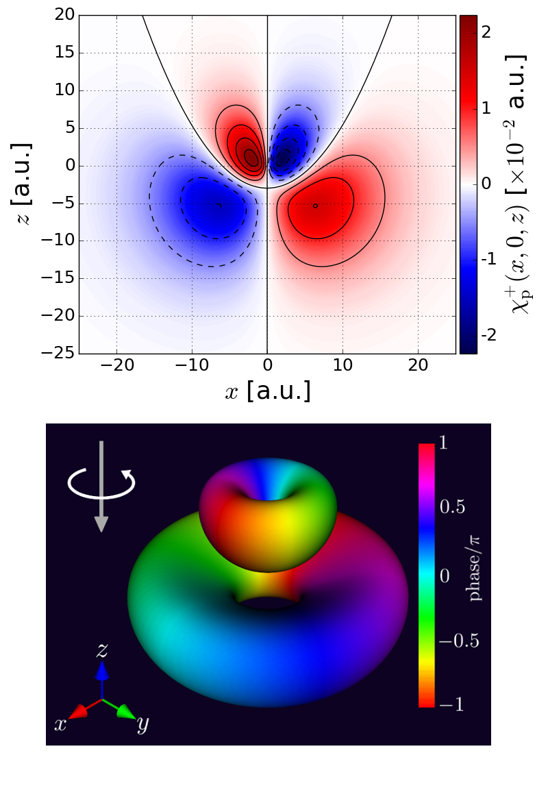
Figure 1: Top: contour map of $\chi_{\mathrm{p}}^{+}\left(\vec{r}\right)$ [Eq. (1)] on the $y=0$ plane, where it only takes real values. Dashed (solid) lines indicate negative (zero or positive) contours. Bottom: isosurface $\left|\chi_{\mathrm{p}}^{+}\left(\vec{r}\right)\right|=0.01\,\mathrm{a.u.}$ colored according to the phase. The chiral symbol on the upper left corner indicates the polarization of the density (vertical arrow) and the probability current in the azimuthal direction (curved arrow).

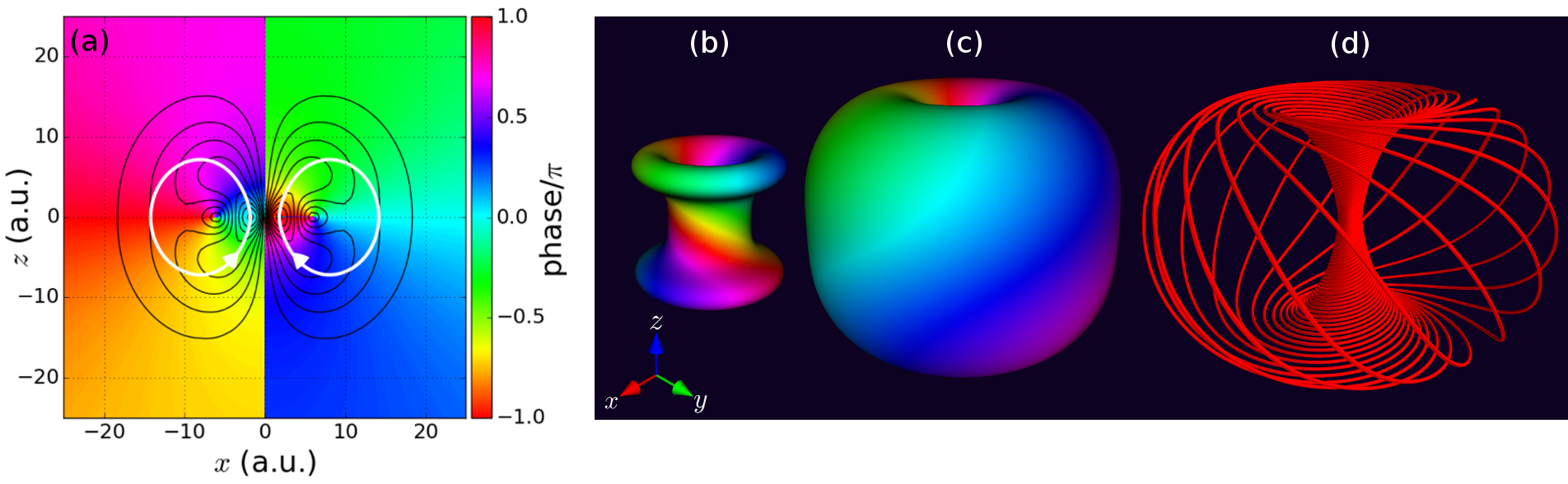
Figure 2: (a) Cut of $\chi_{\mathrm{c}}^{+}\left(\vec{r}\right)$ [Eq. (2)] on the $y=0$ plane. The black lines indicate the contours of $\left|\chi_{\mathrm{c}}^{+}\left(\vec{r}\right)\right|$ while the colors indicate its phase. The white arrows indicate the direction of the component of the probability current in the $y=0$ plane. (b) Isosurfaces $\left|\chi_{\mathrm{c}}^{+}\left(\vec{r}\right)\right|=0.011\,\mathrm{a.u.}$ and (c) $\left|\chi_{\mathrm{c}}^{+}\left(\vec{r}\right)\right|=0.005\,\mathrm{a.u.}$ colored according to the phase. (d) Trajectory followed by an element of the probability fluid $\left|\chi_{\mathrm{c}}^{+}\left(\vec{r}\right)\right|^{2}$. The rotation around the $z$ axis is counterclockwise. The radial distance in this specific trajectory varies between 1 and 18.5 a.u.

The second type ($\mathrm{c}$-type) is given by

$$\left|\chi_{\mathrm{c}}^{\pm}\right\rangle=\frac{1}{\sqrt{2}}\left(\left|3p_{\pm 1}\right\rangle+\mathrm{i}\left|3d_{\pm 1}\right\rangle\right),$$ (2)

which differs from $\left|\chi_{\mathrm{p}}\right\rangle$ only in the imaginary coefficient in front of $\left|3d_{\pm 1}\right\rangle$. At first sight, since $\langle\vec{r}|3p_{\pm 1}\rangle$ and $\langle\vec{r}|3d_{\pm 1}\rangle$ are complex functions, one would not expect important differences between $\mathrm{p}$ and $\mathrm{c}$ states, however, as shown in Fig. 2, the $\mathrm{p}$ and $\mathrm{c}$ states are qualitatively different. We can see that instead of the polarization along $z$, there is probability current circulating around a nodal circle of radius $6\,\mathrm{a.u.}$ in the $z=0$ plane, as indicated by the two circular arrows in Fig. 2 (a). Analogously to the $\mathrm{p}$ states, where the polarization of the probability density is determined by the relative sign between $\left|3p_{\pm 1}\right\rangle$ and $\left|3d_{\pm 1}\right\rangle$, in the $\mathrm{c}$ states the direction of the probability current is determined by the relative sign between $\left|3p_{\pm 1}\right\rangle$ and $\mathrm{i}\left|3d_{\pm 1}\right\rangle$. This vertical current combined with the horizontal current in the azimuthal direction due to $m=\pm 1$ leads to a chiral probability current (hence the $\mathrm{c}$ subscript), visualized in Fig. 2 (d) via the trajectory followed by an element of the probability fluid $\left|\chi_{\mathrm{c}}^{+}\right|^{2}$. This single trajectory (also known as a streamline in the context of fluids) clearly shows how, although pure helical motion of the electron is not compatible with a bound state, helical motion can still take place in a bound state via opposite helicities in the inner and outer regions. As can be inferred from the cut of $\chi_{\mathrm{c}}^{+}\left(\vec{r}\right)$ in the $y=0$ plane [Fig. 2 (a)], trajectories passing far from the nodal circle, like that shown in Fig. 2 (d), circulate faster in the azimuthal direction than around the nodal circle while those close to the nodal circle have the opposite behavior and look like the wire in a toroidal solenoid. Interestingly, a probability current with the same topology was found in Ref. Hegstrom et al. (1988) when analyzing the effect of the (chiral) weak interaction on the hydrogenic state $2p_{1/2}$.

So far we have only considered wave functions with achiral probability densities whose chirality relies on non-zero probability currents. The helical phase structure of $\chi_{\mathrm{c}}^{\pm}\left(\vec{r}\right)$ [see Figs. 2 (b) and (c)] suggests that we can construct a wave function $\chi_{\rho}^{\pm}\left(\vec{r}\right)$ with chiral probability density (hence the subscript $\rho$) by taking the real part of $\chi_{\mathrm{c}}^{\pm}\left(\vec{r}\right)$, i.e.

$$\left|\chi_{\rho}^{\pm}\right\rangle = \frac{1}{\sqrt{2}}\left(\left|\chi_{\mathrm{c}}^{\pm}\right\rangle+\mathrm{c.c.}\right)$$

$$= \frac{1}{2}\left(\left|3p_{\pm 1}\right\rangle+\mathrm{i}\left|3d_{\pm 1}\right\rangle-\left|3p_{\mp 1}\right\rangle+\mathrm{i}\left|3d_{\mp 1}\right\rangle\right)$$

$$= \frac{1}{\sqrt{2}}\left[\mp\left|3p_{x}\right\rangle+\left|3d_{yz}\right\rangle\right].$$

It turns out that this wave function is not chiral. Nevertheless, increasing the $l$ values by one results in the wave function we are looking for. The third type ($\rho$-type) of chiral wave function is given by

$$\left|\chi_{\rho\left(421\right)}^{\pm}\right\rangle = \frac{1}{\sqrt{2}}\left(\left|\chi_{\mathrm{c}\left(421\right)}^{\pm}\right\rangle+\mathrm{c.c.}\right)$$

$$= \frac{1}{2}(\left|4d_{\pm 1}\right\rangle+\mathrm{i}\left|4f_{\pm 1}\right\rangle-\left|4d_{\mp 1}\right\rangle+\mathrm{i}\left|4f_{\mp 1}\right\rangle)$$

$$= \frac{1}{\sqrt{2}}\left(\mp\left|4d_{xz}\right\rangle+\left|4f_{yz^{2}}\right\rangle\right)$$

Figure 3: Isosurfaces $\chi_{\mathrm{\rho}\left(421\right)}^{+}\left(\vec{r}\right)=\pm 0.001\,\mathrm{a.u.}$ (left) and $\chi_{\mathrm{\rho}\left(421\right)}^{+}\left(\vec{r}\right)=\pm 0.008\,\mathrm{a.u.}$ (right) [Eq. (II)] viewed along the $x$ (top) and $z$ (bottom) axes.

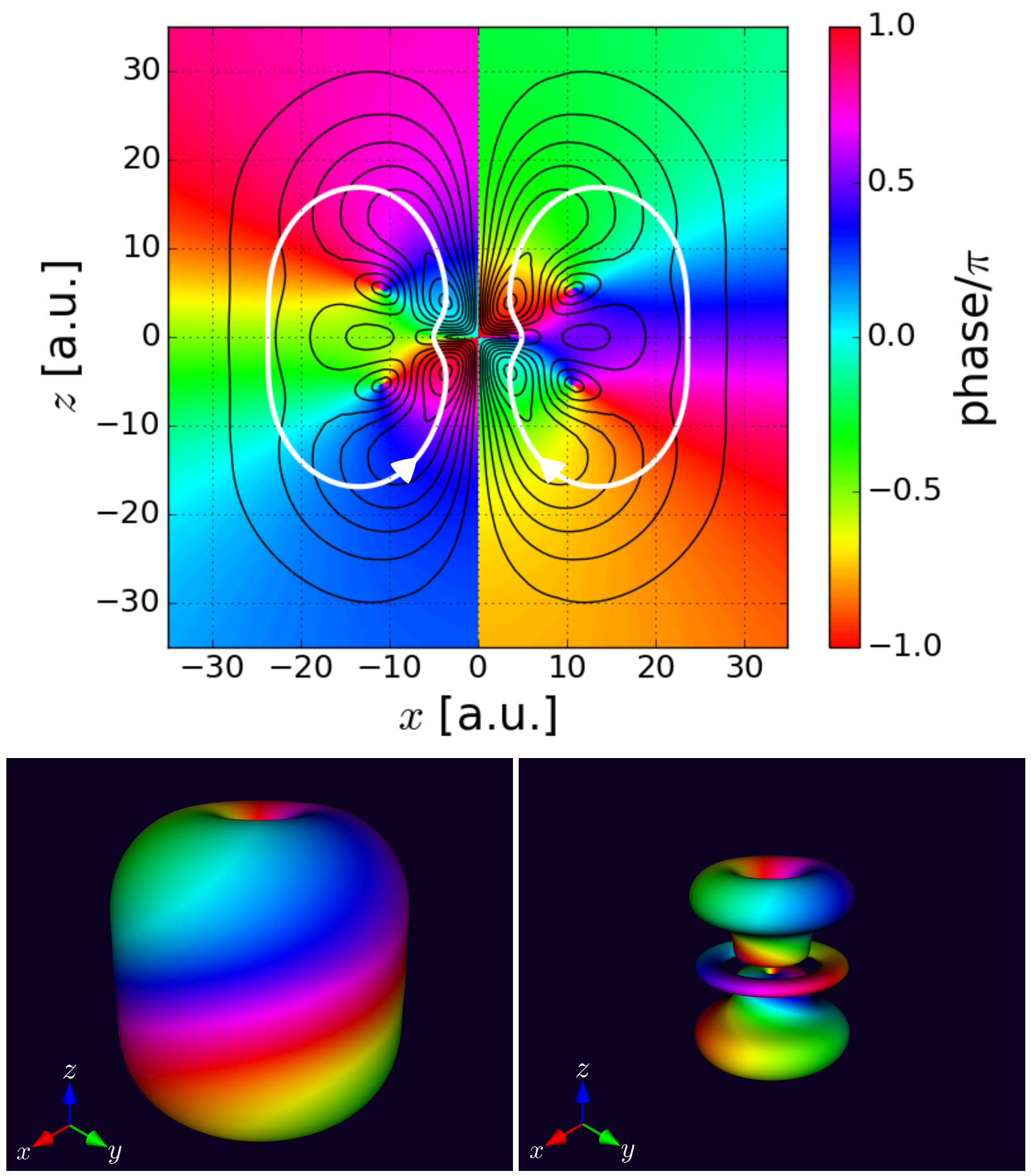
Figure 4: Top: cut of $\chi_{\mathrm{c}\left(421\right)}^{+}\left(\vec{r}\right)$ [Eq. (6)] on the $y=0$ plane. The black lines indicate the contours of $|\chi_{\mathrm{c}\left(421\right)}^{+}\left(\vec{r}\right)|$ while the colors indicate its phase. The white arrows indicate the direction of the component of the probability current in the $y=0$ plane. Bottom: isosurfaces $|\chi_{\mathrm{c}\left(421\right)}^{+}\left(\vec{r}\right)|=0.001\,\mathrm{a.u.}$ (left) and $|\chi_{\mathrm{c}\left(421\right)}^{+}\left(\vec{r}\right)|=0.004\,\mathrm{a.u.}$ (right) colored according to the phase.

and is shown in Fig. 3 for $m=1$. In Eq. (II) we introduced the notation

$$\left|\chi_{\mathrm{p}\left(nl\left|m\right|\right)}^{\pm}\right\rangle\equiv\frac{1}{\sqrt{2}}(\left|n,l,\pm\left|m\right|\right\rangle+\left|n,l+1,\pm\left|m\right|\right\rangle)$$ (5)

$$\left|\chi_{\mathrm{c}\left(nl\left|m\right|\right)}^{\pm}\right\rangle\equiv\frac{1}{\sqrt{2}}(\left|n,l,\pm\left|m\right|\right\rangle+\mathrm{i}\left|n,l+1,\pm\left|m\right|\right\rangle)$$ (6)

$$\left|\chi_{\rho\left(nl\left|m\right|\right)}^{\pm}\right\rangle\equiv\frac{1}{\sqrt{2}}\left(\left|\chi_{\mathrm{c},\left(nl\left|m\right|\right)}^{\pm}\right\rangle+\mathrm{c.c.}\right),\,l\geq 2,$$ (7)

which includes straightforward modifications to the simplest cases in Eqs. (1), (2), and (II) that we have already considered. Figure 4 shows $\chi_{\mathrm{c}\left(421\right)}^{+}\left(\vec{r}\right)$, which was used in Eq. (II), and Figs. 5 and 6 the $m=2$ variations $\chi_{\mathrm{c}\left(422\right)}^{+}\left(\vec{r}\right)$ and $\chi_{\rho\left(422\right)}^{+}\left(\vec{r}\right)=\left(\langle\vec{r}|4d_{x^{2}-y^{2}}\rangle-\langle\vec{r}|4f_{xyz}\rangle\right)/\sqrt{2}$ , which will be used for the analysis of PECD in the next subsection. As can be seen in Figs. 3 and 6, like the $\mathrm{c}$ states, the $\rho$ states also have helical structures of opposite handedness in the inner and outer regions.

The $\rho$ states are particularly meaningful because they mimic the electronic ground state of an actual chiral molecule in the sense that unlike the $\mathrm{p}$ and the $\mathrm{c}$ states, their chirality is completely encoded in the probability density and does not rely on probability currents. The decomposition of $\rho$ states into $\mathrm{c}$ states is the chiral analogue of the decomposition of a standing wave into two waves traveling in opposite directions, and, as we shall see in the next subsection, it will provide the corresponding advantages.

Finally, note that according to Barron’s definition of true and false chirality Barron (1986), the p states display false chirality because a time reversal yields the opposite enantiomer, while the c and $\rho$ states display true chirality because a time-reversal yields the same enantiomer.

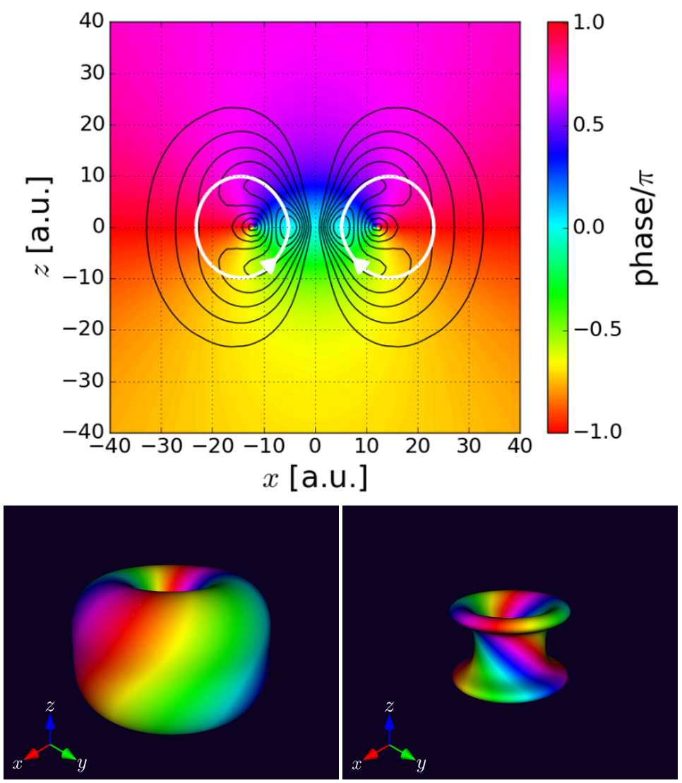
Figure 5: Top: cut of $\chi_{\mathrm{c}\left(422\right)}^{+}\left(\vec{r}\right)$ [Eq. (6)] on the $y=0$ plane. The white arrows indicate the direction of the component of the probability current in the $y=0$ plane. Bottom: isosurfaces $|\chi_{\mathrm{c}\left(422\right)}^{+}\left(\vec{r}\right)|=0.003\,\mathrm{a.u.}$ (left) and $|\chi_{\mathrm{c}\left(422\right)}^{+}\left(\vec{r}\right)|=0.005\,\mathrm{a.u.}$ (right) colored according to the phase.

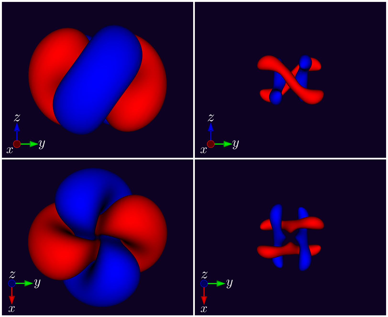
Figure 6: Isosurfaces $\chi_{\mathrm{\rho}\left(422\right)}^{+}\left(\vec{r}\right)=\pm 0.001\,\mathrm{a.u.}$ (left) and $\chi_{\mathrm{\rho}\left(422\right)}^{+}\left(\vec{r}\right)=\pm 0.006\,\mathrm{a.u.}$ (right) [Eq. (7)] viewed along the $x$ (top) and $z$ (bottom) axes.

III The sign of the forward-backward asymmetry in aligned chiral hydrogen

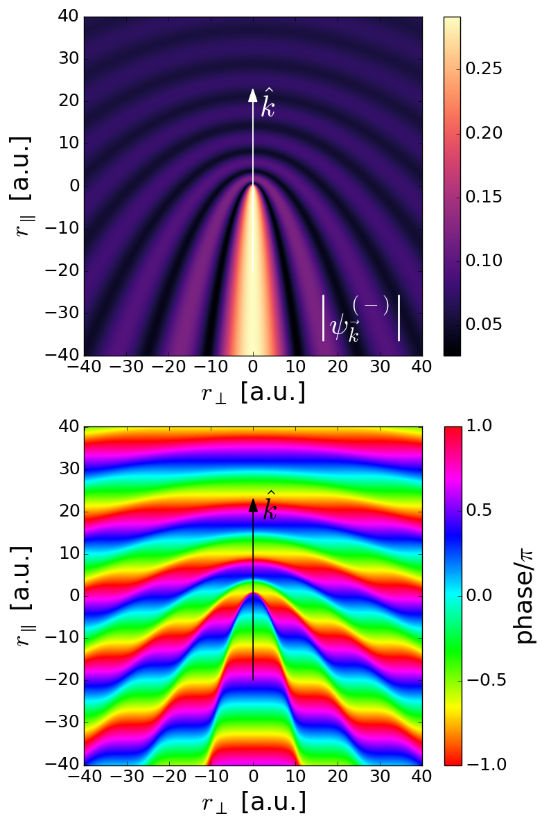
Figure 7: Absolute value (top) and phase (bottom) of the scattering wave function $\psi_{\vec{k}}^{\left(-\right)}$ evaluated in a plane containing $\vec{k}$ for $k=0.3\,\mathrm{a.u.}$ $r_{\parallel}$ and $r_{\perp}$ are the coordinates parallel and perpendicular to $\vec{k}$, respectively.

Now we consider photoionization from the chiral bound states just introduced via circularly polarized light. For this, we require the scattering wave function $\psi_{\vec{k}}^{\left(-\right)}$. In the case of hydrogen, this wave function is known analytically Hans A. Bethe and Edwin Salpeter (1957). $\psi_{\vec{k}}^{\left(-\right)}\left(\vec{r}\right)$ has cylindrical symmetry with respect to $\vec{k}$ and is shown in Fig. 7 for $k=0.3\,\mathrm{a.u.}$ in a plane containing $\vec{k}$. Since only hydrogenic functions are involved, the calculation of the transition dipole matrix element $\langle\psi_{\vec{k}}^{\left(-\right)}|\vec{r}\left|\chi\right\rangle$ can be carried out analytically. The angular integrals reduce to 3-j symbols Brink and Satchler (1968) and the radial integrals can be calculated using the method of contour integration described in Hans A. Bethe and Edwin Salpeter (1957).

The angle-integrated photoelectron current $\vec{j}\left(k\right)$ can be extracted from the angular and energy dependent ionization probability $W_{\sigma}\equiv|\langle\psi_{\vec{k}}^{\left(-\right)}|\vec{r}\cdot\tilde{\vec{\mathcal{E}}}_{\sigma}\left|\chi\right\rangle|^{2}$, where $\tilde{\vec{\mathcal{E}}}$ is the Fourier transform of the field and $\sigma=\pm 1$ indicates the rotation direction of the field (see also Ref. Ordonez and Smirnova (2018b)). First we do a partial wave expansion of $W_{\sigma}$,

$$W_{\sigma}(\vec{k})=\sum_{l,m}b_{l,m}\left(k,\sigma\right)Y_{l}^{m}(\hat{k}),$$ (8)

and then we replace it in the expression for the $z$ component of the angle-integrated photoelectron current,

$$j_{z}\left(k,\sigma\right)=\int\mathrm{d}\Omega_{k}W_{\sigma}(\vec{k})k_{z}=\sqrt{\frac{4\pi}{3}}kb_{1,0}\left(k,\sigma\right).$$ (9)

For normalization purposes, one can also consider the radial component of the angle-integrated photoelectron current, which yields

$$j_{r}\left(k,\sigma\right)=\int\mathrm{d}\Omega_{k}W_{\sigma}(\vec{k})k=\sqrt{4\pi}kb_{0,0}\left(k,\sigma\right)$$ (10)

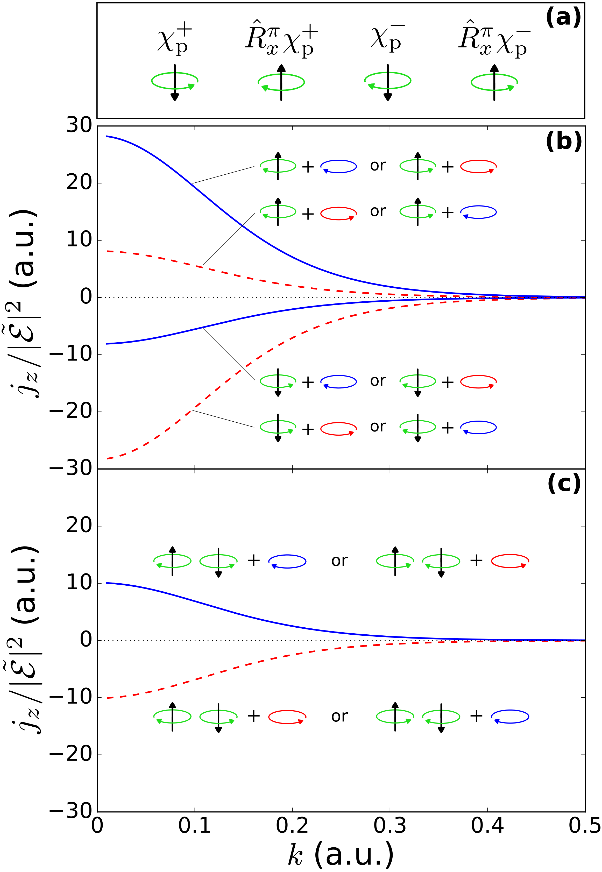
Figure 8: Photoelectron current along $z$ as a function of photoelectron momentum resulting from photoionization of a p-type chiral state [see Eq. (5)] via light circularly polarized in the $xy$ plane. (a) Diagrams indicating the electronic polarization (vertical arrow) and the electronic current (circular arrow) in the p-type chiral states for two opposite enantiomers and two opposite orientations. $\hat{R}_{x}^{\pi}$ is the operator that rotates the wave function by $\pi$ radians around the $x$ axis. (b) Photoelectron current [Eq. (9)] for different enantiomer, orientation, and light polarization combinations. The enantiomer and its orientation is indicated by the diagrams explained in (a), and the light polarization is indicated by the circular arrows after the plus signs. Note that the sign of $j_{z}$ is determined by the direction of the electronic polarization and that the magnitude of $j_{z}$ is determined by the relative direction between the electronic current and the light polarization. (c) Photoelectron current averaged over two opposite orientations (equivalent to the aligned case) for different combinations of enantiomer and light polarization. There is no cancellation of the asymmetry because for one orientation the bound electron co-rotates with the field, while for the opposite orientation it counter-rotates. The calculations shown are for the states $\chi_{\mathrm{p}\left(311\right)}^{\pm}$ but the conclusions are valid for any $\chi_{\mathrm{p}\left(nlm\right)}^{\pm}$ state.

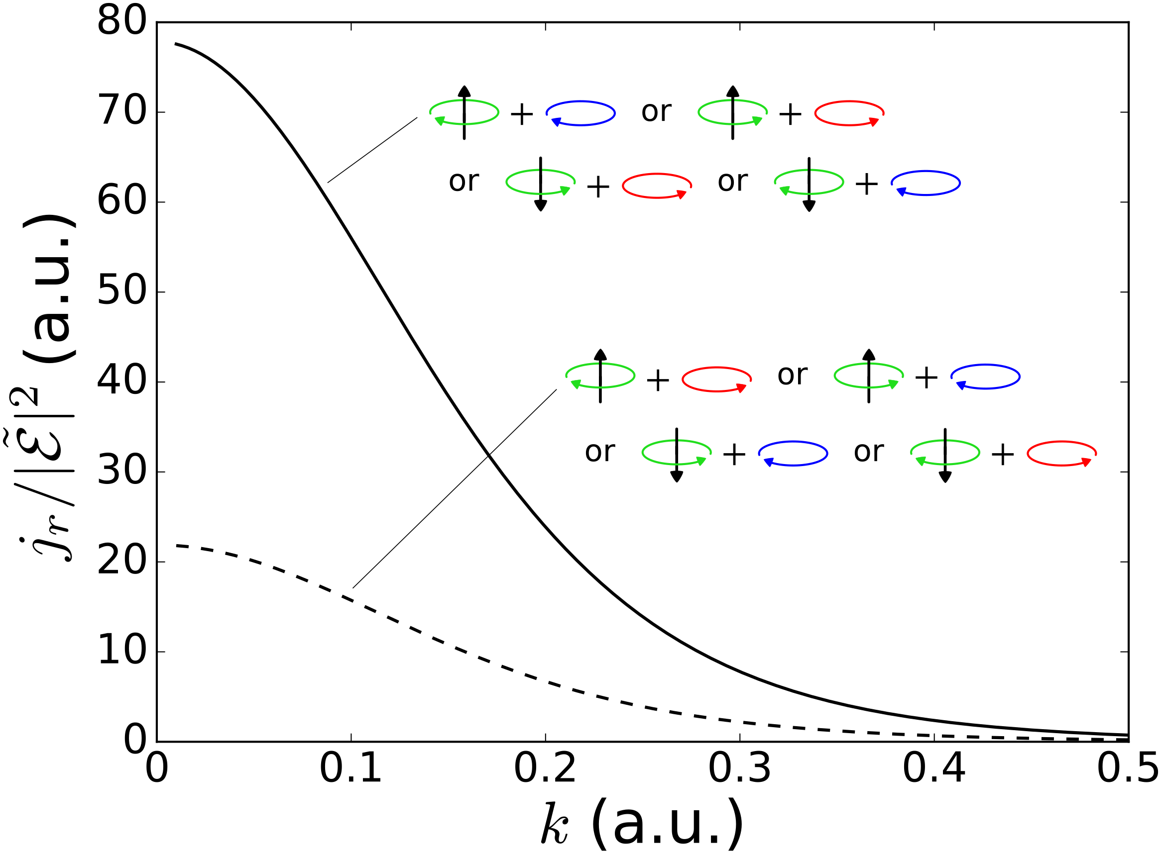
Figure 9: Total photoelectron current resulting from photoionization of a p-type chiral state [see Eq. (5)] via light circularly polarized in the $xy$ plane for different enantiomer, orientation, and light polarization combinations. Diagrams are explained in Fig. 8 (a). Only the relative direction between the bound electronic current and the rotating electric field determines $j_{r}$. The calculations shown are for the states $\chi_{\mathrm{p}\left(311\right)}^{\pm}$ but the conclusions are valid for any $\chi_{\mathrm{p}\left(nlm\right)}^{\pm}$ state.

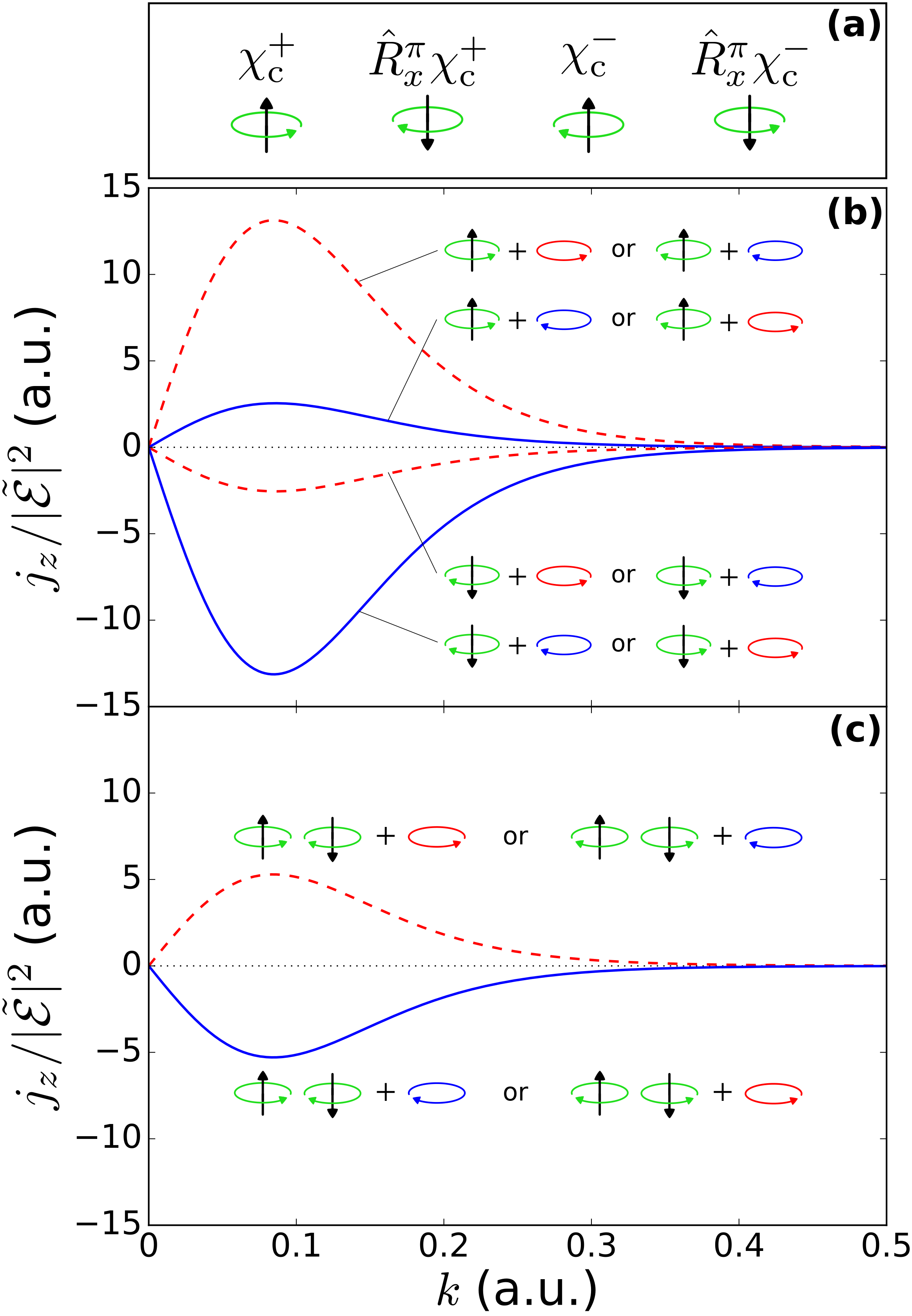
Figure 10: Same as Fig. 8 but for the c-type chiral states [see Eq. (6)]. The role played by the electronic polarization in the p-type states is replaced by the vertical component of the probability current in the inner region in the c-type states. The results in (c) are also valid for photoionization from $\rho$-type chiral states (see text). The calculations shown are for the states $\chi_{\mathrm{c}\left(422\right)}^{\pm}$ but the conclusions are valid for any $\chi_{\mathrm{c}\left(nlm\right)}^{\pm}$ state.

Figures 8 (a), 8 (b), and 9 show $j_{z}\left(k,\sigma\right)$ and $j_{r}\left(k,\sigma\right)$ for the case of photoionization from the initial states $|\chi_{\mathrm{p}\left(311\right)}^{\pm}\rangle$ [see Eq. (1)] with their $z$ molecular axis perpendicular to the plane of polarization of the ionizing light. We can clearly see two propensity rules that also hold for any other $|\chi_{\mathrm{p}\left(nlm\right)}^{\pm}\rangle$ state: (i) the direction of $j_{z}$ is determined by the electronic polarization direction of $\chi_{\mathrm{p}\left(nlm\right)}^{\pm}(\vec{r})$ and (ii) the magnitudes of $j_{r}$ and $j_{z}$ are bigger when the bound electron rotates in the same direction as the electric field in comparison to when they rotate in opposite directions. The first propensity rule is a consequence of the non-plane-wave nature of the continuum wave function $\psi_{\vec{k}}^{\left(-\right)}\left(\vec{r}\right)$ (see Fig. 7), which resembles a bound polarized structure and leads to improved overlap between $\psi_{\vec{k}}\left(\vec{r}\right)$ and $\chi_{\mathrm{p}\left(nlm\right)}^{\pm}\left(\vec{r}\right)$ in the dipole matrix element when the direction of electronic polarization and the direction of the photoelectron coincide as compared to when they are opposite to each other. The polarized structure of $\psi_{\vec{k}}^{\left(-\right)}\left(\vec{r}\right)$ decays monotonously with increasing $k$ and vanishes in the plane-wave limit, which explains the monotonous decay of $j_{z}\left(k\right)$. The second propensity rule is well known in the 1-photon-absorption atomic case Hans A. Bethe and Edwin Salpeter (1957). This rule changes with the ionization regime Ilchen et al. (2017b); Barth and Smirnova (2011, 2013).

In the aligned case, thanks to the vector nature of the photoelectron current, it is enough to consider only two opposite orientations (see Sec. III in our companion paper Ordonez and Smirnova (2018a)). In view of the first propensity rule we have that for the two opposite orientations the polarization will point in opposite directions and therefore $j_{z}$ will have opposite signs. However, since for opposite orientations the bound electron current also rotates in opposite directions while the light polarization remains fixed, the magnitude of $j_{z}$ will be different for each orientation, thus avoiding a complete cancellation of the asymmetry. Furthermore, as can be seen in Fig. 8 (c), the sign of the orientation-averaged $j_{z}$ will be that of the orientation where the electron co-rotates with the electric field of the light. That is, the propensity rule for the aligned case is that the total photoelectron current $\vec{j}=j_{z}\hat{z}$ will point in the direction of electronic polarization associated to the orientation where the bound electronic current co-rotates with the ionizing electric field.

A similar analysis can be carried out for the case of photoionization from the initial states $|\chi_{\mathrm{c}\left(nlm\right)}^{\pm}\rangle$, shown in Fig. 10 for the specific case where $\left(nlm\right)=(422)$ but valid for any other values of $\left(nlm\right)$. The only difference is that in this case the role which was played by the electronic polarization in the p-type states is now played by the vertical component of the electronic current in the inner region. Like before, this result can be understood by considering the overlap between the initial and final states. The polarized structure of the continuum state determines the region contributing more to the dipole matrix element (see $|\psi_{\vec{k}}^{\left(-\right)}(\vec{r})|$ in Fig. 7) and the relative direction between the probability currents in the initial and final states in this region determines the amount of overlap. When the direction of the probability current of $\chi_{\mathrm{c}\left(nlm\right)}^{+}\left(\vec{r}\right)$ in the inner region (which is where $|\psi_{\vec{k}}^{\left(-\right)}\left(\vec{r}\right)|$ is greatest) is parallel to the direction of $\vec{k}$ the overlap is maximized. Therefore, the propensity rule in this case is that the sign of $j_{z}$ is positive/negative when the vertical component of the electronic current in the inner region points up/down. The non-monotonous behavior of $j_{z}$ as a function of $k$ obeys the fact that this propensity rule not only relies on the polarized nature of $|\psi_{\vec{k}}^{\left(-\right)}\left(\vec{r}\right)|$, but also on the direction of the continuum probability current, therefore, for $k\rightarrow 0$, although the density of the continuum state is maximally polarized, its probability current tends to zero, rendering it unable to distinguish the direction of the probability current of the bound state, which is the feature responsible for the FBA in the first place. At an intermediate photoelectron momentum $k\approx 0.1\,\mathrm{a.u.}$ the probability current of the continuum state matches that of the bound state and the sensitivity of the continuum state to the direction of the probability current of the bound state is optimal. For larger values of $k$, the match worsens and the continuum also becomes less and less polarized leading to a monotonic decay of the FBA. The other propensity rule regarding the relative rotation of the bound current and the electric field remains the same and, again, the contributions from opposite orientations to $j_{z}$ do not completely cancel each other.

Finally, in the case where the photoionization takes place from the states $|\chi_{\rho\left(nlm\right)}^{\pm}\rangle$ [see Eq. (7)], there is neither any probability current nor any net polarization that we can rely on. Furthermore, one can see from Figs. 3 and 6 that the wave function $\chi_{\rho\left(nlm\right)}^{\pm}\left(\vec{r}\right)$ is invariant with respect to rotations by $\pi$ either around the $x$ or the $y$ axis, so that $j_{z}$ is the same for both orientations. Thus the situation appears to be quite different from what we had for the states $|\chi_{\mathrm{p}\left(nlm\right)}^{\pm}\rangle$ and $|\chi_{\mathrm{c}\left(nlm\right)}^{\pm}\rangle$. However, we know that the chiral probability density of $|\chi_{\rho\left(nlm\right)}^{\pm}\rangle$ is the result of the superposition of the chiral currents from $|\chi_{\mathrm{c}\left(nlm\right)}^{\pm}\rangle$ and its complex conjugate. These two chiral currents flow in opposite directions therefore, when we subject $|\chi_{\rho\left(nlm\right)}^{\pm}\rangle$ to a field circularly polarized in the $xy$ plane, one part of $|\chi_{\rho\left(nlm\right)}^{\pm}\rangle$ will be counter-rotating and the other part will be co-rotating with the field. One part will have an upwards vertical current in the inner region and the other will have a downwards vertical current in the inner region. Thus the situation for a single orientation of $|\chi_{\rho\left(nlm\right)}^{\pm}\rangle$ is very similar to what we had before when we considered two opposite orientations of $|\chi_{\mathrm{c}\left(nlm\right)}^{\pm}\rangle$. In fact, as shown in Appendix VII.2, both situations are exactly equivalent in the case of an isotropic continuum like that of hydrogen. That is, the $z$ component of the photoelectron current resulting from photoionization from the state $|\chi_{\rho\left(nlm\right)}^{\pm}\rangle$ is equal to that obtained from $|\chi_{\mathrm{c}\left(nlm\right)}^{\pm}\rangle$ after averaging over two opposite orientations. The results plotted in Fig. 10 (c) are not only those obtained for $|\chi_{\mathrm{c}\left(422\right)}^{\pm}\rangle$, but also those obtained for $|\chi_{\rho\left(422\right)}^{\pm}\rangle$. This shows that although the $\rho$-type states do not display any bound probability current, we can still make sense of the sign of the FBA displayed by their photoelectron angular distribution through their decomposition into $c$-type states.

An example of how to use these propensity rules for the less symmetric cases where the orientation of the molecular $z$ axis is in the plane of the light polarization is given in Appendix VII.3.

IV Extensions of the model

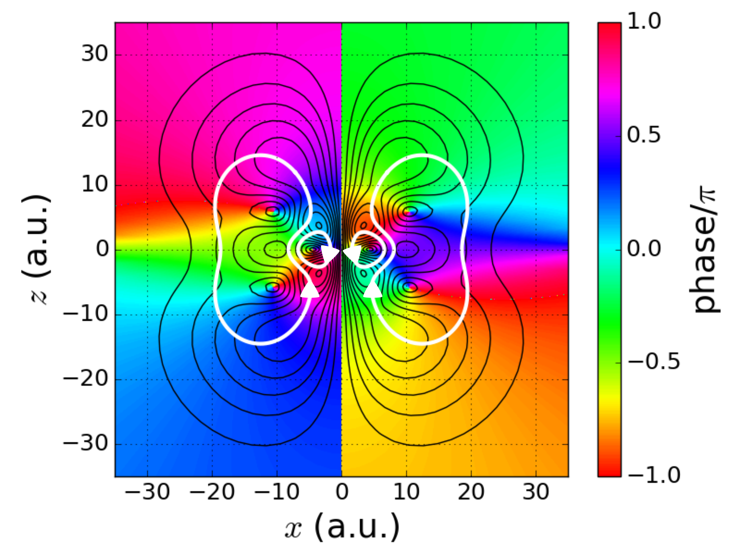
Figure 11: Cut of $\chi_{\mathrm{c}}^{+-}\left(\vec{r}\right)$ [Eq. (11)] on the $y=0$ plane. The white arrows indicate the direction of the component of the probability current in the $y=0$ plane. The extra loops in the innermost region (cf. Fig. 4) allow for an extra degree of handedness. One handedness is associated to the big loops $(+)$ and the other to the small loops $(-)$.

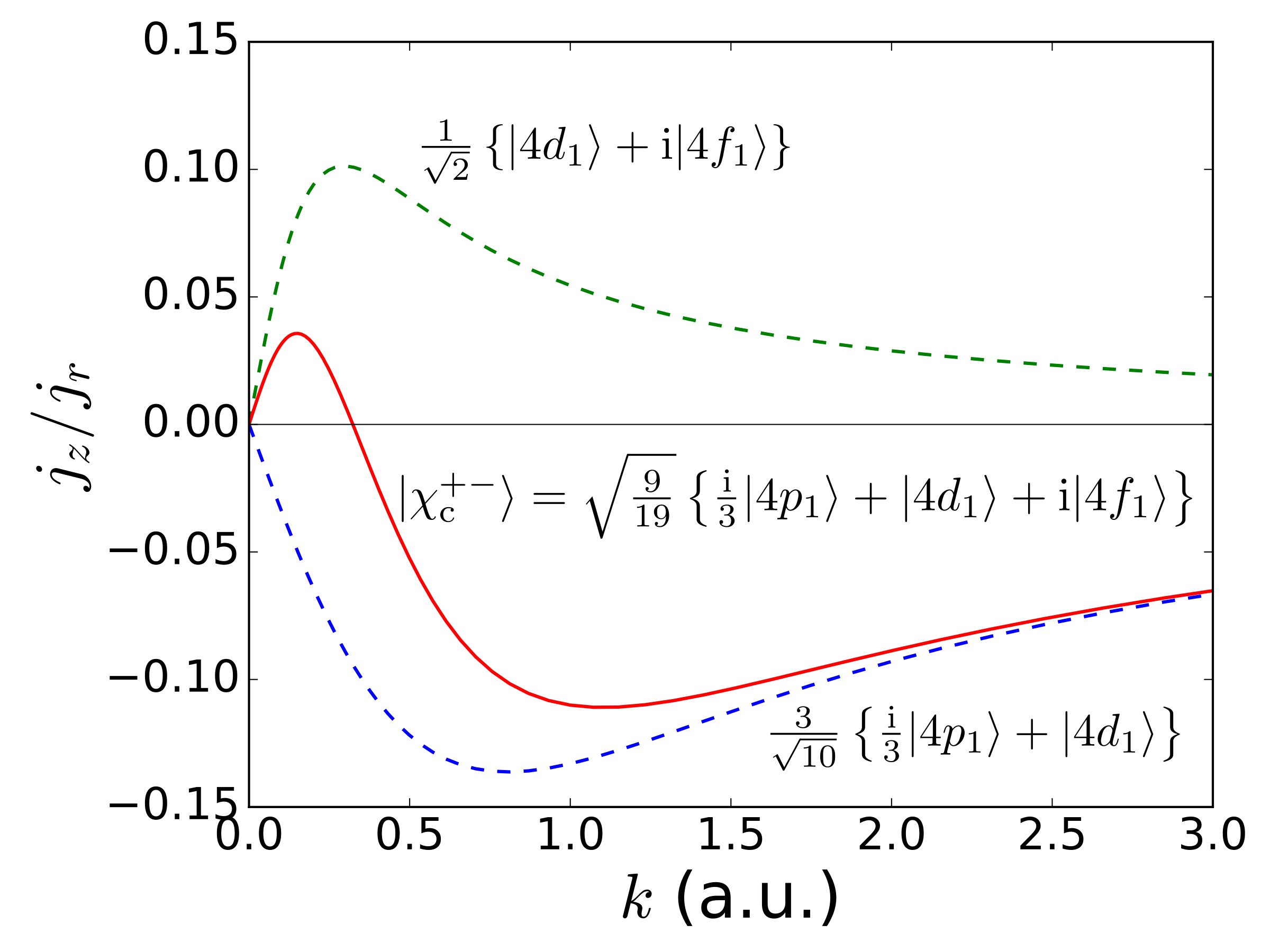
Figure 12: Normalized photoelectron current [Eqs. (9) and (10)] as a function of photoelectron momentum resulting from photoionization of the initial state $|\chi_{\mathrm{c}}^{+-}\rangle$ in Eq. (11) (solid red line) via light left circularly polarized (rotating counter-clockwise as viewed from the $+z$ direction) and alignment perpendicular to the light polarization plane. The FBA changes sign as a function of photoelectron energy $k^{2}/2$ reflecting the ambivalent handedness of $|\chi_{\mathrm{c}}^{+-}\rangle$ (see Fig. 11). The dashed lines show the corresponding currents for the ‘single-handed’ states that make up $|\chi_{\mathrm{c}}^{+-}\rangle$.

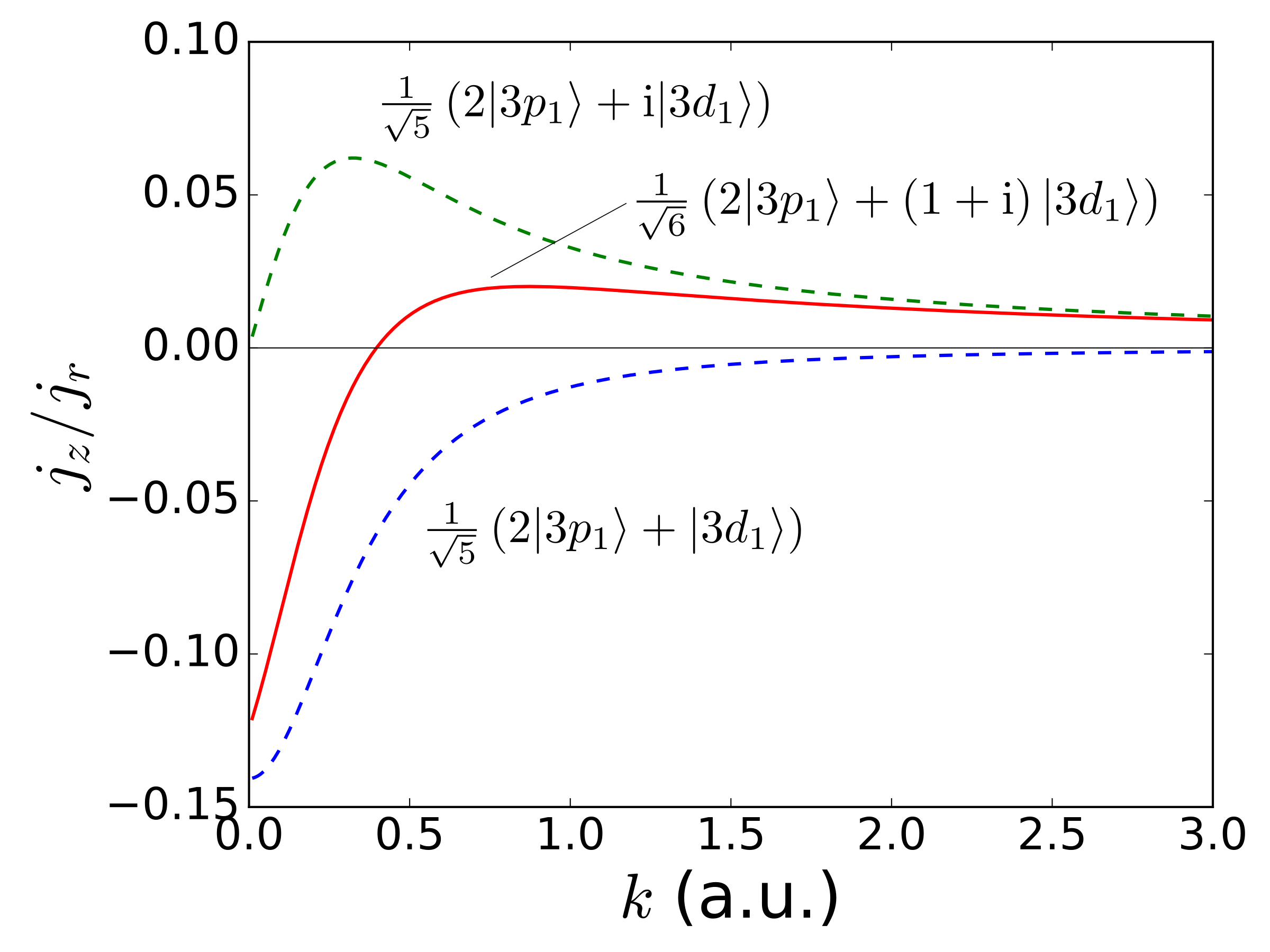
Figure 13: Normalized photoelectron current [Eqs. (9) and (10)] as a function of photoelectron momentum resulting from photoionization of the initial state $|\chi_{\mathrm{p}(311)}^{+}\rangle+|\chi_{\mathrm{c}(311)}^{+}\rangle$ (solid red line) via light left circularly polarized (rotating counter-clockwise as viewed from the $+z$ direction) and alignment perpendicular to the light polarization plane. The FBA changes sign as a function of photoelectron energy $k^{2}/2$ reflecting the p-like (lower dashed line) and c-like character (upper dashed line) at lower and higher photoelectron energies, respectively.

So far we have restricted our discussion to bound wave functions involving only two different consecutive angular momenta $l$ with a specific phase between them of $0$, $\pi$ (p-type states), or $\pm\pi/2$ radians (c-type states). To get an idea of how increasing the complexity of the bound wave function may affect the FBA and the corresponding propensity rules we will consider what happens when we introduce either a third $l$ component or an arbitrary phase shift between the two $l$ components.

A third $l$ component simply introduces the possibility of having a single wave function with more than one handedness (like a helix made of a tighter bound helix) and therefore a FBA which may change sign as a function of energy, a feature seen in actual molecules but absent in the simplest possible chiral wave functions we have presented. Consider for example the c-type wave function with three $l$ values given by

$$|\chi_{\mathrm{c}}^{+-}\rangle=\sqrt{\frac{9}{19}}\left\{\frac{\mathrm{i}}{3}|4p_{1}\rangle+|4d_{1}\rangle+\mathrm{i}|4f_{1}\rangle\right\},$$ (11)

which is a superposition of $|4p_{1}\rangle$ and the state $|\chi_{\mathrm{c}(421)}\rangle$ [see Eq. (6)]. A plot of this wave function on the plane $y=0$ is shown in Fig. 11 (compare with Fig. 4). Unlike the states $|\chi_{\mathrm{c}(nml)}^{\pm}\rangle$, where the chiral current displays a single handedness, the state $|\chi_{\mathrm{c}}^{+-}\rangle$ displays two possible handedness, one associated with the big current loops and the other one associated with the small current loops in Fig. 11. Since the two chiral currents are confined to regions of different sizes, high (low) energy photoelectrons will probe more efficiently the chirality associated to the smaller (bigger) loops, and therefore one may observe a change of sign in the FBA as the photoelectron energy is increased. Figure 12 shows how each chiral component contributes to the total FBA. An analogous behavior is observed for the case of p-type states.

Clearly, closed current loops like those shown in Fig. 11 can only occur around a zero of the wave function, and the emergence of the small loops in Fig. 11 is associated with the emergence of a zero at $r\approx 4.4$ a.u., $\theta=\pi/2$. At the same time, the change of sign of the FBA is linked to the existence of the small loops, which suggests an interesting link between the topology of the wave function (zeros and currents around them) and the zeros of the FBA as a function of photoelectron energy. Further investigation of this point will be presented in a forthcoming publication.

Introduction of phases differing from zero or $\pi/2$ between consecutive $l$ components simply means that instead of having a pure p- or a pure c-type state we have a superposition of both. This can also lead to a FBA that changes sign as a function of energy because the behavior of the FBA as a function of energy is different for p and c states. For example, as shown in Fig. 13, a state $|\chi_{\mathrm{p}\left(311\right)}^{+}\rangle+|\chi_{\mathrm{c}\left(311\right)}^{+}\rangle$ displays a FBA which is negative at lower energies and positive at higher energies, i.e. it reflects the p character at lower energies and the c character at higher energies.

Although the concepts of polarization, current, and wave-function overlap, underlying the propensity rules are general, the assignment of specific propensity rules to chiral molecules can be impeded due to their considerably more complex electronic structure than the elementary chiral wave-functions introduced here. In the companion paper Ordonez and Smirnova (2018a) we develop an alternative route, bypassing the specific propensity rules and introducing a more general measure, which simply indicates the presence thereof. This measure –propensity field– controls the sign of forward-backward asymmetry in PECD.

V Conclusions

We have introduced three families of hydrogenic chiral wave functions that serve as basic tools for the analysis of electronic chiral effects. The chirality of these wave functions may be due either to a chiral density, a chiral probability current, or a combination of achiral density and achiral probability current.

We have used the chiral hydrogenic wave functions as a tool to explore the basic physical mechanisms underlying the chiral response in photoionization at the level of electrons. We have shown that two basic photoionization propensity rules determine the sign of the forward-backward asymmetry in photoelectron circular dichroism (PECD) in aligned molecules. One propensity rule selects the molecular orientations in which the electron and the electric field rotate in the same direction, and the other propensity rule determines whether the photoelectrons are emitted preferentially forwards or backwards. This simple picture illustrates that the propensity rules lie at the heart of photoelectron circular dichroism. In the companion paper Ordonez and Smirnova (2018a) we show how these ideas can be extended to the case of randomly oriented molecules, where another layer of effects of geometrical origin add to this simple picture.

VI Acknowledgements

A.F.O. and O.S. gratefully acknowledge the MEDEA project, which has received funding from the European Union’s Horizon 2020 research and innovation programme under the Marie Skłodowska-Curie grant agreement 641789. O.S. acknowledges support from the DFG SPP 1840 “Quantum Dynamics in Tailored Intense Fields” and the DFG grant SM 292/5-2.

VII Appendix

VII.1 Vanishing of the FBA for an orientation-independent continuum and an isotropically oriented ensemble

In this appendix we give a simple demonstration that an orientation-independent continuum yields a zero FBA when all molecular orientations are equally likely (see also Cherepkov (1982b)). Consider the lab-frame orientation-averaged photoelectron angular distribution

$$W_{\sigma}(\vec{k})=\int\mathrm{d}\lambda\left|\left\langle\psi_{\vec{k}}^{\left(-\right)}\middle|\hat{\epsilon}_{\sigma}\middle|\hat{D}(\lambda)\chi\right\rangle\right|^{2},$$ (12)

where $\hat{\epsilon}_{\sigma}\equiv\left(\hat{x}\pm\mathrm{i}\hat{y}\right)$, and $\hat{D}\left(\lambda\right)$ is the operator that rotates the bound wave function $\chi(\vec{r})$ by the Euler angles $\lambda\equiv\alpha\beta\gamma$. We assumed that the scattering wave function $\psi_{\vec{k}}^{\left(-\right)}(\vec{r})$ is independent of the molecular orientation $\lambda$ and therefore there is no need to rotate it. Here we consider rotations in the active sense, i.e. we always have the same frame of reference (the lab frame) and we rotate the functions. If we expand the bound wave function in spherical harmonics as

$$\chi\left(\vec{r}\right)=\sum_{l,m}u_{l,m}\left(r\right)Y_{l}^{m}\left(\hat{r}\right),$$ (13)

then the rotation operator $\hat{D}\left(\lambda\right)$ acts on $\chi\left(\vec{r}\right)$ through the Wigner D-matrices $D_{m^{\prime},m}^{\left(l\right)}\left(\lambda\right)$ according to

$$\hat{D}\left(\lambda\right)\chi\left(\vec{r}\right)=\sum_{l,m,m^{\prime}}D_{m^{\prime},m}^{\left(l\right)}\left(\lambda\right)u_{l,m}\left(r\right)Y_{l}^{m^{\prime}}\left(\hat{r}\right)=\sum_{l,m,m^{\prime}}D_{m^{\prime},m}^{\left(l\right)}\left(\lambda\right)\chi_{l,m,m^{\prime}}\left(\vec{r}\right).$$ (14)

Replacing this expansion in the expression for the photoelectron angular distribution we obtain

$$W_{\sigma}(\vec{k}) =\sum_{l_{1},m_{1},m_{1}^{\prime},l_{2},m_{2},m_{2}^{\prime}}\left[\int\mathrm{d}\lambda D_{m_{2}^{\prime},m_{2}}^{\left(l_{2}\right)*}\left(\lambda\right)D_{m_{1}^{\prime},m_{1}}^{\left(l_{1}\right)}\left(\lambda\right)\right]$$

$$\times\left\langle\psi_{\vec{k}}^{\left(-\right)}\middle|\hat{\epsilon}_{\sigma}\middle|\chi_{l_{2},m_{2},m_{2}^{\prime}}\right\rangle^{*}\left\langle\psi_{\vec{k}}^{\left(-\right)}\middle|\hat{\epsilon}_{\sigma}\middle|\chi_{l_{1},m_{1},m_{1}^{\prime}}\right\rangle.$$

$$=\sum_{l_{1},m_{1},m_{1}^{\prime}}\frac{8\pi^{2}}{2l_{1}+1}\left|\left\langle\psi_{\vec{k}}^{\left(-\right)}\middle|\hat{\epsilon}_{\sigma}\middle|\chi_{l_{1},m_{1},m_{1}^{\prime}}\right\rangle\right|^{2}$$ (15)

where we used the orthogonality relation for the Wigner D-matrices Brink and Satchler (1968). Now we expand the scattering wave function in spherical harmonics with respect to $\hat{k}$

$$\psi_{\vec{k}}^{\left(-\right)}\left(\vec{r}\right)=\sum_{l,m}\psi_{k,l,m}\left(\vec{r}\right)Y_{l}^{m*}(\hat{k}),$$ (16)

and replace it in the expression for the photoelectron angular distribution

$$W_{\sigma}(\vec{k}) =\sum_{l,m,l_{1},m_{1},m_{1}^{\prime}}\frac{8\pi^{2}}{2l_{1}+1}\left|\left\langle\psi_{k,l,m}\middle|\hat{\epsilon}_{\sigma}\middle|\chi_{l_{1},m_{1},m_{1}^{\prime}}\right\rangle Y_{l}^{m}(\hat{k})\right|^{2}$$

$$=\sum_{l,m}f_{\sigma,l,m}\left(k\right)\left|Y_{l}^{m}(\hat{k})\right|^{2}$$ (17)

where

$$f_{\sigma,l,m}(k)=\sum_{l_{1},m_{1},m_{1}^{\prime}}\frac{8\pi^{2}}{2l_{1}+1}\left|\left\langle\psi_{k,l,m}\middle|\hat{\epsilon}_{\sigma}\middle|\chi_{l_{1},m_{1},m_{1}^{\prime}}\right\rangle\right|^{2}.$$ (18)

Since $|Y_{l}^{m}(\hat{k})|^{2}$ is symmetric with respect to the $xy$ plane for every $l$ and $m$, Eq. (17) shows that $W_{\sigma}(\vec{k})$ is also symmetric with respect to the $xy$ plane, and thus exhibits no FBA, irregardless of the values of the coefficients $f_{\sigma,l,m}(k)$ which encode the information about the chiral bound state and the light polarization. Any deviation from an orientation-independent scattering wave function will introduce cross-terms in Eqs. (15) and (17), and therefore will open the possibility of non-zero FBA.

VII.2 Absence of m-coupling in the photoelectron current for isotropic continua

Consider the photoelectron angular distribution resulting from a single molecular orientation

$$W_{\sigma}(\vec{k})=\left|\left\langle\psi_{\vec{k}}^{\left(-\right)}\middle|\hat{\epsilon}_{\sigma}\middle|\chi\right\rangle\right|^{2},$$ (19)

where $\hat{\epsilon}_{\sigma}\equiv\left(\hat{x}\pm\mathrm{i}\hat{y}\right)$, $\chi$ is the bound wave function that has already been rotated by the Euler angles $\lambda\equiv\alpha\beta\gamma$, and the scattering wave function is molecular-orientation independent, i.e. it only depends on the relative direction between the position vector $\vec{r}$ and the photoelectron momentum $\vec{k}$. Both wave functions can be expanded as

$$\chi\left(\vec{r}\right)=\sum_{l,m}\chi_{l,m}\left(\vec{r}\right)$$ (20)

$$\psi_{\vec{k}}^{\left(-\right)}\left(\vec{r}\right)=\sum_{l,m}\psi_{l,m}\left(k,\vec{r}\right)Y_{l}^{m*}(\hat{k}),$$ (21)

where $\chi_{l,m}\left(\vec{r}\right)=u_{l,m}\left(r\right)Y_{l}^{m}\left(\hat{r}\right)$ and $\psi_{l,m}\left(k,\vec{r}\right)=v_{l,m}\left(k,r\right)Y_{l}^{m}\left(\hat{r}\right)$. Replacing these expansions in $W_{\sigma}(\vec{k})$ we get

$$W_{\sigma}(\vec{k})=\sum_{l_{1},m_{1},l_{2},m_{2},l_{1}^{\prime},l_{2}^{\prime}}\left\langle\psi_{l_{1}^{\prime},m_{1}+\sigma}\middle|\hat{\epsilon}_{\sigma}\middle|\chi_{l_{1},m_{1}}\right\rangle^{*}\left\langle\psi_{l_{2}^{\prime},m_{2}+\sigma}\middle|\hat{\epsilon}_{\sigma}\middle|\chi_{l_{2},m_{2}}\right\rangle\\ \times Y_{l_{1}^{\prime}}^{m_{1}+\sigma*}(\hat{k})Y_{l_{2}^{\prime}}^{m_{2}+\sigma}(\hat{k})$$ (22)

where we used the selection rules $m_{1}^{\prime}=m_{1}+\sigma$ and $m_{2}^{\prime}=m_{2}+\sigma$ for the electric-dipole transitions. The product of the spherical harmonics $Y_{l_{1}^{\prime}}^{m_{1}+\sigma*}Y_{l_{2}^{\prime}}^{m_{2}+\sigma}$ can be rewritten as a superposition of spherical harmonics $Y_{l}^{m}$ with $m=-m_{1}+m_{2}$, and the calculation of $j_{z}$ only requires the term $l,m=1,0$ [see Eq. (9)]. Therefore we must only consider the terms in Eq. (22) where $m_{1}=m_{2}$, which means that the different $m$ components in the bound wave function $\chi$ do not interfere in $j_{z}$. That is, the calculation of $j_{z}$ for a coherent superposition $\chi_{l_{1},m_{1}}+\chi_{l_{2},m_{2}}$ yields the same result as the sum of the $j_{z}$’s obtained for each state of the superposition separately.

VII.3 An example of propensity rules for the in-plane orientation.

Consider the state $|\chi_{\mathrm{p}\left(311\right)}^{+}\rangle$ when the molecular frame is related to the lab frame by a rotation of $\pi/2$ around $\hat{y}^{\mathrm{L}}$. In this case, the electronic polarization points along $-\hat{x}^{\mathrm{L}}$ and the bound probability current is in the $\hat{y}^{\mathrm{L}}\hat{z}^{\mathrm{L}}$ plane. For light circularly polarized in the $\hat{x}^{\mathrm{L}}\hat{y}^{\mathrm{L}}$ plane, neither the asymmetry of the initial state (i.e. its electronic polarization) is along the direction perpendicular to the light polarization nor the bound probability current is in the plane of the light polarization. Nevertheless, with the help of the Wigner rotation matrices Brink and Satchler (1968) we can write the rotated spherical harmonics in terms of unrotated spherical harmonics as

$$\hat{R}_{y}^{\pi/2}Y_{1}^{1}=\frac{1}{2}Y_{1}^{1}+\frac{1}{\sqrt{2}}Y_{1}^{0}+\frac{1}{2}Y_{1}^{-1},$$ (23)

$$\hat{R}_{y}^{\pi/2}Y_{2}^{1}=-\frac{1}{2}Y_{2}^{2}-\frac{1}{2}Y_{2}^{1}+\frac{1}{2}Y_{2}^{-1}+\frac{1}{2}Y_{2}^{-2}.$$ (24)

Replacing Eqs. (23) and (24) in the expression for $\chi_{\mathrm{p}\left(311\right)}^{+}$ [Eq. (1)] and using $\hat{R}_{y}^{\pi}Y_{l}^{m}=\left(-1\right)^{l+m}Y_{l}^{-m}$ we obtain

$$\hat{R}_{y}^{\pi/2}\chi_{\mathrm{p}\left(311\right)}^{+} =\frac{1}{2}\frac{1}{\sqrt{2}}\left[R_{3,1}Y_{1}^{1}-R_{3,2}Y_{2}^{1}-R_{3,2}Y_{2}^{2}\right]$$

$$+\frac{1}{2}\frac{1}{\sqrt{2}}\left[R_{3,1}Y_{1}^{-1}+R_{3,2}Y_{2}^{-1}+R_{3,2}Y_{2}^{-2}\right]$$

$$+\frac{1}{2}R_{3,1}Y_{1}^{0}$$

$$=\frac{1}{2}\hat{R}_{y}^{\pi}\chi_{\mathrm{p}\left(311\right)}^{-}+\frac{1}{2}\chi_{\mathrm{p}\left(311\right)}^{-}+\frac{1}{\sqrt{2}}\Phi$$ (25)

where $R_{n,l}\left(r\right)$ are the bound radial functions of hydrogen and we defined

$$\Phi\left(\vec{r}\right)=\frac{1}{\sqrt{2}}\left\{R_{3,1}\left(r\right)Y_{1}^{0}\left(\hat{r}\right)+\frac{1}{\sqrt{2}}R_{3,2}\left(r\right)\left[Y_{2}^{-2}\left(\hat{r}\right)-Y_{2}^{2}\left(\hat{r}\right)\right]\right\}.$$ (26)

In analogy to what we did before with the $\rho$ state, we separated the wave function according to the direction of its probability current with respect to the $z$ axis, i.e. into positive, negative, and zero $m$’s. In general, this is as far as we can go with the simplification, and at this point we must only figure out the sign of the asymmetry that the part co-rotating with the electric field yields to tell the sign of the FBA asymmetry that the full wave function yields. However, in this particularly simple case we can recognize that not only the $m=0$ but also the $m=\pm 2$ terms do not contribute to the chirality of neither the co-rotating nor the counter-rotating parts. We have grouped this achiral terms into $\Phi$. Furthermore, the remaining terms can be rewritten in terms of p states with their polarizations pointing along $\hat{z}^{\mathrm{L}}$ and $-\hat{z}^{\mathrm{L}}$.

From the discussion of the propensity rules in Sec. III and from Fig. 8 we already know the $j_{z}^{\mathrm{L}}$ that will result from each of the p states appearing in Eq. (25). Furthermore, from Appendix VII.2 we know that each $m$ component will have an independent effect on $j_{z}$. Therefore, although the unrotated state $\chi_{\mathrm{p}\left(311\right)}^{+}\left(\vec{r}^{\mathrm{L}}\right)$ exhibits a negative $j_{z}^{\mathrm{L}}$ for both left and right circularly polarized light, once we rotate this state by $\pi/2$ around $\hat{y}^{\mathrm{L}}$ Eq. (25) shows that it will exhibit a negative/positive $j_{z}^{\mathrm{L}}$ for right/left circularly polarized light because the signal from the second/first term will dominate.

We can also use Eq. (25) to verify that $j_{z}$ vanishes in the isotropically-oriented case [see Eq. (17) of the companion paper Ordonez and Smirnova (2018a)] by taking into account the 6 orientations of $|\chi_{\mathrm{p}\left(311\right)}^{+}\rangle$ displayed in Fig. 2 of Ordonez and Smirnova (2018a)

$$j_{z} =\frac{1}{6}\left[j_{z}\left(\chi_{\mathrm{p}}^{+}\right)+j_{z}\left(\hat{R}_{y}^{\pi}\chi_{\mathrm{p}}^{+}\right)+4j_{z}\left(\hat{R}_{y}^{\pi/2}\chi_{\mathrm{p}}^{+}\right)\right]$$ (27)

$$=\frac{1}{6}\left[j_{z}\left(\chi_{\mathrm{p}}^{+}\right)+j_{z}\left(\hat{R}_{y}^{\pi}\chi_{\mathrm{p}}^{+}\right)+j_{z}\left(\hat{R}_{y}^{\pi}\chi_{\mathrm{p}}^{-}\right)+j_{z}\left(\chi_{\mathrm{p}}^{-}\right)\right]$$

$$=0$$

where the arguments of $j_{z}$ on the right hand side of Eq. (27) indicate the orientation of the initial wave function, and from symmetry we know that the four orientations where $\hat{z}^{\mathrm{M}}$ lies on the $\hat{x}^{\mathrm{L}}\hat{y}^{\mathrm{L}}$ plane yield the same photoelectron current.

References

- Ordonez and Smirnova (2018a) A. F. Ordonez and O. Smirnova, arXiv:1806.09050 [physics, physics:quant-ph] (2018a), arXiv: 1806.09050.
- Ritchie (1976) B. Ritchie, Physical Review A 13, 1411 (1976).
- Powis (2000a) I. Powis, The Journal of Chemical Physics 112, 301 (2000a).
- Böwering et al. (2001) N. Böwering, T. Lischke, B. Schmidtke, N. Müller, T. Khalil, and U. Heinzmann, Physical Review Letters 86, 1187 (2001).
- Patterson et al. (2013) D. Patterson, M. Schnell, and J. M. Doyle, Nature 497, 475 (2013).
- Patterson and Doyle (2013) D. Patterson and J. M. Doyle, Physical Review Letters 111, 023008 (2013).
- Yachmenev and Yurchenko (2016) A. Yachmenev and S. N. Yurchenko, Phys. Rev. Lett. 117, 033001 (2016).
- Eibenberger et al. (2017) S. Eibenberger, J. Doyle, and D. Patterson, Phys. Rev. Lett. 118, 123002 (2017).
- Fischer et al. (2001) P. Fischer, A. D. Buckingham, and A. C. Albrecht, Phys. Rev. A 64, 053816 (2001).
- Beaulieu et al. (2018) S. Beaulieu, A. Comby, D. Descamps, B. Fabre, G. A. Garcia, R. Géneaux, A. G. Harvey, F. Légaré, Z. Masín, L. Nahon, A. F. Ordonez, S. Petit, B. Pons, Y. Mairesse, O. Smirnova, and V. Blanchet, Nature Physics 14, 484 (2018).
- Condon (1937) E. U. Condon, Reviews of Modern Physics 9, 432 (1937).
- Ordonez and Smirnova (2018b) A. F. Ordonez and O. Smirnova, Physical Review A 98, 063428 (2018b).
- Powis (2008) I. Powis, in Advances in Chemical Physics, edited by S. A. Rice (John Wiley & Sons, Inc., 2008) pp. 267–329.
- Nahon et al. (2015) L. Nahon, G. A. Garcia, and I. Powis, Journal of Electron Spectroscopy and Related Phenomena Gas phase spectroscopic and dynamical studies at Free-Electron Lasers and other short wavelength sources, 204, Part B, 322 (2015).
- Fanood et al. (2015) M. M. R. Fanood, N. B. Ram, C. S. Lehmann, I. Powis, and M. H. M. Janssen, Nature Communications 6, 7511 (2015).
- Boesl and Kartouzian (2016) U. Boesl and A. Kartouzian, Annual Review of Analytical Chemistry 9, 343 (2016).
- Hadidi et al. (2018) R. Hadidi, D. K. Bozanic, G. A. Garcia, and L. Nahon, Advances in Physics: X 3, 1477530 (2018).
- Garcia et al. (2003) G. A. Garcia, L. Nahon, M. Lebech, J.-C. Houver, D. Dowek, and I. Powis, The Journal of Chemical Physics 119, 8781 (2003), https://doi.org/10.1063/1.1621379 .
- Turchini et al. (2004) S. Turchini, N. Zema, G. Contini, G. Alberti, M. Alagia, S. Stranges, G. Fronzoni, M. Stener, P. Decleva, and T. Prosperi, Phys. Rev. A 70, 014502 (2004).
- Hergenhahn et al. (2004) U. Hergenhahn, E. E. Rennie, O. Kugeler, S. Marburger, T. Lischke, I. Powis, and G. Garcia, The Journal of Chemical Physics 120, 4553 (2004), https://doi.org/10.1063/1.1651474 .
- Lischke et al. (2004) T. Lischke, N. Böwering, B. Schmidtke, N. Müller, T. Khalil, and U. Heinzmann, Phys. Rev. A 70, 022507 (2004).
- Stranges et al. (2005) S. Stranges, S. Turchini, M. Alagia, G. Alberti, G. Contini, P. Decleva, G. Fronzoni, M. Stener, N. Zema, and T. Prosperi, The Journal of Chemical Physics 122, 244303 (2005), https://doi.org/10.1063/1.1940632 .
- Giardini et al. (2005) A. Giardini, D. Catone, S. Stranges, M. Satta, M. Tacconi, S. Piccirillo, S. Turchini, N. Zema, G. Contini, T. Prosperi, P. Decleva, D. D. Tommaso, G. Fronzoni, M. Stener, A. Filippi, and M. Speranza, ChemPhysChem 6, 1164 (2005), https://onlinelibrary.wiley.com/doi/pdf/10.1002/cphc.200400483 .
- Harding et al. (2005) C. J. Harding, E. Mikajlo, I. Powis, S. Barth, S. Joshi, V. Ulrich, and U. Hergenhahn, The Journal of Chemical Physics 123, 234310 (2005), https://doi.org/10.1063/1.2136150 .
- Nahon et al. (2006) L. Nahon, G. A. Garcia, C. J. Harding, E. Mikajlo, and I. Powis, The Journal of Chemical Physics 125, 114309 (2006).
- Contini et al. (2007) G. Contini, N. Zema, S. Turchini, D. Catone, T. Prosperi, V. Carravetta, P. Bolognesi, L. Avaldi, and V. Feyer, The Journal of Chemical Physics 127, 124310 (2007), https://doi.org/10.1063/1.2779324 .
- Garcia et al. (2008) G. A. Garcia, L. Nahon, C. J. Harding, and I. Powis, Phys. Chem. Chem. Phys. 10, 1628 (2008).
- Ulrich et al. (2008) V. Ulrich, S. Barth, S. Joshi, U. Hergenhahn, E. Mikajlo, C. J. Harding, and I. Powis, The Journal of Physical Chemistry A 112, 3544 (2008).
- Powis et al. (2008a) I. Powis, C. J. Harding, G. A. Garcia, and L. Nahon, ChemPhysChem 9, 475 (2008a), https://onlinelibrary.wiley.com/doi/pdf/10.1002/cphc.200700748 .
- Powis et al. (2008b) I. Powis, C. J. Harding, S. Barth, S. Joshi, V. Ulrich, and U. Hergenhahn, Phys. Rev. A 78, 052501 (2008b).
- Turchini et al. (2009) S. Turchini, D. Catone, G. Contini, N. Zema, S. Irrera, M. Stener, D. D. Tommaso, P. Decleva, and T. Prosperi, ChemPhysChem 10, 1839 (2009).
- Garcia et al. (2010) G. A. Garcia, H. Soldi-Lose, L. Nahon, and I. Powis, The Journal of Physical Chemistry A 114, 847 (2010), pMID: 20038111, https://doi.org/10.1021/jp909344r .
- Nahon et al. (2010) L. Nahon, G. A. Garcia, H. Soldi-Lose, S. Daly, and I. Powis, Phys. Rev. A 82, 032514 (2010).
- Daly et al. (2011) S. Daly, I. Powis, G. A. Garcia, H. Soldi-Lose, and L. Nahon, The Journal of Chemical Physics 134, 064306 (2011), https://doi.org/10.1063/1.3536500 .
- Catone et al. (2012) D. Catone, M. Stener, P. Decleva, G. Contini, N. Zema, T. Prosperi, V. Feyer, K. C. Prince, and S. Turchini, Phys. Rev. Lett. 108, 083001 (2012).
- Catone et al. (2013) D. Catone, S. Turchini, M. Stener, P. Decleva, G. Contini, T. Prosperi, V. Feyer, K. C. Prince, and N. Zema, Rendiconti Lincei 24, 269 (2013).
- Garcia et al. (2013) G. A. Garcia, L. Nahon, S. Daly, and I. Powis, Nature Communications 4 (2013), 10.1038/ncomms3132.
- Turchini et al. (2013) S. Turchini, D. Catone, N. Zema, G. Contini, T. Prosperi, P. Decleva, M. Stener, F. Rondino, S. Piccirillo, K. C. Prince, and M. Speranza, ChemPhysChem 14, 1723 (2013).
- Tia et al. (2013) M. Tia, B. Cunha de Miranda, S. Daly, F. Gaie-Levrel, G. A. Garcia, I. Powis, and L. Nahon, The Journal of Physical Chemistry Letters 4, 2698 (2013), https://doi.org/10.1021/jz4014129 .
- Powis et al. (2014) I. Powis, S. Daly, M. Tia, B. Cunha de Miranda, G. A. Garcia, and L. Nahon, Phys. Chem. Chem. Phys. 16, 467 (2014).
- Tia et al. (2014) M. Tia, B. Cunha de Miranda, S. Daly, F. Gaie-Levrel, G. A. Garcia, L. Nahon, and I. Powis, The Journal of Physical Chemistry A 118, 2765 (2014), pMID: 24654892, https://doi.org/10.1021/jp5016142 .
- Nahon et al. (2016) L. Nahon, L. Nag, G. A. Garcia, I. Myrgorodska, U. Meierhenrich, S. Beaulieu, V. Wanie, V. Blanchet, R. Geneaux, and I. Powis, Phys. Chem. Chem. Phys. 18, 12696 (2016).
- Garcia et al. (2016) G. A. Garcia, H. Dossmann, L. Nahon, S. Daly, and I. Powis, ChemPhysChem 18, 500 (2016), https://onlinelibrary.wiley.com/doi/pdf/10.1002/cphc.201601250 .
- Catone et al. (2017) D. Catone, S. Turchini, G. Contini, T. Prosperi, M. Stener, P. Decleva, and N. Zema, Chemical Physics 482, 294 (2017), electrons and nuclei in motion - correlation and dynamics in molecules (on the occasion of the 70th birthday of Lorenz S. Cederbaum).
- Cherepkov (1982a) N. A. Cherepkov, Chemical Physics Letters 87, 344 (1982a).
- Powis (2000b) I. Powis, The Journal of Physical Chemistry A 104, 878 (2000b).
- Stener et al. (2004) M. Stener, G. Fronzoni, D. D. Tomasso, and P. Decleva, The Journal of Chemical Physics 120, 3284 (2004).
- Harding and Powis (2006) C. J. Harding and I. Powis, The Journal of Chemical Physics 125, 234306 (2006), https://doi.org/10.1063/1.2402175 .
- Tommaso et al. (2006) D. D. Tommaso, M. Stener, G. Fronzoni, and P. Decleva, ChemPhysChem 7, 924 (2006), https://onlinelibrary.wiley.com/doi/pdf/10.1002/cphc.200500602 .
- Stener et al. (2006) M. Stener, D. Di Tommaso, G. Fronzoni, P. Decleva, and I. Powis, The Journal of Chemical Physics 124, 024326 (2006).
- Dreissigacker and Lein (2014) I. Dreissigacker and M. Lein, Physical Review A 89, 053406 (2014).
- Artemyev et al. (2015) A. N. Artemyev, A. D. Müller, D. Hochstuhl, and P. V. Demekhin, The Journal of Chemical Physics 142, 244105 (2015), https://doi.org/10.1063/1.4922690 .
- Goetz et al. (2017) R. E. Goetz, T. A. Isaev, B. Nikoobakht, R. Berger, and C. P. Koch, The Journal of Chemical Physics 146, 024306 (2017).
- Ilchen et al. (2017a) M. Ilchen, G. Hartmann, P. Rupprecht, A. N. Artemyev, R. N. Coffee, Z. Li, H. Ohldag, H. Ogasawara, T. Osipov, D. Ray, P. Schmidt, T. J. A. Wolf, A. Ehresmann, S. Moeller, A. Knie, and P. V. Demekhin, Phys. Rev. A 95, 053423 (2017a).
- Tia et al. (2017) M. Tia, M. Pitzer, G. Kastirke, J. Gatzke, H.-K. Kim, F. Trinter, J. Rist, A. Hartung, D. Trabert, J. Siebert, K. Henrichs, J. Becht, S. Zeller, H. Gassert, F. Wiegandt, R. Wallauer, A. Kuhlins, C. Schober, T. Bauer, N. Wechselberger, P. Burzynski, J. Neff, M. Weller, D. Metz, M. Kircher, M. Waitz, J. B. Williams, L. P. H. Schmidt, A. D. Müller, A. Knie, A. Hans, L. Ben Ltaief, A. Ehresmann, R. Berger, H. Fukuzawa, K. Ueda, H. Schmidt-Böcking, R. Dörner, T. Jahnke, P. V. Demekhin, and M. Schöffler, The Journal of Physical Chemistry Letters 8, 2780 (2017), pMID: 28582620, https://doi.org/10.1021/acs.jpclett.7b01000 .
- Daly et al. (2017) S. Daly, I. Powis, G. A. Garcia, M. Tia, and L. Nahon, The Journal of Chemical Physics 147, 013937 (2017), https://doi.org/10.1063/1.4983139 .
- Miles et al. (2017) J. Miles, D. Fernandes, A. Young, C. Bond, S. Crane, O. Ghafur, D. Townsend, J. Sá, and J. Greenwood, Analytica Chimica Acta 984, 134 (2017).
- Lux et al. (2012) C. Lux, M. Wollenhaupt, T. Bolze, Q. Liang, J. Koehler, C. Sarpe, and T. Baumert, Angewandte Chemie International Edition 51, 5001 (2012).
- Lehmann et al. (2013) C. S. Lehmann, R. B. Ram, I. Powis, and M. H. M. Jansenn, The Journal of Chemical Physics 139, 234307 (2013).
- Rafiee Fanood et al. (2014) M. M. Rafiee Fanood, I. Powis, and M. H. M. Janssen, The Journal of Physical Chemistry A 118, 11541 (2014), pMID: 25402546, https://doi.org/10.1021/jp5113125 .
- Rafiee Fanood et al. (2015) M. M. Rafiee Fanood, M. H. M. Janssen, and I. Powis, Phys. Chem. Chem. Phys. 17, 8614 (2015).
- Lux et al. (2015) C. Lux, M. Wollenhaupt, C. Sarpe, and T. Baumert, ChemPhysChem 16, 115 (2015).
- Lux et al. (2016) C. Lux, A. Senftleben, C. Sarpe, M. Wollenhaupt, and T. Baumert, Journal of Physics B: Atomic, Molecular and Optical Physics 49, 02LT01 (2016).
- Fanood et al. (2016) M. M. R. Fanood, M. H. M. Janssen, and I. Powis, The Journal of Chemical Physics 145, 124320 (2016).
- Kastner et al. (2016) A. Kastner, C. Lux, T. Ring, S. Züllighoven, C. Sarpe, A. Senftleben, and T. Baumert, ChemPhysChem 17, 1119 (2016), https://onlinelibrary.wiley.com/doi/pdf/10.1002/cphc.201501067 .
- Beaulieu et al. (2017) S. Beaulieu, A. Comby, A. Clergerie, J. Caillat, D. Descamps, N. Dudovich, B. Fabre, R. Géneaux, F. Légaré, S. Petit, B. Pons, G. Porat, T. Ruchon, R. Ta\̈mathrm{i}eb, V. Blanchet, and Y. Mairesse, Science 358, 1288 (2017).
- Kastner et al. (2017) A. Kastner, T. Ring, B. C. Krüger, G. B. Park, T. Schäfer, A. Senftleben, and T. Baumert, The Journal of Chemical Physics 147, 013926 (2017), https://doi.org/10.1063/1.4982614 .
- Comby et al. (2016) A. Comby, S. Beaulieu, M. Boggio-Pasqua, D. Descamps, F. Legare, L. Nahon, S. Petit, B. Pons, B. Fabre, Y. Mairesse, and V. Blanchet, The Journal of Physical Chemistry Letters 7, 4514 (2016).
- Beaulieu et al. (2016a) S. Beaulieu, A. Ferre, R. Geneaux, R. Canonge, D. Descamps, B. Fabre, N. Fedorov, F. Legare, S. Petit, T. Ruchon, V Blanchet, Y. Mairesse, and B. Pons, New Journal of Physics 18, 102002 (2016a).
- Beaulieu et al. (2016b) S. Beaulieu, A. Comby, B. Fabre, D. Descamps, A. Ferre, G. Garcia, R. Geneaux, F. Legare, L. Nahon, S. Petit, T. Ruchon, B. Pons, V. Blanchet, and Y. Mairesse, Faraday Discuss. 194, 325 (2016b).
- Ayuso et al. (2018) D. Ayuso, O. Neufeld, A. F. Ordonez, P. Decleva, G. Lerner, O. Cohen, M. Ivanov, and O. Smirnova, arXiv:1809.01632 [physics] (2018), arXiv: 1809.01632.
- Dubs et al. (1985) R. L. Dubs, S. N. Dixit, and V. McKoy, Physical Review B 32, 8389 (1985).
- Ilchen et al. (2017b) M. Ilchen, N. Douguet, T. Mazza, A. Rafipoor, C. Callegari, P. Finetti, O. Plekan, K. Prince, A. Demidovich, C. Grazioli, L. Avaldi, P. Bolognesi, M. Coreno, M. Di Fraia, M. Devetta, Y. Ovcharenko, S. DÃŒsterer, K. Ueda, K. Bartschat, A. Grum-Grzhimailo, A. Bozhevolnov, A. Kazansky, N. Kabachnik, and M. Meyer, Physical Review Letters 118, 013002 (2017b).
- Cherepkov (1982b) N. Cherepkov, Chemical Physics Letters 87, 344 (1982b).
- Hegstrom et al. (1988) R. A. Hegstrom, J. P. Chamberlain, K. Seto, and R. G. Watson, American Journal of Physics 56, 1086 (1988), https://doi.org/10.1119/1.15751 .
- Barron (1986) L. D. Barron, Chemical Physics Letters 123, 423 (1986).
- Hans A. Bethe and Edwin Salpeter (1957) Hans A. Bethe and Edwin Salpeter, Quantum mechanics of one- and two-electron atoms (Springer Verlag, 1957).
- Brink and Satchler (1968) D. M. Brink and G. R. Satchler, Angular Momentum, 2nd ed. (Clarendon Press, Oxford, 1968).
- Barth and Smirnova (2011) I. Barth and O. Smirnova, Physical Review A 84 (2011), 10.1103/PhysRevA.84.063415.
- Barth and Smirnova (2013) I. Barth and O. Smirnova, Physical Review A 87, 013433 (2013).