Isovector Charges of the Nucleon from 2+1+1-flavor Lattice QCD

Abstract

We present high statistics results for the isovector charges $g^{u-d}_{A}$, $g^{u-d}_{S}$ and $g^{u-d}_{T}$ of the nucleon. Calculations were carried out on eleven ensembles of gauge configurations generated by the MILC collaboration using highly improved staggered quarks (HISQ) action with 2+1+1 dynamical flavors. These ensembles span four lattice spacings $a\approx$ 0.06, 0.09, 0.12 and 0.15 fm and light-quark masses corresponding to $M_{\pi}\approx$ 135, 225 and 315 MeV. Excited-state contamination in the nucleon 3-point correlation functions is controlled by including up to three-states in the spectral decomposition. Remaining systematic uncertainties associated with lattice discretization, lattice volume and light-quark masses are controlled using a simultaneous fit in these three variables. Our final estimates of the isovector charges in the $\overline{\text{MS}}$ scheme at 2 GeV are $g_{A}^{u-d}=1.218(25)(30)$, $g_{S}^{u-d}=1.022(80)(60)$ and $g_{T}^{u-d}=0.989(32)(10)$. The first error includes statistical and all systematic uncertainties except that due to the extrapolation ansatz, which is given by the second error estimate. We provide a detailed comparison with the recent result of $g_{A}^{u-d}=1.271(13)$ by the CalLat collaboration and argue that our error estimate is more realistic. Combining our estimate for $g_{S}^{u-d}$ with the difference of light quarks masses $(m_{d}-m_{u})^{\rm QCD}=2.572(66)$ MeV given by the MILC/Fermilab/TUMQCD collaboration for 2+1+1-flavor theory, we obtain $(M_{N}-M_{P})^{\rm QCD}=2.63(27)$ MeV. We update the low-energy constraints on novel scalar and tensor interactions, $\epsilon_{S}$ and $\epsilon_{T}$, at the TeV scale by combining our new estimates for $g^{u-d}_{S}$ and $g^{u-d}_{T}$ with precision low-energy nuclear experiments, and find them comparable to those from the ATLAS and the CMS experiments at the LHC.

I Introduction

The axial, scalar and tensor charges of the nucleon are needed to interpret the results of many experiments and probe new physics. In this paper, we extend the calculations presented in Refs. Bhattacharya et al. (2015a, b, 2016) by analyzing eleven ensembles of $2+1+1$ flavors of highly improved staggered quarks (HISQ) Follana et al. (2007) generated by the MILC collaboration Bazavov et al. (2013). These now include a second physical mass ensemble at $a=0.06$ fm, and an ensemble with $a=0.15$ fm and $M_{\pi}\approx 310$ MeV. We have also increased the statistics significantly on six other ensembles using the truncated solver with bias correction method Bali et al. (2010); Blum et al. (2013). The resulting high-statistics data provide better control over various sources of systematic errors, in particular the two systematics: (i) excited-state contamination (ESC) in the extraction of the ground-state matrix elements of the various quark bilinear operators and (ii) the reliability of the chiral-continuum-finite volume (CCFV) extrapolation used to obtain the final results that can be compared to phenomenological and experimental values. With improved simultaneous CCFV fits, we obtain $g_{A}^{u-d}=1.218(25)(30)$, $g_{S}^{u-d}=1.022(80)(60)$ and $g_{T}^{u-d}=0.989(32)(10)$ for the isovector charges in the $\overline{MS}$ scheme at 2 GeV. The first error includes statistical and all systematic uncertainties except that due to the ansatz used for the final CCFV extrapolation, which is given by the second error estimate. We also update our estimates for the connected contributions to the flavor diagonal charges $g_{A,T}^{u}$ and $g_{A,T}^{d}$, and the isoscalar combination $g_{T}^{u+d}$. Throughout the paper, we present results for the charges of the proton, which by convention are called nucleon charges in the literature. From these, results for the neutron, in our isosymmetric formulation with $m_{u}=m_{d}$, are obtained by the $u\leftrightarrow d$ interchange.

The axial charge, $g_{A}^{u-d}$, is an important parameter that encapsulates the strength of weak interactions of nucleons. It enters in many analyses of nucleon structure and of the Standard Model (SM) and beyond-the-SM (BSM) physics. For example, it impacts the extraction of the Cabibbo-Kobayashi-Maskawa (CKM) matrix element $V_{ud}$, tests the unitarity of the CKM matrix, and is needed for the analysis of neutrinoless double-beta decay. Also, the rate of proton-proton fusion, the first step in the thermonuclear reaction chains that power low-mass hydrogen-burning stars like the Sun, is sensitive to it. The current best determination of the ratio of the axial to the vector charge, $g_{A}/g_{V}$, comes from measurement of neutron beta decay using polarized ultracold neutrons (UCN) by the UCNA collaboration, $1.2772(20)$ Mendenhall et al. (2013); Brown et al. (2018), and by PERKEO II, $1.2761{}^{+14}_{-17}$ Mund et al. (2013). Note that, in the SM, $g_{V}=1$ up to second order corrections in isospin breaking Ademollo and Gatto (1964); Donoghue and Wyler (1990) as a result of the conservation of the vector current.

Given the accuracy with which $g_{A}^{u-d}$ has been measured in experiments, our goal is to calculate it directly with $O(1\%)$ accuracy using lattice QCD. The result presented in this paper, $g_{A}^{u-d}=1.218(25)(30)$, is, however, about $1.5\sigma$ ($5\%$) smaller than the experimental value. In Sec. VII, we compare with the result $g_{A}^{u-d}=1.271(13)$ by the CalLat collaboration. We show that the data on seven HISQ ensembles analyzed by both collaborations agree within $1\sigma$ and the final difference is due to the chiral and continuum extrapolation–the fits are weighted differently by the data points that are not common. Based on the analysis of the size of the various systematics in Sec. VI, and on the comparison with CalLat calculation, we conclude that our analysis of errors is realistic. Our goal, therefore, is to continue to quantify and control the various sources of errors to improve precision.

The Standard Model does not contain fundamental scalar or tensor interactions. However, loop effects and new interactions at the TeV scale can generate effective interactions at the hadronic scale that can be probed in decays of neutrons, and at the TeV scale itself at the LHC. Such scalar and tensor interactions contribute to the helicity-flip parameters $b$ and $b_{\nu}$ in the neutron decay distribution Bhattacharya et al. (2012). Thus, by combining the calculation of the scalar and tensor charges with the measurements of $b$ and $b_{\nu}$ in low energy experiments, one can put constraints on novel scalar and tensor interactions at the TeV scale as described in Ref. Bhattacharya et al. (2012). To optimally bound such scalar and tensor interactions using measurements of $b$ and $b_{\nu}$ parameters in planned experiments targeting $10^{-3}$ precision Alarcon et al. (2007); Wilburn et al. (2009); Pocanic et al. (2009), the level of precision required in $g_{S}^{u-d}$ and $g_{T}^{u-d}$ is at the $10\%$ level as explained in Refs. Bhattacharya et al. (2012); Alarcon et al. (2007); Wilburn et al. (2009); Pocanic et al. (2009). Future higher-precision measurements of $b$ and $b_{\nu}$ would require correspondingly higher-precision calculations of the matrix elements to place even more stringent bounds on TeV-scale couplings.

In a recent work Bhattacharya et al. (2015a), we showed that lattice-QCD calculations have reached a level of control over all sources of systematic errors needed to yield the tensor charge with the required precision. The errors in the scalar 3-point functions are about a factor of 2 larger. In this paper we show that by using the truncated solver method with bias correction Bali et al. (2010); Blum et al. (2013), (for brevity called TSM henceforth), to obtain high statistics on all ensembles, we are also able to control the uncertainty in $g_{S}^{u-d}$ to the required 10% level. These higher-statistics results also improve upon our previous estimates of the axial and the tensor charges.

The matrix elements of the flavor-diagonal tensor operators are needed to quantify the contributions of the $u,\ d,\ s,\ c$ quark electric dipole moments (EDM) to the neutron electric dipole moment (nEDM) Bhattacharya et al. (2015a); Pospelov and Ritz (2005). The nEDM is a very sensitive probe of new sources of $T$ and $CP$ violation that arise in most extensions of the Standard Model designed to explain nature at the TeV scale. Planned experiments aim to reduce the current bound on the nEDM of $2.9\times 10^{-26}\ e$ cm Baker et al. (2006) to around $10^{-28}\ e$ cm. Improving the bound will put stringent constraints on many BSM theories provided the matrix elements of novel $CP$-violating interactions, of which the quark EDM is one, are calculated with the required precision. In Refs. Bhattacharya et al. (2015a, 2016), we showed that the disconnected contributions are negligible so we update the connected contributions to the flavor diagonal tensor charges for the light $u$ and $d$ quarks that are taken to be degenerate.

The tensor charges are also extracted as the zeroth moment of the transversity distributions, These are measured in many experiments including Drell-Yan and semi-inclusive deep inelastic scattering (SIDIS) and describe the net transverse polarization of quarks in a transversely polarized nucleon. There exists an active program at Jefferson Lab (JLab) to measure them Dudek et al. (2012). It is, however, not straightforward to extract the transversity distributions from the data taken over a limited range of $Q^{2}$ and Bjorken $x$, consequently additional phenomenological modeling is required. Lattice QCD results for $g_{T}^{u}$, $g_{T}^{d}$, $g_{T}^{s}$ and $g_{T}^{u-d}$ are the most accurate at present as already discussed in Ref. Bhattacharya et al. (2016). Future experiments at JLab and other experimental facilities worldwide will significantly improve the extraction of the transversity distributions, and together with accurate calculations of the tensor charges using lattice QCD elucidate the structure of the nucleon in terms of quarks and gluons.

The methodology for calculating the isovector charges in an isospin symmetric theory, that is, measuring the contribution to the matrix elements of the insertion of the zero-momentum bilinear quark operators in one of the three valence quarks in the nucleon, is well developed Bhattacharya et al. (2015a, b, 2016); Lin (2012); Syritsyn (2014); Constantinou (2014). Calculation of the flavor-diagonal charges is similar except that it gets additional contributions from contractions of the operator as a vacuum quark loop that interacts with the nucleon propagator through the exchange of gluons. In Ref. Bhattacharya et al. (2015a), we showed that these contributions to $g_{T}^{u,d,s}$ are small, $O(0.01)$, and consistent with zero within errors. Thus, within current error estimates, the connected contributions alone provide reliable estimates for the flavor diagonal charges $g_{T}^{u,d}$ and the isoscalar combination $g_{T}^{u+d}$. A detailed analysis of disconnected contributions to the axial, scalar and tensor charges will be presented in a separate paper.

This paper is organized as follows. In Sec. II, we describe the parameters of the gauge ensembles analyzed and the lattice methodology. The fits used to isolate excited-state contamination are described in Sec. III. The renormalization of the operators is discussed in Sec. IV. Our final results for the isovector charges and the connected parts of the flavor-diagonal charges are presented in Sec. V. Our estimation of errors is revisited in Sec. VI, and a comparison with previous works is given in Sec. VII. In Sec. VIII, we provide constraints on novel scalar and tensor interactions at the TeV scale using our new estimates of the charges and precision beta decay experiments and compare them to those from the LHC. Our final conclusions are presented in Sec. IX.

II Lattice Methodology

Ensemble ID	$a$ (fm)	$M_{\pi}^{\rm sea}$ (MeV)	$M_{\pi}^{\rm val}$ (MeV)	$L^{3}\times T$	$M_{\pi}^{\rm val}L$	$\tau/a$	$N_{\text{conf}}$	$N_{\rm meas}^{\rm HP}$	$N_{\rm meas}^{\rm LP}$
$a15m310$	0.1510(20)	306.9(5)	320.6(4.3)	$16^{3}\times 48$	3.93	$\{5,6,7,8,9\}$	1917	7668	122,688
$a12m310$	0.1207(11)	305.3(4)	310.2(2.8)	$24^{3}\times 64$	4.55	$\{8,10,12\}$	1013	8104	64,832
$a12m220S$	0.1202(12)	218.1(4)	225.0(2.3)	$24^{3}\times 64$	3.29	$\{8,10,12\}$	946	3784	60,544
$a12m220$	0.1184(10)	216.9(2)	227.9(1.9)	$32^{3}\times 64$	4.38	$\{8,10,12\}$	744	2976	47,616
$a12m220L_{O}$	0.1189(09)	217.0(2)	227.6(1.7)	$40^{3}\times 64$	5.49	$\{8,10,12,14\}$	1010	8080	68,680
$a12m220L$						$\{8,10,12,14\}$	1000	4000	128,000
$a09m310$	0.0888(08)	312.7(6)	313.0(2.8)	$32^{3}\times 96$	4.51	$\{10,12,14,16\}$	2263	9052	114,832
$a09m220$	0.0872(07)	220.3(2)	225.9(1.8)	$48^{3}\times 96$	4.79	$\{10,12,14,16\}$	964	7712	123,392
$a09m130$	0.0871(06)	128.2(1)	138.1(1.0)	$64^{3}\times 96$	3.90	$\{10,12,14\}$	883	7064	84,768
$a09m130W$						$\{8,10,12,14,16\}$	1290	5160	165,120
$a06m310$	0.0582(04)	319.3(5)	319.6(2.2)	$48^{3}\times 144$	4.52	$\{16,20,22,24\}$	1000	8000	64,000
$a06m310W$						$\{18,20,22,24\}$	500	2000	64,000
$a06m220$	0.0578(04)	229.2(4)	235.2(1.7)	$64^{3}\times 144$	4.41	$\{16,20,22,24\}$	650	2600	41,600
$a06m220W$						$\{18,20,22,24\}$	649	2596	41,546
$a06m135$	0.0570(01)	135.5(2)	135.6(1.4)	$96^{3}\times 192$	3.7	$\{16,18,20,22\}$	675	2700	43,200

Table 1: Parameters, including the Goldstone pion mass $M_{\pi}^{\rm sea}$, of the eleven 2+1+1- flavor HISQ ensembles generated by the MILC collaboration and analyzed in this study are quoted from Ref. Bazavov et al. (2013). All fits are made versus $M_{\pi}^{\rm val}$ and finite-size effects are analyzed in terms of $M_{\pi}^{\rm val}L$. Estimates of $M_{\pi}^{\rm val}$, the clover-on-HISQ pion mass, are the same as given in Ref. Bhattacharya et al. (2015a) and the error is governed mainly by the uncertainty in the lattice scale. In the last four columns, we give, for each ensemble, the values of the source-sink separation $\tau$ used in the calculation of the three-point functions, the number of configurations analyzed, and the number of measurements made using the high precision (HP) and the low precision (LP) truncation of the inversion of the clover operator. The second set of calculations, $a09m130W$, $a06m310W$ and $a06m220W$, have been done with the larger smearing size $\sigma$ that is given in Table 2. The new $a12m220L$ simulations replace $a12m220L_{O}$ for reasons explained in the text.

ID	$m_{l}$	$c_{\text{SW}}$	Smearing	RMS smearing
			Parameters	radius
$a15m310$	$-0.0893$	1.05094	{4.2, 36}	4.69
$a12m310$	$-0.0695$	1.05094	{5.5, 70}	5.96
$a12m220S$	$-0.075$	1.05091	{5.5, 70}	5.98
$a12m220$	$-0.075$	1.05091	{5.5, 70}	5.96
$a12m220L$	$-0.075$	1.05091	{5.5, 70}	5.96
$a09m310$	$-0.05138$	1.04243	{7.0,100}	7.48
$a09m220$	$-0.0554$	1.04239	{7.0,100}	7.48
$a09m130$	$-0.058$	1.04239	{5.5, 70}	6.11
$a09m130W$	$-0.058$	1.04239	{7.0,100}	7.50
$a06m310$	$-0.0398$	1.03493	{6.5, 70}	7.22
$a06m310W$	$-0.0398$	1.03493	{12, 250}	12.19
$a06m220$	$-0.04222$	1.03493	{5.5, 70}	6.22
$a06m220W$	$-0.04222$	1.03493	{11, 230}	11.24
$a06m135$	$-0.044$	1.03493	{9.0,150}	9.56

Table 2: The parameters used in the calculation of the clover propagators. The hopping parameter for the light quarks, $\kappa_{l}$, in the clover action is given by $2\kappa_{l}=1/(m_{l}+4)$. $m_{l}$ is tuned to achieve $M_{\pi}^{\rm val}\approx M_{\pi}^{\text{sea}}$. The parameters used to construct Gaussian smeared sources, $\{\sigma,N_{\text{KG}}\}$, are given in the fourth column where $N_{\text{KG}}$ is the number of applications of the Klein-Gordon operator and the width of the smearing is controlled by the coefficient $\sigma$, both in Chroma convention Edwards and Joo (2005). The resulting root-mean-square radius of the smearing, defined as $\sqrt{\int r^{2}\sqrt{S^{\dagger}S}dr/\int\sqrt{S^{\dagger}S}dr}$, is given in the last column.

The parameters of the eleven ensembles used in the analysis are summarized in Table 1. They cover a range of lattice spacings ($0.06\,\raisebox{-3.01385pt}{$\stackrel{{\scriptstyle\textstyle<}}{{\sim}}$ }a\,\raisebox{-3.01385pt}{$\stackrel{{\scriptstyle\textstyle<}}{{\sim}}$ }0.15$ fm), pion masses ($135\,\raisebox{-3.01385pt}{$\stackrel{{\scriptstyle\textstyle<}}{{\sim}}$ }M_{\pi}\,\raisebox{-3.01385pt}{$\stackrel{{\scriptstyle\textstyle<}}{{\sim}}$ }320$ MeV) and lattice sizes ($3.3\,\raisebox{-3.01385pt}{$\stackrel{{\scriptstyle\textstyle<}}{{\sim}}$ }M_{\pi}L\,\raisebox{-3.01385pt}{$\stackrel{{\scriptstyle\textstyle<}}{{\sim}}$ }5.5$) and were generated using 2+1+1-flavors of HISQ fermions Follana et al. (2007) by the MILC collaboration Bazavov et al. (2013). Most of the details of the methodology, and the strategies for the calculations and the analyses are the same as described in Refs. Bhattacharya et al. (2015a, 2016). Here we will summarize the key points to keep the paper self-contained and highlight the new features and analysis.

We construct the correlation functions needed to calculate the matrix elements using Wilson-clover fermions on these HISQ ensembles. Such mixed-actions, clover-on-HISQ, are a nonunitary formulation and suffer from the problem of exceptional configurations at small, but a priori unknown, quark masses. We monitor all correlation functions for such exceptional configurations in our statistical samples. For example, evidence of exceptional configurations on three $a15m310$ lattices prevents us from analyzing ensembles with smaller $M_{\pi}$ at $a=0.15$ fm using the clover-on-HISQ approach. The same holds for the physical mass ensemble $a12m130$.

The parameters used in the construction of the 2- and 3-point functions with clover fermions are given in Table 2. The Sheikholeslami-Wohlert coefficient Sheikholeslami and Wohlert (1985) used in the clover action is fixed to its tree-level value with tadpole improvement, $c_{\text{sw}}=1/u_{0}^{3}$, where $u_{0}$ is the fourth root of the plaquette expectation value calculated on the hypercubic (HYP) smeared Hasenfratz and Knechtli (2001) HISQ lattices.

The masses of light clover quarks were tuned so that the clover-on-HISQ pion masses, $M^{\rm val}_{\pi}$, match the HISQ-on-HISQ Goldstone ones, $M_{\pi}^{\rm sea}$. Both estimates are given in Table 1. All fits in $M_{\pi}^{2}$ to study the chiral behavior are made using the clover-on-HISQ $M^{\rm val}_{\pi}$ since the correlation functions, and thus the chiral behavior of the charges, have a greater sensitivity to it. Henceforth, for brevity, we drop the superscript and denote the clover-on-HISQ pion mass as $M_{\pi}$. Performing fits using the HISQ-on-HISQ values, ${M_{\pi}^{\rm sea}}$, does not change the estimates significantly.

The highlights of the current work, compared to the results presented in Ref. Bhattacharya et al. (2016), are as follows:

• The addition of a second physical pion mass ensemble $a06m135$ and the coarse $a15m310$ ensemble.

• The new $a12m220L$ simulations replace the older $a12m220L_{O}$ data. In the $a12m220L_{O}$ calculation, the HP analysis had only been done for $\tau=10$, while in the new $a12m220L$ data the HP calculation has been done for all values of source-sink separation $\tau$, and the bias correction applied. We have also increased the number of LP measurements on each configurations and both HP and LP source points are chosen randomly within and between configurations. Even though the results from the two calculations are consistent, as shown in Tables LABEL:tab:2ptmulti, 13 and 14, nevertheless, for the two reasons stated above, we will, henceforth, only use the $a12m220L$ data in the analysis of the charges and other quantities in this and future papers.

• All ensembles are analyzed using the TSM method with much higher statistics as listed in Table 1. Our implementation of the TSM method is described in Refs. Bhattacharya et al. (2015a); Yoon et al. (2016).

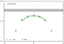
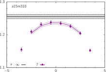
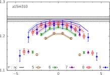
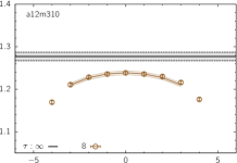
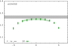
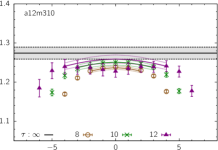
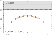
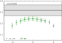
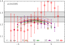
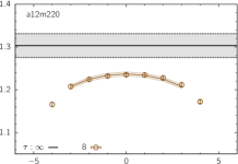
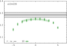
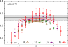
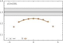
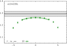
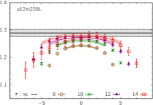
Figure 9: Comparison between the $2^{\ast}$ and $3^{\ast}$ fits to the axial charge $g_{A}^{u-d}$ data from the $a\approx 0.15$ fm (top row) and $a\approx 0.12$ fm (bottom 4 rows) ensembles. The results of the fits are summarized in Table 13 along with the number of points $\mathop{t_{\rm skip}}\nolimits$ skipped. The first two columns show $2^{\ast}$ fits to data versus $t$ at a single value of $\tau$, while the third panel shows the $3^{\ast}$ fit using data at multiple values of $\tau$. The labels give the ensemble ID, and the values of $\tau$ used in the fits. The $\mathop{\tau\to\infty}\nolimits$ value is given by the grey band in each panel.

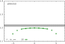
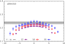
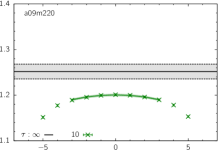
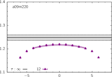
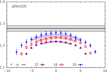
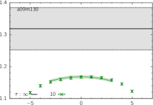
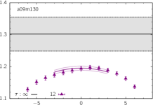
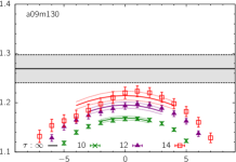
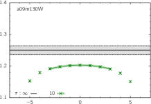
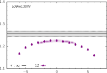
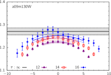
Figure 10: Comparison between the $2^{\ast}$ and $3^{\ast}$ fits to the axial charge $g_{A}^{u-d}$ data from the $a\approx 0.09$ fm ensembles. The rest is the same as in Fig. 9.

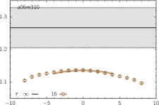
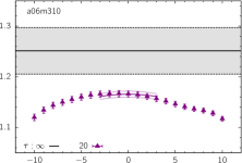
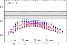
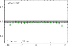
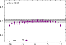
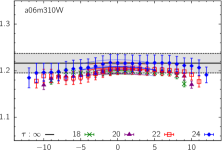
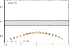
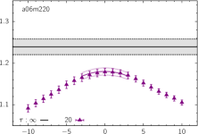
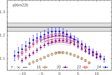
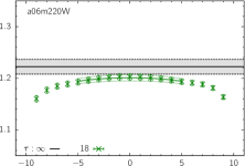
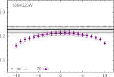
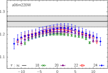
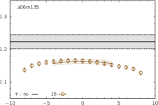
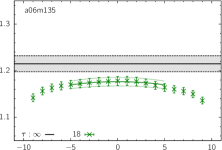
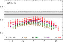
Figure 11: Comparison between the $2^{\ast}$ and $3^{\ast}$ fits to the axial charge $g_{A}^{u-d}$ data from the $a\approx 0.06$ fm ensembles. The rest is the same as in Fig. 9.

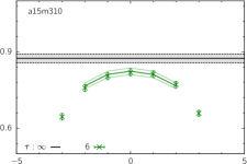
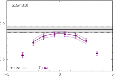
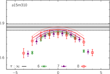
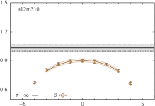
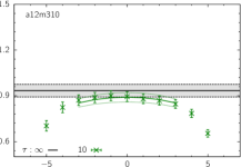
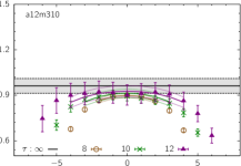
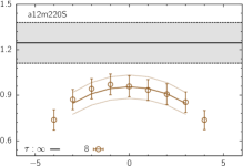
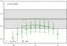
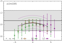
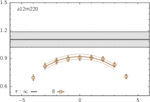
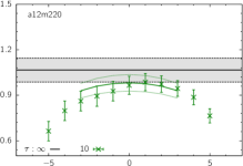
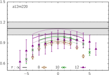
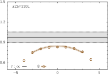
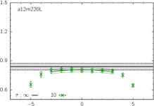
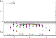
Figure 12: Comparison between the $2^{\ast}$ and $2-$state fits to the scalar charge $g_{S}^{u-d}$ data from the $a\approx 0.15$ fm (top row) and $a\approx 0.12$ fm (bottom 4 rows) ensembles. The rest is the same as in Fig. 9.

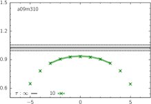
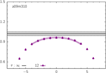
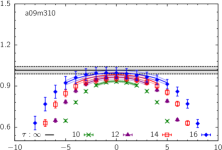
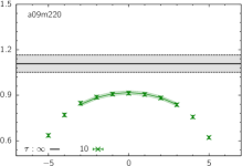
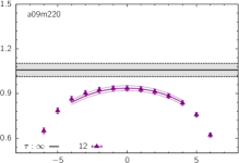
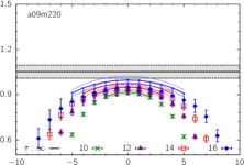
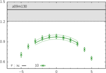
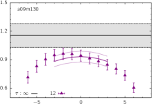
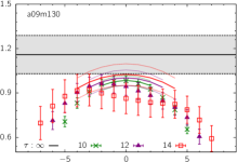
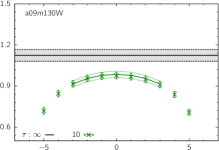
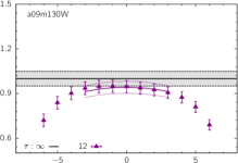
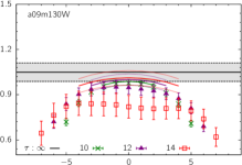
Figure 13: Comparison between the $2^{\ast}$ and $2-$state fits to the scalar charge $g_{S}^{u-d}$ data from the $a\approx 0.09$ fm ensembles. The rest is the same as in Fig. 9.

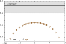
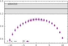
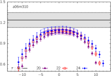
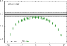
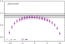
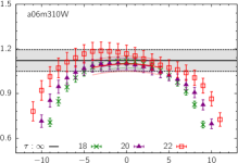
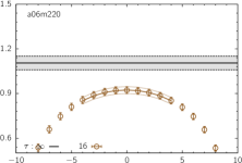
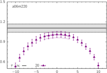
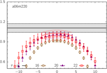
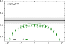
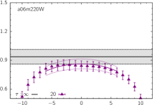
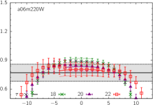
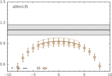
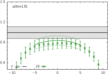
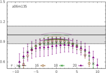
Figure 14: Comparison between the $2^{\ast}$ and $2-$state fits to the scalar charge $g_{S}^{u-d}$ data from the $a\approx 0.06$ fm ensembles. The rest is the same as in Fig. 9.

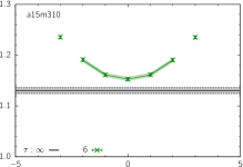
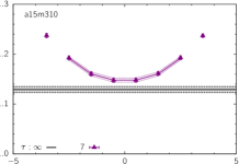
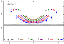
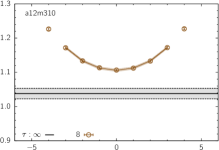
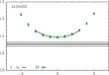
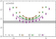
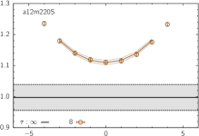
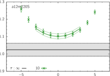
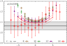
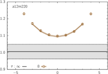
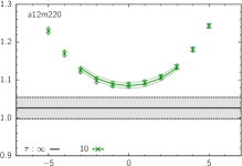
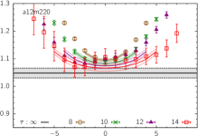
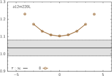
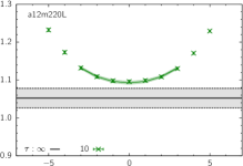
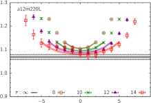
Figure 15: Comparison between the $2^{\ast}$ and $3^{\ast}$ fits to the tensor charge $g_{T}^{u-d}$ data from the $a\approx 0.15$ fm (top row) and $a\approx 0.12$ fm (bottom 4 rows) ensembles. The rest is the same as in Fig. 9.

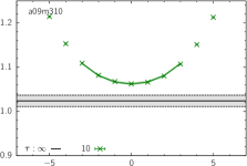
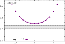
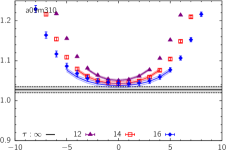
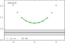
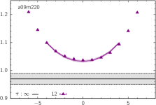
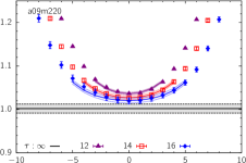
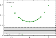
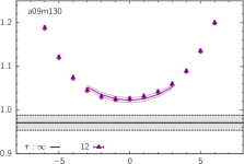
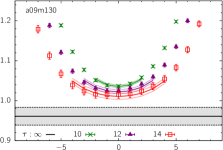
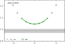
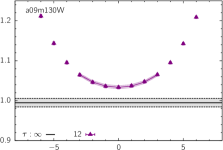
Figure 16: Comparison between the $2^{\ast}$ and $3^{\ast}$ fits to the tensor charge $g_{T}^{u-d}$ data from the $a\approx 0.09$ fm ensembles. The rest is the same as in Fig. 9.

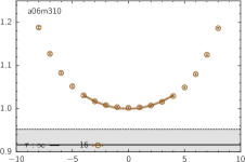
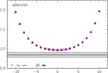
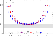
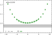
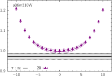
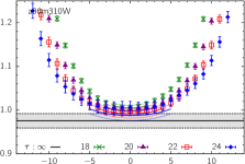
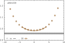
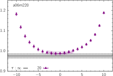
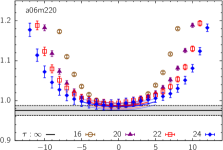
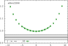
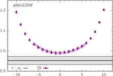
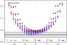
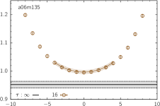
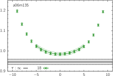
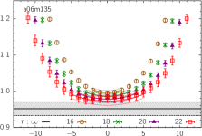
Figure 17: Comparison between the $2^{\ast}$ and $3^{\ast}$ fits to the tensor charge $g_{T}^{u-d}$ data from the $a\approx 0.06$ fm ensembles. The rest is the same as in Fig. 9.

• The new high statistics data for ensembles $a09m310$, $a09m220$ and $a09m130W$ were generated using the smearing parameter $\sigma=7$. This corresponds to a r.m.s. radius of $\approx 7.5$ in lattice units or roughly 0.66 fm. As discussed in Sec. III and shown in Figs. 9–17, increasing $\sigma$ from $5.5$ to $7.0$ reduces the ESC at a given source-sink separation $\tau$.

• The two-point correlation functions are analyzed keeping up to four states in the spectral decomposition. Previous work was based on keeping two states.

• The three-point functions are analyzed keeping up to three states in the spectral decomposition of the spectral functions. Previous work was based on keeping two states.

We find that the new higher precision data significantly improved the ESC fits and the final combined CCFV fit used to obtain results in the limits $a\to 0$, the pion mass $M_{\pi}\to 135$ MeV and the lattice volume $M_{\pi}L\to\infty$.

II.1 Correlation Functions

We use the following interpolating operator $\chi$ to create$/$annihilate the nucleon state:

$$\chi(x)=\epsilon^{abc}\left[{q_{1}^{a}}^{T}(x)C\gamma_{5}\frac{(1\pm\gamma_{4})}{2}q_{2}^{b}(x)\right]q_{1}^{c}(x)\,,$$ (1)

with $\{a,b,c\}$ labeling the color indices, $C=\gamma_{0}\gamma_{2}$ the charge conjugation matrix, and $q_{1}$ and $q_{2}$ denoting the two different flavors of light quarks. The nonrelativistic projection $(1\pm\gamma_{4})/2$ is inserted to improve the signal, with the plus and minus signs applied to the forward and backward propagation in Euclidean time, respectively Gockeler et al. (1996). At zero momentum, this operator couples only to the spin-$\frac{1}{2}$ state.

The zero momentum 2-point and 3-point nucleon correlation functions are defined as

$${\mathbf{C}}_{\alpha\beta}^{\text{2pt}}(\tau) =\sum_{\mathbf{x}}\langle 0|\chi_{\alpha}(\tau,\mathbf{x})\overline{\chi}_{\beta}(0,\mathbf{0})|0\rangle\,,$$ (2)

$${\mathbf{C}}_{\Gamma;\alpha\beta}^{\text{3pt}}(t,\tau) =\sum_{\mathbf{x},\mathbf{x^{\prime}}}\langle 0|\chi_{\alpha}(\tau,\mathbf{x})\mathcal{O}_{\Gamma}(t,\mathbf{x^{\prime}})\overline{\chi}_{\beta}(0,\mathbf{0})|0\rangle\,,$$ (3)

where $\alpha$ and $\beta$ are spinor indices. The source is placed at time slice $0$, $\tau$ is the sink time slice, and $t$ is an intermediate time slice at which the local quark bilinear operator $\mathcal{O}_{\Gamma}^{q}(x)=\bar{q}(x)\Gamma q(x)$ is inserted. The Dirac matrix $\Gamma$ is $1$, $\gamma_{4}$, $\gamma_{i}\gamma_{5}$ and $\gamma_{i}\gamma_{j}$ for scalar (S), vector (V), axial (A) and tensor (T) operators, respectively. In this work, subscripts $i$ and $j$ on gamma matrices run over $\{1,2,3\}$, with $i<j$.

The nucleon charges $g_{\Gamma}^{q}$ are obtained from the ground state matrix element $\langle N(p,s)|\mathcal{O}_{\Gamma}^{q}|N(p,s)\rangle$, that, in turn, are extracted using the spectral decomposition of the 2- and 3-point correlation functions. They are related as

$$\langle N(p,s)|\mathcal{O}_{\Gamma}^{q}|N(p,s)\rangle=g_{\Gamma}^{q}\bar{u}_{s}(p)\Gamma u_{s}(p)$$ (4)

with spinors satisfying

$$\sum_{s}u_{s}(p)\bar{u}_{s}(p)=\frac{E_{\mathbf{p}}\gamma_{4}-i\vec{\gamma}\cdot\vec{p}+M_{N}}{2E_{\mathbf{p}}}\,.$$ (5)

To extract the charges, we construct the projected 2- and 3-point correlation functions

$$C^{\text{2pt}}(t) ={\langle\operatorname{Tr}[\mathcal{P}_{\text{2pt}}{\mathbf{C}}^{\text{2pt}}(t)]\rangle}$$ (6)

$$C_{\Gamma}^{\text{3pt}}(t,\tau) =\langle\operatorname{Tr}[\mathcal{P}_{\rm 3pt}{\mathbf{C}}_{\Gamma}^{\text{3pt}}(t,\tau)]\rangle\,.$$ (7)

The operator $\mathcal{P}_{\text{2pt}}=(1\pm\gamma_{4})/2$ is used to project on to the positive parity contribution for the nucleon propagating in the forward (backward) direction. For the connected 3-point contributions, $\mathcal{P}_{\rm 3pt}=\mathcal{P}_{\text{2pt}}(1+i\gamma_{5}\gamma_{3})$ is used. Note that the $C_{\Gamma}^{\text{3pt}}(t,\tau)$ defined in Eq. (7) becomes zero if $\Gamma$ anticommutes with $\gamma_{4}$, so only $\Gamma=1$, $\gamma_{4}$, $\gamma_{i}\gamma_{5}$ and $\gamma_{i}\gamma_{j}$ elements of the Clifford algebra survive. The fits used to extract the masses, amplitudes and matrix elements from the 2- and 3-point functions, defined in Eqs. (6) and (7), are discussed in Sec. III.

II.2 High Statistics Using the Truncated Solver Method

We have carried out high-statistics calculation on all the ensembles using the truncated solver method with bias correction Bali et al. (2010); Blum et al. (2013). In this method, correlation functions are constructed using quark propagators inverted with high precision (HP) and low precision (LP) using the multigrid algorithm. The bias corrected correlators on each configuration are then given by

$$C^{\text{imp}} =\frac{1}{N_{\text{LP}}}\sum_{i=1}^{N_{\text{LP}}}C_{\text{LP}}(\mathbf{x}_{i}^{\text{LP}})$$

$$+ \frac{1}{N_{\text{HP}}}\sum_{i=1}^{N_{\text{HP}}}\left[C_{\text{HP}}(\mathbf{x}_{i}^{\text{HP}})-C_{\text{LP}}(\mathbf{x}_{i}^{\text{HP}})\right]\,,$$ (8)

where $C_{\text{LP}}$ and $C_{\text{HP}}$ are the 2- and 3-point correlation functions constructed using LP and HP quark propagators, respectively, and $\mathbf{x}_{i}^{\text{LP}}$ and $\mathbf{x}_{i}^{\text{HP}}$ are the source positions for the two kinds of propagator inversion. The LP stopping criteria, defined as $r_{\rm LP}\equiv|{\rm residue}|_{\rm LP}/|{\rm source}|$ varied between $10^{-3}$ and $5\times 10^{-4}$, while that for the HP calculations between $10^{-7}$ and $10^{-8}$.

As discussed in Ref. Yoon et al. (2016), to reduce statistical correlations between measurements, $N_{\text{HP}}$ maximally separated time slices were selected randomly on each configuration and on each of these time slices, $N_{\text{LP}}/N_{\text{HP}}$ LP source positions were again selected randomly. The number of sources, $N_{\text{LP}}$ and $N_{\text{HP}}$, used are given in Table 1. An important conclusion based on all our calculations with $O(10^{5})$ measurements of nucleon charges and form factors carried out so far (see Refs. Bhattacharya et al. (2015a, 2016); Yoon et al. (2016, 2017); Gupta et al. (2017)), is that the difference between the LP and the bias corrected estimates (or the HP) is smaller than the statistical errors.

To further reduce the computational cost, we also used the coherent sequential source method discussed in Ref. Yoon et al. (2016). Typically, we constructed four HP or LP sequential sources on four sink time slices, and added them to obtain the coherent source. A single inversion was then performed to construct the coherent sequential propagator. This was then contracted with the four original propagators to construct four measurements of each three-point function. All of these propagators were held in the computer memory to remove the I/O overhead.

Our final errors are obtained using a single elimination jackknife analysis over the configurations, that is, we first construct the average defined in Eq. (8) on each configuration. Because of this “binning” of the data, we do not need to correct the jackknife estimate of the error for correlations between the $N_{\text{LP}}$ LP measurements per configuration.

III Excited-State Contamination

To extract the nucleon charges we need to evaluate the matrix elements of the currents between ground-state nucleons. The lattice nucleon interpolating operator given in Eq. (1), however, couples to the nucleon, all its excitations and multiparticle states with the same quantum numbers. Previous lattice calculations have shown that the ESC can be large. In our earlier works Bhattacharya et al. (2015a, 2016); Yoon et al. (2017, 2016), we have shown that this can be controlled to within a few percent using the strategy summarized below.

The overlap between the nucleon operator and the excited states in the construction of the two- and three-point functions is reduced by using tuned smeared sources when calculating the quark propagators on the HYP smeared HISQ lattices. We construct gauge-invariant Gaussian smeared sources by applying the three-dimensional Laplacian operator, $\nabla^{2}$, $N_{\rm GS}$ number of times, i.e., $(1+\sigma^{2}\nabla^{2}/(4N_{\rm GS}))^{N_{\rm GS}}$ on a delta function source. The input smearing parameters $\{\sigma,N_{\rm GS}\}$ for each ensemble are given in Table 2 along with the resulting root-mean-square radius defined as $\sqrt{\int r^{2}\sqrt{S^{\dagger}S}dr/\int\sqrt{S^{\dagger}S}dr}$. We find that, as a function of distance $r$, the modulus of the sum of the values of the twelve spin-color components at each site, $\sqrt{S^{\dagger}S}$, is well described by a Gaussian, and we use this ansatz to fit the data. The results for the root-mean-square radius given in Table 2 show weak dependence on the lattice spacing or the pion mass for fixed $\sigma$, and are roughly equal to the input $\sigma$. Throughout this work, the same smearing is used at the source and sink points.

The analysis of the two-point functions, $C^{\text{2pt}}$, was carried out keeping four states in the spectral decomposition:

$$C^{\text{2pt}} (t,\bm{p})=$$

$${|{\cal A}_{0}|}^{2}e^{-M_{0}t}+{|{\cal A}_{1}|}^{2}e^{-M_{1}t}\,+$$

$${|{\cal A}_{2}|}^{2}e^{-M_{2}t}+{|{\cal A}_{3}|}^{2}e^{-M_{3}t}\,,$$ (9)

where the amplitudes and the masses of the four states are denoted by ${\cal A}_{i}$ and $M_{i}$, respectively.

In fits including more than two states, the estimates of $M_{i}$ and the ${\cal A}_{i}$ for $i\geq 2$ were sensitive to the choice of the starting time slice $t_{\rm min}$, and the fits were not always stable. The fits were stabilized using the empirical Bayesian procedure described in Ref. Yoon et al. (2017). Examples of the quality of the fits are shown in Figs. 22–29 in Ref. Gupta et al. (2017). The new results for masses and amplitudes obtained from 2-, 3- and 4-state fits are given in Table LABEL:tab:2ptmulti.

In Fig. 1, we compare the efficacy of different smearing sizes in controlling excited states in the 2-point data on the three ensembles $a09m130$, $a06m310$ and $a06m220$. In each case, the onset of the plateau with the larger smearing size occurs at earlier Euclidean time $t$, however, the statistical errors at larger $t$ are larger. The more critical observation is that, while $M_{0}$ overlap, the mass gaps $a\Delta M_{i}$ are significantly different in two cases. Thus the excited state parameters are not well determined even with our high statistics, $O(10^{5})$ measurements, data. More importantly, except for the $a06m310$ case, the mass gap $a\Delta M_{1}$ obtained is much larger than $2aM_{\pi}$, the value expected if $N\pi\pi$ is the lowest excitation. Based on these observations, we conclude that to resolve the excited state spectrum will require a coupled channel analysis with much higher statistics data.

The results of different fits for the bare charges extracted from the three-point data, given in Table 13, indicate that these differences in the mass gaps do not significantly effect the extraction of the charges. At current level of precision, the variations in the values of the mass gaps and the corresponding values for the amplitudes compensate each other in fits to the 2- and 3-point data.

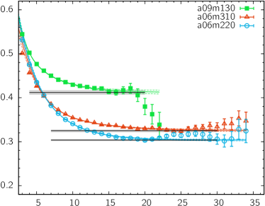
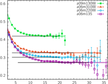
Figure 1: Illustration of the data for the nucleon $M_{\rm eff}$ versus Euclidean time $t$ and the results of the 4-state fit to the 2-point correlation function. We compare the data obtained with two different smearing sizes on three ensembles. In the right panel we also show results for the $a06m135$ ensemble. The onset of the plateau in $M_{\rm eff}$ occurs at earlier $t$ with the larger smearing size but the errors at larger $t$ are also larger.

The analysis of the zero-momentum three-point functions, $C_{\Gamma}^{(3\text{pt})}(t;\tau)$ was carried out retaining three-states in its spectral decomposition:

$$C^{\text{3pt}}_{\Gamma}(t_{f},t,t_{i})=$$

$$|{\cal A}_{0}|^{2}\langle 0|\mathcal{O}_{\Gamma}|0\rangle e^{-aM_{0}(t_{f}-t_{i})}+{}$$

$$|{\cal A}_{1}|^{2}\langle 1|\mathcal{O}_{\Gamma}|1\rangle e^{-aM_{1}(t_{f}-t_{i})}+{}$$

$$|{\cal A}_{2}|^{2}\langle 2|\mathcal{O}_{\Gamma}|2\rangle e^{-aM_{2}(t_{f}-t_{i})}+{}$$

$${\cal A}_{1}{\cal A}_{0}^{*}\langle 1|\mathcal{O}_{\Gamma}|0\rangle e^{-aM_{1}(t_{f}-t)}e^{-aM_{0}(t-t_{i})}+{}$$

$${\cal A}_{0}{\cal A}_{1}^{*}\langle 0|\mathcal{O}_{\Gamma}|1\rangle e^{-aM_{0}(t_{f}-t)}e^{-aM_{1}(t-t_{i})}+{}$$

$${\cal A}_{2}{\cal A}_{0}^{*}\langle 2|\mathcal{O}_{\Gamma}|0\rangle e^{-aM_{2}(t_{f}-t)}e^{-aM_{0}(t-t_{i})}+{}$$

$${\cal A}_{0}{\cal A}_{2}^{*}\langle 0|\mathcal{O}_{\Gamma}|2\rangle e^{-aM_{0}(t_{f}-t)}e^{-aM_{2}(t-t_{i})}+{}$$

$${\cal A}_{1}{\cal A}_{2}^{*}\langle 1|\mathcal{O}_{\Gamma}|2\rangle e^{-aM_{1}(t_{f}-t)}e^{-aM_{2}(t-t_{i})}+{}$$

$${\cal A}_{2}{\cal A}_{1}^{*}\langle 2|\mathcal{O}_{\Gamma}|1\rangle e^{-aM_{2}(t_{f}-t)}e^{-aM_{1}(t-t_{i})}+\ldots\,,$$ (10)

where the source point is at $t_{i}$, the operator is inserted at time $t$, and the nucleon state is annihilated at the sink time slice $t_{f}$. The source-sink separation is $\tau\equiv t_{f}-t_{i}$. The state $|0\rangle$ represents the ground state and $|n\rangle$, with $n>0$, the higher states. The ${\cal A}_{i}$ are the amplitudes for the creation of state $i$ with zero momentum by the nucleon interpolating operator $\chi$. To extract the matrix elements, the amplitudes ${\cal A}_{i}$ and the masses $M_{i}$ are obtained from the 4-state fits to the two-point functions. Note that the insertion of the nucleon at the sink time slice $t_{f}$ and the insertion of the current at time $t$ are both at zero momentum. Thus, by momentum conservation, only the zero momentum projections of the states created at the source time slice contribute to the three-point function.

We calculate the three-point correlation functions for a number of values of the source-sink separation $\tau$ that are listed in Table 1. To extract the desired matrix element $\langle 0|\mathcal{O}_{\Gamma}|0\rangle$, we fit the data at all $\tau$ and $t$ simultaneously using the ansatz given in Eq. (10). In this work, we examine three kinds of fits, $2^{\ast}$-, 2- and $3^{\ast}$-state fits. The $2^{\ast}$-state fit corresponds to keeping terms of the type $\langle 0\lvert\mathcal{O}_{\Gamma}\rvert 0\rangle$ and $\langle 0\lvert\mathcal{O}_{\Gamma}\rvert 1\rangle$. The 2-state fits also include $\langle 1\lvert\mathcal{O}_{\Gamma}\rvert 1\rangle$, and the $3^{\ast}$-state fits further add the $\langle 0\lvert\mathcal{O}_{\Gamma}\rvert 2\rangle$ and $\langle 1\lvert\mathcal{O}_{\Gamma}\rvert 2\rangle$ type terms.

In the simultaneous fit to the data versus $t$ and multiple $\tau$ to obtain $\langle 0\lvert\mathcal{O}_{\Gamma}\rvert 0\rangle$, we skip $\mathop{t_{\rm skip}}\nolimits$ points adjacent to the source and the sink to remove points with the largest ESC. The same $\mathop{t_{\rm skip}}\nolimits$ is used for each $\tau$. The $\mathop{t_{\rm skip}}\nolimits$ selected is a compromise between wanting to include as many points as possible to extract the various terms given in Eq. (10) with confidence, and the errors in and stability of the full covariance matrix used in the fit. In particular, the choice of $\mathop{t_{\rm skip}}\nolimits$ on the $a=0.06$ fm ensembles is the smallest value for which the covariance matrix was invertable and reasonable. These values of $\mathop{t_{\rm skip}}\nolimits$, tuned for each ensemble, are given in Table 13.

To visualize the ESC, we plot the data for the following ratio of correlation functions

$$R_{\Gamma}(t,\tau)=\frac{C_{\Gamma}^{\text{3pt}}(t,\tau)}{C^{\text{2pt}}(\tau)}\to g_{\Gamma}\,,$$ (11)

in Figs. 9–17 and show the various fits corresponding to the results in Table 13. In the limit $t\to\infty$ and $\tau-t\to\infty$, this ratio converges to the charge $g_{\Gamma}$. At short times, the ESC is manifest in all cases. For sufficiently large $\tau$, the data should exhibit a flat region about $\tau/2$, and the value should become independent of $\tau$. The current data for $g_{A}$, $g_{S}$ and $g_{T}$, with $\tau$ up to about 1.4 fm, do not provide convincing evidence of this desired asymptotic behavior. To obtain $\langle 0\lvert\mathcal{O}_{\Gamma}\rvert 0\rangle$, we use the three-state ansatz given in Eq. (10).

On the three ensembles, $a09m130$, $a06m310$ and $a06m220$, we can compare the data with two different smearing sizes given in Table 1. We find a significant reduction in the ESC in the axial and scalar charges on increasing the smearing size. Nevertheless, the 2- and $3^{\ast}$-state fits and the two calculations give consistent estimates for the ground state matrix elements. The agreement between these four estimates has increased our confidence in the control over ESC. The results for $g_{S}^{u-d}$, obtained using $2$-state fits, have larger uncertainty as discussed in Sec. III.1, but are again consistent except those from the $a06m220$ ensemble.

This higher statistics study of the ESC confirms many features discussed in Ref. Bhattacharya et al. (2016):

• The ESC is large in both $g_{A}^{u-d}$ and $g_{S}^{u-d}$, and the convergence to the $\mathop{\tau\to\infty}\nolimits$ value is monotonic and from below.

• The ESC is $g_{T}^{u-d}$ is $\lesssim 10\%$ for $\tau>1$ fm, and the convergence to the $\mathop{\tau\to\infty}\nolimits$ value is also monotonic but from above.

• The ESC in $g_{A}^{u-d}$ and $g_{S}^{u-d}$ is reduced on increasing the size of the smearing, but $g_{T}^{u-d}$ is fairly insensitive to the smearing size.

• For a given number of measurements at the same $\tau$ and $t$, the statistical precision of $g_{T}^{u-d}$ is slightly better than that of $g_{A}^{u-d}$. The data for $g_{S}^{u-d}$ is noisy, especially at the larger values of $\tau$. On many ensembles, it does not exhibit a monotonic increase with $\tau$. To get $g_{S}^{u-d}$ with the same precision as in $g_{A}^{u-d}$ currently will require $\approx 5$ times the statistics.

• The data for each charge and for each source-sink separation $\tau$ becomes symmetric about $\tau/2$ with increasing statistical precision. This is consistent with the $\cosh(t-\tau/2)$ behavior predicted by Eq. (10) for each transition matrix element.

• The variations in the results with the fit ranges selected for fits to the two-point functions and the number, $\mathop{t_{\rm skip}}\nolimits$, of points skipped in the fits to the three-point data decrease with the increased statistical precision.

• Estimates from the $2$- and the $3^{\ast}$-state fits overlap for all fourteen measurements of $g_{A}^{u-d}$ and $g_{T}^{u-d}$.

• The $3^{\ast}$-state fits for $g_{S}^{u-d}$ are not stable in all cases and many of the parameters are poorly determined. To extract our best estimates, we use 2-state fits.

• The largest excited-state contribution comes from the $\langle 0|O_{\Gamma}|1\rangle$ transition matrix elements. We, therefore discuss a poor person’s recipe to get estimates based on the $2^{\ast}$ fits in Sec. III.1 that are useful when data at only one value of $\tau$ are available.

Our conclusion on ESC is that with $O(10^{5})$ measurements, $3^{\ast}$ fits, the choice of smearing parameters used and the values of $\tau$ simulated, the excited-state contamination in $g_{A}^{u-d}$ and $g_{T}^{u-d}$ has been controlled to within a couple of percent, i.e., the size of the quoted errors. The errors in $g_{S}^{u-d}$ are at the 5%–10% level, and we take results from the 2-state fit as our best estimates. In general, for calculations by other groups when data with reasonable precision are available only at a single value of $\tau$, we show that the $2^{\ast}$ fit gives a much better estimate than the plateau value.

III.1 A poor person’s recipe and $g_{S}^{u-d}$

Our high statistics calculations allow us to develop the following poor person’s recipe for estimating the ground state matrix element when data are available only at a single value of $\tau$. To illustrate this, we picked two values with $\tau\approx 1$ fm ($\tau=\{6,7\},\{8,10\},\{10,12\},\{16,18,20\}$ in lattice units for the $a\approx 0.15,0.12,0.09,0.06$ ensembles) for which we have reasonably precise data at all values of $t$ and for all three isovector charges. We then compared the estimates of the charges from the $2^{\ast}$ fit to data at these values of $\tau$ with our best estimate from the $3^{\ast}$ fit (2-state for $g_{S}^{u-d}$) to the data at multiple $\tau$ and $t$. Fits for all ensembles are shown in Figs. 9–17 and the results collected in Table 13.

In the case of $g_{A}^{u-d}$ and $g_{T}^{u-d}$ we get overlapping results results converging to the $3^{\ast}$ value. This suggests that, within our statistical precision, all the excited-state terms that behave as $\cosh\Delta M(t-\tau/2)$ in the spectral decomposition are well-approximated by the single term proportional to $\langle 0|{\cal{O}}|1\rangle$ in the $2^{\ast}$ fit. Isolating this ESC is, therefore, essential. Also, the remainder, the sum of all the terms independent of $t$ is small. This explains why the values of the excited state matrix elements $\langle 1|{\cal{O}}|1\rangle$ and $\langle 0|{\cal{O}}|2\rangle$, given in Table 4, are poorly determined.

We further observe that in our implementation of the lattice calculations—HYP smoothing of the lattices plus the Gaussian smearing of the quark sources—the product $(M_{1}-M_{0})\times\tau$ is $\gtrsim 1$ for $\tau\approx 1$ fm, i.e., $(M_{1}-M_{0})\gtrsim 200$ MeV. Since this condition holds for the physical nucleon spectrum, it is therefore reasonable to expect that the charges extracted from a $2^{\ast}$ fit to data with $\tau\gtrsim 1$ fm are a good approximation to the $\mathop{\tau\to\infty}\nolimits$ value, whereas the value at the midpoint $t=\tau/2$ (called the plateau value) is not. This is supported by the data for $g_{A}^{u-d}$ and $g_{T}^{u-d}$ shown in Table 13; there is much better consistency between the $3^{\ast}$ results and $2^{\ast}$ fits to data with a single values of $\tau\gtrsim 1$ fm versus the plateau value.

In this work, the reason for considering such a recipe is that estimates of $g_{S}^{u-d}$ have much larger statistical errors, because of which the data at the larger values of $\tau$ do not, in all cases, exhibit the expected monotonic convergence in $\tau$ and have large errors. As a result, on increasing $n$ in an $n$-state fit to data with multiple values of $\tau$ does not always give a better or converged value. We, therefore, argue that to obtain the best estimates of $g_{S}^{u-d}$ one can make judicious use of this recipe, i.e., use $2^{\ast}$ fits to the data with the largest value of $\tau$ that conforms with the expectation of monotonic convergence from below. In our case, based on such analyses we conclude that the 2-state fits are more reliable than $3^{\ast}$ fits for $g_{S}^{u-d}$. These fourteen values of $g_{S}^{u-d}$ used in the final analysis are marked with the superscript ^† in Table 13. The same strategy is followed for obtaining the connected contribution to the isoscalar charges, $g_{S}^{u+d}$, that are given in Table 14.

ID	$g_{A}^{u}$	$g_{A}^{d}$	$g_{A}^{u-d}$	$g_{S}^{u}$	$g_{S}^{d}$	$g_{S}^{u-d}$	$g_{T}^{u}$	$g_{T}^{d}$	$g_{T}^{u-d}$
$a15m310$	0.937(06)	$-$0.313(04)	1.250(07)	3.10(08)	2.23(06)	0.87(03)	0.901(06)	$-$0.219(04)	1.121(06)
$a12m310$	0.946(15)	$-$0.328(09)	1.274(15)	3.65(13)	2.69(09)	0.96(05)	0.859(12)	$-$0.206(07)	1.065(13)
$a12m220S$	0.934(43)	$-$0.332(27)	1.266(44)	5.23(49)	4.23(40)	1.00(26)	0.816(44)	$-$0.249(33)	1.065(39)
$a12m220$	0.947(22)	$-$0.318(13)	1.265(21)	4.83(35)	3.72(29)	1.11( 9)	0.847(17)	$-$0.201(11)	1.048(18)
$a12m220L$	0.942(09)	$-$0.347(08)	1.289(13)	4.21(29)	3.34(26)	0.87(04)	0.846(11)	$-$0.203(05)	1.069(11)
$a09m310$	0.930(07)	$-$0.308(04)	1.238(08)	3.60(12)	2.58(10)	1.02(03)	0.824(07)	$-$0.203(03)	1.027(07)
$a09m220$	0.945(12)	$-$0.334(06)	1.279(13)	4.46(19)	3.41(16)	1.05(04)	0.799(10)	$-$0.203(05)	1.002(10)
$a09m130$	0.919(20)	$-$0.350(16)	1.269(28)	5.87(49)	4.71(41)	1.16(13)	0.765(20)	$-$0.196(10)	0.961(22)
$a09m130W$	0.935(14)	$-$0.336(08)	1.271(15)	5.28(17)	4.23(14)	1.05(06)	0.797(12)	$-$0.203(06)	1.000(12)
$a06m310$	0.923(25)	$-$0.320(15)	1.243(27)	4.48(33)	3.24(24)	1.24(11)	0.785(20)	$-$0.197(11)	0.982(20)
$a06m310W$	0.906(22)	$-$0.310(16)	1.216(21)	4.06(16)	2.94(11)	1.12(07)	0.784(15)	$-$0.192(08)	0.975(16)
$a06m220$	0.912(13)	$-$0.323(13)	1.235(18)	4.40(13)	3.29(09)	1.11(07)	0.779(10)	$-$0.197(10)	0.975(12)
$a06m220W$	0.917(24)	$-$0.341(15)	1.257(24)	4.32(21)	3.55(18)	0.77(09)	0.764(21)	$-$0.198(11)	0.962(22)
$a06m135$	0.917(22)	$-$0.323(13)	1.240(26)	5.26(22)	4.26(15)	1.00(13)	0.768(17)	$-$0.183(10)	0.952(19)

Table 3: Results for the bare connected contributions to the various charges.

III.2 Transition and excited state matrix elements

The only transition matrix element that has been estimated with some degree of confidence is $\langle 0|\mathcal{O}_{\Gamma}|1\rangle$ as can be inferred from the results given in Table 4. Also including information from Figs. 9–17, our qualitative conclusions on it are as follows:

• Estimates of $\langle 0|\mathcal{O}_{A}|1\rangle$ vary between $-0.1$ and $-0.3$ and account for the negative curvature evident in the figures. All ground-state estimates of $g_{A}^{u-d}$ converge from below.

• Estimates of $\langle 0|\mathcal{O}_{S}|1\rangle$ vary between $-0.2$ and $-0.5$ and account for the larger negative curvature observed in the figures. All ground-state estimates of $g_{S}^{u-d}$ also converge from below.

• Estimates of $\langle 0|\mathcal{O}_{T}|1\rangle$ vary between 0.1 and 0.3 and account for the positive curvature evident in the figures. The ground-state estimates of $g_{T}^{u-d}$ converge from above in all cases.

Our long term goal is to improve the precision of these calculations to understand and extract an infinite volume continuum limit value for the transition matrix elements.

III.3 A caveat in the analysis of the isoscalar charges $g_{A,S,T}^{u+d}$ keeping only the connected contribution

In this paper, we have analyzed only the connected contributions to the isoscalar charges $g_{A,S,T}^{u+d}$. The disconnected contributions are not included as they are not available for all the ensembles, and are analyzed for different, typically smaller, values of source-sink separation $\tau$ because of the lower quality of the statistical signal. Since the proper way to extract the isoscalar charges is to first add the connected and disconnected contributions and then perform the fits using the lattice QCD spectral decomposition to remove excited state contamination, analyzing only the connected contribution introduces an approximation. Isoscalar charges without a disconnected contribution can be defined in a partially quenched theory with an additional quark with flavor $u^{\prime}$. However, in this theory the Pauli exclusion principle does not apply between the $u$ and $u^{\prime}$ quarks. The upshot of this is that the spectrum of states in the partially quenched theory is larger, for example, an intermediate $u^{\prime}ud$ state would be the analogue of a $\Lambda$ baryon. Thus, the spectral decomposition for this partially quenched theory and QCD is different. The problem arises because our n-state fits assume the QCD spectrum since we take the amplitudes and masses of states from the QCD 2-point function when fitting the 3-point function using Eq. (10). One could make fits to 3-point functions leaving all the parameters in Eq. (10) free, but then even 2-state fits become poorly constrained with current data.

We assume that, in practice, the effect due to using the QCD rather than the partially quenched QCD spectra to fit the connected contribution versus $t$ and $\tau$ to remove ESC is smaller than the quoted errors. First, the difference between the plateau value in our largest $\tau$ data and the $\tau\to\infty$ value is a few percent effect, so that any additional systematic is well within the quoted uncertainty. Furthermore, for the tensor charges the disconnected contribution is tiny and consistent with zero, so for the tensor charges one can ignore this caveat. For the axial and scalar charges, the disconnected contribution is between 10%–20% of the connected, so we are neglecting possible systematic effects due to extrapolating the connected and disconnected contributions separately.

	Axial			Scalar		Tensor
ID	$\langle 0|\mathcal{O}_{A}|1\rangle$	$\langle 1|\mathcal{O}_{A}|1\rangle$	$\langle 0|\mathcal{O}_{A}|2\rangle$	$\langle 0|\mathcal{O}_{S}|1\rangle$	$\langle 1|\mathcal{O}_{S}|1\rangle$	$\langle 0|\mathcal{O}_{T}|1\rangle$	$\langle 1|\mathcal{O}_{T}|1\rangle$	$\langle 0|\mathcal{O}_{T}|2\rangle$
$a15m310$	$-$0.044( 37)	$-$2.06(1.3)	$-$0.08( 5)	$-$0.37( 3)	3.6(4.6)	0.31( 4)	$-$2.72(1.2)	$-$0.18( 7)
$a12m310$	$-$0.208( 94)	1.40(2.4)	0.07( 4)	$-$0.72( 9)	8.5(10.)	0.32( 8)	$-$0.82(2.2)	0.08( 4)
$a12m220S$	$-$0.119( 77)	1.46(60)	0.03(10)	$-$0.42(13)	3.8(5.7)	0.19( 8)	0.13(62)	0.10(11)
$a12m220$	$-$0.047( 52)	0.33(76)	$-$0.08( 5)	$-$0.38(11)	$-$ 2.8(3.6)	0.21( 5)	0.07(59)	0.12( 4)
$a12m220L$	$-$0.084( 25)	$-$0.21(73)	$-$0.05( 3)	$-$0.38(12)	4.6(2.7)	0.19( 2)	$-$0.04(43)	0.09( 4)
$a09m310$	$-$0.095( 20)	$-$1.45(1.9)	0.11( 6)	$-$0.39( 4)	0.7(1.5)	0.20( 2)	0.17(1.1)	0.04( 6)
$a09m220$	$-$0.153( 34)	$-$0.44(98)	0.07( 4)	$-$0.47( 5)	1.4(1.0)	0.16( 3)	0.44(60)	0.13( 3)
$a09m130$	$-$0.092( 26)	0.65(19)	0.03( 4)	$-$0.42( 7)	2.0(1.2)	0.17( 3)	0.78(14)	0.08( 4)
$a09m130W$	$-$0.098( 26)	$-$0.46(94)	0.06( 6)	$-$0.28( 4)	2.2(2.2)	0.18( 3)	0.37(71)	0.11( 6)
$a06m310$	$-$0.075( 41)	0.18(51)	$-$0.00( 1)	$-$0.41( 6)	1.2(1.4)	0.14( 5)	$-$0.20(60)	$-$0.08( 9)
$a06m310W$	$-$0.093(124)	$-$0.56(4.5)	$-$0.02(35)	$-$0.44( 9)	10.6(15.)	0.22(12)	0.41(3.9)	0.04(36)
$a06m220$	$-$0.184( 40)	0.43(38)	0.28(13)	$-$0.32( 4)	$-$ 0.3(1.1)	0.09( 4)	0.33(32)	0.05(12)
$a06m220W$	$-$0.249(127)	1.2(2.2)	0.32(25)	$-$0.33(14)	23.4(20.)	0.29(13)	$-$1.86(3.0)	$-$0.17(25)
$a06m135$	$-$0.137( 47)	0.81(41)	0.20(13)	$-$0.32( 6)	2.4(3.1)	0.12( 5)	0.82(39)	0.07(12)

Table 4: Estimates of the leading ratios $\langle 0|\mathcal{O}_{\Gamma}|1\rangle/\langle 0|\mathcal{O}_{\Gamma}|0\rangle$, $\langle 1|\mathcal{O}_{\Gamma}|1\rangle/\langle 0|\mathcal{O}_{\Gamma}|0\rangle$, and $\langle 0|\mathcal{O}_{\Gamma}|2\rangle/\langle 0|\mathcal{O}_{\Gamma}|0\rangle$ for the transition and excited state matrix elements in the case of the isovector charges. For the scalar charge, $\langle 0|\mathcal{O}_{\Gamma}|2\rangle/\langle 0|\mathcal{O}_{\Gamma}|0\rangle$ is not given since our final results are from the $2$-state fit that are marked with ^† in Table 13.

IV Renormalization of Operators

The renormalization constants $Z_{A}$, $Z_{V}$, $Z_{S}$ and $Z_{T}$ of the isovector quark bilinear operators are calculated in the regularization-independent symmetric momentum-subtraction (RI-sMOM) scheme Martinelli et al. (1995); Sturm et al. (2009). We followed the methodology given in Refs. Bhattacharya et al. (2015a, 2016) and refer the reader to it for details. Results based on the six ensembles, a12m310, a12m220, a09m310, a09m220, a06m310 and a06m220, obtained in Refs. Bhattacharya et al. (2015a, 2016) are summarized in Table 5 along with the new results on the $a15m310$ ensemble. We briefly summarize the method below for completeness.

The calculation was done as follows: starting with the lattice results obtained in the RI-sMOM scheme at a given Euclidean four-momentum squared $Q^{2}$, we first convert them to the $\overline{\text{MS}}$ scheme at the same scale (horizontal matching) using two-loop perturbative relations expressed in terms of the coupling constant $\alpha_{\overline{\text{MS}}}(Q^{2})$ Gracey (2011). This estimate at $\mu^{2}=Q^{2}$, is then run in the continuum in the $\overline{\text{MS}}$ scheme to $2\mathop{\rm GeV}\nolimits$ using the 3-loop anomalous dimension relations for the scalar and tensor bilinears Gracey (2000); Olive et al. (2014). These data are labeled by the $Q^{2}$ in the original RI-sMOM scheme and suffer from artifacts due to nonperturbative effects and the breaking of the Euclidean $O(4)$ rotational symmetry down to the hypercubic group. To get the final estimate, we fit these data versus $Q^{2}$ using an ansatz motivated by the form of possible artifacts as discussed in Refs. Bhattacharya et al. (2015a, 2016).

We find that the final renormalization factors on ensembles with constant $a$ show no significant dependence versus $M_{\pi}$. We, therefore, average the results at different $M_{\pi}$ to get the mass-independent values at each $a$.

In Table 5, we also give the results for the ratios $Z_{A}/Z_{V}$, $Z_{S}/Z_{V}$, and $Z_{T}/Z_{V}$ that show much smaller $O(4)$ breaking, presumably because some of the systematics cancel. From the individual data and the two ratios, $Z_{\Gamma}/Z_{V}$ and $g_{\Gamma}/g_{V}^{u-d}$, we calculate the renormalized charges in two ways: $Z_{\Gamma}\times g_{\Gamma}$ and $(Z_{\Gamma}/Z_{V})\times(g_{\Gamma}/g_{V}^{u-d})$ with $Z_{V}g_{V}^{u-d}=1$ since the conservation of the vector current. These two sets of renormalized charges are given in Table 6.

ID	$Z_{A}^{u-d}$	$Z_{S}^{u-d}$	$Z_{T}^{u-d}$	$Z_{V}^{u-d}$	$Z_{A}^{u-d}/Z_{V}^{u-d}$	$Z_{S}^{u-d}/Z_{V}^{u-d}$	$Z_{T}^{u-d}/Z_{V}^{u-d}$
$a=0.15$ fm	$0.96(2)$	$0.94(4)$	$0.95(3)$	$0.92(2)$	$1.05(2)$	$1.02(5)$	$1.02(3)$
$a=0.12$ fm	$0.95(3)$	$0.90(4)$	$0.94(4)$	$0.91(2)$	$1.045(09)$	$0.986(09)$	$1.034(34)$
$a=0.09$ fm	$0.95(4)$	$0.88(2)$	$0.98(4)$	$0.92(2)$	$1.034(11)$	$0.955(49)$	$1.063(29)$
$a=0.06$ fm	$0.97(3)$	$0.86(3)$	$1.04(3)$	$0.95(1)$	$1.025(09)$	$0.908(40)$	$1.100(25)$

Table 5: The final mass-independent isovector renormalization constants $Z_{A}^{u-d}$, $Z_{S}^{u-d}$, $Z_{T}^{u-d}$, $Z_{V}^{u-d}$ and the ratios $Z_{A}^{u-d}/Z_{V}^{u-d}$, $Z_{S}^{u-d}/Z_{V}^{u-d}$ and $Z_{T}^{u-d}/Z_{V}^{u-d}$ in the $\overline{\text{MS}}$ scheme at 2 GeV at the four values of the lattice spacing used in our analysis. Results for the $a=0.12$, $a=0.09$ and $a=0.06$ fm ensembles are reproduced from Ref. Bhattacharya et al. (2016).

	$g_{\Gamma}^{u-d,{\rm bare}}/g_{V}^{u-d,{\rm bare}}\times Z_{\Gamma}^{u-d}/Z_{V}^{u-d}$			$g_{\Gamma}^{u-d,{\rm bare}}\times Z_{\Gamma}^{u-d}$
ID	$g_{A}^{u-d}$	$g_{S}^{u-d}$	$g_{T}^{u-d}$	$g_{A}^{u-d}$	$g_{S}^{u-d}$	$g_{T}^{u-d}$	$g_{V}^{u-d,{\rm bare}}$	$Z_{V}g_{V}^{u-d,{\rm bare}}$
$a15m310$	1.228(25)	0.828(049)	1.069(32)	1.200(26)	0.816(044)	1.065(34)	1.069(04)	0.983(22)
$a12m310$	1.251(19)	0.891(045)	1.035(37)	1.210(41)	0.865(058)	1.001(44)	1.064(05)	0.968(22)
$a12m220S$	1.224(44)	0.916(233)	1.019(53)	1.203(56)	0.903(237)	1.001(56)	1.081(18)	0.983(27)
$a12m220$	1.234(25)	1.024(086)	1.011(38)	1.202(43)	1.001(096)	0.985(45)	1.071(09)	0.975(23)
$a12m220L$	1.262(17)	0.807(039)	1.035(36)	1.225(41)	0.786(052)	1.005(44)	1.067(04)	0.971(21)
$a09m310$	1.235(15)	0.936(054)	1.054(30)	1.176(50)	0.893(031)	1.007(42)	1.045(03)	0.962(20)
$a09m220$	1.260(19)	0.958(063)	1.015(30)	1.215(53)	0.926(044)	0.982(41)	1.053(03)	0.969(21)
$a09m130$	1.245(32)	1.050(128)	0.969(35)	1.206(57)	1.019(116)	0.942(44)	1.052(08)	0.969(22)
$a09m130W$	1.249(21)	0.952(074)	1.011(30)	1.207(53)	0.923(058)	0.980(44)	1.052(06)	0.968(22)
$a06m310$	1.233(30)	1.090(104)	1.046(33)	1.205(46)	1.065(100)	1.021(36)	1.043(06)	0.991(12)
$a06m310W$	1.205(24)	0.984(074)	1.037(30)	1.180(42)	0.964(071)	1.014(34)	1.035(11)	0.983(15)
$a06m220$	1.206(21)	0.959(071)	1.022(27)	1.198(41)	0.953(066)	1.014(32)	1.050(07)	0.997(12)
$a06m220W$	1.241(26)	0.672(082)	1.018(34)	1.220(45)	0.661(080)	1.000(37)	1.039(09)	0.987(13)
$a06m135$	1.220(27)	0.876(120)	1.005(30)	1.203(45)	0.864(118)	0.990(35)	1.042(10)	0.990(14)
11-point fit	1.218(25)	1.022(80)	0.989(32)	1.197(42)	1.010(74)	0.966(37)
$\chi^{2}/$d.o.f.	0.21	1.43	0.10	0.05	1.12	0.20
10-point fit	1.215(31)	0.914(108)	1.000(41)	1.200(56)	0.933(108)	0.994(48)
$\chi^{2}/$d.o.f.	0.24	1.30	0.09	0.06	1.15	0.09
$10^{\ast}$-point fit	1.218(25)	1.021(80)	0.989(32)	1.197(43)	1.009(74)	0.966(37)
$\chi^{2}/$d.o.f.	0.23	1.67	0.11	0.06	1.31	0.17
$8$-point fit	1.245(42)	1.214(130)	0.977(67)	1.172(94)	1.123(105)	0.899(86)
$\chi^{2}/$d.o.f.	0.20	1.14	0.13	0.06	0.87	0.13

Table 6: Results for the renormalized isovector charges calculated in two ways, $g_{\Gamma}^{u-d,{\rm bare}}/g_{V}^{u-d,{\rm bare}}\times Z_{\Gamma}^{u-d}/Z_{V}^{u-d}$ and $g_{\Gamma}^{u-d,{\rm bare}}\times Z_{\Gamma}^{u-d}$. The errors are obtained by adding in quadrature the errors in the bare matrix elements and in the renormalization constants given in Table 5. The unrenormalized charges are given in Table 3. In the last two columns, we also give the results for the bare, $g_{V}^{u-d,{\rm bare}}$ and the renormalized, $Z_{V}g_{V}^{u-d,{\rm bare}}$, vector charge. The latter should be unity as it is conserved. The deviations are found to be up to 4%. Results of the four CCFV fits (11-point, 10-point, $10^{\ast}$-point, and the $8$-point defined in the text) are given in the bottom eight rows.

We are also interested in extracting flavor diagonal charges which can be written as a sum over isovector ($u-d$) and isoscalar ($u+d$) combinations. These combinations renormalize with the corresponding isovector, $Z^{\rm isovector}$, and isoscalar, $Z^{\rm isoscalar}$, factors that are, in general, different Bhattacharya et al. (2006).  Only the isovector renormalization constants are given in Table 5.

In perturbation theory, the difference between $Z^{\rm isovector}$ and $Z^{\rm isoscalar}$ appears at two loops, and is therefore expected to be small. Explicit calculations in Refs. Alexandrou et al. (2017a, b); Green et al. (2017) show that $Z^{\rm isosinglet}\approx Z^{\rm isovector}$ for the axial and tensor charges. Since the two agree to within a percent, we will assume $Z_{A,T}^{\rm isoscalar}=Z_{A,T}^{\rm isovector}$ in this work, and renormalize both isovector ($u-d$) and isoscalar ($u+d$) combinations of charges using $Z^{\rm isovector}$. In the case of the tensor charges, this approximation is even less significant since the contribution of the disconnected diagrams to the charges is consistent with zero within errors Bhattacharya et al. (2015a).

In the case of the scalar charge, the difference between $Z^{\rm isosinglet}$ and $Z^{\rm isovector}$ can be large due to the explicit breaking of the chiral symmetry in the Wilson-clover action which induces mixing between flavors. This has not been fully analyzed for our clover-on-HISQ formulation, so only the bare results for $g_{S}^{u-d}$ and $g_{S}^{u+d}$, and the renormalized results for $g_{S}^{u-d}$ are presented in this work.

ID	$g_{A}^{u}$	$g_{A}^{d}$	$g_{T}^{u}$	$g_{T}^{d}$	$g_{T}^{u+d}$
$a15m310$	0.920(19)	$-$0.307(07)	0.860(26)	$-$0.209(07)	0.649(21)
$a12m310$	0.929(17)	$-$0.322(09)	0.835(30)	$-$0.200(10)	0.635(26)
$a12m220S$	0.904(42)	$-$0.321(27)	0.781(51)	$-$0.238(33)	0.543(68)
$a12m220$	0.924(24)	$-$0.311(14)	0.818(32)	$-$0.194(12)	0.624(30)
$a12m220L$	0.922(12)	$-$0.340(09)	0.819(29)	$-$0.216(08)	0.600(26)
$a09m310$	0.928(12)	$-$0.308(05)	0.845(24)	$-$0.208(07)	0.637(19)
$a09m220$	0.931(15)	$-$0.329(08)	0.810(24)	$-$0.205(08)	0.604(20)
$a09m130$	0.901(23)	$-$0.344(17)	0.772(29)	$-$0.198(12)	0.574(28)
$a09m130W$	0.919(17)	$-$0.330(09)	0.806(25)	$-$0.205(09)	0.601(23)
$a06m310$	0.916(27)	$-$0.317(16)	0.836(29)	$-$0.210(13)	0.626(31)
$a06m310W$	0.897(24)	$-$0.307(17)	0.833(26)	$-$0.204(10)	0.629(25)
$a06m220$	0.890(16)	$-$0.316(13)	0.816(22)	$-$0.206(11)	0.609(21)
$a06m220W$	0.905(25)	$-$0.336(16)	0.809(30)	$-$0.209(12)	0.600(30)
$a06m135$	0.902(23)	$-$0.318(13)	0.811(26)	$-$0.193(11)	0.618(26)
11-point fit	0.895(21)	$-$0.320(12)	0.790(27)	$-$0.198(10)	0.590(25)
$\chi^{2}/$d.o.f.	0.29	0.52	0.20	0.67	0.38
10-point fit	0.890(27)	$-$0.324(17)	0.810(36)	$-$0.201(16)	0.608(37)
$\chi^{2}/$d.o.f.	0.33	0.59	0.12	0.77	0.37
$10^{\ast}$-point fit	0.895(21)	$-$0.319(12)	0.790(27)	$-$0.197(10)	0.592(25)
$\chi^{2}/$d.o.f.	0.34	0.57	0.09	0.57	0.16

Table 7: Results for the renormalized connected part of the flavor diagonal charges, $g_{\Gamma}^{\rm bare}/g_{V}^{{u-d},{\rm bare}}\times Z_{\Gamma}^{u-d}/Z_{V}^{u-d}$. The final errors are obtained by adding in quadrature the errors in estimates of the ratios $g_{\Gamma}^{\rm bare}/g_{V}^{{u-d},{\rm bare}}$ to the errors in the ratios of the renormalization constants, $Z_{\Gamma}^{u-d}/Z_{V}^{u-d}$ given in Table 5. Results for $g_{T}^{u+d}$ are presented assuming that the disconnected contributions, shown to be tiny in Ref. Bhattacharya et al. (2015a), can be neglected. Results of three CCFV fits (the 11-point, the 10-point, and the $10^{\ast}$-point defined in the text) are given in the bottom six rows.

V Continuum, chiral and finite volume fit for the charges $g_{A}$, $g_{S}$, $g_{T}$

To obtain estimates of the renormalized charges given in Tables 6 and 7 in the continuum limit ($a\rightarrow 0$), at the physical pion mass ($M_{\pi^{0}}=135$ MeV) and in the infinite volume limit ($L\rightarrow\infty$), we need an appropriate physics motivated fit ansatz. To parametrize the dependence on $M_{\pi}$ and the finite volume parameter $M_{\pi}L$, we resort to results from finite volume chiral perturbation theory ($\chi$FT) Bernard et al. (1992, 1995); Bernard and Meissner (2007, 2006); Khan et al. (2006); Colangelo et al. (2010); de Vries et al. (2011). For the lattice discretization effects, the corrections start with the term linear in $a$ since the action and the operators in our clover-on-HISQ formalism are not fully $O(a)$ improved. Keeping just the leading correction term in each, plus possibly the chiral logarithm term discussed below, our approach is to make a simultaneous fit in the three variables to the data from the eleven ensembles. We call these the CCFV fits. For the isovector charges and the flavor diagonal axial and tensor charges, the ansatz is

$$g_{A,S,T}^{u-d}(a,M_{\pi},L) =c_{1}+c_{2}a+c_{3}M_{\pi}^{2}+c_{3}^{\rm log}M_{\pi}^{2}\ln\left(\frac{M_{\pi}}{M_{\rho}}\right)^{2}$$

$$+c_{4}M_{\pi}^{2}\frac{e^{-M_{\pi}L}}{X(M_{\pi}L)}\,,$$ (12)

where $M_{\rho}$ in the chiral logarithm is the renormalization scale.

The coefficients, $c_{3}^{\rm log}$, are known in $\chi$PT, and with lattice QCD data at multiple values of $M_{\pi}$ and at fixed $a$ and $M_{\pi}L$ one can compare them against values obtained from the fits. As shown in Fig. 2, the $M_{\pi}$ dependence of all three isovector charges is mild and adequately fit by the lowest order term. Since the $c_{3}^{\rm log}$ predicted by $\chi$PT are large, including it requires also including still higher order terms in $M_{\pi}$ to fit the mild dependence. In our case, with data at just three values of $M_{\pi}$ and the observed mild dependence between 320 and 135 MeV, including more than one free parameter is not justified based on the Akaike Information Criterion (AIC) that requires the reduction of $\chi^{2}$ by two units for each extra parameter. In short, we cannot test the predictions of $\chi$PT. For example, in a fit including the chiral log term and a $M_{\pi}^{3}$ term, the two additional terms essentially negate each other over the range of the data, i.e., between 320–135 MeV. If the large $\chi$PT value for the coefficient $c_{3}^{\rm log}$ of the chiral log is used as an input, then the fit pushes the coefficient of the $M_{\pi}^{3}$ term to also be large to keep the net variation within the interval of the data small. Furthermore, as can be seen from Table 8, even the coefficients of the leading order terms are poorly determined for all three charges. This is because the variations between points and the number of points are both small. For these reasons, including the chiral logarithm term to analyze the current data does not add predictive capability, nor does it provide a credible estimate of the uncertainty due to the fit ansatz, nor tests the $\chi$PT value of the coefficient $c_{3}^{\rm log}$. Consequently, the purpose of our chiral fit reduces to getting the value at $M_{\pi}=135$ MeV. We emphasize that this is obtained reliably with just the leading chiral correction since the fits are anchored by the data from the two physical pion mass ensembles.

The finite-volume correction, in general, consists of a number of terms, each with different powers of $M_{\pi}L$ in the denominator and depending on several low-energy constants (LEC) Khan et al. (2006). We have symbolically represented these powers of $M_{\pi}L$ by $X(M_{\pi}L)$. Since the variation of this factor is small compared to the exponential over the range of $M_{\pi}L$ investigated, we set $X(M_{\pi}L)={\rm constant}$ and retain only the appropriate overall factor $M_{\pi}^{2}e^{-M_{\pi}L}$, common to all the terms in the finite-volume expansion, in our fit ansatz. The, a posteriori, justification for this simplification is that no significant finite volume dependence is observed in the data as shown in Fig. 2.

We have carried out four fits with different selections of the fourteen data points and for the two constructions of the renormalized charges. Starting with the 14 calculations, we first construct a weighted average of the pairs of points from the three $a09m130$, $a06m310$ and $a06m220$ ensembles. For errors, we adopt the Schmelling procedure Schmelling (1995) assuming maximum correlation between the two values from each ensemble. This gives us eleven data points to fit.

• The fit with all the data points is called the 11-point fit. This is used to obtain the final results.

• Remove the coarsest $a15m310$ ensemble point from the analysis. This is called the 10-point fit.

• Remove the $a12m220S$ point as it has the largest errors and the smallest volume. This is called the $10^{\ast}$-point fit.

• To compare results for $g_{A}^{u-d}$ with those from the CalLat collaboration Chang et al. (2018) (see Sec. VII), we perform an $8-$point fit that neglects the data from the three $a\approx 0.06$ fm ensembles.

The results from these four fits and for the two ways of constructing the renormalized isovector charges are given in Table 6. We find that the six estimates for $g_{A}^{u-d}$ and $g_{T}^{u-d}$ from the 11-point, 10-point and $10^{\ast}$-point fits with the two ways of renormalization overlap within $1\sigma$. As discussed in Sec. VII, for $g_{A}^{u-d}$, the $a15m310$ point plays an important role in the comparison with the CalLat results.

For the final results, we use the 11-point fit to the isovector charges renormalized using $g_{\Gamma}^{\rm bare}/g_{V}^{\rm bare}\times Z_{\Gamma}/Z_{V}$ as some of the systematics cancel in the double ratio. These fits are shown in Fig. 2.

The lattice artifact that has the most impact on the final values is the dependence of $g_{A}^{u-d}$ and $g_{S}^{u-d}$ on the lattice spacing $a$. As shown in Fig. 2, in these cases the CCFV fit coincides with the fit versus just $a$ (pink and grey bands overlap in such cases). On the other hand, one can see from the middle panels, showing the variation versus $M_{\pi}^{2}$, that had we only analyzed the data versus $M_{\pi}^{2}$ (grey band), we would have gotten a higher value for $g_{A}^{u-d}$ and a lower one for $g_{S}^{u-d}$, and both with smaller errors. Our conclusion is that, even when the observed variation is small, it is essential to perform a simultaneous CCFV fit to remove the correlated contributions from the three lattice artifacts.

The data for $g_{T}^{u-d}$ continues to show very little sensitivity to the three variables and the extrapolated value is stable Bhattacharya et al. (2016). A large part of the error in the individual data points, and thus in the extrapolated value, is now due to the poorly behaved two-loop perturbation theory used to match the RI-sMOM to the $\overline{\rm MS}$ scheme in the calculation of the renormalization constant $Z_{T}$. Further precision in $g_{T}^{u-d}$, therefore, requires developing more precise methods for calculating the renormalization constants.

Overall, compared to the results presented in Ref. Bhattacharya et al. (2016), our confidence in the CCFV fits for all three charges has improved with the new higher precision data. The final results for the isovector charges in the $\overline{\rm MS}$ scheme at 2 GeV from the 11-point fit to data given in Table 6 and renormalized using $g_{\Gamma}^{\rm bare}/g_{V}^{\rm bare}\times Z_{\Gamma}/Z_{V}$ are:

$$g_{A}^{u-d} =1.218(25)\,,$$

$$g_{S}^{u-d} =1.022(80)\,,$$

$$g_{T}^{u-d} =0.989(32)\,.$$ (13)

These results for $g_{S}^{u-d}$ and $g_{T}^{u-d}$ meet the target ten percent uncertainty needed to leverage precision neutron decay measurements of the helicity flip parameters $b$ and $b_{\nu}$ at the $10^{-3}$ level to constrain novel scalar and tensor couplings, $\epsilon_{S}$ and $\epsilon_{T}$, arising at the TeV scale Bhattacharya et al. (2012, 2016).

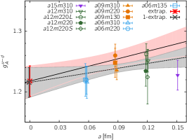
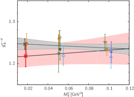
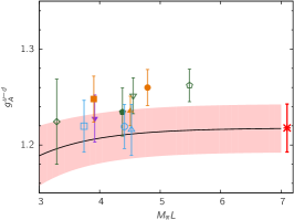
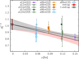
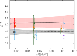
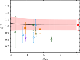
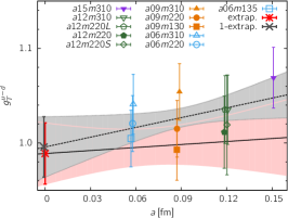
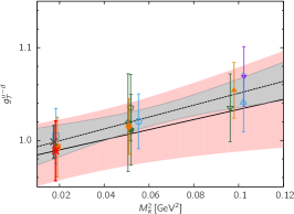
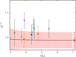
Figure 2: The 11-point CCFV fit using Eq. (12) to the data for the renormalized isovector charges $g_{A}^{u-d}$, $g_{S}^{u-d}$, and $g_{T}^{u-d}$ in the $\overline{{\rm MS}}$ scheme at 2 GeV. The result of the simultaneous extrapolation to the physical point defined by $a\rightarrow 0$, $M_{\pi}\rightarrow M_{\pi^{0}}^{{\rm phys}}=135$ MeV and $M_{\pi}L\rightarrow\infty$ are marked by a red star. The pink error band in each panel is the result of the simultaneous fit but shown as a function of a single variable. The overlay in the left (middle) panels with the dashed line within the grey band is the fit to the data versus $a$ ($M_{\pi}^{2}$), i.e., neglecting dependence on the other two variables. The symbols used to plot the data are defined in the left panels.

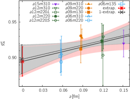
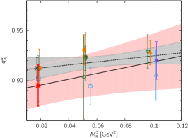
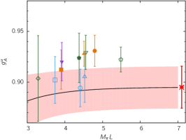
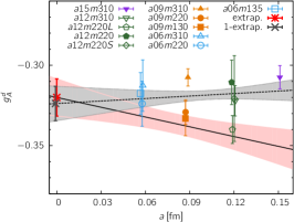
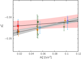
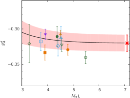
Figure 3: The 11-point CCFV fit using Eq. (12) to the connected data for the flavor diagonal charges $g_{A}^{u}$ and $g_{A}^{d}$ renormalized in the $\overline{{\rm MS}}$ scheme at 2 GeV. Only the data for $g_{A}^{u}$ show a notable dependence on the lattice spacing $a$. The rest is the same as in Fig. 2.

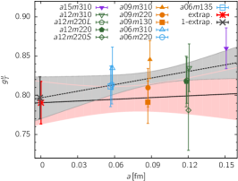
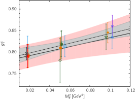
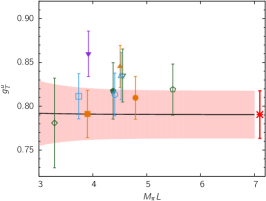
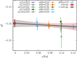
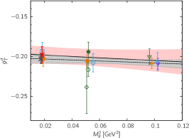
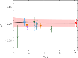
Figure 4: The 11-point CCFV fit using Eq. (12) to the connected data for the flavor diagonal charges $g_{T}^{u}$ and $g_{T}^{d}$ renormalized in the $\overline{{\rm MS}}$ scheme at 2 GeV. Only the data for $g_{T}^{u}$ show a notable dependence on $M_{\pi}$. The rest is the same as in Fig. 2.

Results of the 11-point, 10-point, and $10^{\ast}$-point fits to the connected contributions to the flavor-diagonal charges $g_{A,T}^{u,d}$, using the isovector renormalization factor $Z_{A,T}^{\rm isovector}$, respectively, are given in Table 7. Their behavior versus the lattice spacing and the pion mass is shown in Figs. 3 and 4 using the 11-point fits, again with $c_{3}^{\rm log}=0$ in the ansatz given in Eq. (12). The data exhibit the following features:

• The noticeable variation in the axial charges is in $g_{A}^{u}$ versus $a$ which carries over to $g_{A}^{u-d}$.

• The flavor diagonal charges $g_{T}^{u,d}$ show little variation except for the small dependence of $g_{T}^{u}$ on $M_{\pi}^{2}$ which carries over to $g_{T}^{u-d}$.

Our final results from the 11-point fits for the connected parts of the flavor diagonal charges for the proton are

$$g_{A}^{u,{\rm conn}} =0.895(21)\qquad\ g_{A}^{d,{\rm conn}}=-0.320(12)\,,$$

$$g_{T}^{u,{\rm conn}} =0.790(27)\qquad\ g_{T}^{d,{\rm conn}}=-0.198(10)\,.$$ (14)

Estimates for the neutron are given by the $u\leftrightarrow d$ interchange.

We again remind the reader that the disconnected contributions for the flavor diagonal axial charges are $O(15\%)$ and will be discussed elsewhere. The disconnected contribution to $g_{T}^{u+d}$ is small (comparable to the statistical errors) and $Z_{T}^{u-d}\approx Z_{T}^{u+d}$. Thus, the results for $g_{T}^{u,d}$ and $g_{T}^{u+d}$ are a good approximation to the total contribution. The new estimates given here supersede the values presented in Refs. Bhattacharya et al. (2015a, b).

	$c_{1}$	$c_{2}$	$c_{3}$	$c_{4}$	$g_{\Gamma}$
		fm-1	GeV-2	GeV-2
$g_{A}^{u-d}$	1.21(3)	0.41(26)	0.18(33)	$-$32(19)	1.218(25)
$g_{S}^{u-d}$	1.02(1)	$-$1.57(75)	0.22(1.12)	24(54)	1.022(80)
$g_{T}^{u-d}$	0.98(3)	0.11(38)	0.55(45)	5(29)	0.989(32)

Table 8: Values of the fit parameters in the CCFV ansatz defined in Eq. (12) with $c_{3}^{\rm log}=0$. The results are given for the 11-point fit used to extract the three isovector charges.

VI Assessing additional error due to CCFV fit ansatz

In this section we reassess the estimation of errors from various sources and provide an additional systematic uncertainty in the isovector charges due to using a CCFV ansatz with only the leading order correction terms. We first briefly review the systematics that are already addressed in our analysis leading to the results in Eq. (13):

• Statistical and excited-state contamination (SESC): Errors from these two sources are jointly estimated in the 2- and $3^{\ast}$ state fits. The 2- and $3^{\ast}$ state fits for $g_{A}^{u-d}$ and $g_{T}^{u-d}$ give overlapping results and in most cases the error estimates from the quoted $3^{\ast}$-state fits are larger. For $g_{S}^{u-d}$, we compare the 2- and $2^{\ast}$-state fits. Based on these comparisons, an estimate of the magnitude of possible residual ESC is given in the first row of Table 9 for all three charges.

• Uncertainty in the determination of the renormalization constants $Z_{\Gamma}$: The results for the $Z$’s and an estimate of the possible uncertainty presented in Ref. Bhattacharya et al. (2016) have not changed. These are reproduced in Tables 5 and 9, respectively. With the increase in statistical precision of the bare charges, the uncertainty in the $Z_{\Gamma}$ is now a significant fraction of the total uncertainty in $g_{A,S,T}^{u-d}$.

• Residual uncertainties due to the three systematics, extrapolations to $a\to 0$ and $M_{\pi}L\to\infty$ and the variation with $M_{\pi}$. Estimates of errors in the simultaneous CCFV fit using the lowest order corrections (see Eq. (12)) are given in rows 3–5 in Table 9. These are, in most cases, judged to be small because the variation with respect to the three variables, displayed in Fig. 2, is small. With increased statistics and the second physical mass ensemble, $a06m135$, our confidence in the CCFV fits and the error estimates obtained with keeping only the lowest-order corrections in each variable has increased significantly. The exception is the dependence of $g_{S}^{u-d}$ on $a$ as highlighted by the dependence of the extrapolated value on whether the $a15m310$ point is included (11-point fit) or excluded (10-point fit).

Adding the guesstimates for these five systematic uncertainties, given in rows 1–5, in quadrature, leads to an error estimate given in the sixth row in Table 9. This is consistent with the errors quoted in Eq. (13) and reproduced in the seventh row of Table 9. We, therefore, regard the fits and the error estimates given in Eq. (13) as adequately capturing the uncertainty due to the five systematics discussed above.

The $\chi^{2}/{\rm d.o.f.}$ of all four fits for the axial and tensor charges given in Table 6 are already very small. Therefore, adding higher order terms to the ansatz is not justified as per the Akaike Information Criterion Akaike (1974). Nevertheless, to be conservative, we quote an additional systematic uncertainty due to the truncation of the CCFV fit ansatz at the leading order in each of the three variables, by examining the variation in the data in Fig. 2.

For $g^{u-d}_{A}$, the key reason for the difference between our extrapolated value and the experimental results are the data on the $a\approx 0.06$ fm lattices. As discussed in Sec. VII, an extrapolation in $a$ with and without these ensembles gives $g^{u-d}_{A}=1.218(25)$ and $g^{u-d}_{A}=1.245(42)$, respectively. The difference, $0.03$, is roughly half the total spread between the fourteen values of $g^{u-d}_{A}$ given in Table 6. We, therefore, quote $0.03$ as the additional uncertainty due to the truncation of the fit ansatz.

The dominant variation in $g^{u-d}_{S}$ is again versus $a$, and, as stated above, the result depends on whether the $a15m310$ point is included in the fit. We, therefore, take half the difference, $0.06$, between the 11-point and 10-point fit values as the additional systematic uncertainty. One gets a similar estimate by taking the difference in the fit value at $a=0.06$ fm and $a=0$. For $g^{u-d}_{T}$, the largest variation is versus $M_{\pi}^{2}$. Since we have data from two ensembles at $M_{\pi}\approx 135$ MeV that anchor the chiral fit, we take half the difference in the fit values at $M_{\pi}=135$ and $220$ MeV as the estimate of the additional systematic uncertainty.

These error estimates, rounded up to two decimal places, are given in the last row of Table 9. Including them as a second systematic error, our final results for the isovector charges in the $\overline{\rm MS}$ scheme at 2 GeV are:

$$g_{A}^{u-d} =1.218(25)(30)\,,$$

$$g_{S}^{u-d} =1.022(80)(60)\,,$$

$$g_{T}^{u-d} =0.989(32)(10)\,.$$ (15)

Similar estimates of possible extrapolation uncertainty apply also to results for the connected contributions to the flavor diagonal charges presented in Eq. (14). Their final analysis, including disconnected contributions, will be presented in a separate publication.

Error From	$g_{A}^{u-d}$	$g_{S}^{u-d}$	$g_{T}^{u-d}$
SESC	$0.02$ $\Uparrow$	$0.03$ $\Uparrow$	$0.01$ $\Downarrow$
$Z$	$0.01$ $\Downarrow$	$0.04$ $\Uparrow$	$0.03$ $\Downarrow$
$a$	$0.02$ $\Downarrow$	$0.04$ $\Uparrow$	$0.01$ $\Downarrow$
Chiral	$0.01$ $\Uparrow$	$0.01$ $\Downarrow$	$0.02$ $\Downarrow$
Finite volume	$0.01$ $\Uparrow$	$0.01$ $\Uparrow$	$0.01$ $\Uparrow$
Guesstimate error	$0.033$	$0.066$	$0.04$
Error quoted	$0.025$	$0.080$	$0.032$
Fit ansatz	$0.03$	$0.06$	$0.01$

Table 9: Estimates of the error budget for the three isovector charges due to each of the five systematic effects described in the text. The symbols $\Uparrow$ and $\Downarrow$ indicate the direction in which a given systematic is observed to drive the central value obtained from the 11-point fit. The sixth row gives a guesstimate of error obtained by combining these five systematics in quadrature. This guesstimate is consistent with the actual errors obtained from the 11-point fit and quoted in Eq. 13 and reproduced in the seventh row. The last row gives the additional systematic error assigned to account for possible uncertainty due to the using the CCFV fit ansatz with just the lowest order correction terms as described in the text.

Our new estimate $g_{S}^{u-d}=1.022(80)(60)$ is in very good agreement with $g_{S}^{u-d}=1.02(8)(7)$ obtained by Gonzalez-Alonso and Camalich González-Alonso and Martin Camalich (2014) using the conserved vector current (CVC) relation $g_{S}/g_{V}=(M_{N}-M_{P})^{\rm QCD}/(m_{d}-m_{u})^{\rm QCD}$ with the FLAG lattice-QCD estimates The Flavor Lattice Averaging Group (2016) (FLAG) for the two quantities on the right hand side. The superscript QCD denotes that the results are in a theory with just QCD, i.e., neglecting electromagnetic corrections. Using CVC in reverse, our predictions for $(M_{N}-M_{P})^{\rm QCD}$, using lattice QCD estimates for $m_{u}$ and $m_{d}$, are given in Table 10. The uncertainty in these estimates is dominated by that in $g_{S}^{u-d}$.

$M_{N}-M_{P}$	$N_{f}$	$\{m_{d},m_{u}\}^{\rm QCD}$
(MeV)	Flavors	(MeV)
$2.58(32)$	2+1	$m_{d}=4.68(14)(7),m_{u}=2.16(9)(7)$ The Flavor Lattice Averaging Group (2016) (FLAG)
$2.73(44)$	2+1+1	$m_{d}=5.03(26),m_{u}=2.36(24)$ The Flavor Lattice Averaging Group (2016) (FLAG)
$2.41(27)$	2+1	$m_{d}-m_{u}=2.41(6)(4)(9)$ Fodor et al. (2016)
$2.63(27)$	2+1+1	$m_{d}=4.690(54),m_{u}=2.118(38)$ Bazavov et al. (2018)

Table 10: Results for the mass difference $(M_{N}-M_{P})^{\rm QCD}$ obtained using the CVC relation with our estimate $g_{S}^{u-d}=1.022(80)(60)$ and lattice results for the up and down quark masses from the FLAG review The Flavor Lattice Averaging Group (2016) (FLAG) and recent results Fodor et al. (2016); Bazavov et al. (2018).

VII Comparison with Previous Work

A summary of lattice results for the three isovector charges for $N_{f}=2$-, 2+1- and 2+1+1-flavors is shown in Figs. 5, 6 and 7. They show the steady improvement in results from lattice QCD. In this section we compare our results with two calculations published after the analysis and the comparison presented in Ref. Bhattacharya et al. (2016), and that include data from physical pion mass ensembles. These are the ETMC Alexandrou et al. (2017b, a, c) and CalLat results Chang et al. (2018).

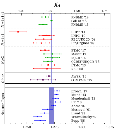
Figure 5: A summary of results for the axial isovector charge, $g_{A}^{u-d}$, for $N_{f}=2$- 2+1- and 2+1+1-flavors. Note the much finer x-axis scale for the plot showing experimental results for $g_{A}^{u-d}$. The lattice results (top panel) are from: PNDME’18 (this work); PNDME’16 Bhattacharya et al. (2016); CalLat’18 Chang et al. (2018); LHPC’14 Green et al. (2014); LHPC’10 Bratt et al. (2010); RBC/UKQCD’08 Lin et al. (2008); Lin/Orginos’07 Lin and Orginos (2009); ETMC’17 Alexandrou et al. (2017b, c); Mainz’17 Capitani et al. (2017) RQCD’14 Bali et al. (2015); QCDSF/UKQCD’13 Horsley et al. (2014); ETMC’15 Abdel-Rehim et al. (2015) and RBC’08 Yamazaki et al. (2008). Phenomenological and other experimental results (middle panel) are from: AWSR’16 Beane and Klco (2016) and COMPASS’15 Adolph et al. (2016). The results from neutron decay experiments (bottom panel) have been taken from: Brown’17 Brown et al. (2018); Mund’13 Mund et al. (2013); Mendenhall’12 Mendenhall et al. (2013); Liu’10 Liu et al. (2010); Abele’02 Abele et al. (2002); Mostovoi’01 Mostovoi et al. (2001); Liaud’97 Liaud et al. (1997); Yerozolimsky’97 Erozolimsky et al. (1997) and Bopp’86 Bopp et al. (1986). The lattice-QCD estimates in red indicate that estimates of excited-state contamination, or discretization errors, or chiral extrapolation were not presented. When available, systematic errors have been added to statistical ones as outer error bars marked with dashed lines.

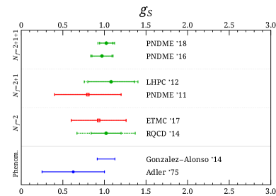
Figure 6: A summary of results for the isovector scalar charge, $g_{S}^{u-d}$, for $N_{f}=2$- 2+1- and 2+1+1-flavors. The lattice results are from: PNDME’18 (this work); PNDME’16 Bhattacharya et al. (2016); LHPC’12 Green et al. (2012); PNDME’11 Bhattacharya et al. (2012); ETMC’17 Alexandrou et al. (2017a) and RQCD’14 Bali et al. (2015). The estimates based on the conserved vector current and phenomenology are taken from Gonzalez-Alonso’14 González-Alonso and Martin Camalich (2014) and Adler’75 Adler et al. (1975). The rest is the same as in Fig. 5.

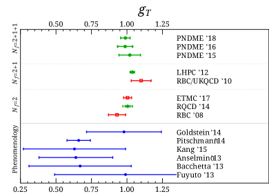
Figure 7: A summary of results for the isovector tensor charge, $g_{T}^{u-d}$, for $N_{f}=2$- 2+1- and 2+1+1-flavors. The lattice and phenomenology results quoted from: PNDME’18 (this work); PNDME’16 Bhattacharya et al. (2016); PNDME’15 Bhattacharya et al. (2015a) LHPC’12 Green et al. (2012); RBC/UKQCD’10 Aoki et al. (2010); ETMC’17 Alexandrou et al. (2017a); RQCD’14 Bali et al. (2015) and RBC’08 Yamazaki et al. (2008). The phenomenological estimates are taken from the following sources: Kang’15 Kang et al. (2016); Goldstein’14 Goldstein et al. (2014); Pitschmann’14 Pitschmann et al. (2015); Anselmino’13 Anselmino et al. (2013); Bacchetta’13 Bacchetta et al. (2013) and Fuyuto’13 Fuyuto et al. (2013). Rest same as in Fig. 5.

The ETMC results $g_{A}^{u-d}=1.212(40)$, $g_{S}^{u-d}=0.93(33)$ and $g_{T}^{u-d}=1.004(28)$ Alexandrou et al. (2017b, a, c) were obtained from a single physical mass ensemble generated with 2-flavors of maximally twisted mass fermions with a clover term at $a=0.0938(4)$ fm, $M_{\pi}=130.5(4)$ MeV and $M_{\pi}L=2.98$. Assuming that the number of quark flavors and finite volume corrections do not make a significant difference, one could compare them against our results from the $a09m130W$ ensemble with similar lattice parameters: $g_{A}^{u-d}=1.249(21)$, $g_{S}^{u-d}=0.952(74)$ and $g_{T}^{u-d}=1.011(30)$. We remind the reader that this comparison is at best qualitative since estimates from different lattice actions are only expected to agree in the continuum limit.

Based on the trends observed in our CCFV fits shown in Figs. 2–4, we speculate where one may expect to see a difference due to the lack of a continuum extrapolation in the ETMC results. The quantities that exhibit a significant slope versus $a$ are $g_{A}^{u-d}$ and $g_{S}^{u-d}$. Again, under the assumptions stated above, we would expect ETMC values $g_{A}^{u-d}=1.212(40)$ to be larger and $g_{S}^{u-d}=0.93(33)$ to be smaller than our extrapolated values given in Eq. (13). We find that the scalar charge (ignoring the large error) fits the expected pattern, but the axial charge does not.

We also point out that the ETMC error estimates are taken from a single ensemble and a single value of the source-sink separation using the plateau method. Our results from the comparable calculation on the $a09m130W$ ensemble with $\tau=14$ (see Figs. 10 and 16 and results in Table 13), have much smaller errors.

The more detailed comparison we make is against the CalLat result $g_{A}^{u-d}=1.271(13)$ Chang et al. (2018) that agrees with the latest experimental average, $g_{A}^{u-d}=1.2766(20)$. The important question is, since the CalLat calculations were also done using the same 2+1+1-flavor HISQ ensembles, why are the two results, after CCFV fits, different?

To understand why the results can be different, we first review the notable differences between the two calculations. CalLat uses (i) Möbius domain wall versus clover for the valence quark action. This means that their discretization errors start at $a^{2}$ versus $a$ for PNDME. They also have no uncertainty due to the renormalization factor since $Z_{A}/Z_{V}=1$ for the Möbius domain wall on HISQ formalism. (ii) They use gradient flow smearing with $t_{gf}/a=1$ versus one HYP smearing to smooth high frequency fluctuations in the gauge configurations. This can impact the size of statistical errors. (iii) Different construction of the sequential propagator. CalLat inserts a zero-momentum projected axial current simultaneously at all time slices on the lattice to construct the sequential propagator. Their data are, therefore, for the sum of contributions from insertions on all time slices on the lattice, i.e., including contact terms and insertion on time slices outside the interval between the source and the sink. CalLat fits this summed three-point function versus only the source-sink separation $\tau$ using the 2-state fit ansatz. (iv) The ranges of $\tau$ for which the data have the maximum weight in the respective n-state fits are very different in the two calculations. The CalLat results are obtained from data at much smaller values of $\tau$, which accounts for the smaller error estimates in the data for $g_{A}^{u-d}$. (v) CalLat analyze the coarser $a\approx 0.15$, $0.12$ and $0.09$ fm ensembles. At $a\approx 0.15$ fm, we can only analyze the $a15m310$ ensemble due to the presence of exceptional configurations in the clover-on-HISQ formulation at lighter pion masses. On the other hand, computing resources have so far limited CalLat from analyzing the three fine $a\approx 0.06$ fm and the physical mass $a09m130$ ensembles.

A combination of these factors could easily explain the $\approx 5\%$ difference in the final values. The surprising result, shown in Table 11, is that estimates on the seven ensembles analyzed by both collaborations are consistent and do not show a systematic difference. (Note again that results from two different lattice formulations are not, a priori, expected to agree at finite $a$.) These data suggest that differences at the $1\sigma$ level (see also our analysis in Table 9) are conspiring to produce a 5% difference in the extrapolated value. Thus, one should look for differences in the details of the CCFV fit.

We first examine the extrapolation in $a$. A CCFV fit keeping our data from only the eight $a\approx 0.15$, $0.12$ and $0.09$ fm ensembles gives a larger value, $g_{A}^{u-d}=1.245(42)$, since the sign of the slope versus $a$ changes sign as is apparent from the data shown in the top three panels of Fig. 2. Thus the three $a\approx 0.06$ fm ensembles play an important role in our continuum extrapolation.

Our initial concern was possible underestimation of statistical errors in results from the $a\approx 0.06$ fm lattices. This prompted us to analyze three crucial ensembles, $a09m130$, $a06m310$ and $a06m220$, a second time with different smearing sizes and different random selection of source points. The consistency between the pairs of data points on these ensembles suggests that statistical fluctuations are not a likely explanation for the size of the undershoot in $g_{A}^{u-d}$. The possibility that these ensembles are not large enough to have adequately explored the phase space of the functional integral, and the results are possibly biased, can only be checked with the generation and analysis of additional lattices.

The chiral fits are also different in detail. In our data, the errors in the points at $M_{\pi}\approx 310$, 220 and 130 MeV are similar, consequently all points contribute with similar weight in the fits. The errors in the CalLat data from the two physical mass ensembles $a15m130$ and $a12m130$ are much larger and the fits are predominately weighted by the data at the heavier masses $M_{\pi}\approx 400$, 350 310 and 220 MeV. Also, CalLat finds a significant change in the value between the $M_{\pi}\approx\{400,\ 350,\ 310\}$  MeV and $M_{\pi}\approx 220$ MeV points, and this concerted change, well within $1\sigma$ errors in individual points, produces a larger dependence on $M_{\pi}$. In other words, it is the uniformly smaller values on the $M_{\pi}\approx\{400,\ 350,\ 310\}$ MeV ensembles compared to the data at $M_{\pi}\approx 220$ MeV that makes the CalLat chiral fits different and the final value of $g_{A}^{u-d}$ larger.

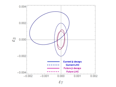
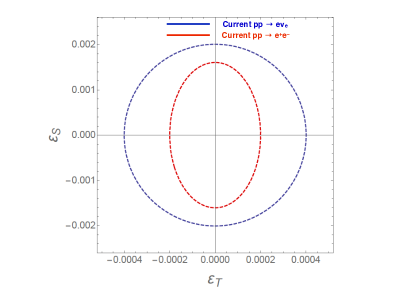
Figure 8: Current and projected $90\%$ C.L. constraints on $\epsilon_{S}$ and $\epsilon_{T}$ defined at 2 GeV in the $\overline{MS}$ scheme. (Left) The beta-decay constraints are obtained from the recent review article Ref. González-Alonso et al. (2018). The current and future LHC bounds are obtained from the analysis of the $pp\to e+MET+X$. We have used the ATLAS results Aaboud et al. (2018), at $\sqrt{s}=13$ TeV and integrated luminosity of 36 fb^-1. We find that the strongest bound comes from the cumulative distribution with a cut on the transverse mass at 2 TeV. The projected future LHC bounds are obtained by assuming that no events are observed at transverse mass greater than 3 TeV with an integrated luminosity of 300 fb^-1. (Right) Comparison of current LHC bounds from $pp\to e+MET+X$ versus $pp\to e^{+}e^{-}+X$.

To summarize, the difference between our and CalLat results comes from the chiral fit and the continuum extrapolation. The difference in the chiral fit is a consequence of the “jump” in the CalLat data between $M_{\pi}=\{400,\ 350,\ 310\}$ and the $220$ MeV data. The CalLat data at $M_{\pi}\approx 130$ MeV do not contribute much to the fit because of the much larger errors. We do not see a similar jump between our $M_{\pi}\approx 310$ and $220$ MeV or between the 220 and the 130 MeV data as is evident from Fig. 2. Also, our four data points at $M_{\pi}\approx 310$ MeV show a larger spread. The difference in the continuum extrapolation is driven by the smaller estimates on all three fine $a\approx 0.06$ fm ensembles that we have analyzed. Unfortunately, neither of these two differences in the fits can be resolved with the current data, especially since the data on 7 ensembles, shown in Table 11, agree within $1\sigma$. Our two conclusions are: (i) figuring out why the $a\approx 0.06$ fm ensembles give smaller estimates is crucial to understanding the difference, and (ii) with present data, a total error estimate of $\approx 5\%$ in $g_{A}^{u-d}$ is realistic.

	This Work	CalLat
$a15m310$	1.228(25)	1.215(12)
$a12m310$	1.251(19)	1.214(13)
$a12m220S$	1.224(44)	1.272(28)
$a12m220$	1.234(25)	1.259(15)
$a12m220L$	1.262(17)	1.252(21)
$a09m310$	1.235(15)	1.236(11)
$a09m220$	1.260(19)	1.253(09)

Table 11: The data for the renormalized axial charge $g_{A}^{u-d}$ for the proton on the seven 2+1+1-flavor HISQ ensembles that have been analyzed by us and the CalLat collaboration Chang et al. (2018). The results are consistent within $1\sigma$ in most cases.

Even with the high statistics calculation presented here, the statistical and ESC errors in the calculation of the scalar charge are between 5%–15% on individual ensembles. As a result, the error after the continuum extrapolation is about $10\%$. Over time, results for $g_{S}^{u-d}$, presented in Fig. 6, do show significant reduction in the error with improved higher-statistics calculations.

The variation of the tensor charge $g_{T}^{u-d}$ with $a$ or $M_{\pi}$ or $M_{\pi}L$ is small. As a result, the lattice estimates have been stable over time as shown in Fig. 7. The first error estimate in our result, $g_{T}^{u-d}=0.989(32)(10)$, is now dominated by the error in $Z_{T}$.

VIII Constraining new physics using precision beta decay measurements

Nonstandard scalar and tensor charged-current interactions are parametrized by the dimensionless couplings $\epsilon_{S,T}$ Bhattacharya et al. (2012); Cirigliano et al. (2013):

$${\cal L}_{\rm CC} = -\frac{G_{F}^{(0)}V_{ud}}{\sqrt{2}}\ \Big{[}\ \epsilon_{S}\ \bar{e}(1-\gamma_{5})\nu_{\ell}\cdot\bar{u}d$$ (16)

$$+ \epsilon_{T}\ \bar{e}\sigma_{\mu\nu}(1-\gamma_{5})\nu_{\ell}\cdot\bar{u}\sigma^{\mu\nu}(1-\gamma_{5})d\Big{]}~{}.$$

These couplings can be constrained by a combination of low energy precision beta-decay measurements (of the pion, neutron, and nuclei) combined with our results for the isovector charges $g_{S}^{\rm u-d}$ and $g_{T}^{\rm u-d}$, as well at the Large Hadron Collider (LHC) through the reaction $pp\to e\nu+X$ and $pp\to e^{+}e^{-}+X$. The LHC constraint is valid provided the mediator of the new interaction is heavier than a few TeV.

In Fig. 8 (left) we show current and projected bounds on $\{\epsilon_{S},\epsilon_{T}\}$ defined at 2 GeV in the $\overline{MS}$ scheme. The beta decays constraints are obtained from the recent review article Ref. González-Alonso et al. (2018). The current analysis includes all existing neutron and nuclear decay measurements, while the future projection assumes measurements of the various decay correlations with fractional uncertainty of $0.1\%$, the Fierz interference term at the $10^{-3}$ level, and neutron lifetime with uncertainty $\delta\tau_{n}=0.1s$. The current LHC bounds are obtained from the analysis of the $pp\to e+MET+X$, where $MET$ stands for missing transverse energy. We have used the ATLAS results Aaboud et al. (2018), at $\sqrt{s}=13$ TeV and integrated luminosity of 36 fb^-1. We find that the strongest bound comes by the cumulative distribution with a cut on the transverse mass at 2 TeV. The projected future LHC bounds are obtained by assuming that no events are observed at transverse mass greater than 3 TeV with an integrated luminosity of 300 fb^-1.

The LHC bounds become tighter on the inclusion of $Z$-like mediated process $pp\to e^{+}e^{-}+X$. As shown in Fig. 8 (right), including both $W$-like and $Z$-like mediated processes, the current LHC bounds are comparable to future low energy ones, motivating more precise low energy experiments. In this analysis we have neglected the NLO QCD corrections Alioli et al. (2018), which would further strengthen the LHC bounds by $O(10\%)$. Similar bounds are obtained using the CMS data Sirunyan et al. (2018a, b).

IX Conclusions

We have presented a high-statistics study of the isovector and flavor-diagonal charges of the nucleon using clover-on-HISQ lattice QCD formulation. By using the truncated solver with bias correction error-reduction technique with the multigrid solver, we have significantly improved the statistical precision of the data. Also, we show stability in the isolation and mitigation of excited-state contamination by keeping up to three states in the analysis of data at multiple values of source-sink separation $\mathop{\tau}\nolimits$. Together, these two improvements allow us to demonstrate that the excited-state contamination in the axial and the tensor channels has been reduced to the 1%–2% level. The high-statistics analysis of eleven ensembles covering the range 0.15–0.06 fm in the lattice spacing, $M_{\pi}=$ 135–320 MeV in the pion mass, and $M_{\pi}L=$ 3.3–5.5 in the lattice size allowed us to analyze the three systematic uncertainties due to lattice discretization, dependence on the quark mass and finite lattice size, by making a simultaneous fit in the three variables $a$, $M_{\pi}^{2}$ and $M_{\pi}L$. Data from the two physical mass ensembles, $a09m130$ and $a06m135$, anchor the improved chiral fit. Our final estimates for the isovector charges are given in Eq. (15).

One of the largest sources of uncertainty now is from the calculation of the renormalization constants for the quark bilinear operators. These are calculated nonperturbatively in the RI-sMOM scheme over a range of values of the scale $Q^{2}$. As discussed in Ref. Bhattacharya et al. (2016), the dominant systematics in the calculation of the $Z$’s comes from the breaking of the rotational symmetry on the lattice and the 2-loop perturbative matching between the RI-sMOM and the $\overline{\text{MS}}$ schemes.

Our estimate $g_{A}^{u-d}=1.218(25)(30)$ is about $1.5\sigma$ (about $5\%$) below the experimental value $g_{A}/g_{V}=1.2766(20)$. Such low values are typical of most lattice QCD calculations. The recent calculation by the CalLat collaboration, also using the 2+1+1-flavor HISQ ensembles, gives $g_{A}^{u-d}=1.271(13)$ Chang et al. (2018). A detailed comparison between the two calculations is presented in Sec VII. We show in Table 11 that results from seven ensembles, which have been analyzed by both collaborations, agree within $1\sigma$ uncertainty. Our analysis indicates that the majority of the difference comes from the chiral and continuum extrapolations, with $1\sigma$ differences in individual points getting amplified. Given that CalLat have not analyzed the fine $0.06$ fm ensembles and their data on the two physical pion mass ensembles, $a15m130$ and $a12m130$ have much larger errors and do not contribute significantly to their chiral fit, we conclude that our error estimate is more realistic. Further work is, therefore, required to resolve the difference between the two results.

Our results for the isovector scalar and tensor charges, $g_{S}^{u-d}=1.022(80)(60)$ and $g_{T}^{u-d}=0.989(32)(10)$, have achieved the target accuracy of 10% needed to put bounds on scalar and tensor interactions, $\epsilon_{S}$ and $\epsilon_{T}$, arising at the TeV scale when combined with experimental measurements of $b$ and $b_{\nu}$ parameters in neutron decay experiments with $10^{-3}$ sensitivity Bhattacharya et al. (2012). In Sec. VIII, we update the constraints on $\epsilon_{S}$ and $\epsilon_{T}$ from both low energy experiments combined with our new lattice results on $g_{S}^{u-d}$ and $g_{T}^{u-d}$, and from the ATLAS and the CMS experiments at the LHC. We find that the constraints from low energy experiments combined with matrix elements from lattice QCD are comparable to those from the LHC.

For the tensor charges, we find that the dependence on the lattice size, the lattice spacing and the light-quark mass is small, and the simultaneous fit in these three variables, keeping just the lowest-order corrections, has improved over that presented in Ref. Bhattacharya et al. (2015a).

We have also updated our estimates for the connected parts of the flavor-diagonal charges. For the tensor charges, the contribution of the disconnected diagram is consistent with zero Bhattacharya et al. (2015a, b), so the connected contribution, $g_{T}^{u}=0.790(27)$ and $g_{T}^{d}=-0.198(10)$ for the proton, is a good approximation to the full result that will be discussed elsewhere.

The extraction of the scalar charge of the proton has larger uncertainty. The statistical errors in the lattice data for $g_{S}^{u-d}(a,M_{\pi},M_{\pi}L)$ are 3–5 times larger than those in $g_{T}^{u-d}(a,M_{\pi},M_{\pi}L)$, and the data show significant dependence on the lattice spacing $a$ and a weaker dependence on the pion mass $M_{\pi}$. Our estimate, $g_{S}^{u-d}=1.022(80)(60)$, is in very good agreement with the estimate $g_{S}^{u-d}=1.02(8)(7)$ obtained using the CVC relation $g_{S}/g_{V}=(M_{N}-M_{P})^{\rm QCD}/(m_{d}-m_{u})^{\rm QCD}$ in Ref. González-Alonso and Martin Camalich (2014). In Table 10, we used our new estimate to update the results for the mass difference $(M_{N}-M_{P})^{\rm QCD}$ obtained by using the CVC relation. Taking the recent 2+1 flavor value $m_{d}-m_{u}=2.41(6)(4)(9)$ MeV from the BMW collaboration Fodor et al. (2016) gives $(M_{N}-M_{P})^{\rm 2+1QCD}=2.41(27)$ MeV, while the 2+1+1-flavor estimates $m_{u}=2.118(38)$ MeV and $m_{d}=4.690(54)$ MeV from the MILC/Fermilab/TUMQCD collaboration Bazavov et al. (2018) give $(M_{N}-M_{P})^{\rm 2+1+1QCD}=2.63(27)$ MeV.

Appendix A ESC in the extraction of the isovector charges

In this Appendix, we first present the masses and amplitudes obtained from fits to the 2-point function using the spectral decomposition, Eq. (9), in Table LABEL:tab:2ptmulti. These are used as inputs in the fits to the 3-point functions using Eq. (10). We then give in Tables 13 and 14 the results of $2^{\ast}$-, 2- and $3^{\ast}$-state fits used to control the ESC in the extraction of the isovector and the connected contribution to the isoscalar axial, scalar and tensor charges for the fourteen calculations. The data and the $2^{\ast}$-, 2- and $3^{\ast}$-state fits are shown in Figs. 9–17. In each case, we compare the $2^{\ast}$ fit on data from two source-sink separations with $\tau\approx 1$ fm with the $2$- or $3^{\ast}$-state fit using data from multiple values of $\tau$.

Table 12: Results of 2-, 3- and 4-state fits to the two-point correlation function data for the fourteen calculations. The first column specifies the parameters, {$N_{\text{2pt}}$, $t_{\text{min}}$– $t_{\text{max}}$}, where $N_{\text{2pt}}$ is number of states used in the fits to the two-point correlators, and $[t_{\text{min}},t_{\text{max}}]$ is the fit interval in lattice units. The following columns give the nucleon ground state amplitude $\mathcal{A}_{0}^{2}$ and mass $aM_{0}$, followed by the ratio of the excited state amplitudes $r_{i}=(\mathcal{A}_{i}/\mathcal{A}_{0})^{2}$, and the mass gaps $a\Delta M_{i}=a(M_{i}-M_{i-1})$. For each ensemble, the first row gives the values of the priors used in the final 3- and 4-state fits.

	$\mathcal{A}_{0}^{2}$	$aM_{0}$	$r_{1}$	$a\Delta M_{1}$	$r_{2}$	$a\Delta M_{2}$	$r_{3}$	$a\Delta M_{3}$	$\chi^{2}/\text{d.o.f}$
	$a15m310$ Smearing $\sigma=4.2$
Priors			0.5(3)	0.7(4)	0.3(2)	0.4(2)	0.3(2)	0.4(2)
{2,3–10}	$8.76(17)\times 10^{-9}$	0.833(003)	0.750(279)	0.926(194)					1.304
{3,1–10}	$8.61(09)\times 10^{-9}$	0.831(002)	0.479(013)	0.769(026)	0.251(013)	0.316(047)			0.892
{4,1–10}	$8.58(10)\times 10^{-9}$	0.830(002)	0.420(042)	0.729(048)	0.241(011)	0.281(034)	0.084(061)	0.366(016)	1.146
	$a12m310$ Smearing $\sigma=5.5$
Priors			0.15(10)	0.4(2)	0.8(6)	0.6(3)	0.6(4)	0.4(2)
{2,3–15}	$6.86(11)\times 10^{-11}$	0.671(2)	1.011(186)	0.837(098)					0.916
{3,2–15}	$6.78(10)\times 10^{-11}$	0.670(2)	0.143(028)	0.450(038)	1.137(063)	0.563(075)			0.747
{4,2–15}	$6.75(10)\times 10^{-11}$	0.669(2)	0.137(030)	0.420(037)	0.732(038)	0.500(066)	0.518(066)	0.396(023)	0.738
	$a12m220S$ Smearing $\sigma=5.5$
Priors			0.4(3)	0.3(2)	1.0(8)	0.8(4)	0.8(6)	0.4(2)
{2,4–15}	$5.69(51)\times 10^{-11}$	0.607(8)	0.681(086)	0.419(132)					0.124
{3,2–15}	$5.53(26)\times 10^{-11}$	0.605(4)	0.488(079)	0.310(036)	1.591(226)	0.968(110)			0.181
{4,2–15}	$5.46(32)\times 10^{-11}$	0.604(5)	0.525(095)	0.309(047)	0.994(167)	0.913(126)	0.853(130)	0.405(006)	0.136
	$a12m220$ Smearing $\sigma=5.5$
Priors			0.4(3)	0.3(2)	1.0(8)	0.8(4)	0.8(6)	0.4(2)
{2,4–15}	$6.09(18)\times 10^{-11}$	0.612(3)	0.832(303)	0.637(157)					0.285
{3,2–15}	$5.86(19)\times 10^{-11}$	0.608(3)	0.376(071)	0.386(056)	1.304(164)	0.770(128)			0.234
{4,2–15}	$5.83(18)\times 10^{-11}$	0.608(3)	0.365(131)	0.372(070)	0.801(071)	0.670(145)	0.631(124)	0.404(011)	0.254
	$a12m220L_{O}$ Smearing $\sigma=5.5$
Priors			0.4(3)	0.3(2)	1.0(8)	0.8(4)	0.8(6)	0.4(2)
{2,4–15}	$5.97(18)\times 10^{-11}$	0.612(3)	0.669(118)	0.529(100)					1.363
{3,2–15}	$5.75(22)\times 10^{-11}$	0.609(3)	0.400(067)	0.350(071)	1.461(171)	0.878(102)			0.885
{4,2–15}	$5.74(23)\times 10^{-11}$	0.609(3)	0.400(091)	0.349(085)	0.873(099)	0.775(117)	0.725(107)	0.405(010)	0.881
	$a12m220L$ Smearing $\sigma=5.5$
Priors			0.4(3)	0.3(2)	1.0(8)	0.8(4)	0.8(6)	0.4(2)
{2,4–15}	$6.14(11)\times 10^{-11}$	0.615(2)	0.825(165)	0.642(088)					0.216
{3,2–15}	$5.96(13)\times 10^{-11}$	0.613(2)	0.391(114)	0.420(082)	1.258(114)	0.759(105)			0.223
{4,2–15}	$5.94(14)\times 10^{-11}$	0.612(2)	0.371(152)	0.406(106)	0.763(064)	0.645(112)	0.611(083)	0.411(011)	0.233
	$\mathcal{A}_{0}^{2}$	$aM_{0}$	$r_{1}$	$a\Delta M_{1}$	$r_{2}$	$a\Delta M_{2}$	$r_{3}$	$a\Delta M_{3}$	$\chi^{2}/\text{d.o.f}$
	$a09m310$ Smearing $\sigma=7$
Priors			0.7(4)	0.40(25)	1.0(5)	0.70(35)	1.0(6)	0.5(3)
{2,4–18}	$3.64(04)\times 10^{-13}$	0.496(1)	0.924(052)	0.500(029)					1.438
{3,2–18}	$3.60(06)\times 10^{-13}$	0.495(1)	0.697(092)	0.432(044)	1.425(111)	0.810(086)			1.191
{4,2–18}	$3.60(06)\times 10^{-13}$	0.495(1)	0.702(140)	0.434(058)	0.854(051)	0.696(133)	0.807(129)	0.526(024)	1.146
	$a09m220$ Smearing $\sigma=7$
Priors			0.6(3)	0.30(15)	0.8(5)	0.4(2)	0.7(4)	0.4(2)
{2,5–20}	$3.02(06)\times 10^{-13}$	0.451(2)	0.937(067)	0.407(034)					0.466
{3,3–20}	$2.99(07)\times 10^{-13}$	0.450(2)	0.566(061)	0.329(036)	1.097(139)	0.453(061)			0.509
{4,3–20}	$2.97(07)\times 10^{-13}$	0.450(2)	0.529(076)	0.314(040)	0.723(074)	0.370(056)	0.591(098)	0.386(031)	0.502
	$a09m130$ Smearing $\sigma=5.5$
Priors			1.0(5)	0.20(15)	2.0(1.5)	0.6(3)	1.7(1.2)	0.4(2)
{2,6–20}	$8.92(51)\times 10^{-11}$	0.417(4)	1.322(083)	0.329(041)					0.727
{3,4–20}	$8.15(72)\times 10^{-11}$	0.412(5)	1.067(100)	0.244(043)	2.572(522)	0.666(079)			0.627
{4,4–20}	$8.21(71)\times 10^{-11}$	0.412(5)	1.104(089)	0.253(043)	1.924(389)	0.661(082)	1.771(242)	0.402(020)	0.597
	$a09m130W$ Smearing $\sigma=7.0$
Priors			0.7(4)	0.35(20)	0.7(5)	0.5(3)	1.0(6)	0.35(20)
{2,6–20}	$2.74(07)\times 10^{-13}$	0.422(2)	1.071(165)	0.415(052)					0.670
{3,4–20}	$2.70(06)\times 10^{-13}$	0.421(2)	0.794(076)	0.359(031)	0.857(214)	0.482(051)			0.533
{4,4–20}	$2.69(06)\times 10^{-13}$	0.421(2)	0.833(108)	0.356(039)	0.623(106)	0.538(051)	0.942(124)	0.367(021)	0.524
	$a06m310$ Smearing $\sigma=6.5$
Priors			1.0(5)	0.16(10)	2.4(1.5)	0.3(2)	2.2(1.5)	0.3(2)
{2,0–30}	$5.56(35)\times 10^{-12}$	0.326(3)	1.362(097)	0.199(026)					1.371
{3,7–30}	$5.46(39)\times 10^{-12}$	0.325(3)	0.936(109)	0.163(028)	3.368(597)	0.356(035)			1.268
{4,7–30}	$5.40(43)\times 10^{-12}$	0.325(3)	0.964(116)	0.161(031)	2.554(366)	0.338(037)	2.323(334)	0.276(042)	1.238
	$a06m310W$ Smearing $\sigma=12.0$
Priors			0.7(4)	0.3(2)	0.7(4)	0.3(2)	0.7(4)	0.3(2)
{2,6–25}	$1.34(04)\times 10^{-22}$	0.329(2)	1.229(252)	0.377(059)					1.488
{3,4–25}	$1.33(03)\times 10^{-22}$	0.328(1)	0.769(042)	0.317(031)	0.860(135)	0.293(061)			1.162
{4,4–25}	$1.31(04)\times 10^{-22}$	0.328(2)	0.646(084)	0.278(043)	0.685(102)	0.278(057)	0.655(136)	0.293(033)	1.150
	$a06m220$ Smearing $\sigma=5.5$
Priors			2.0(1.0)	0.25(20)	3.0(1.5)	0.3(2)	2.8(1.8)	0.3(2)
{2,0–30}	$1.08(04)\times 10^{-10}$	0.305(2)	2.900(348)	0.286(025)					1.774
{3,7–30}	$1.06(04)\times 10^{-10}$	0.304(2)	2.035(225)	0.249(019)	3.919(681)	0.342(021)			1.591
{4,7–30}	$1.05(04)\times 10^{-10}$	0.304(2)	2.066(240)	0.245(021)	3.185(345)	0.344(022)	3.078(406)	0.267(048)	1.548
	$a06m220W$ Smearing $\sigma=11.0$
Priors			0.70(35)	0.25(15)	1.0(5)	0.3(2)	1.0(5)	0.3(2)
{2,7–20}	$2.69(08)\times 10^{-20}$	0.305(2)	1.174(176)	0.321(043)					0.289
{3,4–20}	$2.66(08)\times 10^{-20}$	0.304(2)	0.698(053)	0.262(028)	1.228(185)	0.310(060)			0.197
{4,4–20}	$2.60(11)\times 10^{-20}$	0.303(2)	0.592(090)	0.229(042)	0.862(094)	0.260(056)	0.779(157)	0.290(056)	0.223
	$a06m135$ Smearing $\sigma=9$
Priors			1.3(7)	0.20(15)	1.3(1.0)	0.3(2)	1.1(9)	0.3(2)
{2,8–30}	$2.89(17)\times 10^{-16}$	0.274(3)	1.685(098)	0.249(026)					1.047
{3,6–30}	$2.89(16)\times 10^{-16}$	0.274(3)	1.371(121)	0.229(024)	1.683(448)	0.373(031)			1.010
{4,6–30}	$2.86(16)\times 10^{-16}$	0.273(3)	1.380(131)	0.225(025)	1.328(314)	0.365(028)	1.247(183)	0.290(030)	0.983

ID	Fit Type	$\tau$ values	$\mathop{t_{\rm skip}}\nolimits$	$g_{A}^{u-d}$	$g_{S}^{u-d}$	$g_{T}^{u-d}$
$a15m310$	$3^{\ast}$	{5,6,7,8,9}	1	1.250(07)	$0.80(3)$	1.121(06)
$a15m310$	$2$	{6,7,8}	1	1.250(07)	$0.87(3)^{\dagger}$	1.130(07)
$a15m310$	$2^{\ast}$	{7}	1	1.255(06)	$0.85(2)$	1.129(06)
$a15m310$	$2^{\ast}$	{6}	1	1.255(06)	$0.87(2)$	1.130(05)
$a12m310$	$3^{\ast}$	{8,10,12}	2	1.274(15)	$0.91(6)$	1.065(13)
$a12m310$	$2$	{8,10,12}	2	1.270(12)	$0.96(5)^{\dagger}$	1.051(13)
$a12m310$	$2^{\ast}$	{10}	2	1.268(11)	$0.93(4)$	1.054(12)
$a12m310$	$2^{\ast}$	{8}	1	1.277(10)	$1.03(3)$	1.038(15)
$a12m220S$	$3^{\ast}$	{8,10,12,14}	2	1.266(44)	$1.04(29)$	1.065(39)
$a12m220S$	$2$	{8,10,12}	2	1.266(33)	$1.00(26)^{\dagger}$	1.025(37)
$a12m220S$	$2^{\ast}$	{10}	2	1.318(49)	$1.07(23)$	1.025(37)
$a12m220S$	$2^{\ast}$	{8}	1	1.358(52)	$1.25(13)$	0.997(42)
$a12m220$	$3^{\ast}$	{8,10,12,14}	2	1.265(21)	$1.00(11)$	1.048(18)
$a12m220$	$2$	{8,10,12}	2	1.275(18)	$1.11(9)^{\dagger}$	1.030(28)
$a12m220$	$2^{\ast}$	{10}	2	1.286(21)	$1.07(8)$	1.026(28)
$a12m220$	$2^{\ast}$	{8}	1	1.303(28)	$1.10(8)$	1.006(43)
$a12m220L_{O}$	$3^{\ast}$	{8,10,12,14}	2	1.303(19)	$0.82(6)$	1.043(20)
$a12m220L_{O}$	$2$	{8,10,12}	2	1.305(20)	$0.85(6)^{\dagger}$	1.017(38)
$a12m220L_{O}$	$2^{\ast}$	{10}	2	1.315(30)	$0.94(7)$	1.023(34)
$a12m220L_{O}$	$2^{\ast}$	{8}	1	1.337(50)	$1.04(11)$	0.997(60)
$a12m220L$	$3^{\ast}$	{8,10,12,14}	2	1.289(13)	$0.75(5)$	1.069(11)
$a12m220L$	$2$	{8,10,12}	2	1.291(17)	$0.87(4)^{\dagger}$	1.047(29)
$a12m220L$	$2^{\ast}$	{10}	2	1.294(21)	$0.84(3)$	1.052(26)
$a12m220L$	$2^{\ast}$	{8}	1	1.303(34)	$0.98(8)$	1.035(46)
$a09m310$	$3^{\ast}$	{12,14,16}	3	1.238( 8)	$0.96(3)$	1.027( 7)
$a09m310$	$2$	{10,12,14,16}	3	1.221( 8)	$1.02(3)^{\dagger}$	1.022(10)
$a09m310$	$2^{\ast}$	{12}	2	1.223( 6)	$1.02(3)$	1.022(12)
$a09m310$	$2^{\ast}$	{10}	2	1.218( 7)	$1.03(3)$	1.024(13)
$a09m220$	$3^{\ast}$	{12,14,16}	3	1.279(13)	$0.97(6)$	1.002(10)
$a09m220$	$2$	{10,12,14,16}	3	1.247( 9)	$1.05(4)^{\dagger}$	0.976(19)
$a09m220$	$2^{\ast}$	{12}	2	1.248(12)	$1.06(4)$	0.970(20)
$a09m220$	$2^{\ast}$	{10}	2	1.252(16)	$1.11(6)$	0.968(23)
$a09m130$	$3^{\ast}$	{10,12,14}	3	1.269(28)	$1.02(13)$	0.961(22)
$a09m130$	$2$	{10,12,14}	3	1.259(24)	$1.16(13)^{\dagger}$	0.917(42)
$a09m130$	$2^{\ast}$	{12}	3	1.302(53)	$1.15(13)$	0.971(17)
$a09m130$	$2^{\ast}$	{10}	2	1.319(66)	$1.38(18)$	0.950(32)
$a09m130W$	$3^{\ast}$	{12,14,16}	3	1.271(15)	$0.72(12)$	1.000(11)
$a09m130W$	$2$	{10,12,14}	3	1.247(12)	$1.05(6)^{\dagger}$	0.984(14)
$a09m130W$	$2^{\ast}$	{12}	3	1.257(12)	$1.00(5)$	0.995(11)
$a09m130W$	$2^{\ast}$	{10}	2	1.250(14)	$1.12(4)$	0.988(15)
$a06m310$	$3^{\ast}$	{20,22,24}	7	1.243(27)	$1.27(13)$	0.982(20)
$a06m310$	$2$	{20,22,24}	7	1.250(26)	$1.24(11)^{\dagger}$	0.965(21)
$a06m310$	$2^{\ast}$	{20}	4	1.239(41)	$1.34(14)$	0.935(22)
$a06m310$	$2^{\ast}$	{16}	4	1.267(61)	$1.40(19)$	0.916(36)
$a06m310W$	$3^{\ast}$	{18,20,22,24}	7	1.216(21)	$1.10(8)$	0.975(16)
$a06m310W$	$2$	{18,20,22}	7	1.208(15)	$1.12(7)^{\dagger}$	0.972(15)
$a06m310W$	$2^{\ast}$	{20}	4	1.203(10)	$1.14(5)$	0.973(14)
$a06m310W$	$2^{\ast}$	{18}	4	1.203( 8)	$1.18(5)$	0.974(15)
$a06m220$	$3^{\ast}$	{16,20,22,24}	7	1.235(18)	$1.18(8)$	0.975(12)
$a06m220$	$2$	{16,20,22}	7	1.208(14)	$1.11(7)^{\dagger}$	0.966(10)
$a06m220$	$2^{\ast}$	{20}	4	1.213(15)	$1.12(6)$	0.969( 8)
$a06m220$	$2^{\ast}$	{16}	4	1.191(18)	$1.10(5)$	0.960( 6)
$a06m220W$	$3^{\ast}$	{18,20,22,24}	7	1.257(24)	$0.78(12)$	0.962(22)
$a06m220W$	$2$	{18,20,22}	7	1.239(17)	$0.77(9)^{\dagger}$	0.959(20)
$a06m220W$	$2^{\ast}$	{20}	4	1.228(14)	$0.94(8)$	0.953(20)
$a06m220W$	$2^{\ast}$	{18}	4	1.222(14)	$1.02(7)$	0.948(21)
$a06m135$	$3^{\ast}$	{16,18,20,22}	6	1.240(26)	$0.92(15)$	0.952(19)
$a06m135$	$2$	{16,18,20}	6	1.218(17)	$1.00(13)^{\dagger}$	0.925(21)
$a06m135$	$2^{\ast}$	{18}	4	1.215(17)	$1.05(9)$	0.946(13)
$a06m135$	$2^{\ast}$	{16}	4	1.224(21)	$1.10(7)$	0.952(12)

Table 13: Estimates of the unrenormalized connected contribution to the isovector charges $g_{A,S,T}^{u-d}$. Results from four different fits to control ESC are shown: the $3^{\ast}$-state fits to multiple values of $\tau$ listed in the third column from which the axial and tensor charges are extracted, the $2$-state fits from which the scalar charge is determined, and the two $2^{\ast}$-state fits to data with the smallest values of $\tau$. The $2$-state fit values of $g_{S}^{u-d}$ used in our final analysis are marked with a ^†.

ID	Fit Type	$\tau$ values	$\mathop{t_{\rm skip}}\nolimits$	$g_{A}^{u+d}$	$g_{S}^{u+d}$	$g_{T}^{u+d}$
$a15m310$	$3^{\ast}$	{5,6,7,8,9}	1	0.624( 8)	$5.42(7)$	0.682( 8)
$a15m310$	$2$	{8,10,12}	1	0.621( 7)	$5.34(14)^{\dagger}$	0.688( 6)
$a15m310$	$2^{\ast}$	{10}	1	0.629( 7)	$5.42(10)$	0.688( 6)
$a15m310$	$2^{\ast}$	{8}	1	0.624( 5)	$5.38(10)$	0.687( 5)
$a12m310$	$3^{\ast}$	{8,10,12}	2	0.618(19)	$6.21(15)$	0.654(16)
$a12m310$	$2$	{8,10,12}	2	0.615(11)	$6.34(22)^{\dagger}$	0.641(10)
$a12m310$	$2^{\ast}$	{10}	2	0.606(13)	$6.30(18)$	0.647(11)
$a12m310$	$2^{\ast}$	{8}	1	0.614( 7)	$6.44(23)$	0.634( 9)
$a12m220S$	$3^{\ast}$	{8,10,12,14}	2	0.603(57)	$9.42(71)$	0.567(68)
$a12m220S$	$2$	{8,10,12}	2	0.601(38)	$9.46(85)^{\dagger}$	0.539(39)
$a12m220S$	$2^{\ast}$	{10}	2	0.577(46)	$9.91(82)$	0.569(50)
$a12m220S$	$2^{\ast}$	{8}	1	0.611(19)	$10.45(111)$	0.576(35)
$a12m220$	$3^{\ast}$	{8,10,12,14}	2	0.629(30)	$8.23(41)$	0.646(23)
$a12m220$	$2$	{8,10,12}	2	0.621(16)	$8.55(63)^{\dagger}$	0.623(20)
$a12m220$	$2^{\ast}$	{10}	2	0.607(19)	$8.33(50)$	0.632(20)
$a12m220$	$2^{\ast}$	{8}	1	0.625(10)	$8.52(78)$	0.619(24)
$a12m220L_{O}$	$3^{\ast}$	{8,10,12,14}	2	0.613(16)	$7.62(38)$	0.625(17)
$a12m220L_{O}$	$2$	{8,10,12}	2	0.604(13)	$7.79(63)^{\dagger}$	0.611(25)
$a12m220L_{O}$	$2^{\ast}$	{10}	2	0.606(13)	$7.97(72)$	0.614(22)
$a12m220L_{O}$	$2^{\ast}$	{8}	1	0.629( 9)	$8.48(121)$	0.611(30)
$a12m220L$	$3^{\ast}$	{8,10,12,14}	2	0.595(11)	$7.34(27)$	0.622(13)
$a12m220L$	$2$	{8,10,12}	2	0.601( 8)	$7.55(55)^{\dagger}$	0.619(20)
$a12m220L$	$2^{\ast}$	{10}	2	0.595( 9)	$7.54(51)$	0.610(22)
$a12m220L$	$2^{\ast}$	{8}	1	0.606( 7)	$7.84(89)$	0.617(27)
$a09m310$	$3^{\ast}$	{12,14,16}	3	0.622( 9)	$6.29(14)$	0.621( 8)
$a09m310$	$2$	{10,12,14,16}	3	0.609( 4)	$6.17(22)^{\dagger}$	0.619( 7)
$a09m310$	$2^{\ast}$	{12}	2	0.611( 4)	$6.23(19)$	0.621( 7)
$a09m310$	$2^{\ast}$	{10}	2	0.609( 3)	$6.16(23)$	0.621( 7)
$a09m220$	$3^{\ast}$	{12,14,16}	3	0.611(14)	$7.75(19)$	0.597(11)
$a09m220$	$2$	{10,12,14,16}	3	0.592( 6)	$7.87(35)^{\dagger}$	0.585(12)
$a09m220$	$2^{\ast}$	{12}	2	0.587( 6)	$7.89(36)$	0.583(12)
$a09m220$	$2^{\ast}$	{10}	2	0.591( 4)	$7.94(48)$	0.588(12)
$a09m130$	$3^{\ast}$	{10,12,14}	3	0.569(24)	$10.37(57)$	0.569(23)
$a09m130$	$2$	{10,12,14}	3	0.565(15)	$10.58(89)^{\dagger}$	0.548(27)
$a09m130$	$2^{\ast}$	{12}	3	0.594(23)	$11.06(109$	0.600(17)
$a09m130$	$2^{\ast}$	{10}	2	0.616(22)	$11.54(148)$	0.581(19)
$a09m130W$	$3^{\ast}$	{12,14,16}	3	0.599(18)	$9.58(30)$	0.594(15)
$a09m130W$	$2$	{10,12,14}	3	0.586( 8)	$9.52(30)^{\dagger}$	0.589(10)
$a09m130W$	$2^{\ast}$	{12}	3	0.595( 8)	$9.56(29)$	0.600( 9)
$a09m130W$	$2^{\ast}$	{10}	2	0.587( 5)	$9.61(37)$	0.586(10)
$a06m310$	$3^{\ast}$	{20,22,24}	7	0.603(32)	$7.59(39)$	0.588(25)
$a06m310$	$2$	{20,22,24}	7	0.593(20)	$7.71(57)^{\dagger}$	0.586(20)
$a06m310$	$2^{\ast}$	{20}	4	0.601(17)	$8.21(88)$	0.571(17)
$a06m310$	$2^{\ast}$	{16}	4	0.621(23)	$8.44(120)$	0.561(21)
$a06m310W$	$3^{\ast}$	{18,20,22,24}	7	0.596(33)	$7.14(21)$	0.592(18)
$a06m310W$	$2$	{18,20,22}	7	0.607(16)	$7.00(26)^{\dagger}$	0.595(13)
$a06m310W$	$2^{\ast}$	{20}	4	0.596(12)	$6.86(24)$	0.592(12)
$a06m310W$	$2^{\ast}$	{18}	4	0.596( 9)	$6.86(26)$	0.587(10)
$a06m220$	$3^{\ast}$	{16,20,22,24}	7	0.588(19)	$7.92(20)$	0.582(15)
$a06m220$	$2$	{16,20,22}	7	0.592(13)	$7.69(21)^{\dagger}$	0.585(10)
$a06m220$	$2^{\ast}$	{20}	4	0.586(12)	$7.71(22)$	0.598( 9)
$a06m220$	$2^{\ast}$	{16}	4	0.593(10)	$7.49(27)$	0.595( 6)
$a06m220W$	$3^{\ast}$	{18,20,22,24}	7	0.576(32)	$7.83(28)$	0.567(25)
$a06m220W$	$2$	{18,20,22}	7	0.608(19)	$7.87(38)$	0.579(16)
$a06m220W$	$2^{\ast}$	{20}	4	0.596(13)	$7.95(45)$	0.576(14)
$a06m220W$	$2^{\ast}$	{18}	4	0.596(11)	$7.98(48)^{\dagger}$	0.577(13)
$a06m135$	$3^{\ast}$	{16,18,20,22}	6	0.594(26)	$9.42(31)$	0.585(21)
$a06m135$	$2$	{16,18,20}	6	0.590(17)	$9.52(35)$	0.563(16)
$a06m135$	$2^{\ast}$	{18}	4	0.574(15)	$9.64(42)$	0.568(13)
$a06m135$	$2^{\ast}$	{16}	4	0.575(13)	$9.67(50)^{\dagger}$	0.572(11)

Table 14: Estimates of the unrenormalized connected contribution to the isoscalar charges $g_{A,S,T}^{u+d}$. Results from four different fits to control ESC are shown: the $3^{\ast}$-state fits to multiple values of $\tau$ listed in the third column from which the axial and tensor charges are extracted, the $2$-state fits from which the scalar charge is determined, and the two $2^{\ast}$-state fits to data with the smallest values of $\tau$. The $2$-state fit values of $g_{S}^{u+d}$ used in our final analysis are marked with a ^†.