Tunneling of two interacting atoms from excited states

Abstract

We consider tunneling of two interacting atoms with an even spatial symmetry. The atoms are prepared in two lowest excited states with respect to relative and center-of-mass motions. We observe monotonic and non-monotonic dependence of the decay rate of the total probability as a function of the interatomic coupling strength $g$. We find a transition from uncorrelated to correlated pair tunneling as a function of $g$ and an external trap barrier. The similar system has been investigated for two interacting ⁶Li atoms in the deterministic Heidelberg experiment.

I INTRODUCTION

Understanding of quantum tunneling is a key question which arise in various fields of physics such as a decay of an $\alpha$ particle migdal ; maruyama ; scamps from a nucleus, superfluidity of electrons in metals gennes and ³He atoms leggett . It is still, however, challenging to include a correlation into an analysis of few-body systems rontani ; rontani2 ; gharashi ; maruyama .

Only recently it has become possible for the experimental realization of a pure two-body quantum system serwane ; zuern ; zuern2 . This has been done in the setup of the Heidelberg group in which they prepared two cold ⁶Li atoms in the ground and lowest excited states of a dipole trap. Due to tight confinement in the transverse direction this system can be considered as a one-dimensional one idziaszek . By imposing an additional linear magnetic field, the atoms start to escape from the trap due to quantum tunneling mechanism through the trap barrier. The interatomic coupling strength is varied by means of a magnetic Feshbach resonance chin in which the interaction could be varied in a wide range and could be attractive or repulsive.

There were several theoretical methods to describe the tunneling dynamics of this system rontani ; rontani2 ; gharashi . However, they mostly considered the tunneling from the ground state and only from few levels of the lowest excited states. In the present paper we extend these analyses and add more excited states, which also consist of a center-of-mass excited state branch. We should also note similar works on quantum tunneling nesterenko ; krass ; lode ; hunn ; dobr

The paper is organized as follows. Sec.II describes the model Hamiltonian and a numerical method to solve the time-dependent Schrödinger equation. Sec.III discusses the spectrum for the initial state and tunneling dynamics of upper and lower excited state branches. Sec.IV summarizes the results.

II MODEL AND THE NUMERICAL METHOD

Tunneling dynamics of the two-atom system is modeled by the time-dependent Schrödinger equation

$$i\hbar\frac{\partial\psi(x_{1},x_{2},t)}{\partial t}=H(x_{1},x_{2})\psi(x_{1},x_{2},t),$$ (2.1)

where the two-body Hamiltonian reads

$$H(x_{1},x_{2})=H_{1}(x_{1})+H_{2}(x_{2})+V^{(\textsf{aa})}(x_{1}-x_{2}).$$ (2.2)

Here

$$H_{j}(x_{j})=-\frac{\hbar^{2}}{2m}\frac{\partial^{2}}{\partial x_{j}^{2}}+V^{(\textsf{at})}(x_{j}),\qquad j=1,2.$$ (2.3)

are the single-particle Hamiltonians, in which $V^{(\textsf{at})}$ describe the atom-trap interaction and $m$ is the atomic mass.

The atom-trap potential is taken from gharashi ; zuern ; zuern2 which represents an optical trap and magnetic field gradient (Fig.1):

$$V^{(\textsf{at})}(x)=pV_{0}\left[1-\frac{1}{\left(x/x_{R}\right)^{2}+1}\right]-\mu_{B}\mathcal{C}x,$$ (2.4)

where $\mu_{B}$ is the Bohr magneton, $x_{R}=8.548\ell~{}(\ell=\sqrt{\hbar/m\omega})$ is the Rayleigh range, $V_{0}=56.16\hbar\omega$ is the maximum depth of the optical trap, $p$ is the optical trap depth, $\mathcal{C}$ depends on external magnetic-field strength, magnetic-field gradient and the hyperfine state of the atoms, $\omega=2\pi\times 1234$ Hz is the trap frequency. These values represents realistic trap parameters used in zuern ; zuern2 ; gharashi . We take $p=0.795$ for the initial state which corresponds to the actual value used in the experiment zuern ; zuern2 ; gharashi . At $t>0$ we reduce the barrier width by taking $p=0.73$ (if not stated otherwise). This value ensures a fast enough tunneling time scale from the trap potential. The parameter $\mathcal{C}$ will be defined in the following sections.

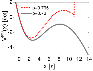
Figure 1: Plot of the trapping potential $V^{(\textsf{at})}(x)$: $p=0.795$ (dashed line) plus a hard wall at $x=11\ell$ [represents the trap at $t=0$] and $p=0.73$ (solid line) [represents the trap at $t>0$]

For the interatomic interaction potential $V^{(\textsf{aa})}(z_{1}-z_{2})$ we choose the Gaussian shape gharashi ; ishmukh2

$$V^{(\textsf{aa})}(x_{1}-x_{2})=-V_{G}\exp\left\{-\frac{(x_{1}-x_{2})^{2}}{2r_{0}^{2}}\right\},$$ (2.5)

where $V_{G}$ and $r_{0}$ - are the depth and range of the interatomic interaction (2.5). The value $r_{0}=0.1\ell$ ishmukh2 ; gharashi - well represents the short-range interaction, which atoms experience at low energies. To parameterize the interaction (2.5) we use the 1D contact coupling strength $g$ which has a simple relation with a 1D scattering length $a$ as $g=-2\hbar^{2}/(ma)$. To compute $a$ we solve the scattering problem for the relative motion of the two-atom system in the absence of the trapping potential ishmukh ; ishmukh2 .

In order to integrate (2.1) we use the split-operator method, which is based on ideas marchuk and has been developed in the works melezhik ; melezhik2 ; melezhik3 in application to confined ultracold atom-atom collisions in waveguide-like traps:

$$\psi(x_{1},x_{2},t+\Delta t)=\exp\left\{-i\frac{\Delta t}{2\hbar}V^{(\textsf{aa})}(x_{1}-x_{2})\right\}$$

$$\exp\left\{-\frac{i\Delta tH_{1}(x_{1})}{\hbar}\right\}\exp\left\{-\frac{i\Delta tH_{2}(x_{2})}{\hbar}\right\}$$

$$\exp\left\{-i\frac{\Delta t}{2\hbar}V^{(\textsf{aa})}(x_{1}-x_{2})\right\}\psi(x_{1},x_{2},t)$$ (2.6)

The action of the operators $\exp\left\{-i\Delta tH_{j}(x_{j})\right\}$ is approximated by the Crank-Nicolson scheme, which maintains the accuracy order of the split-operator scheme (II) to $\mathcal{O}(\Delta t^{3})$. The partial derivatives in (2.3) are approximated by the sixth-order finite-differences.

At large $x_{1}$ and $x_{2}$ the wave function should has a shape of an outgoing wave. This boundary condition can be modeled by introducing into the original Hamiltonian (2.2) a complex absorbing potential (CAP) $iW(x_{j})$ meyer ; lode , which absorbs the wave-packet at the edges of the simulation grid, of the form:

$$W(x_{j})=w_{c}(|x_{j}|-x_{c})^{2}\theta(|x_{j}|-x_{c}),\qquad j=1,2,$$ (2.7)

where $\theta(x)$ is the Heaviside step function. Final results should not depend on a particular choice of the parameters $w_{c}$ and $x_{c}$. Therefore, there is no unique choice of these parameters, but rather a domain where the final results do not significantly change under the variation of them. We find that $w_{c}=-1\hbar\omega\ell^{-2}$ and $x_{c}=25\ell$ lie in that domain.

III RESULTS

III.1 Initial solution and the energy spectum

The first step to integrate Eq.(2.1) is to obtain its initial solution, i.e. $\psi(x_{1},x_{2},t=0)$. As a reference point, we consider the situation where the two-atom system is initially prepared in a deep trap with $p=0.795$. To compute eigenstates and eigenenergies in such a trap we put a hard wall, as in gharashi , at $x=11\ell$ (Fig.1) and assume that both atoms feel the same magnetic field gradient $\mathcal{C}=1894.18$ G/m. This set of parameters mimics the initial state preparation used in the experiments zuern ; zuern2 . The corresponding stationary Schödinger equation is solved by means of the method from ishmukh3 . The energy spectrum in such a trap is shown in Fig.2. We focus on the excited state branches - upper and lower ones. These branches correspond to doubly excited states with respect to relative and center-of-mass motions ishmukh . The nodal patterns of the wave functions is shown in Fig.3. At negative coupling ($g=-1$ in Fig.3) one clearly identifies the two nodes with respect to relative (upper branch) and center-of-mass (lower branch) motion coordinates. When we cross the point $g=0$, the nodal patterns of these states are mixed and at $g=1$ the doubly excited relative motion state, observed for the upper branch at $g=-1$, turns into the doubly excited center-of-mass motion state. The same situation, only vice versa, occurs for the lower branch: the doubly excited center-of-mass state turns into the doubly excited relative motion state. The origin of such nodal pattern mixing is due to rotational symmetry breaking at $g=0$: the anharmonic terms of the trap potential (2.4) lift the doubly degenerate harmonic energy level ishmukh . Similar effect has been observed in sala ; ishmukh ; noid .

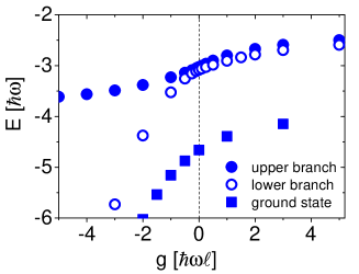
Figure 2: Energy spectrum of the ”closed” trapping potential (2.4) as a function of the coupling strength $g$, using $p=0.795$ and putting a hard wall at $x=11\ell$. Upper and lower excited state branches correspond to the doubly excited states with respect to relative and center-of-mass motions ishmukh .

g=-1	g=0	g=1	g=3
Upper branch
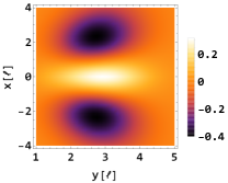
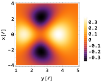
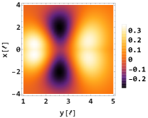
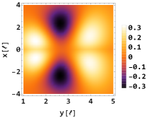
Lower branch

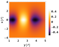
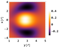
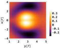
Figure 3: Wave functions of the Hamiltonian (2.2) with $p=0.795$ and a hard wall at $x=11\ell$ at various coupling strength, $g$ (in units of $\hbar\omega\ell$). Here $x=x_{1}-x_{2}$ is the relative motion coordinate and $y=\frac{x_{1}+x_{2}}{2}$ is the center-of-mass motion coordinate.

When computing the time-evolution of the wave function $\psi(x_{1},x_{2},t)$ at $t>0$, using (II), we set $\mathcal{C}_{1}=1886$ G/m and $\mathcal{C}_{2}=1884$ G/m. These values approximately correspond to the values used for the tunneling dynamics used in gharashi which models the actual values used in the experiments zuern ; zuern2 . As was pointed out in gharashi the accurate calculation of the parameters $\mathcal{C}$ should include Breit-Rabi formula. In the present paper we avoid such a consideration and expect that the qualitative picture of the whole tunneling analysis would not be altered significantly.

III.2 Upper branch

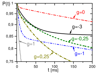
Figure 4: (Color online) Total probability $P(t)$ for various coupling strengths $g$ (in units of $\hbar\omega\ell$) with $p=0.73$.

For an analysis of the tunneling dynamics we consider the total probability $P(t)$

$$P(t)=\iint\limits_{\Omega}dx_{1}dx_{2}|\psi(x_{1},x_{2},t)|^{2},$$ (3.1)

where, for the integration domain $\Omega$, we use the simulation grid $x_{k}\in[-3,40]$. Dependence of a decay rate of the total probability $P(t)$ goes in a non-monotonic manner as a function of the coupling strength $g$. From Fig.4, one can notice that at $g=-0.25\hbar\omega$ the total probability $P(t)$ takes an intermediate value between the total probabilities $P(t)$ at $g=-3\hbar\omega$ and $g=-1\hbar\omega$. When we increase $g$ to $g=0$ the quantity $P(t)$ goes with an even smaller decay rate. Further increasing of $g$, however, leads to approximately monotonic dependence of the decay of $P(t)$ on $g$. This non-monotonic (and monotonic behavior discussed in the next section) behavior is somewhat similar to the behavior observed in ishmukh .

To better understand the origin of such a non-monotonic behavior we pick for the initial wave functions the wave functions at $g=-1\hbar\omega\ell$, $g=0$ and $g=1\hbar\omega\ell$ and compute $P(t)$ for a wide range of the coupling strengths, starting from $g=-3\hbar\omega\ell$ up to $g=1\hbar\omega\ell$ (of course, the computed $P(t)$ differ significantly from $P(t)$, computed with the correct initial state wave functions, i.e. the initial states with the same coupling strengths $g$ as the value of $g$ used for $t>0$). We observe that, for the initial states with $g=0$ and $g=1\hbar\omega\ell$, the non-monotonic behavior still preserves: the decay rate of $P(t)$, starting from $g=-3\hbar\omega\ell$, decreases monotonically with increasing $g$, up to the decay rate of $P(t)$ at $g=0$, and then monotonically increases with increasing $g$. However, with these three different initial states we don’t reproduce the non-monotonic dependence of $P(t)$ between the $g=-3\hbar\omega\ell$ and $g=-1\hbar\omega\ell$, i.e. $P(t)$ at $g=-0.25\hbar\omega\ell$ (Fig.4). This suggests that the origin of such peculiar behavior, perhaps, refers to the initial wave function distribution.

If we divide the whole configuration space into regions (Fig.5) and calculate the partial probabilities

$$P_{k}(t)=\iint\limits_{region~{}k}dx_{1}dx_{2}|\psi(x_{1},x_{2},t)|^{2}$$

$$\hskip 8.5359ptk=0,1,2.$$ (3.2)

at each of the region then it is possible to extract the mean atom number that remains in the trap during the decay of the system. Region $R_{2}$ approximately covers the size of the two-atom trap (we take it as $x_{j}\in[-3,13]$) and therefore $P_{2}$ defines the probability to find the two atoms in the trap, $P_{1}$ defines the probability to find one atom in the trap and $P_{0}$ defines the probability that the two atoms escape from the trap. The mean atom number is defined as

$$\bar{N}(t)=2P_{2}(t)+P_{1}(t).$$ (3.3)

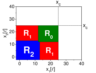
Figure 5: (Color online) Partition of the configuration space into regions $R_{2}$ (the region that covers the trap size), $R_{1}$ and $R_{0}$. $x_{c}$ is the position at which CAP starts.

An analysis of the partial probabilities for the upper branch shows that the tunneling predominately goes into the regions $R_{1}$. Due to the normalization condition, $P_{2}(t)+P_{1}(t)+P_{0}(t)=1$, and that $P_{0}(t)$ is small, we approximate $P_{1}(t)$ as $P_{1}(t)\approx 1-P_{2}(t)$. Hence, the mean atom number is calculated as $\bar{N}(t)\approx P_{2}(t)+1$. The resulting $\bar{N}(t)$ is shown in Fig.6.

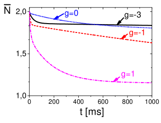
Figure 6: (Color online) Mean particle number $\bar{N}(t)$ for various coupling strength $g$ (in units of $\hbar\omega\ell$).

Since the tunneling goes only into the regions $R_{1}$, within the considered time domain, we can conclude that only the first particle tunnels out of the trap (Fig.6) while the second particle remains in the trap with very small decay rate gharashi .

III.3 Lower branch

The decay rate from the lower branch of the excited states exhibits the monotonic dependence on the coupling strength $g$: the total probability $P(t)$ decays faster with increasing $g$ (Fig.7). From Fig.7 one can observe a non-exponential decay of $P(t)$ at $g=3\hbar\omega\ell$. For high enough values of $g$, the decay from the lower branch goes faster than the decay from the upper branch of the excited states. This can be already noticed when comparing the decay of $P(t)$ at $g=0$ (cf. Fig.4).

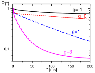
Figure 7: (Color online) Total probability $P(t)$ for various coupling strengths $g$ (in units of $\hbar\omega\ell$) using $p=0.73$ at $t>0$

Another interesting feature of the tunneling from this excited state branch occurs when we explore the transition from the correlated pair tunneling to uncorrelated one by decreasing the barrier, by using lower values of $p$ in (2.4). This transition takes place when the energy level of the excited bound state is close enough to the barrier level and there is strong enough attractive coupling $g$. We observe that the trap value $p=0.68$ (Eq.(2.4)) is sufficient to observe such a transition. We identify the transition by computing the probability current

$$j_{k}(x_{1},x_{2},t)=\frac{\hbar}{2mi}\left(\psi^{\ast}\frac{\partial\psi}{\partial x_{k}}-\psi\frac{\partial\psi^{\ast}}{\partial x_{k}}\right),$$

$$\hskip 5.69046ptk=1,2.$$ (3.4)

From Fig.8, with $p=0.68$, one can notice that $|\textbf{j}(x_{1},x_{2},t)|$ at $g=-2\hbar\omega\ell$ predominantly goes along the $x_{1}=x_{2}$ axis, which represents the tunneling of the two-atom system as a bound object, whereas at higher values of $g$, tunneling goes along the axes $x_{1}$ and $x_{2}$, which indicates a tunneling of the first particle. For higher values of $p$, $p=0.73$, this correlated tunneling channel is significantly suppressed and we observe that the sequential particle tunneling dominates also for the strong attraction, $g=-2\hbar\omega\ell$, and also repulsion. The tunneling rate of the second particle is expected to be negligible for the considered time domain gharashi .

$g=-2\hbar\omega\ell$	$g=0$	$g=3\hbar\omega\ell$
$p=0.68$
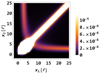
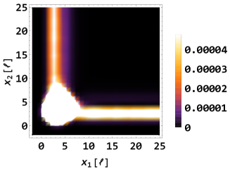
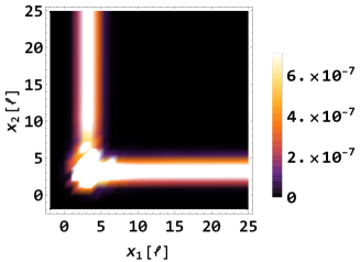
$p=0.73$

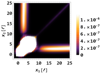
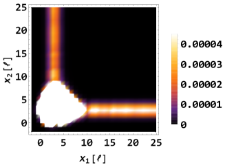
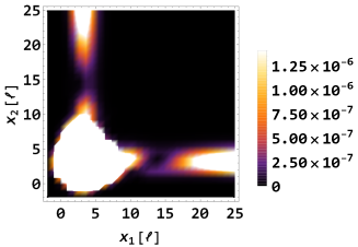
Figure 8: (Color online) Probability current $|\textbf{j}(x_{1},x_{2},t)|$ of the lower excited state branch for the coupling strength values $g/(\hbar\omega\ell)=-2,0,3$ computed at $t=50$ ms. The values of the probability current shown in the legends are in $\omega/\ell$ units (note the different scale for all the graphs).

IV CONCLUSION

We model the two-atom system with a realistic trap potential used in recent experiments zuern ; zuern2 . We have extended the analysis made in gharashi by considering tunneling from other excited states. It has been found that the decay rate from the upper excited state branch goes in a non-monotonic manner as a function of the coupling strength $g$, whereas the tunneling from the lower excited state branch exhibits monotonic dependence as a function of $g$.

We find how a transition from the correlated to uncorrelated tunneling behaves with changing the trap barrier. By decreasing the trap barrier, the correlated pair tunneling manifest itself at strong enough attractive coupling strength $g$. With increasing $g$ the two particles decay in a sequential manner. This transition is found to be absent for higher trap barrier. The particles from the upper branch, for the considered wide range of $g$, decay in the sequential way.

The analysis made in the paper can be extended to problems with more spatial degrees of freedom which can include transverse optical confinement gharashi . It is also interesting to add more particles into the consideration.

References

- (1) A. B. Migdal, Zh. Eksp. Teor. Fiz. Pisma 37, 249 (1959) [Sov. Phys. JETP 10, 176 (1960)].
- (2) T. Maruyama, T. Oishi, K. Hagino, and H. Sagawa, Time-dependent approach to many-particle tunneling in one dimension, Phys. Rev. C 86, 044301 (2012)
- (3) G. Scamps and K. Hagino, Multidimensional fission model with a complex absorbing potential, Phys. Rev. C 91, 044606 (2015).
- (4) P. G. de Gennes, Superconductivity of Metals and Alloys (Westview Press, Boulder, CO, 1999).
- (5) A. J. Leggett, Quantum Liquids, 1st ed. (Oxford University Press, New York, 2006).
- (6) F. Serwane, G. Zürn, T. Lompe, T.B. Ottenstein, A.N. Wenz, and S. Jochim, Deterministic preparation of a tunable few-fermion system, Science 332, 336 (2011).
- (7) G. Zürn, F. Serwane, T. Lompe, A. N. Wenz, M. G. Ries, J. E. Bohn, and S. Jochim, Fermionization of two distinguishable fermions, Phys. Rev. Lett., 108, 075303, (2012).
- (8) G.Zürn, A.N.Wenz, S.Murmann, A.Bergschneider, T.Lompe, and S. Jochim, Pairing in few-fermion systems with attractive interactions, Phys. Rev. Lett., 111, 175302, (2013).
- (9) Z. Idziaszek and T. Calarco, Analytical solutions for the dynamics of two trapped interacting ultracold atoms, Phys. Rev. A 74, 022712 (2006)
- (10) C. Chin, R. Grimm, P. Julienne, and E. Tiesinga, Feshbach resonances in ultracold gases, Rev. Mod. Phys. 82, 1225 (2010).
- (11) M. Rontani, Tunneling theory of two interacting atoms in a trap, Phys. Rev. A 108, 115302 (2012).
- (12) M. Rontani, Pair tunneling of two atoms out of a trap, Phys. Rev. A 88, 043633 (2013).
- (13) S.E. Gharashi and D. Blume, Tunneling dynamics of two interacting one-dimensional particles, Phys. Rev. A 92, 033629 (2015).
- (14) V.S. Melezhik, J.I. Kim and P. Schmelcher, Wave packet dynamical analysis of ultracold scattering in cylindrical waveguides, Phys. Rev. A 76, 053611 (2007).
- (15) V.S. Melezhik, Atoms and Molecules in Strong External Fields (Plenum, New-York and London, 1998) pp.89-94.
- (16) V.S. Melezhik, Mathematical modeling of ultracold few-body processes in atomic traps, EPJ Web Conf. 108, 01008 (2016).
- (17) V. O. Nesterenko, A. N. Novikov, and E. Suraud, Transport of the repulsive bose-einstein condensate in a double-well trap: Interaction impact and relation to the josephson effect, Laser Phys. 24, 125501 (2014).
- (18) P. M. Krassovitskiy and F. M. Pen kov, Contribution of resonance tunneling of molecule to physical observables, J. Phys. B: At. Mol. Opt. Phys. 47, 225210 (2014).
- (19) A. U. J. Lode, A. I. Streltsov, O. E. Alon, H.-D. Meyer, and L. S. Cederbaum, Exact decay and tunnelling dynamics of interacting few-boson systems, J. Phys. B 42, 044018 (2009).
- (20) S. Hunn, K. Zimmermann, M. Hiller, and A. Buchleitner, Tunneling decay of two interacting bosons in an asymmetric double-well potential: A spectral approach, Phys. Rev. A 87, 043626 (2013).
- (21) J. Dobrzyniecki and T. Sowiński, Dynamics of a few interacting bosons escaping from an open well, arXiv:1804.04932v1
- (22) I.S. Ishmukhamedov and V.S. Melezhik, Tunneling of two bosonic atoms from a one-dimensional anharmonic trap, Phys. Rev. A 95, 062701 (2017).
- (23) I.S. Ishmukhamedov, D.S. Valiolda, and S.A. Zhaugasheva, Description of ultracold atoms in a one-dimensional geometry of a harmonic trap with a realistic interaction, Phys. Part. Nuclei Lett. 11: 238 (2014).
- (24) G.I. Marchuk, Methods of Numerical Mathematics, (Springer-Verlag, New York,1975) Sec. 4.3.3
- (25) U. V. Riss and H.-D. Meyer, Calculation of resonance energies and widths using the complex absorbing potential method, J. Phys. B 26, 4503 (1993).
- (26) I.S. Ishmukhamedov, D.T. Aznabayev, and S.A. Zhaugasheva, Two-body atomic system in a one-dimensional anharmonic trap: The energy spectrum, Phys. Part. Nuclei Lett. 12: 680 (2015).
- (27) S. Sala and A. Saenz, Theory of inelastic confinement-induced resonances due to the coupling of center-of-mass and relative motion, Phys. Rev. A 94, 022713 (2016).
- (28) D. W. Noid, M. L. Koszykowski, and R. A. Marcus, Comparison of quantal, classical, and semiclassical behavior at an isolated avoided crossing, J. Chem. Phys. 78, 4018 (1983).