Multi-Task Handwritten Document Layout Analysis

Abstract

Document Layout Analysis is a fundamental step in Handwritten Text Processing systems, from the extraction of the text lines to the type of zone it belongs to. We present a system based on artificial neural networks which is able to determine not only the baselines of text lines present in the document, but also performs geometric and logic layout analysis of the document. Experiments in three different datasets demonstrate the potential of the method and show competitive results with respect to state-of-the-art methods.

Keywords— document layout analysis, text line detection, baseline detection, semantic segmentation, zone segmentation, handwritten text recognition

1 Introduction

Handwritten Text Processing (HTP) systems such as Handwritten Text Recognition (HTR) [1], Keyword Spotting (KWS) [2] and Information Retrieval from Handwritten Documents [3] are well-known problems where an image of a handwritten document is used as an input and some kind of text-related information is expected as output. But for all current HTP systems, the image is expected to contain just a single short handwritten sequence; that is, only one line of handwritten text is processed at once. However, since the main goal of those systems is to process not just a single line, but a complete paragraph or even a complete document, a previous system is needed in order to extract the required lines from the whole page and, in an upper level, to segment the different zones of the page (paragraph, marginal notes, illustrations, page number, etc.) in a meaningful manner (normally consistent with the reading order).

Consequently, both test line extraction and image segmentation into relevant zones constitute a very important stage of any HTP system, generally related as Document Layout Analysis (DLA). Commonly this process is divided into two sub problems [4]. First, geometric layout analysis aims at producing a description of the geometric structure of the document ( i.e. where each zone is placed, its shape and relationship with other zones). This structure allows us to describe the document layout at different levels of detail (e.g. a set of text lines can be viewed at higher level as a paragraph). Second, the classification of those zones into their logical role (title, paragraph, illustration, etc.) is called the logical layout analysis. Although, logical layout analysis is not necessary for zone segmentation nor for text line extraction, it is a very important step required to present the results of HTP systems in the same context as the input document (e.g. the transcript of some text line can be presented as a title or other type only if the zone label is defined, otherwise we can just provide the plain transcript).

In most recent formulations the determination of text lines focus on the detection of their baselines (the imaginary lines upon which the lines of text rest) rather than a detailed polygons surrounding the text lines. Owing to the fact that a baseline is defined by only a few points, humans can easily label on the text lines of an image, without having to deal with the cumbersome detailed segmentation of each text line region.

Once some DLA system provides a baseline for each text line in a document it can be easily reviewed and corrected by the user. Also, rough segmentation of a text line can be straightforwardly obtained from its baseline, and because state-of-the-art HTP systems are able to filter out a lot of noise present in the input, this roughly segmented lines can be used by the HTP system with almost no negative impact on performance [5].

It is very important to notice the huge impact the context provided by the logical layout analysis can have in the performance of HTP systems. For example a well segmented text line labeled as a part of the page number text zone is expected to have only digits; then the search space for the HTP system can be reduced drastically.

In this work, we present a system based on Artificial Neural Networks, which is able to detect the baselines, layout zones, and labels of that zones, from the digital image of the document. It is an integrated approach where baselines and text zones are detected and segmented in a single process, and the relationship between them is defined in a top-down way.

The rest of this paper is organized as follows. In Sec. 2 related work is discussed. Then, the proposed method is presented in Sec. 3. Afterwards, experimental setup is presented in Sec. 4, while results are reported in Sec. 5. Finally, we draw some conclusions in Sec. 6.

2 Related work

Comprehensive surveys about document image analysis [6, 7, 8] and [9] provide a very good insight about the state-of-the-art algorithms for document segmentation, including DLA.

DLA methods can be divided typologically into three groups by the problem they are developed to solve: text line extraction (included baseline detection), zone segmentation and zone labeling. Most of the methods focus on only one of these groups, or provide a separate algorithm for each one. In contrast, the method we present in this work encompasses all three groups under the same model.

2.1 Text line extraction

This is the group to which most methods belong to, mainly because its direct applicability to HTP systems. The main goal of these methods is to segment the input image into a set of smaller images, each of which contains a single text line.

Methods such as those presented in [10, 11, 12, 13, 14] rely on connected components extraction after some filtering stage, while other methods such as [15, 16] use a tracer function to separate the different text lines after applying a blur to the input image. Other methods rely on Hidden Markov Models [17, 18, 19] or Recurrent Neural Networks [20] to model the vertical sequential structure of the text lines, or Convolutional Neural Networks [21, 22, 23] to classify each pixel of the image between text line and non-text line.

2.2 Zone segmentation

Most of the methods for text line extraction rely on the assumption that input images contain a single region of text; which means, documents with a single column layout, or images previously segmented into the different text zones. Zone segmentation aims at providing this level of page image segmentation.

Several methods are based on some kind of pixel-level classifier (Multilayer Perceptron [24, 25, 26, 14], Conditional Random Fields [27], Definite Clause Grammars [28], Gaussian Mixture Models and Support Vector Machines [26]) whose input is a set of handcrafted features from the input images (Gabor filters, Kalman filters, Connected Components, Multi-scale images, etc). Others aim to provide an interactive framework to review the results of the zone segmentation algorithm [29].

2.3 Zone labeling

Methods of this group are often closely related with methods of the previous one, but some of them focus only on separating text from non-text zones [30, 26, 25, 23] (which can be considered as a simplified form of Zone labeling). Other approaches go further to provide not just the segmentation of the zones but also the corresponding zone labels (three different zones are labeled in [27], two in [24] and six in [28]).

Any of the three groups listed before can be used to help the processing of any other group (e.g. segmented zones can be used to constrain the search space for line detection and vice-versa), which is a causality dilemma in the design of any DLA system. An integrated method, as proposed in this paper, provides a solution to this dilemma where the relevant dependencies are incorporated internally in the model.

3 Proposed Method

An overview of the proposed method for Document Layout Analysis is given in Fig. 1. The method consists of two main stages.

• Stage 1: Pixel level classification, for zones and baselines.

• Stage 2: Zone segmentation and baseline detection.

In the first stage an Artificial Neural Network (ANN) is used to classify the pixels of the input image ($\bm{x}\in\mathbb{R}^{w\times h\times\gamma}$, with height $h$, width $w$ and $\gamma$ channels) into a set of regions of interest (layout zones and baselines). This is a crucial stage in the process, where information from the images is extracted, while next stage is designed to provide that information in a usefull format.

In the second state a contour extraction algorithm is used to consolidate the pixel level classification into a set of simplified zones delimited by closed polygons. Then a similar process is carried on inside each zone to extract the baselines. In this way we obtain the location and label of each zone, and the baselines that they contain.

Figure 1: Proposed method overview. $\bm{x}$ is the input image and $\bm{y}^{*}$ is the best hypothesis from the ANN. Better seeing in color.

3.1 Stage 1: Pixel Level Classification

Layout Analysis can be defined as a Multi-Task problem [31] where two tasks are defined:

• Task-1: Baseline detection.

• Task-2: Zone segmentation and labeling.

Task-1 consists in obtaining the baseline of each text line present in the input image. This baseline is used to extract the sub-image of the text line and feed it into some HTP system. On the other hand, Task-2 consists in assigning those baselines into the different zones they belong to. For example, baselines that are members of the main paragraph should be grouped together into a zone, while the ones that are members of a marginal note should be grouped into another one. Since each line belongs to a different context, that information can be used by the HTP system to provide more accurate hypotheses.

In a general manner we can define a multi-task variable $\bm{y}=[\bm{y}^{1},\dots,\bm{y}^{T}]$, where $\bm{y}^{t}=(y^{t}_{ij}),1\leq i\leq w,1\leq j\leq h,1\leq t\leq T$ and $y^{t}_{ij}\in\mathcal{Y}^{t}=\{1,\dots,K^{t}\}^{w\times h}$ with $K^{t}\in\mathbb{N}_{+}$ being the finite number of classes associated with the $t$-th task. The solution of this problem for some test instance $\bm{x}$ is given as the following optimization problem:

$$\hat{\bm{y}}=\operatorname*{arg\,max}_{\bm{y}}\mathrm{p}(\bm{y}\mid\bm{x})$$ (1)

where the conditional distribution $\mathrm{p}(\bm{y}\mid\bm{x})$ is usually unknown and has to be estimated from training data $D=\{(\bm{x}_{i},\bm{y}_{i})\}^{N}_{n=1}=\{(\bm{X},\bm{Y})\}$.

In our specific two-task case ($T=2$), Task-1 ($t=1$) is a binary classification problem, then $K^{1}=2$ (background, baseline). On the other hand, Task-2 ($t=2$) is a multi-class problem where $K^{2}$ is equal to the number of different types of zones in the specific corpus, plus one for the background; normally, the number of types of zones is small (e.g. $K^{2}<15$).

The Conditional Generative Adversarial Network presented in [32] has shown very good results in several problems versus the non-adversarial neural networks. In this work the conditional distribution $\mathrm{p}(\bm{y}\mid\bm{x})$ is estimated by a modified version of the Conditional Generative Adversarial Network, where the output layer of the generative network is replaced by a softmax layer for each task to ground the network to the underlying discriminative problem (this can be considered as a type of Discriminative Adversarial Network, as presented in [33]). The ANN is trained using labeled data as depicted in Fig. 2, where the color represents the class label of each task.

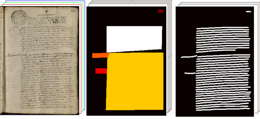
Figure 2: Visualization of the encoded ground-truth to feed the ANN during training. From left to right: Original image ($\bm{x}$), Task-2 pixel-level ground-truth ($\bm{y}^{t=2}$), Task-A pixel-level ground-truth ($\bm{y^{t=1}}$). The colors in the ground-truth images represents the class label of each task. Better seeing in color.

3.1.1 ANN Inference

An ANN, called M-net, is trained, as discussed in Sec. 3.1.2, to estimate the posterior probability in Eq. (1), as depicted in Fig. (3) where $\mathcal{M}(\cdot)$ is the output of the latest layer of M-net, and the $\operatorname*{arg\,max}$ operation is computed element-wise and separately for each task involved, this is:

• Task-1:

  $$y^{*1}_{i,j}=\operatorname*{arg\,max}_{y\in\mathcal{Y}^{1}=\{0,1\}}\mathcal{M}_{i,j,y}(\bm{x}),\quad 0\leq i\leq w,0\leq j\leq h$$ (2)

• Task-2:

  $$y^{*2}_{i,j}=\operatorname*{arg\,max}_{y\in\mathcal{Y}^{2}=\{1,\dots,K^{2}\}}\mathcal{M}_{i,j,y}(\bm{x}),\quad 0\leq i\leq w,0\leq j\leq h$$ (3)

Notice this optimization problem rather corresponds to a simplified model, where no restrictions are formulated based on the prior knowledge we have of the problem (e.g. a page number zone is not expected to be between paragraphs). Although some prior knowledge is learned by the ANN during training, the experience in other areas such as HTR and KWS has demonstrated very positive results when priors are explicitly considered[2]. Consequently, in a future version of the proposed method a set of structural restrictions, modeled as a prior-probability of $\bm{y}$, will be added to take into account that valuable knowledge.

Figure 3: Inference set-up for ANN.

3.1.2 ANN Objective and Training

Training an ANN is very dependent on the selected objective function, since it defines what we want to learn. Classical objective functions are defined directly by how we want to approximate the probabilistic distribution of the data (mean square error, cross entropy, etc), while new adversarial networks are using a composed objective function to improve performance.

The objective function we want to minimize is composed of the interaction between two separated ANNs, that we call A-net and M-net, see Fig. 4. The A-net is trained to distinguish between real labels (from $D$) and produced labels (sometimes called fake labels) from M-net (notice A-net is used only to help train M-net, and is discarded at inference time).

Figure 4: Training set-up for ANN.

In the A-net network the cost function is the classical cross-entropy loss, where only two classes are defined, “1” when the input of the network belongs to the real labels, and “0” when the labels are generated by M-net, that is:

$$\mathcal{L}_{A}(\bm{X},\bm{Y})=\frac{1}{2}\left\{\mathcal{L}_{A}^{1}(\bm{X},\bm{Y})+\mathcal{L}_{A}^{0}(\bm{X},\bm{Y})\right\},\quad(\bm{X},\bm{Y})\in D$$ (4)

according to

$$\mathcal{L}_{A}^{1}(\bm{X},\bm{Y})=\frac{-1}{N}\sum^{N}_{n=1}\log\mathcal{A}(\bm{x}_{n},\bm{y}_{n})$$ (5)

and

$$\mathcal{L}_{A}^{0}(\bm{X},\bm{Y})=\frac{-1}{N}\sum^{N}_{n=1}\log(1-\mathcal{A}(\bm{x}_{n},\operatorname*{arg\,max}_{\bm{y}}\mathcal{M}(\bm{x}_{n})))$$ (6)

where $\mathcal{A}(\cdot)$ is the output of the A-net and $\mathcal{M}(\cdot)$ is the output of the M-net.

Hence $\mathcal{L}_{A}(\bm{X},\bm{Y})$ simplifies to

$$\mathcal{L}_{A}({\bm{X},\bm{Y}})=\frac{-1}{2N}\sum^{N}_{n=1}\log\mathcal{A}(\bm{x}_{n},\bm{y}_{n})+\;\log(1-f_{A}(\bm{x}_{n},\operatorname*{arg\,max}_{\bm{y}}\mathcal{M}(\bm{x}_{n})))$$ (7)

On the other hand, the main network M-net performs the actual set of tasks we aim at. In the M-net the cost function is composed by the contribution of two cost functions, whose balance is controlled by the hyperparameter $\lambda$

$$\mathcal{L}_{M}(\bm{X},\bm{Y})=\frac{-1}{N}\sum^{N}_{n=1}\mathcal{L}(\bm{x}_{n},\bm{y}_{n})+\lambda\mathcal{L}_{A}^{0}(\bm{x}_{n},\bm{y}_{n})$$ (8)

where $\mathcal{L}^{0}_{A}(\cdot)$ (Eq. 6) drives the network to fool the network A, and $\mathcal{L}(\bm{x}_{i},\bm{y}_{i})$ is the cross-entropy loss, which drives the network to learn the probability distribution of the training data:

$$\mathcal{L}(\bm{x},\bm{y})=\frac{-1}{Twh}\sum^{T}_{t=1}\sum^{w}_{i=1}\sum^{h}_{j=1}\sum^{K^{t}}_{c=1}\bm{y}^{t}_{i,j,c}\log(\mathcal{M}^{t}_{i,j,c}(\bm{x}))$$ (9)

where $T$ is the number of tasks to be performed, $K^{t}$ is the number of classes of the task $t,1\leq t\leq T$, the binary target variable $\bm{y}^{t}_{i,j,c}\in\{0,1\}$ has a 1-of-$K^{t}$ coding scheme indicating the correct class, and $\mathcal{M}^{t}_{i,j,c}(x)$ is the output of the M-net network for the Task-$t$ and class $c$, interpreted as $\mathcal{M}^{t}_{i,j,c}(\bm{x})=\mathrm{p}(\bm{y}^{t}_{i,j,c}~{}=~{}1|\bm{x}_{i,j})$ (i.e. the posterior probability of the pixel $i,j$ of the input image belongs to the class $c$ for task $t$).

Both ANNs are optimized in parallel, following the standard approach from [34]: we alternate between one gradient descent step on M-net, and one step on A-net, and so on.

The training set-up is depicted in Fig. 4, where the “Mux” block is a standard multiplexer between the “real” label ($\bm{y}_{n}$) and the “fake” one from the M-net.

3.2 Stage 2: Zones Segmentation and baseline detection

On this stage information extracted from the images in previous stage is shaped in a useful way, into a set piece-wise linear curves and polygons.

3.2.1 Contour Extraction

Let a test instance $\bm{x}$ and its pixel level classification $\bm{y}^{*}$ obtained in the previous stage be given. First, the contour extraction algorithm presented by Suzuky et al. [35] is used for each zone over $\bm{y}^{2}$ to determine the vertices of its contour. This algorithm provides a set of contours $\Phi_{k}=\{\phi_{1},\phi_{2},...,\phi_{R}\},k\in\mathcal{Y}^{2},R\geq 0$. Then, for each contour in $\Phi_{k}$ the same extraction algorithm is used over $\bm{y}^{1}$ to find the contours where baselines are expected to be, but restricted to the area defined by the contour $\phi_{r},1\geq r\geq R$. In this step, a new set of contours $L_{k,r}={l_{1},l_{2},\dots,l_{S}};S\geq 0$ are found.

Finally, each contour $l_{s},\,0\!\geq\!s\!\geq\!S$ is supposed to contain a single line of text, whereby a simple baseline detection algorithm is applied to the section of the input image within the contour $l_{s}$ (see Sec. 3.2.2).

Notice that Task-1 and Task-2 can be treated independently using the same formulation above by simply ignoring the network output associated to the task we are not interested in. Then, in Stage 2 we set the regions of interest to be only one with size equal to the input image, as defined in Eq. (10), to perform Task-1 only.

$$\Phi_{k}=\Phi_{1}=\{\phi_{1}\};\phi_{1}=[(0,0),(w,0),(w,h),(0,h)]$$ (10)

Similarly to perform Task-2 alone, we just return $\Phi_{k},\forall k\in\mathcal{Y}^{2}$, without further search inside those contours.

3.2.2 Baseline detection algorithm

Once a text line contour $l_{s}$ is detected, a very simple algorithm can be used to detect the baseline associated to that specific text line (under the assumption that there is only one text line per contour). Each baseline is first straightfordwardly represented as a digital curve.

The pseudo code of the algorithm is presented on Alg. 1. First the input image $\bm{x}$ is cropped with the polygon defined in $l_{s}$, and it is binarized using Otsui’s algorithm. Then, we define the lowest black pixel of each column in the binarized image as a point of the digital curve we are searching for. Finally, as a result of Alg. 1 line 7, the number of points of the digital curve $\rho$ is equal to the number of columns of the cropped image $Y$. In order to reduce the number of points of $\rho$ and remove some outliers, the algorithm presented by Perez et al. [36] to find an optimal piece-wise linear curve with only $m$ vertices is used.

Data: an image $\bm{x}$, a contour $l_{s}$, number of vertex of output piece-wise linear curve $m$

Result: piece-wise linear curve $v$

1 $I=crop(\bm{x},l_{s})$

2$Y=Otsu(I)$

3$\rho=[]$

4for i in rows($Y$) do

5       for j in columns($Y$) do

6             if $Y_{i,j}==1$ then

7                   $\rho[j]=(j,i)$

8             end if

9            

10       end for

11      

12 end for

$v$ = reducePoly($\rho$,$m$)

Algorithm 1 Baseline detection algorithm

4 Experimental Set-up

To assess the performance of the proposed method we test it on three publicly available datasets: cBAD, Bozen, and a new dataset called Oficio de Hipotecas de Girona (OHG).

OHG is a new dataset introduced in [37] for HTR and here for DLA. The ground-truth is annotated both with baselines and zones (segmentation and several labels) (details on 4.4.1), which will allows us to carry out more detailed experiments with complex layout images.

All experiments are conducted using the same hardware, a single NVIDIA TitanX GPU installed along with an Intel Core i5-2500K@3.30GHz CPU with 16GB RAM. The source code, along with the configuration files to replicate these experiments, are available at https://github.com/lquirosd/P2PaLA.

4.1 Ground-truth

Ground-truth is recorded in PAGE-XML format because it allows us to manually annotate and review the elements (baselines and zones) easily, as they can be defined by piece-wise linear curve or polygons of just few vertices.

The ground-truth is then processed to encode the data into the 1-of-$K^{t}$ coding scheme in order to train the ANNs ( Eq. 9). An example of this ground-truth is shown in Fig. 2, where each color represents a different value in the encoding.

4.2 Artificial Neural Network Architecture

As mentioned in Sec. 3.1, the proposed ANN architecture is very similar to the one presented by [32], but it was modified to perform a discriminative rather than a generative processing. The main hyper-parameters of each part of the ANN are reported below, following the convention presented in [32], where Ck denotes a Convolution-BatchNorm-LeakyReLU layer with k filters, and CDk denotes a Convolution-BatchNorm-Dropout-ReLU layer with a dropout rate of 0.5.

4.2.1 A-net Network Architecture

This network is a simple single output Convolutional Neural Network, trained as explained in Sec. 3.1.2. Its main parameters are:

• number of input channels: defined by the number of channels of the input image (3 for RGB images) plus one more for each task involved. In the case of two tasks and RGB images number of input channels is 5.

• Architecture: C64-C128-C256-C512-C512-C512-Sigmoid.

• Convolution filters: $4\times 4$, stride 2.

4.2.2 M-net Network Architecture

This network is structured as an encoder-decoder architecture called U-Net [38]. U-Net differs from a common encoder-decoder due its skip connections between each layer $i$ in the encoder and layer $n-i$ in the decoder, where $n$ is the total number of layers. Main parameters are:

• number of input channels: defined by the number of channels of the input image (3 for RGB images).

• Architecture:

  • encoder: C64-C128-C256-C512-C512-C512-C512-C512

  • decoder: CD512-CD1024-CD1024-C1024-C1024-C512-C256-C128-SoftMax, where LeakyReLU layers are changed to ReLU.

  • Convolution filters: $4\times 4$, stride 2.

4.2.3 Training and Inference

To optimize the networks we follow [32], using minibatch SGD and Adam solver [39], with a learning rate of 0.0001, and momentum parameters $\beta_{1}=0.5$ and $\beta_{2}=0.999$. Also, we use weighted loss from [40], to overcome the imbalance problem in Task-2. The weight is computed as $w_{k}=\frac{1}{\log(c+p_{k})},k\in\mathcal{Y}^{t},c\geq 0$, where $p_{k}$ is the prior-probability of the $k$-th value associated with the task.

Affine transformations (translation, rotation, shear, scale) and Elastic Deformations [41] are applied to the input images as a data augmentation technique, where its parameters are selected randomly from a restricted set of allowed values, and applied on each epoch and image with a probability of 0.5.

In our experiments, we use the maximum batch size allowed by the hardware we have available: 8 images of size $1024\times 768$ on a single Titan X GPU.

4.3 Evaluation Measures

4.3.1 Baseline Detection

We report precision (P), recall (R) and its harmonic mean (F1) measures as defined specifically for this kind of problem in [42]. Tolerance parameters are set to default values in all experiments (see [42] for details about measure definition, tolerance values and implementation details).

4.3.2 Zone Segmentation

We report metrics from semantic segmentation and scene parsing evaluations as presented in [43]:

• Pixel accuracy (pixel acc.): ${\sum_{i}\eta_{ii}}/{\sum_{i}\tau_{i}}$

• Mean accuracy (mean acc.): $1/K^{t=2}\sum_{i}\eta_{ii}/\tau_{i}$

• Mean Jaccard Index (mean IU): $(1/K^{t=2})\sum_{i}\eta_{ii}/(\tau_{i}+\sum_{j}\eta_{ji}-\eta_{ii})$

• Frequency weighted Jaccard Index (f.w. IU): $(\sum_{\kappa}\tau_{\kappa})^{-1}\sum_{i}\tau_{i}\eta_{ii}/(\tau_{i}+\sum_{j}\eta_{ji}-\eta_{ii})$

where $\eta_{ij}$ is the number of pixels of class $i$ predicted to belong to class $j$, $K^{t=2}$ is the number of different classes for the task $t=2$, $\tau_{i}$ the number of pixels of class $i$, and $\kappa\in\mathcal{Y}^{t=2}$.

4.4 Data Sets

4.4.1 Oficio de Hipotecas de Girona

The manuscript Oficio de Hipotecas de Girona (OHG) is provided by the Centre de Recerca d’Història Rural from the Universitat de Girona (CRHR). This collection is composed of hundreds of thousands of notarial deeds from the XVIII-XIX century (1768-1862) [44]. Sales, redemption of censuses, inheritance and matrimonial chapters are among the most common documentary typologies in the collection. This collection is divided in batches of 50 pages each, digitized at 300ppi in 24 bit RGB color, available as TIF images along with their respective ground-truth layout in PAGE XML format, compiled by the HTR group of the PRHLT center and CRHR. OHG pages exibit a relatively complex layout, composed of six relevant zone types; namely: $pag, $tip, $par, $pac, $not, $nop, as described in Table 1. An example is depicted in Fig. 5.

Table 1: Layout regions in the OHG dataset.

ID	Description
$pag	page number.
$tip	notarial typology.
$par	a paragraph of text that begins next to a notarial typology.
$pac	a paragraph that begins on a previous page.
$not	a marginal note.
$nop	a marginal note added a posteriori to the document.

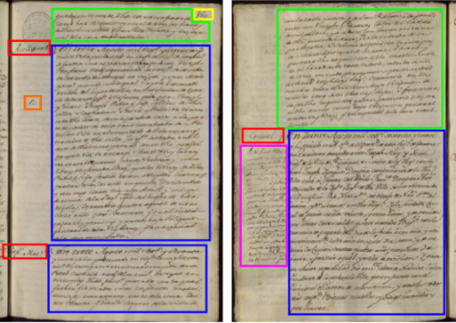
Figure 5: Examples of pages with different layouts, belonging to the Oficio de Hipotecas de Girona dataset. Yellow: $pag, red: $tip, green: $pac, blue: $par, fuchsia: $not, orange:$nop (better seeing in color).

In this work we use a portion of 350 pages from the collection, from batch b004 to batch b010, divided ramdomly into training and test sets, 300 pages and 50 pages respectively. Main characteristics of this dataset are summarized on Table 2.

Table 2: Main characteristics of the OHG dataset.

Batch	#Lines	#Zones
		$par	$pac	$tip	$pag	$nop	$not
b004	1960	72	35	67	24	28	6
b005	1985	73	41	71	25	31	2
b006	1978	68	42	68	25	24	4
b007	1762	60	33	62	19	26	1
b008	1963	69	39	69	24	30	3
b009	1976	75	40	75	25	34	2
b010	2023	71	38	71	25	43	3
Total	13647	488	268	483	167	216	21

4.4.2 cBAD dataset

This dataset was presented in [45] for the ICDAR 2017 Competition on Baseline Detection in Archival Documents (cBAD). It is composed of 2035 annotated document page images that are collected from 9 different archives. Two competition tracks an their corresponding partitions are defined on this corpus to test different characteristics of the submitted methods. Track A [Simple Documents] is published with annotated text regions and therefore aims to evaluate the quality of text line segmentation (216 pages for training and 539 for test). The more challenging Track B [Complex Documents] provides only the page area (270 pages for training and 1010 for test). Hence, baseline detection algorithms need to correctly locate text lines in the presence of marginalia, tables, and noise. The dataset comprises images with additional PAGE XMLs, which contain text regions and baseline annotations.

4.4.3 Bozen dataset

This dataset consists of a subset of documents from the Ratsprotokolle collection composed of minutes of the council meetings held from 1470 to 1805 (about 30.000 pages)[46]. The dataset text is written in Early Modern German by an unknown number of writers. The public dataset is composed of 400 pages (350 for training and 50 for validation); most of the pages consist of a two or three zones with many difficulties for line detection and extraction.

5 Results

5.1 Oficio de Hipotecas de Girona

The dataset is divided randomly into a training and a test set, 300 pages and 50 pages respectively. Experiments are conducted on incremental training subsets from 16 to 300 training images, for Task-1 and Task-2.

Two experiments are performed using this dataset. First, the system is configured to perform only Task-1 giving as a result only the baselines detected in the input images. Second, the system is configured to perform both tasks in a integrated way, giving as a result both the baselines and the layout zones (both segmentation and labels).

Baseline detection precision and recall results for both experiments are reported in Table 3 and F1-measure is depicted in Fig. 6. Even though there are statistically significant differences between the results of performing Task-1 alone and performing both tasks, the slight degradation when both tasks are solved simultaneously is admissible because of the benefit of having not only the baselines detected, but also the zones segmented and labeled. Moreover, when we have enough training images the F1 difference becomes small. Also, there is no appreciable impact in the training time required by the system when we use two tasks or only one (see Fig. 7).

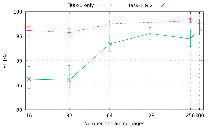
Figure 6: F1 measure for OHG using different number of training pages. Task-1 defined as baseline detection only, and Task-1 & 2 as baseline detection plus zone segmentation and labeling.

Table 3: Precision (P) and Recall (R) results for Task-1 of OHG, when system is trained for Task-1 only and when is trained for both tasks, using different number of training pages. Nonparametric Bootstrapping confidence intervals at 95%, 10000 repetitions are provided.

# of pages	Both tasks		Task-1 only
	P	R	P	R
16	81.5 [78.6,84.1]	92.6 [90.9,94.1]	93.3 [95.1,97.3]	96.0 [95.2,96.7]
32	79.6 [76.1,83.1]	95.1 [94.3,95.8]	96.2 [95.3,97.1]	95.3 [94.2,96.2]
64	91.8 [89.1,94.3]	95.9 [95.1,96.6]	97.5 [96.9,98.1]	97.5 [96.9,97.9]
128	94.8 [93.1,96.4]	96.5 [95.7,97.1]	98.0 [97.5,98.4]	97.6 [97.1,98.1]
256	93.3 [90.2,95.9]	96.4 [95.7,97.1]	98.2 [97.8,98.6]	98.0 [97.5,98.6]
300	96.2 [94.1,97.9]	97.1 [96.4,97.7]	98.4 [98.1,98.7]	97.7 [97.2,98.1]

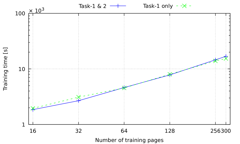
Figure 7: Training time required on OHG experiments. The trend is linear with respect to the number of pages. Better seeing in color.

The recall measure obtained in both experiments is very stable across the number of training images, while precision is closely related to the quality of the zones segmented in the Task-2, see Fig. 8 and 9.

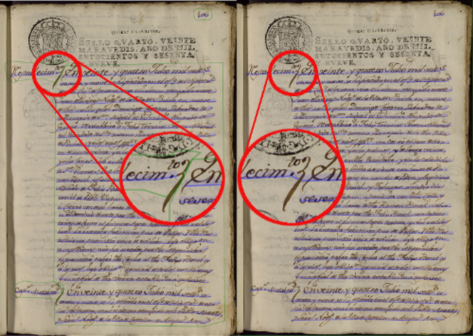
Figure 8: Example of OHG results. In the left zone segmentation prevents the baselines to be merged (Task-1 and Task-2 are performed in an integrated manner). In the right the baselines are merged (Task-1 is performed alone). Better seeing in color.

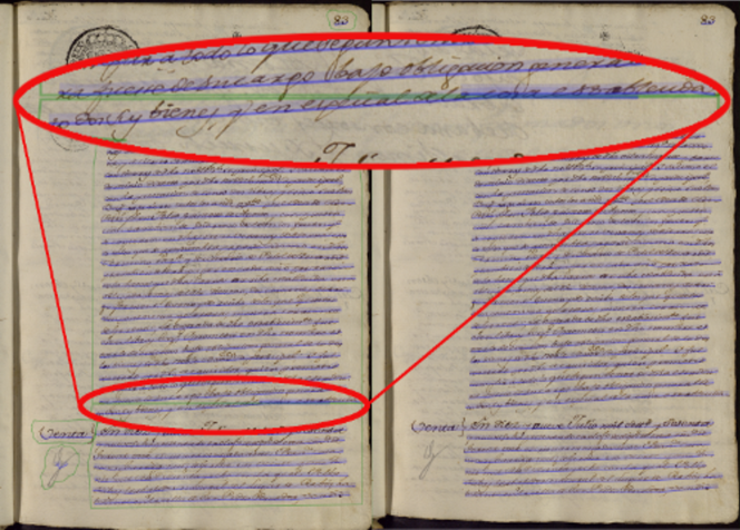
Figure 9: Example of OHG results, where zone segmentation forces baseline to split. Left side is an example where Task-1 and Task-2 are performed, right side is an example when only Task-1 is performed. As remarked, a baseline is divided into two at the point where intersects the zone boundary. Better seeing in color.

Zone segmentation results are reported on Fig. 10. As expected, an improvement with increasing number of training images is observed until 128 images. There the results keep varying but without significant statistical difference.

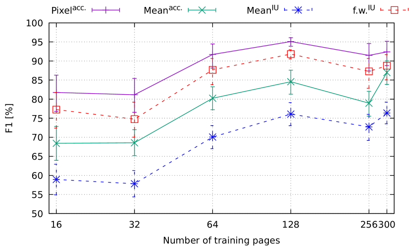
Figure 10: Results for Task-2 of OHG. Nonparametric Bootstrapping confidence intervals at 95%, 10000 repetitions. Better seeing in color.

5.2 cBAD

For this work, only Track B documents are used to train the system. The ground-truth of the test set is not available to the authors, whereby metrics are computed through the competition website.

The system was trained through 200 epochs to perform Task-1 only, because no ground-truth is available for Text Zones in the dataset. Training time was around 3.75 hours using 270 training images on a mini-batch of 8.

Results are reported in Table 4, along with state-of-the-art results presented in the competition and two others recently published (dhSegment, ARU-Net). The proposed approach achieved very competitive results on such a heterogeneous dataset, without significant statistical difference with respect to the winner method of the competition (DMRZ). But below ARU-Net latest result, which we believe is mainly due to the simple baseline detection algorithm we used in Stage 2.

Table 4: Precision (P) and Recall (R) results for the cBAD test set (Task-1 only). Nonparametric Bootstrapping confidence intervals at 95%, 10000 repetitions.

Method	P	R	F1
IRISA	69.2	77.2	73.0
UPVLC	83.3	60.6	70.2
BYU	77.3	82.0	79.9
proposed	84.8 [83.9, 85.7]	85.4 [84.4, 86.4]	85.1
DMRZ	85.4	86.3	85.9
dhSegment [23]	82.6	92.4	87.2
ARU-Net [22]	92.6	91.8	92.2

Main errors are related to merged baselines or missing lines in very crowded areas. An example of those errors is shown in Fig. 11.

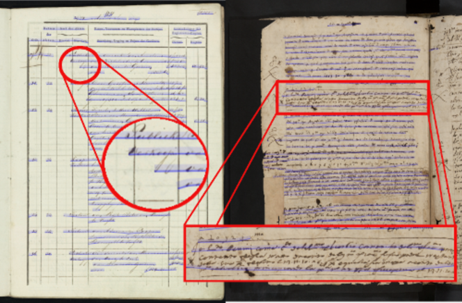
Figure 11: Example of errors in cBAD results produced by the proposed approach. Merged baselines are shown in the left, where adjacent lines in a table are detected as a single one. Missing baselines are showed in the right. Better seeing in color.

5.3 Bozen

Experiments on this work are conducted using the training/validation splits defined by the authors of the dataset, as training and test respectively.

The system was trained through 200 epochs to perform tree different experiments: (I) only Task-1, (II) integrated Task-1 and Task-2 and (III) only Task-2. Training time for each experiment was around 4.75 hours using 350 training images and a mini-batch of 8.

A F1 measure of 97.4% has been achieved on experiment (I), while results achieved on experiment (II) have no significant statistical difference (as shown in Table 5) but with the benefit of obtaining the zones.

Results of experiment (I) can be compared with [22] where a 97.1% F1 measure is reported, which have no significant statistical difference with the results reported here.

Table 5: Precision (P), Recall (R), F1, Pixel accuracy (Pixel^acc.), Mean Pixel accuracy (Mean^acc.), Mean Jaccard Index (Mean^IU) and Frequency weighted Jacard Index (f.w.^IU) results for the Bozen test set. Nonparametric Bootstrapping confidence intervals at 95%, 10000 repetitions.

Metric	Task-1 only	Task-1 and 2	Task-2 only
Baseline Detection
P [%]	95.8 [92.7, 97.8]	94.5 [92.9, 95.9]	–
R [%]	99.1 [98.6, 99.4]	98.9 [98.5, 99.3]	–
F1 [%]	97.4	96.6	–
Zone Segmentation
Pixelacc. [%]	–	95.5 [94.8, 96.1]	95.3 [94.6, 96.0]
Meanacc. [%]	–	91.4 [90.1, 92.7]	93.3 [92.1, 94.5]
MeanIU [%]	–	84.5 [83.1, 85.8]	82.7 [81.3, 84.1]
f.w.IU [%]	–	91.6 [90.5, 92.6]	91.3 [90.2, 92.4]

An example of the errors obtained in this experiments is shown in Fig. 12, where those differences do not generally affect the results of subsequent HTP systems.

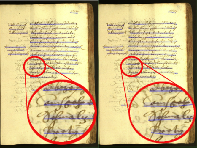
Figure 12: Example of Bozen result. Left image is the ground-truth and at the right is the output of the system. Most of the differences are found at the beginning or the end of the baseline. Better seeing in color.

Zone segmentation and labeling results of experiments (II) and (III) indicate that there is no significant loss in the quality of the results obtained when the system is trained to perform only one of the tasks or both integrated. On the other hand, the average computation time per page at test is reduced by 68% (1.13 s and 0.36 s respectively) as expected.

6 Conclusions

In this paper we present a new multi-task method for handwritten document layout analysis, which is able to perform zone segmentation and labeling, along with baseline detection, in a integrated way, using a single model. The method is based on discriminative ANN and a simple contour and baseline detection algorithms.

We conducted experiments in three different datasets, with promising results on all of them without model reconfiguration or hyper-parameter tuning.

The integrated model tasks) the ANN parameters across tasks without significant degradation in the quality of the results.

Baseline detection results in OHG and Bozen are good enough for most HTR and KWS applications, while cBAD results may not be enough for HTR applications if high quality transcripts are expected. In this sense, we will study the introduction of restrictions and prior probabilities in the optimization problem to prevent unfeasible hypothesis and reduce the searching space. Also, we will explore the application of the Interactive Pattern Recognition framework established in [47] for layout analysis [29] to help users to easily review the document layout before feeding the results to the HTP system.

References

- [1] V. Romero, N. Serrano, A. H. Toselli, J. A. Sánchez, E. Vidal, Handwritten text recognition for historical documents, in: Proc. of the Workshop on Language Technologies for Digital Humanities and Cultural Heritage, Hissar, Bulgaria, 2011, pp. 90–96.
- [2] T. Bluche, S. Hamel, C. Kermorvant, J. Puigcerver, D. Stutzmann, A. H. Toselli, E. Vidal, Preparatory kws experiments for large-scale indexing of a vast medieval manuscript collection in the himanis project, in: 2017 14th IAPR International Conference on Document Analysis and Recognition (ICDAR), Vol. 01, 2017, pp. 311–316. doi:10.1109/ICDAR.2017.59.
- [3] A. Fornés, V. Romero, A. Baró, J. I. Toledo, J. A. Sánchez, E. Vidal, J. Lladós, Icdar2017 competition on information extraction in historical handwritten records, in: Document Analysis and Recognition (ICDAR), 2017 14th IAPR International Conference on, Vol. 1, IEEE, 2017, pp. 1389–1394.
- [4] R. Cattoni, T. Coianiz, S. Messelodi, C. M. Modena, Geometric layout analysis techniques for document image understanding: a review, Tech. rep., ITC-irst (1998).
- [5] V. Romero, J.-A. Sánchez, V. Bosch, K. Depuydt, J. Does, Influence of text line segmentation in handwritten text recognition, in: 13th International Conference on Document Analysis and Recognition (ICDAR), 2015.
- [6] G. Nagy, Twenty years of document image analysis in pami, IEEE Transactions on Pattern Analysis and Machine Intelligence 22 (1) (2000) 38–62. doi:10.1109/34.824820.
- [7] S. Mao, A. Rosenfeld, T. Kanungo, Document structure analysis algorithms: a literature survey, in: Document Recognition and Retrieval X, Vol. 5010, International Society for Optics and Photonics, 2003, pp. 197–208.
- [8] A. M. Namboodiri, A. K. Jain, Document structure and layout analysis, in: Digital Document Processing, Springer, 2007, pp. 29–48.
-
[9]
S. Eskenazi, P. Gomez-Krämer, J.-M. Ogier,
A
comprehensive survey of mostly textual document segmentation algorithms since
2008, Pattern Recognition 64 (2017) 1 – 14.
doi:https://doi.org/10.1016/j.patcog.2016.10.023.
URL http://www.sciencedirect.com/science/article/pii/S0031320316303399 - [10] Z. Shi, S. Setlur, V. Govindaraju, A steerable directional local profile technique for extraction of handwritten arabic text lines, in: 10th International Conference on Document Analysis and Recognition (ICDAR), 2009, pp. 176–180. doi:10.1109/ICDAR.2009.79.
- [11] J. Ryu, H. I. Koo, N. I. Cho, Language-independent text-line extraction algorithm for handwritten documents, IEEE Signal Processing Letters 21 (9) (2014) 1115–1119. doi:10.1109/LSP.2014.2325940.
-
[12]
N. Ouwayed, A. Belaïd, A
general approach for multi-oriented text line extraction of handwritten
documents, International Journal on Document Analysis and Recognition
(IJDAR) 15 (4) (2012) 297–314.
doi:10.1007/s10032-011-0172-6.
URL https://doi.org/10.1007/s10032-011-0172-6 - [13] R. Cohen, I. Dinstein, J. El-Sana, K. Kedem, Using scale-space anisotropic smoothing for text line extraction in historical documents, in: International Conference Image Analysis and Recognition, Springer, 2014, pp. 349–358.
- [14] M. Baechler, M. Liwicki, R. Ingold, Text line extraction using dmlp classifiers for historical manuscripts, in: Document Analysis and Recognition (ICDAR), 2013 12th International Conference on, IEEE, 2013, pp. 1029–1033.
- [15] N. Arvanitopoulos, S. Süsstrunk, Seam carving for text line extraction on color and grayscale historical manuscripts, in: Frontiers in Handwriting Recognition (ICFHR), 2014 14th International Conference on, IEEE, 2014, pp. 726–731.
- [16] A. Nicolaou, B. Gatos, Handwritten text line segmentation by shredding text into its lines, in: 10th International Conference on Document Analysis and Recognition (ICDAR), 2009, pp. 626–630. doi:10.1109/ICDAR.2009.243.
- [17] V. Bosch Campos, A. H. Toselli, E. Vidal, Natural language inspired approach for handwritten text line detection in legacy documents, in: Proceedings of the 6th Workshop on Language Technology for Cultural Heritage, Social Sciences, and Humanities, Association for Computational Linguistics, 2012, pp. 107–111.
- [18] V. Bosch, A. H. Toselli, E. Vidal, Statistical text line analysis in handwritten documents, in: International Conference on Frontiers in Handwriting Recognition (ICFHR), 2012, pp. 201–206. doi:10.1109/ICFHR.2012.274.
- [19] V. Bosch, A. H. Toselli, E. Vidal, Semiautomatic text baseline detection in large historical handwritten documents, in: 2014 14th International Conference on Frontiers in Handwriting Recognition, 2014, pp. 690–695. doi:10.1109/ICFHR.2014.121.
- [20] B. Moysset, C. Kermorvant, C. Wolf, J. Louradour, Paragraph text segmentation into lines with recurrent neural networks, in: 2015 13th International Conference on Document Analysis and Recognition (ICDAR), 2015, pp. 456–460. doi:10.1109/ICDAR.2015.7333803.
- [21] J. Pastor-Pellicer, M. Z. Afzal, M. Liwicki, M. J. Castro-Bleda, Complete system for text line extraction using convolutional neural networks and watershed transform, in: 2016 12th IAPR Workshop on Document Analysis Systems (DAS), 2016, pp. 30–35. doi:10.1109/DAS.2016.58.
-
[22]
T. Grüning, G. Leifert, T. Strauß, R. Labahn,
A Two-Stage Method for Text Line
Detection in Historical Documents, CoRR.
URL http://arxiv.org/abs/1802.03345 -
[23]
S. Ares Oliveira, B. Seguin, F. Kaplan,
dhsegment: A generic deep-learning
approach for document segmentation, CoRR abs/1804.10371.
arXiv:1804.10371.
URL http://arxiv.org/abs/1804.10371 - [24] S. S. Bukhari, T. M. Breuel, A. Asi, J. El-Sana, Layout analysis for Arabic historical document images using machine learning, Proceedings - International Workshop on Frontiers in Handwriting Recognition (IWFHR) (2012) 639–644doi:10.1109/ICFHR.2012.227.
- [25] M. Baechler, R. Ingold, Multi resolution layout analysis of medieval manuscripts using dynamic mlp, in: 2011 International Conference on Document Analysis and Recognition, 2011, pp. 1185–1189. doi:10.1109/ICDAR.2011.239.
- [26] H. Wei, M. Baechler, F. Slimane, R. Ingold, Evaluation of svm, mlp and gmm classifiers for layout analysis of historical documents, in: 2013 12th International Conference on Document Analysis and Recognition, 2013, pp. 1220–1224. doi:10.1109/ICDAR.2013.247.
- [27] F. C. Fernández, O. R. Terrades, Document segmentation using relative location features, in: Proceedings of the 21st International Conference on Pattern Recognition (ICPR2012), 2012, pp. 1562–1565.
-
[28]
A. Lemaitre, J. Camillerapp, B. Coüasnon,
Multiresolution cooperation
makes easier document structure recognition, International Journal of
Document Analysis and Recognition (IJDAR) 11 (2) (2008) 97–109.
doi:10.1007/s10032-008-0072-6.
URL https://doi.org/10.1007/s10032-008-0072-6 - [29] L. Quirós, C.-D. Martínez-Hinarejos, A. H. Toselli, E. Vidal, Interactive layout detection, in: 8th Iberian Conference on Pattern Recognition and Image Analysis (IbPRIA), Springer International Publishing, Cham, 2017, pp. 161–168.
-
[30]
G. Zhong, M. Cheriet,
Tensor
representation learning based image patch analysis for text identification
and recognition, Pattern Recognition 48 (4) (2015) 1211 – 1224.
doi:https://doi.org/10.1016/j.patcog.2014.09.025.
URL http://www.sciencedirect.com/science/article/pii/S0031320314003938 - [31] R. Caruana, Multitask learning: A knowledge-based source of inductive bias, in: Proceedings of the Tenth International Conference on Machine Learning, Morgan Kaufmann, 1993, pp. 41–48.
- [32] P. Isola, J.-Y. Zhu, T. Zhou, A. A. Efros, Image-to-image translation with conditional adversarial networks, arxiv.
-
[33]
C. N. dos Santos, K. Wadhawan, B. Zhou,
Learning loss functions for
semi-supervised learning via discriminative adversarial networks, CoRR
abs/1707.02198.
arXiv:1707.02198.
URL http://arxiv.org/abs/1707.02198 -
[34]
I. Goodfellow, J. Pouget-Abadie, M. Mirza, B. Xu, D. Warde-Farley, S. Ozair,
A. Courville, Y. Bengio,
Generative
adversarial nets, in: Z. Ghahramani, M. Welling, C. Cortes, N. D. Lawrence,
K. Q. Weinberger (Eds.), Advances in Neural Information Processing Systems
27, Curran Associates, Inc., 2014, pp. 2672–2680.
URL http://papers.nips.cc/paper/5423-generative-adversarial-nets.pdf - [35] S. Suzuki, et al., Topological structural analysis of digitized binary images by border following, Computer vision, graphics, and image processing 30 (1) (1985) 32–46.
- [36] J.-C. Perez, E. Vidal, Optimum polygonal aprroximation of digitalized curves, Pattern Recognition Letters.
- [37] L. Quirós, L. Serrano, V. Bosch, A. H. Toselli, E. Vidal, From HMMs to RNNs: Computer-assisted transcription of a handwritten notarial records collection, in: International Conference on Frontiers in Handwriting Recognition (ICFHR), 2018.
-
[38]
O. Ronneberger, P. Fischer, T. Brox,
U-net: Convolutional networks for
biomedical image segmentation, CoRR abs/1505.04597.
arXiv:1505.04597.
URL http://arxiv.org/abs/1505.04597 - [39] D. P. Kingma, J. Ba, Adam: A method for stochastic optimization, 3rd International Conference on Learning Representations (ICLR).
- [40] A. Paszke, A. Chaurasia, S. Kim, E. Culurciello, Enet: A deep neural network architecture for real-time semantic segmentation, arXiv preprint arXiv:1606.02147.
- [41] P. Y. Simard, D. Steinkraus, J. Platt, Best practices for convolutional neural networks applied to visual document analysis, Institute of Electrical and Electronics Engineers, Inc., 2003.
-
[42]
T. Grüning, R. Labahn, M. Diem, F. Kleber, S. Fiel,
READ-BAD: A new dataset and
evaluation scheme for baseline detection in archival documents, CoRR
abs/1705.03311.
arXiv:1705.03311.
URL http://arxiv.org/abs/1705.03311 - [43] J. Long, E. Shelhamer, T. Darrell, Fully convolutional networks for semantic segmentation, in: Proceedings of the IEEE conference on computer vision and pattern recognition, 2015, pp. 3431–3440.
-
[44]
L. Quirós, L. Serrano, V. Bosch, A. H. Toselli, R. Congost, E. Saguer,
E. Vidal, Oficio de Hipotecas
de Girona. A dataset of Spanish notarial deeds (18th Century) for Handwritten
Text Recognition and Layout Analysis of historical documents. (Jul. 2018).
doi:10.5281/zenodo.1322666.
URL https://doi.org/10.5281/zenodo.1322666 -
[45]
M. Diem, F. Kleber, S. Fiel, T. Gruning, B. Gatos,
cbad: Icdar2017
competition on baseline detection, in: 2017 14th IAPR International
Conference on Document Analysis and Recognition (ICDAR), Vol. 01, 2017, pp.
1355–1360.
doi:10.1109/ICDAR.2017.222.
URL doi.ieeecomputersociety.org/10.1109/ICDAR.2017.222 -
[46]
A. Toselli, V. Romero, M. Villegas, E. Vidal, J. Sánchez,
Htr dataset icfhr 2016 (Feb.
2018).
doi:10.5281/zenodo.1297399.
URL https://doi.org/10.5281/zenodo.1297399 - [47] A. H. Toselli, E. Vidal, F. Casacuberta, Multimodal Interactive Pattern Recognition and Applications, Springer, Heidelberg, 2011.