$f\left(R,\nabla_{\mu_{1}}R,\dots,\nabla_{\mu_{1}}\dots\nabla_{\mu_{n}}R\right)$ theories of gravity in Einstein frame: A higher order modified Starobinsky inflation model in the Palatini approach

Abstract

In Cuzinatto et al. [Phys. Rev. D 93, 124034 (2016)], it has been demonstrated that theories of gravity in which the Lagrangian includes terms depending on the scalar curvature $R$ and its derivatives up to order $n$ , i.e. $f\left(R,\nabla_{\mu}R,\nabla_{\mu_{1}}\nabla_{\mu_{2}}R,\dots,\nabla_{\mu_{1}}\dots\nabla_{\mu_{n}}R\right)$ theories of gravity, are equivalent to scalar-multitensorial theories in the Jordan frame. In particular, in the metric and Palatini formalisms, this scalar-multitensorial equivalent scenario shows a structure that resembles that of the Brans-Dicke theories with a kinetic term for the scalar field with $\omega_{0}=0$ or $\omega_{0}=-3/2$, respectively. In the present work, the aforementioned analysis is extended to the Einstein frame. The conformal transformation of the metric characterizing the transformation from Jordan’s to Einstein’s frame is responsible for decoupling the scalar field from the scalar curvature and also for introducing a usual kinetic term for the scalar field in the metric formalism. In the Palatini approach, this kinetic term is absent in the action. Concerning the other tensorial auxiliary fields, they appear in the theory through a generalized potential. As an example, the analysis of an extension of the Starobinsky model (with an extra term proportional to $\nabla_{\mu}R\nabla^{\mu}R$) is performed and the fluid representation for the energy-momentum tensor is considered. In the metric formalism, the presence of the extra term causes the fluid to be an imperfect fluid with a heat flux contribution; on the other hand, in the Palatini formalism the effective energy-momentum tensor for the extended Starobinsky gravity is that of a perfect fluid type. Finally, it is also shown that the extra term in the Palatini formalism represents a dynamical field which is able to generate an inflationary regime without a graceful exit.

I Introduction

The current precision-data era of observational cosmology PantheonSample2018 ; Planck2018 ; Planck2018Overview ; Planck2018Parameters ; DES2017 poses challenges for the standard model of particle physics and general relativity (GR) alike. In fact, the particle physics community works intensely to accommodate dark matter (DM) within the theoretical framework — proposals include axionlike particles Peccei1977 ; Sasaki1984 ; Brandenberger2016 ; Marsh2016 ; Saikawa2017 , weakly interacting massive particles (WIMPs) Roszkowski2018 , superfluid DM Khoury2015 ; Brandenberger2018 ; Evan2018 — and experimental facilities strive to detect the dark matter particle Xenon2014 ; Lux2017 . Dark energy hints that general relativity may not be the final theory of the gravitational interaction — although it is possible to explain it via a cosmological constant Carrol1992 or exotic matter components. The last solution is the so-called modified matter approach Amendola2010 whose particular models are: quintessence Caldwell1998 ; Carroll1998 ; Tsujikawa2013 , $k$-essence Chiba2000 ; Picon2001 , and unified models of dark matter and dark energy AstropartPhys2016 ; Cuzinatto2018 ; Brandenberger2019 ; Bento2002 ; Bertacca2010 ; Waga2003 ; Linder2005 . Dark energy could also be explained by the modified gravity approach, i.e. extensions to GR changing the geometrical side of the field equation. Probably, the most explored framework in this branch is the $f(R)$ theories Cappozziello2008 ; SotiriouFaraoni2010 ; Nojiri2011 ; Vasilis2017 but several other types have been explored Saridakis2016 ; Pablo2016 ; Jhingan2008 ; Shahin2007 ; Nojiri2003 ; Nojiri2007 ; Nojiri2008 . String-inspired theories Biswas2010 ; Biswas2012 ; Biswas2015 and gauge-invariant gravity theories EPJC2008 suggest that a possible suitable modification is to consider higher-order derivatives of the curvature-related objects ($R$, $R_{\mu\nu}$, $R_{\,\nu\rho\sigma}^{\mu}$); these theories will henceforth be called higher-order theories of gravity. This possibility of extension to GR has drawn the attention of the community as a possibility to address inflation Berkin1990 ; Gottlober1991 ; Amendola1993 ; Iihoshi2011 ; Diamandis2017 ; Koshelev2016 ; Koshelev2018 ; Edholm2017 ; Chialva2015 , efforts toward a meaningful quantization of gravity Modesto2012 ; Shapiro2015 ; ModestoShapiro2016 ; Ohta2018b or the issue of ghost plagued models Langlois2016a ; Langlois2016b ; Langlois2016c ; Paul2017 — see also Kaparulin2014 .

The interest in higher-order theories extends to the subject of their equivalence to scalar-tensor theories. This is ultimately possible due to the additional degrees of freedom (with respect to GR) that are present in both approaches. The equivalence modified–gravity/scalar-tensor theories were studied both at the classical level PRD2016 ; SotiriouFaraoni2010 and at the quantum level Ruf2018a ; Ruf2018b ; Ohta2018a , at least for $f\left(R\right)$ theories.

Higher-order $f\left(R,\nabla_{\mu_{1}}R,\nabla_{\mu_{1}}\nabla_{\mu_{2}}R,\dots,\nabla_{\mu_{1}}\dots\nabla_{\mu_{n}}R\right)$ theories of gravity are known to be scalar-multitensorial equivalent PRD2016 . The equivalence was shown both in the metric formalism and in the Palatini formalism in the Jordan frame. In the metric formalism, the scalar-multitensor actions derived from $f\left(R,\nabla R,\dots,\nabla^{n}R\right)$ are shown to be analogous to the Brans-Dicke class of models with parameter $\omega_{0}=0$ and a potential $U$; the theory differs from ordinary Brans-Dicke in the sense that the degrees of freedom additional to the scalar one appear within the definition of $U$ — these additional components are tensorial in character and motivate the name “scalar-multitensorial equivalent”. In the Palatini formalism, this equivalence resembles a Brans-Dicke theory with $\omega_{0}=-3/2$ again with a potential. In both formalisms, the equivalence was established in the Jordan frame, where the scalar mode couples with the Ricci scalar in the action. This action is said to be in the Einstein frame when a Ricci scalar is not accompanied by any field (scalar or otherwise) and the extra fields appear in the potential or even explicitly in the action integral (but not coupled with curvature-related objects). A considerable advantage of the Einstein frame is that the theory is rewritten as GR plus extra fields minimally coupled with gravity. The Einstein frame is derived from the Jordan frame through a conformal transformation of the metric tensor and convenient field redefinitions of the scalar field and tensor fields eventually present in the action. The passage from the Jordan to the Einstein frame is a step that is missing in the work PRD2016 . One of the present paper’s main goals is to fill in this gap and advance the study of higher-order $f\left(R,\nabla_{\mu_{1}}R,\dots,\nabla_{\mu_{1}}\dots\nabla_{\mu_{n}}R\right)$ gravity.

The tools developed in this context will be applied here to a particular model of inflation. As it is well known from the literature, nowadays the Starobinsky model Starobinsky1980 is considered the most promising candidate for describing the inflationary period of the universe Planck2018 . This model modifies GR by adding a single term proportional to $R^{2}$ to the Einstein-Hilbert Lagrangian. For this reason, it is one of the most minimalist and simplest proposals for inflation. It is also motivated by the introduction of vacuum quantum corrections to the theory of gravity Zeldovich1972 . However, the main success of Starobinsky model lies in the fact that it is completely compatible with the most recent observational data Planck2018 ; Planck2018Overview ; Planck2018Parameters . Even though the current precision of the available data still cannot exclude other models as viable candidates. The scope here is to explore an extension of Starobinsky inflation stemming from the inclusion of the derivative-type term $\nabla_{\mu}R\nabla^{\mu}R$ alongside the Einstein-Hilbert term and an $R^{2}$ term in the gravitational Lagrangian. The resulting model was dubbed Starobinsky-Podolsky theory in Ref. PRD2016 . This inflationary model has been fully explored in Ref. StaPodInf via the metric formalism in the Einstein frame. Here its Palatini counterpart shall be explored. There is a clear motivation for studying Starobinsky-Podolsky inflation in the Palatini approach. In fact, the Palatini version of the original Starobinsky model does not allow inflation to occur because the auxiliary scalar field in the theory is not a dynamical quantity SotiriouFaraoni2010 . We will show later in this paper that the Starobinsky-Podolsky model accommodates an auxiliary vector field besides the usual Starobinsky’s traditional auxiliary scalar field. The presence of this additional vector field may change the dynamics of the system. The consequences for inflation of introducing such a higher-order term will be considered. In particular, the intention is to check if inflation is attainable within the Starobinsky-Podolsky model in the Palatini formalism and if a graceful exit can take place in this approach.

The paper is organized as follows: Initially, the Jordan-to-Einstein frame transformation is performed at the level of the action. Section II deals with the construction of the scalar-multitensorial equivalent of $f\left(R,\nabla R,\dots,\nabla^{n}R\right)$ in the Einstein frame in both metric and Palatini formalisms. The Starobinsky-Podolsky theory PRD2016 is taken as a paradigm of nonsingular $f\left(R,\nabla R\right)$ gravity in Sec. III; the general technique developed in Sec. II is applied to this case and gives rise to a natural definition of an effective energy-momentum tensor $\tilde{T}_{\mu\nu}^{\left(\text{eff}\right)}$. The fluid representation of $\tilde{T}_{\mu\nu}^{\left(\text{eff}\right)}$ is explored in Sec. III.3. The Starobinsky-Podolsky theory in the context of inflation is dealt with in Sec. IV. Final comments are displayed in Sec. V.

II Higher-order gravity in the Einstein frame

We start with a generic higher-order gravity theory of the form

$$S=\int d^{4}x\sqrt{-g}\left[f\left(R,\nabla R,\nabla^{2}R,\dots,\nabla^{n}R\right)+\mathcal{L}_{M}\right].$$ (1)

This is called the geometric frame for the action integral. In Ref. PRD2016 , we have shown it can be written in the Jordan frame

$$S^{\prime}=\int d^{4}x\sqrt{-g}\left[\Phi R-\omega_{0}\frac{1}{\Phi}\partial_{\rho}\Phi\partial^{\rho}\Phi-U\left(\Phi,\phi_{\mu},\dots,\phi_{\mu_{1}\dots\mu_{n}},\nabla_{\mu}\phi^{\mu},\dots,\nabla_{\mu_{n}}\dots\nabla_{\mu_{1}}\phi^{\mu_{1}\dots\mu_{n}}\right)+\mathcal{L}_{M}\left(g_{\mu\nu},\psi,\nabla\psi,\dots\right)\right],$$ (2)

where $\psi$ are the matter fields. The value of the parameter $\omega_{0}$ distinguishes the formalism used to describe the theory: $\omega_{0}=0$ is used for the metric formalism and $\omega_{0}=-\frac{3}{2}$ is a feature of the Palatini one. In the latter, the action $S^{\prime}$ is required to depend only on the Levi-Civita connection. In both Palatini and metric frames, the use of auxiliary fields is required. These auxiliary fields — appearing in Eq. (2) — are defined as

$$\Phi\equiv\phi-\nabla_{\mu}\phi^{\mu}+\dots+\left(-1\right)^{n}\nabla_{\mu_{n}}\dots\nabla_{\mu_{1}}\phi^{\mu_{1}\dots\mu_{n}},$$ (3)

$$\begin{cases}\phi\equiv\frac{\partial f}{\partial\xi}\,,\\ \phi^{\mu}\equiv\frac{\partial f}{\partial\xi_{\mu}}\,,\\ \phi^{\mu\nu}\equiv\frac{\partial f}{\partial\xi_{\mu\nu}}\,,\\ \vdots\\ \phi^{\mu_{1}\dots\mu_{n}}\equiv\frac{\partial f}{\partial\xi_{\mu_{1}\dots\mu_{n}}}\,,\end{cases}$$ (4)

and

$$U\left(\Phi,\phi_{\mu},\dots,\phi_{\mu_{1}\dots\mu_{n}},\nabla_{\mu}\phi^{\mu},\dots,\nabla_{\mu_{n}}\dots\nabla_{\mu_{1}}\phi^{\mu_{1}\dots\mu_{n}}\right)= \left(\Phi+\nabla_{\mu}\phi^{\mu}+\dots+\left(-1\right)^{n+1}\nabla_{\mu_{n}}\dots\nabla_{\mu_{1}}\phi^{\mu_{1}\dots\mu_{n}}\right)\xi$$

$$+\phi^{\mu}\xi_{\mu}+\phi^{\mu\nu}\xi_{\mu\nu}+\dots+\phi^{\mu_{1}\dots\mu_{n}}\xi_{\mu_{1}\dots\mu_{n}}$$

$$-f\left(\xi,\xi_{\mu},\xi_{\mu\nu},\dots,\xi_{\mu_{1}\dots\mu_{n}}\right).$$ (5)

We indicate Ref. PRD2016 for further details.

In this paper, we proceed by introducing the conformal transformation for the metric tensor

$$\tilde{g}_{\mu\nu}=\Phi g_{\mu\nu}$$ (6)

depending on the scalar field $\Phi$ given in Eq. (3). Notice that it depends on the contraction of the scalar and multitensor fields in Eq. (4). Under Eq. (6), the Ricci scalar can be written as Wald84  

$$\tilde{R}\equiv\tilde{g}^{\mu\nu}\tilde{R}_{\mu\nu}=\frac{1}{\Phi}\left[R+\frac{3}{2\Phi^{2}}\nabla_{\rho}\Phi\nabla^{\rho}\Phi-\frac{3}{\Phi}\square\Phi\right]$$ (7)

or

$$R=\Phi\tilde{R}-\frac{3}{2\Phi}\tilde{\partial}_{\rho}\Phi\tilde{\partial}^{\rho}\Phi+\frac{3\Phi}{\sqrt{-\tilde{g}}}\tilde{\partial}_{\rho}\left(\sqrt{-\tilde{g}}\tilde{\partial}^{\rho}\ln\Phi\right),$$ (8)

since $\tilde{\partial}^{\rho}\equiv\tilde{g}^{\rho\alpha}\tilde{\partial}_{\alpha}=\tilde{g}^{\rho\alpha}\partial_{\alpha}$.

Equation (8) converts Eq. (2) to

$$S^{\prime\prime}= \int d^{4}x\sqrt{-\tilde{g}}\left\{\tilde{R}-\frac{1}{\Phi^{2}}\left(\omega_{0}+\frac{3}{2}\right)\tilde{\partial}_{\rho}\Phi\tilde{\partial}^{\rho}\Phi+\frac{3}{\sqrt{-\tilde{g}}}\tilde{\partial}_{\rho}\left(\sqrt{-\tilde{g}}\tilde{\partial}^{\rho}\ln\Phi\right)\right.$$

$$\left.-\frac{1}{\Phi^{2}}U\left(\Phi,\phi_{\mu},\dots,\phi_{\mu_{1}\dots\mu_{n}},\nabla_{\mu}\phi^{\mu},\dots,\nabla_{\mu_{n}}\dots\nabla_{\mu_{1}}\phi^{\mu_{1}\dots\mu_{n}}\right)+\frac{1}{\Phi^{2}}\mathcal{L}_{M}\left(g_{\mu\nu},\psi,\nabla\psi,\dots\right)\right\}.$$ (9)

This is the general form of the action in the Einstein frame. Next, we obtain the field equations in both the metric and the Palatini formalisms.

II.1 Metric formalism

Here, we will proceed by taking $\omega_{0}\neq-\frac{3}{2}$ which includes the case $\omega_{0}=0$. We start by redefining the scalar field $\Phi$:

$$\tilde{\Phi}=\sqrt{3+2\omega_{0}}\ln\Phi.$$ (10)

The conformal transformation for the metric (6) implies

$$\Gamma_{\mu\rho}^{\alpha}=\tilde{\Gamma}_{\mu\rho}^{\alpha}+\Upsilon_{\rho\mu}^{\alpha},$$ (11)

with the object $\Upsilon_{\rho\mu}^{\alpha}$ defined as

$$\Upsilon_{\rho\mu}^{\nu} =-\frac{1}{2}\left(\delta_{\rho}^{\nu}\partial_{\mu}\ln\Phi+\delta_{\mu}^{\nu}\partial_{\rho}\ln\Phi-\tilde{g}^{\nu\sigma}\tilde{g}_{\mu\rho}\partial_{\sigma}\ln\Phi\right)$$

$$=-\frac{1}{2\sqrt{3}}\left(\delta_{\rho}^{\nu}\partial_{\mu}\tilde{\Phi}+\delta_{\mu}^{\nu}\partial_{\rho}\tilde{\Phi}-\tilde{g}^{\nu\sigma}\tilde{g}_{\mu\rho}\partial_{\sigma}\tilde{\Phi}\right)$$ (12)

and $\tilde{\Gamma}_{\mu\rho}^{\alpha}$ is the Levi-Civita connection for the metric $\tilde{g}_{\mu\nu}$. Henceforth, we will denote the operator $\tilde{\nabla}$ as the covariant derivative with respect to the connection $\tilde{\Gamma}$ and $\Upsilon_{\mu\rho}^{\sigma}=\Upsilon_{\mu\rho}^{\sigma}\left(\tilde{\Phi},\tilde{g}^{\alpha\beta}\right)$. With this, it is easy to show the following useful formulas:

$$\nabla_{\mu}\phi^{\mu}=\tilde{\nabla}_{\mu}\phi^{\mu}+\Upsilon_{\rho\mu}^{\rho}\phi^{\mu}=\tilde{\nabla}_{\mu}\phi^{\mu}-\frac{2}{\sqrt{3}}\phi^{\rho}\partial_{\rho}\tilde{\Phi}$$ (13)

and

$$\nabla_{\nu}\nabla_{\mu}\phi^{\mu\nu}=\tilde{\nabla}_{\nu}\left[\tilde{\nabla}_{\mu}\phi^{\mu\nu}+\Upsilon_{\mu\rho}^{\mu}\phi^{\rho\nu}+\Upsilon_{\mu\rho}^{\nu}\phi^{\mu\rho}\right]+\Upsilon_{\nu\sigma}^{\nu}\left(\tilde{\nabla}_{\mu}\phi^{\mu\sigma}+\Upsilon_{\mu\rho}^{\mu}\phi^{\rho\sigma}+\Upsilon_{\mu\rho}^{\sigma}\phi^{\mu\rho}\right).$$ (14)

The action $S^{\prime\prime}$, modulo surface terms, then reads

$$S^{\prime\prime}=\int d^{4}x\sqrt{-\tilde{g}}\left[\tilde{R}-\frac{1}{2}\tilde{g}^{\rho\sigma}\partial_{\rho}\tilde{\Phi}\partial_{\sigma}\tilde{\Phi}-\tilde{U}+\mathcal{\tilde{L}}_{M}\right],$$ (15)

where the conformal potential is

$$\tilde{U} =\tilde{U}\left(\tilde{\Phi},\tilde{\nabla}_{\mu}\tilde{\Phi},\dots,\tilde{\nabla}_{\mu_{n}}\dots\tilde{\nabla}_{\mu_{1}}\tilde{\Phi},\phi^{\mu_{1}},\dots,\phi^{\mu_{1}\dots\mu_{n}},\tilde{\nabla}_{\mu_{1}}\phi^{\nu_{1}},\dots,\tilde{\nabla}_{\mu_{1}}\phi^{\nu_{1}\dots\nu_{n}},\right.$$

$$\left.\qquad\tilde{\nabla}_{\mu_{1}}\tilde{\nabla}_{\mu_{2}}\phi^{\nu_{1}\nu_{2}},\dots,\tilde{\nabla}_{\mu_{1}}\tilde{\nabla}_{\mu_{2}}\phi^{\nu_{1}\dots\nu_{n}},\dots,\tilde{\nabla}_{\mu_{1}}\dots\tilde{\nabla}_{\mu_{n}}\phi^{\nu_{1}\dots\nu_{n}}\right)$$

$$=e^{-\frac{2\tilde{\Phi}}{\sqrt{3+2\omega_{0}}}}U\left(\Phi\left(\tilde{\Phi}\right),\phi_{\mu},\dots,\phi_{\mu_{1}\dots\mu_{n}},\nabla_{\mu}\phi^{\mu}\left(\tilde{\Phi},\tilde{g}^{\alpha\beta}\right),\dots,\nabla_{\mu_{n}}\dots\nabla_{\mu_{1}}\phi^{\mu_{1}\dots\mu_{n}}\left(\tilde{\Phi},\tilde{g}^{\alpha\beta}\right)\right),$$ (16)

and

$$\mathcal{\tilde{L}}_{M}=\mathcal{\tilde{L}}_{M}\left(\tilde{g}_{\mu\nu},\tilde{\Phi},\psi,\tilde{\nabla}\psi,\dots\right)=e^{-\frac{2\tilde{\Phi}}{\sqrt{3+2\omega_{0}}}}\mathcal{L}_{M}\left(g_{\mu\nu}\left(\tilde{g}_{\mu\nu},\tilde{\Phi}\right),\psi,\nabla\psi\left(\tilde{\Phi},\tilde{g}^{\alpha\beta}\right),\dots\right)$$ (17)

is the matter-field Lagrangian under the metric conformal transformation.

Equation (15) is the action integral in the Einstein frame for the metric formalism. The corresponding field equations are derived next.

II.1.1 Field equations in the metric formalism

Functional variations of the action $S^{\prime\prime}$ in Eq. (15) with respect to the fields give the equations of motion (EOM) for the higher-order gravity in the Einstein frame. In the metric approach, these fields are the conformal metric $\tilde{g}^{\mu\nu}$, the scalar field $\tilde{\Phi}$, the multitensor fields $\left\{\phi^{\mu_{1}},\phi^{\mu_{1}\mu_{2}},\dots,\phi^{\mu_{1}\dots\mu_{n}}\right\}$ and the matter field $\psi$. Performing the variations in this sequence leads to the EOM Eqs. (18), (22), (24), and (25) below. In fact, the gravitational field equation is

$$\tilde{R}_{\mu\nu}-\frac{1}{2}\tilde{g}_{\mu\nu}\tilde{R}=\frac{1}{2}\left(T_{\mu\nu}+T_{\mu\nu}^{\left(\text{eff}\right)}\right),$$ (18)

where

$$T_{\mu\nu}\equiv\tilde{g}_{\mu\nu}\mathcal{\tilde{L}}_{M}-2\frac{\delta\mathcal{\tilde{L}}_{M}}{\delta\tilde{g}^{\mu\nu}}$$ (19)

is the ordinary energy-momentum tensor for the matter field and

$$T_{\mu\nu}^{\text{(eff)}}\equiv\partial_{\mu}\tilde{\Phi}\partial_{\nu}\tilde{\Phi}-\tilde{g}_{\mu\nu}\left(\frac{1}{2}\tilde{g}^{\rho\sigma}\partial_{\rho}\tilde{\Phi}\partial_{\sigma}\tilde{\Phi}+\tilde{U}\right)+2\frac{\delta\tilde{U}}{\delta\tilde{g}^{\mu\nu}}$$ (20)

is the effective energy-momentum tensor for the auxiliary fields in the metric formalism. The definition Eq. (20) contains the term

$$\frac{\delta\tilde{U}}{\delta\tilde{g}^{\mu\nu}}=\frac{\partial\tilde{U}}{\partial\tilde{g}^{\mu\nu}}-\frac{1}{\sqrt{-\tilde{g}}}\partial_{\mu_{1}}\left(\sqrt{-\tilde{g}}\frac{\partial\tilde{U}}{\partial\left(\partial_{\mu_{1}}\tilde{g}^{\mu\nu}\right)}\right)+\dots+\frac{\left(-1\right)^{n}}{\sqrt{-\tilde{g}}}\partial_{\mu_{1}}\dots\partial_{\mu_{n-1}}\partial_{\mu_{n}}\left(\sqrt{-\tilde{g}}\frac{\partial\tilde{U}}{\partial\left(\partial_{\mu_{n}}\dots\partial_{\mu_{1}}\tilde{g}^{\mu\nu}\right)}\right).$$ (21)

Moreover, the EOM for the scalar field $\tilde{\Phi}$ is

$$\tilde{\square}\tilde{\Phi}-\frac{\delta\tilde{U}}{\delta\tilde{\Phi}}=-\frac{\delta\mathcal{\tilde{L}}_{M}}{\delta\tilde{\Phi}},$$ (22)

where $\tilde{\square}=\tilde{\nabla}_{\rho}\tilde{\nabla}^{\rho}$, under the definition

$$\frac{\delta\tilde{U}}{\delta\tilde{\Phi}}=\frac{\partial\tilde{U}}{\partial\tilde{\Phi}}-\tilde{\nabla}_{\mu_{1}}\frac{\partial\tilde{U}}{\partial\left(\tilde{\nabla}_{\mu_{1}}\tilde{\Phi}\right)}+\dots+\left(-1\right)^{n}\tilde{\nabla}_{\mu_{1}}\dots\tilde{\nabla}_{\mu_{n}}\frac{\partial\tilde{U}}{\partial\left(\tilde{\nabla}_{\mu_{n}}\dots\tilde{\nabla}_{\mu_{1}}\tilde{\Phi}\right)}.$$ (23)

Variations with respect to the multiple tensorial fields $\left\{\phi^{\mu_{1}},\phi^{\mu_{1}\mu_{2}},\dots,\phi^{\mu_{1}\dots\mu_{n}}\right\}$ lead to the set of equations

$$\begin{cases}\frac{\partial\tilde{U}}{\partial\phi^{\nu_{1}}}-\tilde{\nabla}_{\mu_{1}}\left(\frac{\partial\tilde{U}}{\partial\tilde{\nabla}_{\mu_{1}}\phi^{\nu_{1}}}\right)=0\,,\\ \frac{\partial\tilde{U}}{\partial\phi^{\nu_{1}\nu_{2}}}-\tilde{\nabla}_{\mu_{1}}\left(\frac{\partial\tilde{U}}{\partial\tilde{\nabla}_{\mu_{1}}\phi^{\nu_{1}\nu_{2}}}\right)+\tilde{\nabla}_{\mu_{2}}\tilde{\nabla}_{\mu_{1}}\left(\frac{\partial\tilde{U}}{\partial\tilde{\nabla}_{\mu_{1}}\tilde{\nabla}_{\mu_{2}}\phi^{\nu_{1}\nu_{2}}}\right)=0\,,\\ \vdots\\ \frac{\partial\tilde{U}}{\partial\phi^{\nu_{1}\dots\nu_{n}}}-\tilde{\nabla}_{\mu_{1}}\left(\frac{\partial\tilde{U}}{\partial\tilde{\nabla}_{\mu_{1}}\phi^{\nu_{1}\dots\nu_{n}}}\right)+\tilde{\nabla}_{\mu_{2}}\tilde{\nabla}_{\mu_{1}}\left(\frac{\partial\tilde{U}}{\partial\tilde{\nabla}_{\mu_{1}}\tilde{\nabla}_{\mu_{2}}\phi^{\nu_{1}\dots\nu_{n}}}\right)-\dots+\left(-1\right)^{n}\tilde{\nabla}_{\mu_{n}}\dots\tilde{\nabla}_{\mu_{1}}\left(\frac{\partial\tilde{U}}{\partial\tilde{\nabla}_{\mu_{1}}\dots\tilde{\nabla}_{\mu_{n}}\phi^{\nu_{1}\dots\nu_{n}}}\right)=0\,.\end{cases}$$ (24)

Finally, the EOM for the matter field $\psi$ reads simply

$$\frac{\delta\mathcal{\tilde{L}}_{M}}{\delta\psi}=0\text{.}$$ (25)

We end this section by emphasizing that $\tilde{U}$ depends on higher-order derivatives of the fields $\tilde{\Phi}$ and $\phi^{\nu_{1}\dots\nu_{n}}$ (for $n\geq 2$); cf. Eq. (16). These higher-order terms give rise to additional kinetic terms in the scalar-tensor theory.

II.2 Palatini formalism

In the Palatini formalism, the metric tensor and the connection are varied independently. This demands a different notation from the previous metric formalism. Accordingly, we adopt

$$\mathcal{R}=g^{\mu\nu}\mathcal{R}_{\mu\nu}=g^{\mu\nu}\left(\partial_{\rho}\Gamma_{\mu\nu}^{\rho}-\partial_{\mu}\Gamma_{\rho\nu}^{\rho}+\Gamma_{\mu\nu}^{\beta}\Gamma_{\rho\beta}^{\rho}-\Gamma_{\rho\nu}^{\beta}\Gamma_{\mu\beta}^{\rho}\right).$$ (26)

If GR is required to be a limit case, then the covariant derivative $\nabla_{\rho}$ should be given in terms of the Christoffel symbols $\left\{{}_{\rho\sigma}^{\tau}\right\}=\frac{1}{2}g^{\tau\lambda}\left(\partial_{\sigma}g_{\lambda\rho}+\partial_{\rho}g_{\sigma\lambda}-\partial_{\lambda}g_{\rho\sigma}\right)$. Moreover, the Ricci scalar is $R=g^{\mu\nu}R_{\mu\nu}=g^{\mu\nu}\left(\partial_{\rho}\left\{{}_{\mu\nu}^{\rho}\right\}-\partial_{\mu}\left\{{}_{\rho\nu}^{\rho}\right\}+\left\{{}_{\mu\nu}^{\beta}\right\}\left\{{}_{\rho\beta}^{\rho}\right\}-\left\{{}_{\rho\nu}^{\beta}\right\}\left\{{}_{\mu\beta}^{\rho}\right\}\right)$. On the other hand, the covariant derivative constructed from $\Gamma$ is denoted by $\bar{\nabla}_{\rho}$. The action must contain covariant derivatives built only with $\left\{{}_{\rho\sigma}^{\tau}\right\}$; this is related to the way matter responds to gravity, i.e. $\nabla_{\mu}T^{\mu\nu}=0$ (but $\bar{\nabla}_{\mu}T^{\mu\nu}\neq 0$) SotiriouFaraoni2010 — see also Will81 .

The metric conformal to $g_{\mu\nu}$ defined as

$$h_{\mu\nu}\equiv f^{\prime}\left(\mathcal{R},\nabla\mathcal{R},\dots\right)g_{\mu\nu}\,,$$ (27)

involves the general derivative

$$f^{\prime}\left(\mathcal{R},\nabla\mathcal{R},\dots\right) =\frac{\partial f}{\partial\mathcal{R}}-\nabla_{\rho}\left(\frac{\partial f}{\partial\nabla_{\rho}\mathcal{R}}\right)+\dots$$

$$\quad+\left(-1\right)^{n}\nabla_{\rho_{n}}\dots\nabla_{\rho_{1}}\frac{\partial f}{\partial\nabla_{\rho_{1}}\dots\nabla_{\rho_{n}}\mathcal{R}}\,.$$ (28)

The metric $h_{\mu\nu}$ satisfies

$$h^{\alpha\beta}=\frac{1}{f^{\prime}\left(\mathcal{R},\nabla\mathcal{R},\dots\right)}g^{\alpha\beta}\,,$$ (29)

and

$$\sqrt{-h}=\left[f^{\prime}\left(\mathcal{R},\nabla\mathcal{R},\dots\right)\right]^{2}\sqrt{-g},\quad\left(h\equiv\det h_{\mu\nu}\right)\,,$$ (30)

so the metricity condition holds,

$$\bar{\nabla}_{\rho}\left(\sqrt{-h}h^{\alpha\beta}\right)=0\Rightarrow\bar{\nabla}_{\rho}h_{\alpha\beta}=0\,.$$ (31)

Then a relation between $\Gamma_{\mu\nu}^{\beta}$ and $\left\{{}_{\mu\nu}^{\beta}\right\}$ is achieved:

$$\Gamma_{\mu\nu}^{\beta}=\left\{{}_{\mu\nu}^{\beta}\right\}+\frac{1}{2}\frac{1}{f^{\prime}}g^{\alpha\beta}\left(g_{\alpha\mu}\partial_{\nu}f^{\prime}+g_{\nu\alpha}\partial_{\mu}f^{\prime}-g_{\mu\nu}\partial_{\alpha}f^{\prime}\right).$$ (32)

In the face of that, $\mathcal{R}_{\mu\nu}$ is written in terms of Ricci tensor $R_{\mu\nu}$ (and derivatives of $f^{\prime}$) as

$$\mathcal{R}_{\mu\nu} =R_{\mu\nu}+\frac{3}{2}\frac{1}{\left(f^{\prime}\right)^{2}}\nabla_{\mu}f^{\prime}\nabla_{\nu}f^{\prime}$$

$$\quad-\frac{1}{2}\frac{1}{f^{\prime}}\left(\nabla_{\mu}\nabla_{\nu}f^{\prime}+\nabla_{\nu}\nabla_{\mu}f^{\prime}+g_{\mu\nu}\square f^{\prime}\right).$$ (33)

For the scalar curvature

$$\mathcal{R}=R+\frac{3}{2}\frac{1}{\left(f^{\prime}\right)^{2}}\left(\nabla_{\mu}f^{\prime}\nabla^{\mu}f^{\prime}\right)-3\frac{1}{f^{\prime}}\left(\square f^{\prime}\right).$$ (34)

In the Palatini approach, Eq. (1) is more clearly written in the form

$$S=\int d^{4}x\sqrt{-g}\left[f\left(\mathcal{R},\nabla\mathcal{R},\nabla^{2}\mathcal{R},\dots,\nabla^{n}\mathcal{R}\right)+\mathcal{L}_{M}\right].$$ (35)

Under the definitions Eq. (3), (4), and (5), the Jordan frame arises:

$$S^{\prime}=\int d^{4}x\sqrt{-g}\left[\Phi\mathcal{R}-U\left(\Phi,\phi_{\mu},\dots,\phi_{\mu_{1}\dots\mu_{n}},\nabla_{\mu}\phi^{\mu},\dots,\nabla_{\mu_{n}}\dots\nabla_{\mu_{1}}\phi^{\mu_{1}\dots\mu_{n}}\right)+\mathcal{L}_{M}\left(g_{\mu\nu},\psi,\nabla\psi,\dots\right)\right].$$ (36)

The use of Eq. (34) then leads to

$$S^{\prime}=\int d^{4}x\sqrt{-g}\left[\Phi R+\frac{3}{2}\frac{1}{\Phi}\partial_{\rho}\Phi\partial^{\rho}\Phi-U\left(\Phi,\phi_{\mu},\dots,\phi_{\mu_{1}\dots\mu_{n}},\nabla_{\mu}\phi^{\mu},\dots,\nabla_{\mu_{n}}\dots\nabla_{\mu_{1}}\phi^{\mu_{1}\dots\mu_{n}}\right)+\mathcal{L}_{M}\left(g_{\mu\nu},\psi,\nabla\psi,\dots\right)\right],$$

which is precisely Eq. (2) with $\omega_{0}=-\frac{3}{2}$. This justifies our statement below that equation. Therefore, the conformal transformation $g_{\mu\nu}\rightarrow\tilde{g}_{\mu\nu}$ as in Eq. (6) set the action integral in the Einstein frame:

$$S^{\prime\prime}=\int d^{4}x\sqrt{-\tilde{g}}\left[\tilde{R}-\tilde{U}+\mathcal{\tilde{L}}_{M}\left(\tilde{g}_{\mu\nu},\psi,\tilde{\nabla}\psi,\dots\right)\right].$$ (37)

This is Eq. (9) with $\omega_{0}=-\frac{3}{2}$ and the further definitions

$$\tilde{U} =\tilde{U}\left(\Phi,\tilde{\nabla}_{\mu}\Phi,\dots,\tilde{\nabla}_{\mu_{n}}\dots\tilde{\nabla}_{\mu_{1}}\Phi,\phi^{\mu_{1}},\dots,\phi^{\mu_{1}\dots\mu_{n}},\tilde{\nabla}_{\mu_{1}}\phi^{\nu_{1}},\dots,\tilde{\nabla}_{\mu_{1}}\phi^{\nu_{1}\dots\nu_{n}},\right.$$

$$\qquad\left.\tilde{\nabla}_{\mu_{1}}\tilde{\nabla}_{\mu_{2}}\phi^{\nu_{1}\nu_{2}},\dots,\tilde{\nabla}_{\mu_{1}}\tilde{\nabla}_{\mu_{2}}\phi^{\nu_{1}\dots\nu_{n}},\dots,\tilde{\nabla}_{\mu_{1}}\dots\tilde{\nabla}_{\mu_{n}}\phi^{\nu_{1}\dots\nu_{n}}\right)$$

$$=\frac{1}{\Phi^{2}}U\left(\Phi,\phi_{\mu},\dots,\phi_{\mu_{1}\dots\mu_{n}},\nabla_{\mu}\phi^{\mu}\left(\Phi,\tilde{g}^{\alpha\beta}\right),\dots,\nabla_{\mu_{n}}\dots\nabla_{\mu_{1}}\phi^{\mu_{1}\dots\mu_{n}}\left(\Phi,\tilde{g}^{\alpha\beta}\right)\right),$$ (38)

and

$$\mathcal{\tilde{L}}_{M}\left(\Phi,\tilde{g}_{\mu\nu},\psi,\tilde{\nabla}\psi,\dots\right)=\frac{1}{\Phi^{2}}\mathcal{L}_{M}\left(g_{\mu\nu}\left(\tilde{g}_{\mu\nu},\Phi\right),\psi,\nabla\psi\left(\Phi,\tilde{g}^{\alpha\beta}\right),\dots\right),$$ (39)

with the “conformal” covariant derivative $\tilde{\nabla}_{\mu}$ built from

$$\tilde{\Gamma}_{\mu\rho}^{\alpha}\left(\Phi,\tilde{g}^{\alpha\beta}\right)=\Gamma_{\mu\rho}^{\alpha}\left(g^{\alpha\beta}\left(\Phi,\tilde{g}^{\alpha\beta}\right)\right)-\Upsilon_{\rho\mu}^{\alpha}\left(\Phi,\tilde{g}^{\alpha\beta}\right),$$ (40)

where

$$\Upsilon_{\rho\mu}^{\nu}\left(\Phi,\tilde{g}^{\alpha\beta}\right)=-\frac{1}{2}\left(\delta_{\rho}^{\nu}\partial_{\mu}\ln\Phi+\delta_{\mu}^{\nu}\partial_{\rho}\ln\Phi-\tilde{g}^{\nu\sigma}\tilde{g}_{\mu\rho}\partial_{\sigma}\ln\Phi\right).$$ (41)

Compare Eqs. (38) and (39) to Eqs. (16) and (17) — notice that it is not necessary to introduce the auxiliary field $\tilde{\Phi}$, as in Eq. (10), since there is no kinetic term in $S^{\prime\prime}$ this time.

II.2.1 Field equations in the Palatini formalism

In accordance with the previous paragraph, the action $S^{\prime\prime}$ in Eq. (37) does not depend explicitly on the general connection $\Gamma$. Therefore, the field equations can be obtained by taking variations with respect to the fields $\tilde{g}^{\mu\nu}$, $\Phi$, $\phi^{\mu}$, and so on.

The EOM for the gravitational field is formally the same as Eq. (18) in the metric approach with the usual energy-momentum tensor identical to Eq. (19), but with an effective energy-momentum tensor

$$T_{\mu\nu}^{\left(\text{eff}\right)}\equiv-\left(\tilde{g}_{\mu\nu}\tilde{U}-2\frac{\delta\tilde{U}}{\delta\tilde{g}^{\mu\nu}}\right),$$ (42)

which differs from Eq. (20). The second term in the right-hand side (RHS) of Eq. (42) is given by Eq. (21). It is interesting to note that the potential $\tilde{U}$ gives rise to an effective energy-momentum tensor similar in structure to the matter one up to a global sign.

Varying Eq. (37) with respect to $\Phi$ leads to

$$\frac{\delta\tilde{U}}{\delta\Phi}=\frac{\delta\mathcal{\tilde{L}}_{M}}{\delta\Phi},$$ (43)

where $\frac{\delta\tilde{U}}{\delta\Phi}$ is completely analogous to Eq. (23) albeit $\Phi$ is used in place of $\tilde{\Phi}$. When we confront Eq. (43) with Eq. (22), we notice that a term of the type $\tilde{\square}\Phi$ is absent in the former, whereas it is present in the last.

The EOM for the multiple tensorial fields $\left\{\phi^{\mu_{1}},\phi^{\mu_{1}\mu_{2}},\dots,\phi^{\mu_{1}\dots\mu_{n}}\right\}$ and the matter field are identical in form to Eqs. (24) and (25).

The next section deals with a case study: a particular Lagrangian of the type $f\left(R,\nabla R\right)$ scaling with the Einstein-Hilbert term, the Starobinsky contribution $R^{2}$, and a derivative term of the kind $\nabla_{\mu}R\nabla^{\mu}R$. We call this example the Starobinsky-Podolsky gravity.

III Application: the Starobinsky-Podolsky Lagrangian

The original Starobinsky-Podolsky action is

$$S=\int d^{4}x\sqrt{-g}\left[R+\frac{c_{0}}{2}R^{2}+\frac{c_{1}}{2}\nabla_{\mu}R\nabla^{\mu}R\right],$$ (44)

which in Jordan frame reads

$$S^{\prime}=\int d^{4}x\sqrt{-g}\left[\Phi R-\frac{1}{2c_{0}}\left(\Phi+\nabla_{\mu}\phi^{\mu}-1\right)^{2}-\frac{\phi^{\mu}\phi_{\mu}}{2c_{1}}\right],$$ (45)

as detailed shown in Ref. PRD2016 . A version of Eq. (44) with $c_{0}=0$ was introduced by Ref. EPJC2008 in the context of a second order gauge theory for gravity Cuzinatto:2005zr . Some aspects of such a model have been investigated in Refs. Cuzinatto:2007hf ; Cuzinatto:2013pva with respect to the present day acceleration.

Rigorously, Eqs. (44) and (45) have a notation compatible with the metric formalism. For the Palatini formalism, the mapping $R\rightarrow\mathcal{R}$ is required as explained in the beginning of Sec. II.2. Due to this difference, we split the analysis in the two cases discussed in Sec. III.1 and III.2.

III.1 Metric formalism

Equation (45) can be transformed using the definition Eq. (6) of the conformal metric $\tilde{g}_{\mu\nu}$ and Eq. (10) which introduced the field $\tilde{\Phi}$. The Einstein-frame version for Starobinsky-Podolsky action then follows

$$S^{\prime\prime}=\int d^{4}x\sqrt{-\tilde{g}}\left[\tilde{R}-\frac{1}{2}\tilde{\partial}_{\rho}\tilde{\Phi}\tilde{\partial}^{\rho}\tilde{\Phi}-\tilde{U}\right],$$ (46)

where

$$\tilde{U}=\frac{1}{2c_{0}}\left(1+e^{-\frac{\tilde{\Phi}}{\sqrt{3}}}\tilde{\nabla}_{\mu}\phi^{\mu}-\frac{2e^{-\frac{\tilde{\Phi}}{\sqrt{3}}}}{\sqrt{3}}\phi^{\rho}\tilde{\partial}_{\rho}\tilde{\Phi}-e^{-\frac{\tilde{\Phi}}{\sqrt{3}}}\right)^{2}+e^{-\frac{3\tilde{\Phi}}{\sqrt{3}}}\frac{\tilde{g}_{\mu\nu}\phi^{\mu}\phi^{\nu}}{2c_{1}}.$$ (47)

It is worth mentioning that Eq. (46) reproduces the conventional Starobinsky Lagrangian Starobinsky1980 with the potential

$$\tilde{U}=U\left(\tilde{\Phi}\right)=\frac{1}{2c_{0}}\left(1-e^{-\frac{\tilde{\Phi}}{\sqrt{3}}}\right)^{2},$$ (48)

by assuming $\phi^{\mu}=0$ in Eq. (47).

The field equations for $\Phi$ and $\phi^{\mu}$ are

$$\tilde{\square}\tilde{\Phi}+\frac{1}{\sqrt{3}c_{0}}e^{-\frac{2\tilde{\Phi}}{\sqrt{3}}}\left(\frac{2}{\sqrt{3}}\phi^{\sigma}\tilde{\partial}_{\sigma}\tilde{\Phi}-\tilde{\nabla}_{\mu}\phi^{\mu}-1\right)\left(e^{\frac{\tilde{\Phi}}{\sqrt{3}}}+\tilde{\nabla}_{\mu}\phi^{\mu}-\frac{2}{\sqrt{3}}\phi^{\rho}\tilde{\partial}_{\rho}\tilde{\Phi}-1\right)-\frac{1}{\sqrt{3}}e^{-\frac{3\tilde{\Phi}}{\sqrt{3}}}\frac{\tilde{g}_{\mu\nu}\phi^{\mu}\phi^{\nu}}{2c_{1}}=0,$$ (49)

where $\tilde{\square}=\tilde{\nabla}_{\rho}\tilde{\nabla}^{\rho}$ and

$$\frac{1}{c_{0}}\tilde{\partial}_{\sigma}\left(e^{\frac{\tilde{\Phi}}{\sqrt{3}}}+\tilde{\nabla}_{\mu}\phi^{\mu}-\frac{2}{\sqrt{3}}\phi^{\mu}\tilde{\partial}_{\mu}\tilde{\Phi}-1\right)-\frac{1}{c_{1}}e^{-\frac{\tilde{\Phi}}{\sqrt{3}}}\phi_{\sigma}=0.$$ (50)

From Eqs. (49) and (50), we conclude that both $\tilde{\Phi}$ and $\phi^{\mu}$ are dynamical fields in the sense of their Cauchy data. In particular, due to the quadratic coupling $\left(\phi^{\rho}\partial_{\rho}\tilde{\Phi}\right)^{2}$ the second-order time derivative of $\tilde{\Phi}$ is present in both equations. With regard to the second-order derivative of $\phi^{\mu}$, only the $\phi^{0}$ component is derived twice with respect to time — this happens for the choice $\sigma=0$ in Eq. (50). Therefore, only $\phi^{0}$ is dynamical, while the equations for $\sigma=i$ establish constraints for the components $\phi^{i}$.

Predictably, the gravitational EOM for the Starobinsky-Podolsky Lagrangian in the metric approach is

$$\tilde{R}_{\mu\nu}-\frac{1}{2}\tilde{g}_{\mu\nu}\tilde{R}=\frac{1}{2}T_{\mu\nu}^{\left(\text{eff}\right)},$$ (51)

where

$$\tilde{T}_{\mu\nu}^{\left(\text{eff}\right)}=\tilde{\partial}_{\mu}\tilde{\Phi}\tilde{\partial}_{\nu}\tilde{\Phi}-\tilde{g}_{\mu\nu}\left(\frac{1}{2}\tilde{g}^{\rho\alpha}\tilde{\partial}_{\rho}\tilde{\Phi}\tilde{\partial}_{\alpha}\tilde{\Phi}+\tilde{U}\right)+2\frac{\delta\tilde{U}}{\delta\tilde{g}^{\mu\nu}},$$ (52)

with

$$2\frac{\delta\tilde{U}}{\delta\tilde{g}^{\mu\nu}}=-\frac{e^{-\frac{3\tilde{\Phi}}{\sqrt{3}}}}{c_{1}}\phi_{\mu}\phi_{\nu}+\frac{1}{c_{0}}\tilde{g}_{\mu\nu}\tilde{\nabla}_{\lambda}\left[\phi^{\lambda}e^{-\frac{\tilde{\Phi}}{\sqrt{3}}}\left(1+e^{-\frac{\tilde{\Phi}}{\sqrt{3}}}\tilde{\nabla}_{\rho}\phi^{\rho}-\frac{2e^{-\frac{\tilde{\Phi}}{\sqrt{3}}}}{\sqrt{3}}\phi^{\rho}\tilde{\partial}_{\rho}\tilde{\Phi}-e^{-\frac{\tilde{\Phi}}{\sqrt{3}}}\right)\right].$$ (53)

The effective energy-momentum tensor (52) bears an ordinary kinetic term for the scalar field plus terms coming from the generalized potential $\tilde{U}$ which contains couplings between the scalar and vector fields up to first order derivatives.

III.2 Palatini formalism

In accordance with Eq. (37), Starobinsky-Podolsky action in the Einstein frame and Palatini approach is:

$$S^{\prime\prime}=\int d^{4}x\sqrt{-\tilde{g}}\left[\tilde{R}-\tilde{U}\right].$$ (54)

The potential $\tilde{U}$ in this equation assumes the form

$$\tilde{U}=\frac{1}{2c_{0}}\left(1+\frac{1}{\Phi}\tilde{\nabla}_{\mu}\phi^{\mu}-\frac{2}{\Phi^{2}}\phi^{\rho}\partial_{\rho}\Phi-\frac{1}{\Phi}\right)^{2}+\frac{1}{\Phi^{3}}\frac{\tilde{g}_{\alpha\beta}\phi^{\alpha}\phi^{\beta}}{2c_{1}},$$ (55)

which is identical to the effective potential energy Eq. (47) appearing in the metric formalism if one takes $\Phi=e^{\frac{\tilde{\Phi}}{\sqrt{3}}}$.

The EOM for $\Phi$ and $\phi^{\mu}$ are

$$\frac{1}{c_{0}}\left(\frac{2}{\Phi}\phi^{\rho}\tilde{\partial}_{\rho}\Phi-\tilde{\nabla}_{\rho}\phi^{\rho}-1\right)\left(\Phi+\tilde{\nabla}_{\sigma}\phi^{\sigma}-\frac{2}{\Phi}\phi^{\sigma}\tilde{\partial}_{\sigma}\Phi-1\right)-\frac{1}{\Phi}\frac{\tilde{g}_{\alpha\beta}\phi^{\alpha}\phi^{\beta}}{2c_{1}}=0$$ (56)

and

$$\frac{1}{c_{0}}\tilde{\partial}_{\sigma}\left(\Phi+\tilde{\nabla}_{\rho}\phi^{\rho}-\frac{2}{\Phi}\phi^{\rho}\tilde{\partial}_{\rho}\Phi-1\right)-\frac{1}{\Phi}\frac{\phi_{\sigma}}{c_{1}}=0.$$ (57)

Even though the action Eq. (54) does not contain a canonical kinetic term for $\Phi$, the field equation Eq. (57) contains the second time derivative of $\Phi$ due to the presence of the derivative coupling $\left(\frac{2}{\Phi^{2}}\phi^{\rho}\partial_{\rho}\Phi\right)^{2}$ in the potential energy. This does not mean, however, $\Phi$ is a dynamical object. As one can see in Eq. (56), there is no second time derivative of any quantity — it is a constraint equation. If an auxiliary vector field $V^{\rho}$ is introduced,

$$V^{\rho}\equiv\frac{\phi^{\rho}}{\Phi^{2}},$$ (58)

it is straightforward to show that

$$\tilde{\nabla}_{\rho}\phi^{\rho}-\frac{2}{\Phi}\phi^{\rho}\tilde{\partial}_{\rho}\Phi=\Phi^{2}\tilde{\nabla}_{\rho}V^{\rho}.$$ (59)

Equations (56) and (57) can be reexpressed as

$$\Phi^{4}\left(\tilde{\nabla}_{\rho}V^{\rho}\right)^{2}+\Phi^{3}\left(\tilde{\nabla}_{\rho}V^{\rho}+\frac{c_{0}}{2c_{1}}\tilde{g}_{\alpha\beta}V^{\alpha}V^{\beta}\right)+\Phi-1 =0$$ (60)

and

$$\frac{1}{c_{0}}\frac{1}{\Phi}\tilde{\nabla}_{\sigma}\left(\Phi+\Phi^{2}\tilde{\nabla}_{\rho}V^{\rho}\right)-\frac{1}{c_{1}}V_{\sigma}=0,$$ (61)

respectively. Equation (60) makes clear the nondynamical character of the field $\Phi$ in the Palatini approach. Moreover, if one replaces $\Phi$ derived from Eq. (60) into Eq. (61), a nonlinear equation for $V^{\rho}$ is obtained. Its analysis evidences that only the $V^{0}$ component is dynamical. An analogous situation occurs in the Jordan frame, although the equations attained in the latter case are distinct from the ones obtained here.

The gravitational field equation assumes, once more, the expected form of Eq. (51) but now

$$\tilde{T}_{\mu\nu}^{\left(\text{eff}\right)}=-\left(\tilde{g}_{\mu\nu}\tilde{U}-2\frac{\delta\tilde{U}}{\delta\tilde{g}^{\mu\nu}}\right)$$ (62)

with the second term calculated from Eq. (55) as

$$2\frac{\delta\tilde{U}}{\delta\tilde{g}^{\mu\nu}}=-\frac{1}{c_{1}\Phi^{3}}\phi_{\mu}\phi_{\nu}+\frac{1}{c_{0}}\tilde{g}_{\mu\nu}\tilde{\nabla}_{\lambda}\left[\frac{\phi^{\lambda}}{\Phi}\left(1+\frac{1}{\Phi}\tilde{\nabla}_{\rho}\phi^{\rho}-\frac{2}{\Phi^{2}}\phi^{\rho}\tilde{\partial}_{\rho}\Phi-\frac{1}{\Phi}\right)\right].$$ (63)

Now we turn to the study of the fluid representation for $\tilde{T}_{\mu\nu}^{\left(\text{eff}\right)}$ in both metric and Palatini formalisms.

III.3 Fluid representation for $\tilde{T}_{\mu\nu}^{\left(\text{eff}\right)}$

A general energy-momentum tensor can be expressed in terms of an imperfect fluid energy-momentum tensor Ellis2012 :

$$T_{\mu\nu}=\left(\varepsilon+p\right)u_{\mu}u_{\nu}+pg_{\mu\nu}+u_{\mu}q_{\nu}+u_{\nu}q_{\mu}+\pi_{\mu\nu},$$ (64)

where $p$ is the pressure, $\rho$ is the energy density, $u^{\mu}$ is the four-velocity associated with a fluid element, $q_{\mu}$ denotes the heat flux, and $\pi_{\mu\nu}$ stands for the viscous shear tensor. These various quantities in Eq. (64) satisfy the following properties:

$$\begin{cases}q_{\mu}u^{\mu}=0,\\ \pi_{\mu\nu}u^{\nu}=0,\\ \pi_{\,\mu}^{\mu}=0,\\ \pi_{\mu\nu}=\pi_{\nu\mu},\end{cases}$$ (65)

which determines the available degrees of freedom: two of them are related to $\varepsilon$ and $p$, and three independent components in $T_{\mu\nu}$ come from $q_{\mu}$ and five from $\pi_{\mu\nu}$. The metric determines the background and the four-velocity fixes the reference system.

In this section, we shall encounter the form assumed by the energy-momentum tensor $\tilde{T}_{\mu\nu}^{\left(\text{eff}\right)}$ for the Starobinsky-Podolsky action. We begin by doing so in the metric formalism.

III.3.1 $\tilde{T}_{\mu\nu}^{\left(\text{eff}\right)}$ in metric formalism

In the metric formalism, the Starobinsky-Podolsky energy-momentum tensor is shown to be of an imperfect fluid type with $\pi_{\mu\nu}=0$. This means there are up to five independent components in $T_{\mu\nu}^{\left(\text{eff}\right)}$, namely one component related to $\Phi$ and four of them associated with $\phi^{\mu}$.

In order to see that, we define the four-velocity as a linear combination of the gradient of the scalar field and the vectorial field,

$$u_{\mu}=\frac{1}{N}\left(\partial_{\mu}\tilde{\Phi}+\chi\phi_{\mu}\right),\qquad N\equiv\sqrt{-\left(\partial_{\alpha}\tilde{\Phi}+\chi\phi_{\alpha}\right)\left(\partial^{\alpha}\tilde{\Phi}+\chi\phi^{\alpha}\right)},$$ (66)

where $\chi$ is a quantity to be determined; $N$ is a normalization factor.

The next step is to decompose $\phi_{\mu}$ as

$$\phi_{\mu}=\lambda u_{\mu}+\phi^{\alpha}\left(\tilde{g}_{\alpha\mu}+u_{\alpha}u_{\mu}\right)=\lambda u_{\mu}+\frac{q_{\mu}}{\tau},$$ (67)

which exhibits a component that is parallel to $u_{\mu}$ and a component orthogonal to it. This means that the second term in Eq. (67) is parallel to the heat flux $q_{\mu}$ — see the first identity in Eq. (65). Therefore,

$$q_{\mu}\equiv\tau\phi^{\alpha}\left(\tilde{g}_{\alpha\mu}+u_{\alpha}u_{\mu}\right).$$ (68)

We shall set

$$\chi=\frac{e^{-\frac{3\tilde{\Phi}}{2\sqrt{3}}}}{\sqrt{c_{1}}}$$ (69)

and

$$\tau=-N\chi.$$ (70)

The relations Eqs. (66), (68) and (74) can be substituted into Eq. (64). The resulting expression is then compared to Eq. (52), leading to the identifications

$$\left(\varepsilon+p\right)=N^{2}+2\chi\left(\partial_{\alpha}\tilde{\Phi}+\chi\phi_{\alpha}\right)\phi^{\alpha}$$ (71)

and

$$p=-\frac{1}{2}\tilde{\partial}^{\alpha}\tilde{\Phi}\tilde{\partial}_{\alpha}\tilde{\Phi}-\tilde{U}+\frac{1}{c_{0}}\tilde{\nabla}_{\lambda}\left[\phi^{\lambda}e^{-\frac{\tilde{\Phi}}{\sqrt{3}}}\left(1+e^{-\frac{\tilde{\Phi}}{\sqrt{3}}}\tilde{\nabla}_{\rho}\phi^{\rho}-\frac{2e^{-\frac{\tilde{\Phi}}{\sqrt{3}}}}{\sqrt{3}}\phi^{\rho}\tilde{\partial}_{\rho}\tilde{\Phi}-e^{-\frac{\tilde{\Phi}}{\sqrt{3}}}\right)\right],$$ (72)

with Eqs. (69) and (70) completely specifying the four-velocity Eq. (66) and the heat flux Eq. (68).

Incidentally, the parameter $\lambda$ in Eq. (67) is also found:

$$\lambda=-\frac{1}{N}\phi^{\alpha}\left(\partial_{\alpha}\tilde{\Phi}+\chi\phi_{\alpha}\right).$$ (73)

Additionally, it becomes clear that there is no room for the viscous shear tensor, i.e.

$$\pi_{\mu\nu}=0.$$ (74)

The potential $\tilde{U}$ shown up in the expression for $p$ is given by Eq. (47). By inserting Eq. (72) into Eq. (71), one obtains $\varepsilon$ in terms of the fields $\tilde{\Phi}$, $\phi^{\mu}$, and $\tilde{g}_{\mu\nu}$.

This reasoning completes our task of establishing, in the metric formalism, Starobinsky-Podolsky $T_{\mu\nu}^{\left(\text{eff}\right)}$ as a shearless imperfect fluid energy-momentum tensor.

III.3.2 $\tilde{T}_{\mu\nu}^{\left(\text{eff}\right)}$ in Palatini formalism

The effective energy-momentum tensor in the Palatini formalism is given by Eqs. (62), (55) and (63), i.e.

$$\tilde{T}_{\mu\nu}^{\left(\text{eff}\right)}=-\frac{1}{c_{1}\Phi^{3}}\phi_{\mu}\phi_{\nu}+\tilde{g}_{\mu\nu}\left[-\tilde{U}+\frac{1}{c_{0}}\tilde{\nabla}_{\lambda}\left[\frac{\phi^{\lambda}}{\Phi}\left(1+\frac{1}{\Phi}\tilde{\nabla}_{\rho}\phi^{\rho}-\frac{2}{\Phi^{2}}\phi^{\rho}\tilde{\partial}_{\rho}\Phi-\frac{1}{\Phi}\right)\right]\right].$$ (75)

Direct comparison with Eq. (64) sets it as a perfect fluid $T_{\mu\nu}$ with

$$q_{\mu}=\pi_{\mu\nu}=0.$$ (76)

This comparison also yields

$$u_{\mu}=\frac{1}{N}\phi_{\mu},\qquad N\equiv\sqrt{-\phi_{\alpha}\phi^{\alpha}}$$ (77)

and

$$\left(\varepsilon+p\right)=-N^{2}\left(\frac{1}{c_{1}\Phi^{3}}\right),$$ (78)

with

$$p=-\tilde{U}+\frac{1}{c_{0}}\tilde{\nabla}_{\lambda}\left[\frac{\phi^{\lambda}}{\Phi}\left(1+\frac{1}{\Phi}\tilde{\nabla}_{\rho}\phi^{\rho}-\frac{2}{\Phi^{2}}\phi^{\rho}\tilde{\partial}_{\rho}\Phi-\frac{1}{\Phi}\right)\right].$$ (79)

Hence, Starobinsky-Podolsky $\tilde{T}_{\mu\nu}^{\left(\text{eff}\right)}$ is a perfect fluid tensor in the Palatini formalism.

The four-velocity Eq. (77) is completely determined by the auxiliary vector field $\phi^{\mu}$. From a geometrical point of view, $u_{\mu}$ scales as the gradient of the scalar curvature (given solely by $\phi^{\mu}$ in Palatini’s case); this means the fluid velocity accompanies the rate of change in the curvature. Moreover, since $u^{\mu}$ scales with $\phi^{\mu}$, this field defines the orientation of the $\tilde{T}_{\mu\nu}^{\left(\text{eff}\right)}$ decomposition. In particular, the $\phi^{0}$ component is the only one to produce a relevant contribution to the direction of temporal evolution of the system under the choice of a comoving frame $u^{\mu}=\left(1,0,0,0\right)$.

Equation (78) brings forth the possibility of violation of the null energy condition Wald84 associated with what is known in cosmology as the phantom regime, i.e. $p<-\varepsilon$. For $\Phi>0$, the phantom regime takes place whenever the condition $c_{1}>0$ is satisfied. On the other hand, this same condition leads to the presence of ghosts in the Starobinsky-Podolsky action Hindawi1996 . This demonstrates (at least in this particular case) the direct relationship between ghosts and a phantomlike behavior.

IV Inflation in the Palatini formalism

Now an application to inflation is considered. The analysis is restrained to the Palatini approach. The reason for this lies in the fact that the presence of the imperfect fluid components demands a more careful analyzis in the metric formalism — this analysis is presented in StaPodInf .

It is interesting to notice that the Starobinsky model in the Palatini approach cannot generate an inflationary period, once the scalar auxiliary field is not dynamical. Here the situation is different since the vector field could eventually be responsible for driving inflation. This is addressed below.

Starobinsky-Podolsky action (44) reduces to the standard Starobinsky action in the limit $c_{1}\rightarrow 0$. The EOM (56) and (57) should be consistent in this limit. In order to accomplish that we define a new vector field

$$\xi^{\mu}=\phi^{\mu}/c_{1}$$ (80)

in terms of which the EOM read

$$\frac{1}{c_{0}}\left(\frac{2}{\Phi}c_{1}\xi^{\rho}\partial_{\rho}\Phi-c_{1}\nabla_{\rho}\xi^{\rho}-1\right)\left(\Phi+c_{1}\nabla_{\sigma}\xi^{\sigma}-\frac{2}{\Phi}c_{1}\xi^{\sigma}\partial_{\sigma}\Phi-1\right)-\frac{c_{1}}{2\Phi}g_{\alpha\beta}\xi^{\alpha}\xi^{\beta} =0,$$ (81)

$$\frac{1}{c_{0}}\partial_{\sigma}\left(\Phi+c_{1}\nabla_{\rho}\xi^{\rho}-\frac{2}{\Phi}c_{1}\xi^{\rho}\partial_{\rho}\Phi-1\right)-\frac{1}{\Phi}g_{\sigma\rho}\xi^{\rho} =0,$$ (82)

where the tilde was omitted for notational economy.

Background cosmology is described by the Friedmann–Lemaître–Robertson–Walker (FLRW) line element,

$$ds^{2}=-dt^{2}+a^{2}\left(t\right)\left[dr^{2}+r^{2}d\Omega^{2}\right],$$ (83)

where $a\left(t\right)$ is the scale factor and $t$ is the coordinate time (with $c=1$). The angular part is $d\Omega^{2}=d\theta^{2}+\sin^{2}\theta d\varphi^{2}$. We consider a comoving reference frame: the four-velocity is $u^{\mu}=\delta_{0}^{\mu}$. Homogeneity and isotropy of the space section demand

$$\Phi=\Phi\left(t\right)\text{, }\quad\xi^{\rho}=\left(\xi^{0}\left(t\right),0,0,0\right)\quad\Rightarrow\quad\nabla_{\mu}\xi^{\mu}=\partial_{0}\xi^{0}+3H\xi^{0}\quad\text{ and }\quad g_{\alpha\beta}\xi^{\alpha}\xi^{\beta}=-\left(\xi^{0}\right)^{2},$$ (84)

with the usual definition

$$H\equiv\frac{1}{a}\frac{da}{dt}$$ (85)

for the Hubble function. Then, Eqs. (81) and (82) turn to

$$-\left[c_{1}\left(\partial_{0}\xi^{0}+3H\xi^{0}-2\xi^{0}\frac{\partial_{0}\Phi}{\Phi}\right)+1\right]\left[\Phi-1+c_{1}\left(\partial_{0}\xi^{0}+3H\xi^{0}-2\xi^{0}\frac{\partial_{0}\Phi}{\Phi}\right)\right]+\frac{c_{0}c_{1}}{2\Phi}\left(\xi^{0}\right)^{2} =0,$$ (86)

$$\partial_{0}\Phi+c_{1}\partial_{0}\left(\partial_{0}\xi^{0}+3H\xi^{0}-2\xi^{0}\frac{\partial_{0}\Phi}{\Phi}\right)+\frac{c_{0}}{\Phi}\xi^{0} =0.$$ (87)

In terms of the new variable

$$Z=c_{1}\left(\partial_{0}\xi^{0}+3H\xi^{0}-2\xi^{0}\frac{\partial_{0}\Phi}{\Phi}\right),$$ (88)

the above equations are

$$Z^{2}+\Phi Z+\left(\Phi-1\right)-\frac{c_{1}c_{0}}{2\Phi}\left(\xi^{0}\right)^{2} =0,$$ (89)

$$\partial_{0}\Phi+\partial_{0}Z+\frac{c_{0}}{\Phi}\xi^{0} =0.$$ (90)

In the limit $c_{1}\rightarrow 0$, one has $Z\rightarrow 0$ and $\Phi\rightarrow 1$.

The next step is to write down the Friedmann equations (for the perfect fluid),

$$H^{2} =\frac{1}{3M_{Pl}^{2}}\varepsilon=\frac{1}{6}\varepsilon,$$ (91)

$$\frac{dH}{dt} =-\frac{1}{2M_{Pl}^{2}}\left(\varepsilon+p\right)=-\frac{1}{4}\left(\varepsilon+p\right),$$ (92)

where $16\pi G=1\Rightarrow M_{Pl}^{2}=2$. Taking into account Eqs. (55), (78), (79) and using the definition (80), the quantities $\varepsilon$ and $p$ are written as

$$\varepsilon+p=c_{1}\frac{g_{\alpha\beta}\xi^{\beta}\xi^{\alpha}}{\Phi^{3}}$$ (93)

and

$$p= -U+\frac{c_{1}}{c_{0}}\left(\Phi+c_{1}\nabla_{\rho}\xi^{\rho}-\frac{2c_{1}}{\Phi}\xi^{\rho}\partial_{\rho}\Phi-1\right)\left(\frac{1}{\Phi^{2}}\nabla_{\lambda}\xi^{\lambda}-2\frac{\xi^{\lambda}}{\Phi^{2}}\frac{\partial_{\lambda}\Phi}{\Phi}\right)$$

$$+\frac{c_{1}}{c_{0}}\frac{\xi^{\lambda}}{\Phi^{2}}\partial_{\lambda}\left(\Phi+c_{1}\nabla_{\rho}\xi^{\rho}-\frac{2c_{1}}{\Phi}\xi^{\rho}\partial_{\rho}\Phi-1\right),$$ (94)

where

$$U=\frac{1}{2c_{0}\Phi^{2}}\left(\Phi+c_{1}\nabla_{\mu}\xi^{\mu}-2c_{1}\xi^{\rho}\frac{\partial_{\rho}\Phi}{\Phi}-1\right)^{2}+\frac{c_{1}}{2\Phi^{3}}g_{\alpha\beta}\xi^{\alpha}\xi^{\beta}.$$ (95)

Inserting Eq. (87) into the last term of Eq. (94)

$$p=-U+\frac{1}{c_{0}\Phi^{2}}\left(c_{1}\nabla_{\rho}\xi^{\rho}-2c_{1}\xi^{\rho}\frac{\partial_{\rho}\Phi}{\Phi}\right)^{2}+\frac{1}{c_{0}\Phi^{2}}\left(c_{1}\nabla_{\lambda}\xi^{\lambda}-2c_{1}\xi^{\lambda}\frac{\partial_{\lambda}\Phi}{\Phi}\right)\left(\Phi-1\right)+\frac{c_{1}}{\Phi^{3}}g_{\sigma\rho}\xi^{\rho}\xi^{\sigma};$$ (96)

so that Eq. (93) turns to

$$\varepsilon=\frac{1}{2c_{0}\Phi^{2}}\left(\Phi-1\right)^{2}-\frac{c_{1}^{2}}{2c_{0}\Phi^{2}}\left(\nabla_{\mu}\xi^{\mu}-2\xi^{\rho}\frac{\partial_{\rho}\Phi}{\Phi}\right)^{2}+\frac{c_{1}}{2\Phi^{3}}g_{\alpha\beta}\xi^{\alpha}\xi^{\beta}.$$ (97)

Particularly, on the FLRW background, Eqs. (93) and (97) are

$$\varepsilon+p=-c_{1}\frac{\left(\xi^{0}\right)^{2}}{\Phi^{3}}$$ (98)

and

$$\varepsilon=\frac{1}{2c_{0}\Phi^{2}}\left(\Phi-1\right)^{2}-\frac{1}{2c_{0}c_{1}\Phi^{2}}Z^{2}-\frac{c_{1}}{2\Phi^{3}}\left(\xi^{0}\right)^{2}.$$ (99)

Therefore, Friedmann equations (91) and (92) are cast into the form

$$H^{2} =\frac{1}{6}\left[\frac{1}{2c_{0}\Phi^{2}}\left(\Phi-1\right)^{2}-\frac{1}{2c_{0}\Phi^{2}}Z^{2}-\frac{c_{1}}{2\Phi^{3}}\left(\xi^{0}\right)^{2}\right],$$ (100)

$$\frac{dH}{dt} =\frac{c_{1}}{4}\frac{\left(\xi^{0}\right)^{2}}{\Phi^{3}}.$$ (101)

Background cosmology in the context of our model is described by Eqs. (89), (90), (100) and (101).

It is convenient to write the various equations in terms of dimensionless quantities. By a simple inspection of the action, we are able to associate each quantity with its dimension: $c_{0}\rightarrow\left[\text{mass}\right]{}^{-2}$; $c_{1}\rightarrow\left[\text{mass}\right]^{-4}$; $\phi^{\mu}\rightarrow\left[\text{mass}\right]^{-1}$; $\Phi\rightarrow\left[\text{mass}\right]^{0}$; $\xi^{\mu}\rightarrow\left[\text{mass}\right]^{3}$. Accordingly, let us define

$$h_{c} \equiv c_{0}^{1/2}H\Rightarrow H=c_{0}^{-1/2}h_{c},$$ (102)

$$\Theta \equiv c_{0}^{3/2}\xi^{0}\Rightarrow\xi^{0}=\Theta c_{0}^{-3/2},$$ (103)

$$\dot{Q} \equiv\bar{\partial}_{0}Q=c_{0}^{1/2}\partial_{0}Q,$$ (104)

$$\beta \equiv-\frac{c_{1}}{c_{0}^{2}},$$ (105)

in terms of which Eqs. (89), (90), (100), and (101) become

$$h_{c}^{2} =\frac{1}{6}\left[\frac{\beta}{2\Phi^{3}}\Theta^{2}+\frac{1}{2}\left(1-\frac{1}{\Phi}\right)^{2}-\frac{1}{2\Phi^{2}}Z^{2}\right],$$ (106)

$$\dot{h}_{c} =-\frac{\beta}{4}\frac{\Theta^{2}}{\Phi^{3}}$$ (107)

and

$$Z^{2}+\Phi Z+\left(\Phi-1\right)+\frac{\beta}{2\Phi}\Theta^{2} =0,$$ (108)

$$\dot{Z}+\dot{\Phi}+\frac{\Theta}{\Phi} =0,$$ (109)

where [cf. Eq. (88)]

$$Z=-\beta\left(\dot{\Theta}+3h_{c}\Theta-2\Theta\frac{\dot{\Phi}}{\Phi}\right).$$ (110)

Obviously, $\beta=0\Rightarrow Z=0$; then, Eq. (108) imposes $\Phi=1$. (This was checked before from the limit $c_{1}\rightarrow 0$.) In this case, we get $h_{c}=0$ implying a constant scale factor. Hence, the standard Starobinsky action does not engender dynamics in the Palatini formalism.

The next step is to use Eq. (108) to write $Z$ as

$$2Z=-\Phi+\sqrt{\left(\Phi-2\right)^{2}-\frac{2\beta}{\Phi}\Theta^{2}},$$ (111)

where the solution with a negative sign multiplying the square root had to be neglected. This is needed if we claim the solution $\Phi=1$ to be recovered in the limit $\beta\rightarrow 0$. By differentiating this expression, replacing the result into Eq. (109), and performing some manipulations, we obtain the final set of equations which will be used to analyze the inflationary solutions:

$$h_{c}^{2}\left(\Phi,\Theta\right) =\frac{1}{6}\left[\frac{\beta}{2}\frac{\Theta^{2}}{\Phi^{3}}+\frac{1}{2}\left(1-\frac{1}{\Phi}\right)^{2}-\frac{\left(J-\Phi\right)^{2}}{8\Phi^{2}}\right],$$ (112)

$$\dot{h}_{c}\left(\Phi,\Theta\right) =-\frac{\beta}{4}\frac{\Theta^{2}}{\Phi^{3}}$$ (113)

and

$$\dot{\Phi} \equiv f\left(\Theta,\Phi\right)=\frac{\Theta}{\Phi}\left(\frac{-3J+\Phi-6\beta h_{c}\Theta}{J+\left(\Phi-2\right)-3\beta\left(\frac{\Theta}{\Phi}\right)^{2}}\right),$$ (114)

$$\dot{\Theta} \equiv g\left(\Theta,\Phi\right)=\frac{\Phi-J}{2\beta}-3h_{c}\Theta+2\frac{\Theta^{2}}{\Phi^{2}}\left(\frac{-3J+\Phi-6\beta h_{c}\Theta}{J+\left(\Phi-2\right)-3\beta\left(\frac{\Theta}{\Phi}\right)^{2}}\right),$$ (115)

where

$$J\left(\Phi,\Theta\right)=\Phi\sqrt{\left(1-\frac{2}{\Phi}\right)^{2}-2\frac{\Theta^{2}}{\Phi^{3}}\beta}.$$ (116)

From Eq. (113) we see that

$$\frac{\ddot{a}}{a}=-\frac{\beta}{4\Phi^{3}}\Theta^{2}+h_{c}^{2}\text{.}$$ (117)

Hence, a decelerated regime for the scale factor (necessary for the end inflation) can be obtained only if $\beta$ and $\Phi$ have the same sign (i.e. $\Phi\beta\geq 0$), once $h_{c}^{2}$ is always positive. In principle, a transition from a positive (negative) to a negative (positive) $\Phi$ could be considered. However, when crossing $\Phi=0$ divergences show up, for instance, in $\dot{h}_{c}$ and $h_{c}^{2}$. This is the reason why $\Phi$ will be restricted to have the same sign as $\beta$. Note that this condition together with the fact that $J\left(\Phi,\Theta\right)$ has to be a real quantity implies further restrictions on the parameters $\left\{\Phi_{i},\Theta_{i}\right\}$. In fact, a real $J$ is obtained only if

$$\left(1-\frac{2}{\Phi}\right)^{2}\geq 2\frac{\Theta^{2}}{\Phi^{3}}\beta.$$ (118)

We emphasize that this condition must be satisfied throughout the evolution of the inflationary period. Also we realize that $\Phi=2$ is only attainable if $\Theta=0$, otherwise $J$ would be complex.

IV.1 Inflationary regime

In this section, we analyze which values of the parameters $\left\{\Phi_{i},\Theta_{i},\beta\right\}$ (where the index $i$ stands for initial conditions) could give rise to a quasiexponential expansion followed by a radiationlike decelerated universe (hot big bang scenario).

The conditions (118) and $\Phi\beta\geq 0$ essentially establish that the quantity $\epsilon_{H}$, as defined below, is a real (positive) quantity:

$$\epsilon_{H}\equiv\frac{-\dot{h}_{c}}{h_{c}^{2}}>0\text{.}$$ (119)

This parameter is intimately related to the existence of an inflationary regime. In order to obtain a quasiexponential expansion, a necessary condition is that $\epsilon_{H}\ll 1$. Due to Eqs. (112) and (113), this condition is obtained only if

$$\left(1-\frac{1}{\Phi}\right)^{2}\gg\beta\frac{\Theta^{2}}{\Phi^{3}}.$$ (120)

If we assume (120) is satisfied and exclude the possibility of $\Phi$ taking values in the neighborhood of $\Phi=2$, then Eq. (116) can be approximated by

$$J\simeq\Phi\left|1-\frac{2}{\Phi}\right|\left(1-\frac{\frac{\Theta^{2}}{\Phi^{3}}\beta}{\left(1-\frac{2}{\Phi}\right)^{2}}\right).$$ (121)

As a consequence,

$$\epsilon_{H}\simeq\frac{\frac{\beta}{4}\frac{\Theta^{2}}{\Phi^{3}}}{\frac{1}{6}\left[\frac{\beta}{2}\frac{\Theta^{2}}{\Phi^{3}}+\frac{1}{2}\left(1-\frac{1}{\Phi}\right)^{2}-\frac{1}{8}\left(\left|1-\frac{2}{\Phi}\right|\left(1-\frac{\frac{\Theta^{2}}{\Phi^{3}}\beta}{\left(1-\frac{2}{\Phi}\right)^{2}}\right)-1\right)^{2}\right]}.$$ (122)

We separate the analyzis in two cases:

1. $0<\Phi<2$. In this case,

   $$\epsilon_{H}\simeq\frac{3}{\left[1+\frac{\left(1-\frac{1}{\Phi}\right)}{\left(1-\frac{2}{\Phi}\right)}\right]}.$$

   The condition $\epsilon_{H}\ll 1$ is satisfied only if $\Phi\approx 2$. However, this is not in agreement with the assumption made above. We conclude that no inflation can take place in this case.

2. $\Phi<0$ or $\Phi>2$. We find

   $$\epsilon_{H}\simeq\frac{\frac{\beta}{4}\frac{\Theta^{2}}{\Phi^{3}}}{\frac{1}{6}\left[\frac{\beta}{2}\frac{\Theta^{2}}{\Phi^{3}}+\frac{1}{2}\left(1-\frac{1}{\Phi}\right)^{2}-\frac{1}{2\Phi^{2}}-\frac{1}{2\Phi}\frac{\frac{\Theta^{2}}{\Phi^{3}}\beta}{\left(1-\frac{2}{\Phi}\right)}\right]}.$$

   If we exclude the neighborhoods of $\Phi=0$ and $\Phi=2$, we can approximate the expression above as

   $$\epsilon_{H}\simeq\frac{3\beta\Theta^{2}}{\Phi^{3}\left(1-\frac{2}{\Phi}\right)}.$$ (123)

For an inflationary regime, the condition $\epsilon_{H}\simeq\frac{3\beta\Theta^{2}}{\Phi^{2}\left(\Phi-2\right)}\ll 1$ must be satisfied simultaneously with Eq. (120). This is achieved if

$$\frac{\Theta}{\Phi}\ll 1\Rightarrow\frac{\beta\Theta^{2}}{\Phi^{3}}\ll 1,$$ (124)

as long as $\frac{\beta}{\Phi}$ is not so large. The next step is to check if the conditions used so far suggest the existence of an inflationary scenario. In order to do so, we study the second condition for inflation, which reads

$$\eta_{H}=-\frac{\dot{\epsilon}_{H}}{h_{c}\epsilon_{H}}\ll 1.$$ (125)

Equations (114) and (115) can be rewritten under condition (124) enabling us to calculate $\dot{\epsilon_{H}}$. Since $J$ and $h_{c}^{2}$ become, respectively, $J\simeq\Phi-2$ and $h_{c}^{2}\simeq\frac{1}{12}\left(1-\frac{2}{\Phi}\right)$, we end up with

$$\dot{\Phi} \simeq-\frac{\Theta}{\Phi}\left(\frac{1-\frac{3}{\Phi}}{1-\frac{2}{\Phi}}\right),$$ (126)

$$\dot{\Theta} \simeq\frac{1}{\beta}-\sqrt{\frac{3}{4}\left(1-\frac{2}{\Phi}\right)}\Theta,$$ (127)

and

$$\eta_{H}\simeq-\frac{2\sqrt{3}}{\sqrt{1-\frac{2}{\Phi}}}\left[\frac{1}{\Theta}\left(\frac{2}{\beta}-\sqrt{3\left(1-\frac{2}{\Phi}\right)}\Theta\right)+4\frac{\Theta}{\Phi^{2}}\left(\frac{1-\frac{3}{\Phi}}{1-\frac{2}{\Phi}}\right)\left[1+\frac{3\left(1-\frac{4}{3\Phi}\right)}{4\left(1-\frac{2}{\Phi}\right)}\right]\right].$$ (128)

From Eqs. (126) and (124) we conclude that $\left|\dot{\Phi}\right|\ll 1$. This means $\Phi$ varies slowly and can be taken approximately as a constant in Eq. (127). As a consequence

$$\Theta\left(t\right)\simeq e^{-\frac{t}{2}\sqrt{3\left(1-\frac{2}{\Phi}\right)}}+\frac{2}{\beta\sqrt{3\left(1-\frac{2}{\Phi}\right)}}.$$ (129)

The exponential decay shows that after some short time

$$\Theta\simeq\frac{2}{\beta\sqrt{3\left(1-\frac{2}{\Phi}\right)}},$$ (130)

which is an accumulation point on the $(\Theta,\dot{\Theta})$ plane. This reduces Eq. (128) to

$$\eta_{H}\simeq-\frac{\Theta}{\Phi}\frac{8\sqrt{3}}{\sqrt{1-\frac{2}{\Phi}}}\frac{1}{\Phi}\left(\frac{1-\frac{3}{\Phi}}{1-\frac{2}{\Phi}}\right)\left[1+\frac{3\left(1-\frac{4}{3\Phi}\right)}{4\left(1-\frac{2}{\Phi}\right)}\right]\ll 1.$$ (131)

Up to this point, we concluded that the conditions $\left(\frac{\Theta}{\Phi}\ll 1\right)$ and $(\Phi<0\,\,\,\text{or}\,\,\,\Phi>2)$ imply $\epsilon_{H}\ll 1$ and $\eta_{H}\ll 1$, which means inflation occurs. The question that arises now is whether this inflation ends. In order to answer this question, we manipulate Eqs. (126) and (127) to obtain the expression that allows us to plot the direction fields on the $(\Phi,\dot{\Phi})$ phase space:

$$\frac{d\dot{\Phi}}{d\Phi}\simeq-\frac{1}{\beta}\frac{1}{\dot{\Phi}\Phi}\left(\frac{1-\frac{3}{\Phi}}{1-\frac{2}{\Phi}}\right)-\sqrt{\frac{3}{4}\left(1-\frac{2}{\Phi}\right)}+\frac{\dot{\Phi}}{\Phi}+\dot{\Phi}\frac{3}{\Phi^{2}}\frac{1}{\left(1-\frac{3}{\Phi}\right)}-\frac{2}{\Phi^{2}\left(1-\frac{2}{\Phi}\right)}\dot{\Phi}.$$ (132)

Now let us consider the case $\left|\Phi\right|\gg 1$. Equations (126), (127), and (132) are reduced to

$$\begin{cases}\dot{\Phi}\simeq-\frac{\Theta}{\Phi},\\ \dot{\Theta}\simeq\frac{1}{\beta}-\sqrt{\frac{3}{4}}\Theta,\end{cases}$$ (133)

and

$$\frac{d\dot{\Phi}}{d\Phi}\simeq-\frac{1}{\Phi\dot{\Phi}\beta}-\frac{\dot{\Phi}}{\Phi}-\sqrt{\frac{3}{4}}.$$ (134)

With Eqs. (133) and (134) we can easily analyze the direction fields for both $\Phi_{i}<0$ and $\Phi_{i}>2$ cases:

1. $\Phi_{i}<0$. Figure 1 shows the plot for the direction fields on the $(\Phi,\dot{\Phi})$ phase space for $\Phi_{i}<0$. We note the existence of an attractor line which indicates the slow-roll regime for the field $\Phi$. This line, however, shows $\Phi$ decreasing while $\dot{\Phi}$ tends to zero. This behavior indicates that although inflation takes place, it apparently does not end, since the ratio $\frac{\Theta}{\Phi}$ becomes even smaller. This statement can be verified when Eq. (130) is backsubstituted into (126). We obtain

   $$\dot{\Phi}\simeq-\frac{2}{\Phi\beta\sqrt{3\left(1-\frac{2}{\Phi}\right)}}\left(\frac{1-\frac{3}{\Phi}}{1-\frac{2}{\Phi}}\right)<0\text{ with }\left|\dot{\Phi}\right|\ll 1.$$ (135)

   Since $\beta$ and $\Phi$ have the same sign, then $\dot{\Phi}<0$. This way, if the initial condition is such that $\Phi_{i}<0-\Delta$, with $\Delta$ being positive (which means $\beta$ is negative), then the condition $\frac{\Theta}{\Phi}\ll 1$ sets $\Theta$ to be negative. When $\Theta$ reaches the accumulation point, $\Phi$ decreases (slowly), increasing its modulus. This is such that the ratio $\frac{\Theta}{\Phi}$ becomes smaller and smaller. Then the conditions for inflation never cease and inflation cannot end.

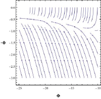
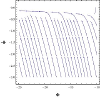
   (a)  (b)  (c)

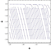
   Figure 1: Direction fields on the $(\Phi,\dot{\Phi})$ phase space for negative values of $\Phi$ and various values of $\beta$: (a) $\beta=-0.1$, (b) $\beta=-0.3$, and (c) $\beta=-1$.

2. $\Phi_{i}>2$. The direction fields on this approximative analysis are shown in Fig. 2. We notice the existence of an attractor line for different values of $\beta$. This indicates the existence of the slow-roll regime. The attractor line shows $\Phi$ decreasing with time. If we extrapolate the observed behavior of this line, we expect the field $\Phi$ to reach values for which the condition $\frac{\Theta}{\Phi}\ll 1$ will eventually break down. This is a necessary condition for inflation to cease. However, the condition $\Phi\gg 1$ will also be violated and when this happens, we cannot rely on Eqs. (133) to properly describe our system.

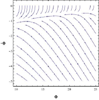
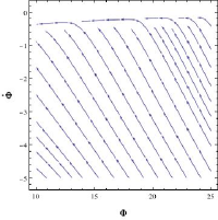
   (a)  (b)  (c)

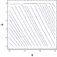
   Figure 2: Direction fields on the $(\Phi,\dot{\Phi})$ phase space for positive values of $\Phi$ and various values of $\beta$: (a) $\beta=0.1$, (b) $\beta=0.3$,   (c) $\beta=1$.

We conclude that inflation happens in this scenario, but we cannot be decisive if it ends or not. In order to achieve a definitive answer, the equations should be studied without any approximation. This is done in the next section.

IV.2 Analysis of the complete equations — Assessing the existence of an end to inflation

In order to check if and how inflation ends in our model, we have to analyze Eqs. (114) and (115) with no approximations. We have to consider a set of initial conditions for $\Phi$ and $\Theta$ that are consistent with inflation (i.e. $\Theta_{i}\ll\Phi_{i}$) and follow the evolution of the variables. The end of inflation will be characterized by the violation of condition $\Theta\ll\Phi$. We also expect the dynamics of the auxiliary fields will come to an end, allowing the universe to enter a radiation-dominated era. These conditions are achieved if we find attractors (fixed points) for Eqs. (114) and (115) on which the condition $\Theta\ll\Phi$ is not satisfied.

IV.2.1 Fixed points

The fixed points of the system are found when

$$\frac{\Theta}{\Phi}\left(\frac{-3J+\Phi-6\beta h_{c}\Theta}{J+\left(\Phi-2\right)-3\beta\left(\frac{\Theta}{\Phi}\right)^{2}}\right) =0,$$ (136)

$$\frac{\Phi-J}{2\beta}-3h_{c}\Theta+2\frac{\Theta^{2}}{\Phi^{2}}\left(\frac{-3J+\Phi-6\beta h_{c}\Theta}{J+\left(\Phi-2\right)-3\beta\left(\frac{\Theta}{\Phi}\right)^{2}}\right) =0.$$ (137)

One of the fixed points is obtained when $\Theta=0$ and $J=\Phi\Rightarrow\Phi=1$. However, if we start in a region where $\Phi\gg 1$, then we have to cross the critical region $\Phi=2$. This is possible if and only if $\Theta=0$ at the same time when $\Phi=2$, otherwise, $J$ becomes complex. Besides, for this very same reason, when going from $\Phi=2$ to $\Phi=1$, $\Theta$ has to be null. However, when $\left(\Phi,\Theta\right)=\left(2,0\right)$, $\dot{\Phi}=0$ and $\dot{\Theta}>0$ [see Eqs. (114] and (115)), showing that the trajectory tends to keep $\Phi$ unchanged and to increase the values of $\Theta$, the trajectory does not move toward the point $\left(1,0\right)$. This is what makes the region of the configuration space $\Phi<2$ problematic for our system, and for this reason, this fixed point will be discarded.

We find another fixed point when

$$\begin{cases}-3J+\Phi_{E}-6\beta h_{c}\Theta_{E}=0\\ -J+\Phi_{E}-6\beta h_{c}\Theta_{E}=0\end{cases}.$$ (138)

In this case,

$$J=0\Rightarrow\Theta_{E}=\pm\sqrt{\frac{\Phi_{E}}{2\beta}\left(\Phi_{E}-2\right)^{2}}$$ (139)

and

$$\Phi_{E}=6\beta h_{c}\Theta_{E}.$$ (140)

Considering that $\Phi_{E}$ and $\beta$ have the same sign and $h_{c}$ is positive, the minus sign on Eq. (139) has to be neglected.

Replacing Eq. (139) in Eq. (140) shows that $\Phi_{E}$ is found as a solution of the following equation:

$$\left(\Phi_{E}-\frac{6}{5}\right)\left(\Phi_{E}-2\right)^{3}\beta=\frac{8\Phi_{E}^{3}}{15}.$$ (141)

This is a fourth-order equation for $\Phi_{E}$, which presents four solutions. Two of them are complex solutions and for this reason they will be neglected. The other two solutions are real. One of them, however, is bound to be less than $6/5$, for any value of $\beta$ — see Fig. 3. As has been discussed before, the region $\Phi<2$ is not suitable for our system: we are left with only one of the four solutions — the upper curve in Fig. 3.

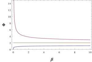
Figure 3: Real solutions $\Phi_{E}$ of Eq. (141) and the function $\Phi=2$ as a function of $\beta$.

First, we check consistency with the Hubble function, which is rewritten as:

$$h_{c}^{2}\left(\Phi_{E},\Theta_{E}\right)=\frac{1}{24}\frac{1}{\Phi_{E}^{2}}\left(\Phi_{E}-\frac{6}{5}\right)\left(\Phi_{E}-2\right).$$ (142)

For $\Phi_{E}>2$, $h_{c}^{2}>0$ and $h_{c}$ is real and positive.

Second, we have to check if the denominator $D\left(\Phi,\Theta\right)\equiv J+\left(\Phi-2\right)-3\beta\left(\frac{\Theta}{\Phi}\right)^{2}$ — see Eqs. (136) and (137) — does not vanish at the fixed point. We have

$$D\left(\Phi_{E},\Theta_{E}\right)=-\frac{\left(\Phi_{E}-2\right)\left(\Phi_{E}-6\right)}{2\Phi}$$ (143)

This expression shows we have a singularity if $\Phi_{E}=6$. This singularity can be avoided if we correctly choose the value of the parameter $\beta$. Equation (141) can be used to invert $\beta$ in terms of $\Phi_{E}$ :

$$\beta=\frac{8\Phi_{E}^{3}}{15\left(\Phi_{E}-\frac{6}{5}\right)\left(\Phi_{E}-2\right)^{3}}.$$ (144)

If we set $\Phi_{E}=6$, then $\beta=0.375$. If we choose $\beta\neq 0.375$, then for $\Phi_{E}>2$ we have no problem of singularities with $D\left(\Phi_{E},\Theta_{E}\right)$.

In the third place, we check if the scale factor decelerates at the fixed point, allowing inflation to cease and the universe to change from a de Sitter–type phase to a decelerated expansion. From Eq. (117), we find

$$\frac{\ddot{a}}{a}=-\frac{1}{48\Phi_{E}^{2}}\left(\Phi_{E}-6\right)\left(\Phi_{E}-2\right).$$

Consequently, if $2<\Phi_{E}<6$, we have an acceleration of the scale factor, while for $\Phi_{E}>6$ we have a deceleration. Therefore, in order to have a suitable fixed point which could eventually lead to a good model of inflation we are forced to choose $0<\beta<0.375$, according to Eq. (144).

IV.2.2 Stability of the fixed point

At last, we have to check if the fixed point is an attractor. In principle, this can be done by assessing the Lyapunov coefficients. These are obtained as the eigenvalues $\lambda_{\pm}$ of the matrix

$$M=\left(\begin{array}[]{cc}\frac{\partial f}{\partial\Phi}&\frac{\partial f}{\partial\Theta}\\ \frac{\partial g}{\partial\Phi}&\frac{\partial g}{\partial\Theta}\end{array}\right)_{\begin{array}[]{c}\Phi=\Phi_{E}\\ \Theta=\Theta_{E}\end{array}},$$ (145)

whose elements are calculated from Eqs. (114) and (115). Since we have a $2\times 2$ matrix, it is immediate that:

$$\lambda_{\pm}=\frac{1}{2}\left[\left(\frac{\partial f}{\partial\Phi}+\frac{\partial g}{\partial\Theta}\right)\pm\sqrt{\left(\frac{\partial f}{\partial\Phi}+\frac{\partial g}{\partial\Theta}\right)^{2}-4\left(\frac{\partial f}{\partial\Phi}\frac{\partial g}{\partial\Theta}-\frac{\partial g}{\partial\Phi}\frac{\partial f}{\partial\Theta}\right)}\right]_{\begin{array}[]{c}\Phi=\Phi_{E}\\ \Theta=\Theta_{E}\end{array}}$$

However, the partial derivatives in the above expression diverge, making the Lyapunov coefficients analysis difficult to be implemented. In order to circumvent this problem, we have to look for numerical solutions and see if an attractor appears.

We performed numerical calculations in order to build the direction fields on the $(\Phi,\dot{\Phi})$ phase space and checked the existence of an attractor on this space. The procedure for building these curves was the following:

• we started with initial conditions $\left(\Phi_{i},\Theta_{i}\right)$ and a fixed value $\beta$ and found numerical solutions $\left(\Phi_{i}\left(t\right),\Theta_{i}\left(t\right)\right)$;

• by plotting the curves $\Phi_{i}\left(t\right)$, we verified that $\Phi_{i}\left(t\right)$ is monotonous in time, so the inverse relation $t_{i}=t\left(\Phi_{i}\right)$ was obtained;

• from the solutions $\Theta_{i}\left(t\right)$, we found $\Theta\left(\Phi\right)=\Theta_{i}\left(t\left(\Phi_{i}\right)\right)$;

• we derived Eq. (114) with respect to time. This led to a second order equation for $\Phi$, i.e. $\ddot{\Phi}=\ddot{\Phi}\left(\Phi,\dot{\Phi},\Theta,\dot{\Theta}\right)$;

• we replaced $\ddot{\Phi}$ by $\frac{d\dot{\Phi}}{d\Phi}\dot{\Phi}$, $\dot{\Theta}$ by $\dot{\Theta}\left(\Phi,\Theta\left(\Phi\right)\right)$ and $\Theta$ by $\Theta\left(\Phi\right)$ thus obtaining $\frac{d\dot{\Phi}}{d\Phi}=\frac{1}{\dot{\Phi}}F\left(\Phi,\dot{\Phi}\right)$, where $F\left(\Phi,\dot{\Phi}\right)=\ddot{\Phi}\left(\Phi,\dot{\Phi},\Theta\left(\Phi\right),\dot{\Theta}\left(\Phi,\Theta\left(\Phi\right)\right)\right)$;

• the direction fields on the $(\Phi,\dot{\Phi})$ phase space were plotted.

The result is presented in Fig. 4 for $\beta=0.1$. Other values of $\beta$ produce similar graphs; for this reason, they were not displayed in the text. The graph in Fig. 4 displays an attractor line along which $\Phi$ decreases slowly (toward corresponding smaller values of $\dot{\Phi}$). So the slow-roll regime takes place even for the nonapproximate equations. As $\Phi$ approaches $\sim 5$, the attractor line changes drastically: $\Phi$ practically stops decreasing and $\dot{\Phi}$ increases very fast. The trajectory diverges in the phase space and no attractor can be identified. The conclusion is straightforward: there is an inflationary period but the trajectories do not lead to an attractor; hence, the dynamics of the auxiliary fields does not seem to end and the model does not provide a satisfactory end for the inflationary period. No graceful exit can be identified by the numerical solutions.

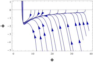
Figure 4: Direction fields on the $(\Phi,\dot{\Phi})$ phase space for the complete set of equations with $\beta=0.1$.

We conclude this section by stating that the Starobinsky-Podolsky model analyzed in the Einstein frame in the Palatini formalism does not provide a satisfactory model for inflation.

V Final remarks

This paper was dedicated to construct the scalar-multitensorial equivalent of higher-order $f\left(R,\nabla R,\dots\right)$ theories of gravity in the Einstein frame. The work was performed in the metric and Palatini formalisms pointing out the differences and similarities. The main difference between these formulations is that in the metric approach there is a clear kinetic structure for the scalar field $\tilde{\Phi}$, whereas in the Palatini approach this structure is absent. This is explicitly verified in the differences between the effective energy-momentum tensors and between the scalar field equations of both approaches. In addition, we also thoroughly studied the particular case of the Starobinsky-Podolsky model in the Einstein frame and characterized its effective energy-momentum tensor in terms of a fluid description, where a shearless imperfect fluid is obtained in the metric approach, while a perfect fluid is obtained in Palatini formalism. This completes the development started in Ref. PRD2016 .

An important point to be emphasized is that although the higher-order $f\left(R,\nabla R,\dots\right)$ theories have an apparently similar form to the $f\left(R\right)$ theories in the Einstein frame, they differ substantially due to the structure of the potential $\tilde{U}$. While in $f\left(R\right)$ theories the potential $\tilde{U}$ depends only on the scalar field, in higher-order models, $\tilde{U}$ has a much more complex structure depending on the extra fields $\left\{\Phi,\phi_{\mu},\dots,\phi_{\mu_{1}\dots\mu_{n}}\right\}$ and its covariant derivatives. However, even taking into account the complexity of the potential $\tilde{U}$, the $f\left(R,\nabla R,\dots\right)$-like theories are simplified considerably when rewritten in Einstein frame. This is particularly true in the situation where the higher-order terms are small corrections to the Einstein-Hilbert (or Starobinsky) action and in this case the potential $\tilde{U}$ can be treated in a perturbative way.

There are several cases where it is convenient to describe the $f\left(R,\nabla R,\dots\right)$ theories in Einstein frame. In particular, an important case to be analyzed is the study and description of ghosts. Following an approach analogous to that in Ref. Hindawi1996 , one can study in which higher-order theories and under which conditions the pathologies involving ghosts are avoided.

Another interesting case takes place in inflationary cosmology. Usually, inflationary models based on modified gravity are more easily described in the Einstein frame. For example, Starobinsky’s inflation Starobinsky1980 is widely studied through its scalar-tensorial version. In Sec. IV, we explored the possibility of generating inflation through Starobinsky-Podolsky gravity in the Palatini formalism. We showed that the extra (vector) field is able to engender an inflationary regime for a wide range of initial conditions. However, this regime does not end in a satisfactory way: it does not lead to a hot-big-bang type of dynamics. Some possibilities to circumvent this problem are to include even higher-order terms, to introduce extra new fields or even to consider nonminimal couplings. Finally, it is worth mentioning that a similar but more involved analysis was done in StaPodInf ; this paper considered Starobinsky-Podolsky inflation in the metric formalism and showed a graceful exit is possible for the model.

- (1) D. M. Scolnic et al., Astrophys. J. 859, 111 (2018).
- (2) Planck Collaboration, [arXiv:1807.06211].
- (3) Y. Akrami et al., (Planck Collaboration), [arXiv:1807.06205].
- (4) Y. Akrami et al., (Planck Collaboration), [arXiv:1807.06209].
- (5) T. M. C. Abbott et al. (DES Collaboration), Phys. Rev. D 98, 043526 (2018)..
- (6) R. D. Peccei and H. R. Quinn, Phys. Rev. D 16, 1791 (1977).
- (7) M. Sasaki, Prog. Theor. Phys. 72, 1266 (1984).
- (8) S. Alexander, R. Brandenberger, and J. Froehlich, arXiv:1609.06920 [hep-th].
- (9) D. J. E. Marsh, Phys. Rep. 643, 1 (2016).
- (10) K. Saikawa, Proc. Sci., EPS-HEP2017 (2017) 083 [arXiv:1709.07091 [hep-th]].
- (11) L. Roszkowski, E. M. Sessolo, and S. Trojanowski, Rep. Prog. Phys. 81, 066201 (2018).
- (12) L. Berezhiani, and J. Khoury, Phys. Rev. D 92, 103510 (2015).
- (13) E. G. M. Ferreira, G. Franzmann, R. Brandenberger, and J. Khoury, arXiv:1810.09474.
- (14) S. Alexander, E. McDonough, and D. N. Spergel, J. Cosmol. Astropart. Phys. 05 (2018) 003.
- (15) E. Aprile et al. Phys. Rev. D 90, 062009 (2014).
- (16) D. S. Akerib et al. Phys. Rev. Lett. 118, 021303 (2017).
- (17) S. M. Carroll, W. H. Press, and E. L. Turner, Ann. Rev. Astron. Astrophys. 30, 499 (1992).
- (18) L. Amendola and S. Tsujikawa, Dark Energy. Theory and Observations (Cambridge University Press, Cambridge, England, 2010).
- (19) R. R. Caldwell, R. Dave, and P. J. Steinhardt, Phys. Rev. Lett. 80, 1582 (1998).
- (20) S. M. Carroll, Phys. Rev. Lett. 81, 3067 (1998).
- (21) S. Tsujikawa, Classical Quantum Gravity 30, 214003 (2013).
- (22) T. Chiba, T. Okabe, and M. Yamaguchi, Phys. Rev. D 62, 023511(2000).
- (23) C. Armendariz-Picon, V. F. Mukhanov, and P. J. Steinhardt, Phys. Rev. D 63, 103510 (2001).
- (24) R. R. Cuzinatto, L. G. Medeiros, and E. M. de Morais, Astropart. Phys. 73, 52 (2016).
- (25) R. R. Cuzinatto, L. G. Medeiros, E. M. de Morais, and R. H. Brandenberger, Astropart. Phys. 103, 98 (2018).
- (26) R. Brandenberger, R. R. Cuzinatto, J. Fröhlich, and R. Namba, J. Cosmol. Astropart. Phys. 02 (2019) 043.
- (27) M. C. Bento, O. Bertolami, and A. A. Sen, Phys. Rev. D 66, 043507 (2002).
- (28) D. Bertacca, N. Bartolo, and S. Matarrese, Adv. Astron. 2010, 1 (2010).
- (29) R. R. R. Reis, I. Waga, M. O. Calvão, and S. E. Jorás, Phys. Rev. D 68, 061302(R) (2003).
- (30) E. V. Linder and D. Huterer, Phys. Rev. D 72, 043509 (2005).
- (31) S. Capozziello and M. Francaviglia, Gen. Relativ. Gravit. 40, 357 (2008).
- (32) T. P. Sotiriou and V. Faraoni, Rev. Mod. Phys. 82, 451 (2010).
- (33) S. Nojiri and S. D. Odintsov, Phys. Rep. 505, 59 (2011).
- (34) S. Nojiri, S. D. Odintsov, and V. K. Oikonomou, Phys. Rept. 692, 1 (2017).
- (35) E. N. Saridakis and M. Tsoukalas, Phys. Rev. D 93, 124032 (2016).
- (36) P. Bueno, P. A. Cano, O. Lasso A., and P. F. Ramirez, J. High Energy Phys. 04 (2016) 028.
- (37) S. Jhingan, S. Nojiri, S.D. Odintsov, M. Sami, I. Thongkool, and S. Zerbini, Phys. Lett. B 663, 424 (2008).
- (38) Q. Exirifard and M. M. Sheikh-Jabbari, Phys. Lett. B 661, 158 (2008).
- (39) S. Nojiri and S. D. Odintsov, Phys. Rev. D 68, 123512 (2003).
- (40) S. Nojiri and S. D. Odintsov, Int. J. Geom. Methods Mod. Phys. 04, 115 (2007).
- (41) S. Nojiri and S. D. Odintsov, Phys. Lett. B 659, 821 (2008).
- (42) T. Biswas, T. Koivisto, and A. Mazumdar, J. Cosmol. Astropart. Phys. 11 (2010) 008.
- (43) T. Biswas, E. Gerwick, T. Koivisto, and A. Mazumdar, Phys. Rev. Lett. 108, 031101 (2012).
- (44) T. Biswas and S. Talaganis, Mod. Phys. Lett. A 30, 1540009 (2015).
- (45) R. R. Cuzinatto, C. A. M. de Melo, L. G. Medeiros, and P. J. Pompeia, Eur. Phys. J. C 53, 99 (2008).
- (46) A. L. Berkin, and K. Maeda, Phys. Lett. B 245, 348 (1990).
- (47) S. Gottlöbert, V. Möller, and H.-J. Schmidt, Astron. Nachr. 312, 291 (1991).
- (48) L. Amendola, A. B. Mayert, S. Capozziello, S. Gottlöbert, V. Möller, F. Occhionero, and H.-J. Schmidt, Classical Quantum Gravity 10, L43 (1993).
- (49) M. Lihoshi, J. Cosmol. Astropart. Phys. 02 (2011) 022.
- (50) G. A. Diamandis, B. C. Georgalas, K. Kaskavelis, A. B. Lahanas, and G. Pavlopoulos, Phys. Rev. D 96, 044033 (2017).
- (51) A. S. Koshelev, L. Modesto, L. Rachwal, and A. A. Starobinsky, J. High Energ. Phys. 11 (2016) 067.
- (52) A. S. Koshelev, K. S. Kumar, and A. A. Starobinsky, J. High Energ. Phys. 03 (2018) 071.
- (53) J. Edholm, Phys. Rev. D 95, 044004 (2017).
- (54) D. Chialva and A. Mazumdar, Mod. Phys. Lett. A 30, 1540008 (2015).
- (55) L. Modesto, Phys. Rev. D 86, 044005 (2012).
- (56) I. L. Shapiro, Phys. Lett. B 744, 67 (2015).
- (57) L. Modesto and I. L. Shapiro, Phys. Lett. B 755, 279 (2016).
- (58) N. Ohta, R. Percacci, and A. D. Pereira, Phys. Rev. D 97, 104039 (2018).
- (59) D. Langlois and K. Noui, J. Cosmol. Astropart. Phys. 07 (2016) 016.
- (60) J. BenAchour, D. Langlois, and K. Noui, Phys. Rev. D 93, 124005 (2016).
- (61) D. Langlois and K. Noui, J. Cosmol. Astropart. Phys. 02 (2016) 034.
- (62) B. Paul, Phys. Rev. D 96, 044035 (2017).
- (63) D. S. Kaparulin, S. L. Lyakhovich, and A. A. Sharapov, Eur. Phys. J. C 74, 3072 (2014).
- (64) R. R. Cuzinatto, C. A. M. de Melo, L. G. Medeiros, and P. J. Pompeia, Phys. Rev. D 93, 124034 (2016).
- (65) M. S. Ruf and C. F. Steinwachs, Phys.Rev. D 97, 044049 (2018).
- (66) M. S. Ruf and C. F. Steinwachs, Phys. Rev. D 97, 044050 (2018).
- (67) N. Ohta, Prog. Theor. Exp. Phys. 2018, 033B02 (2018).
- (68) J. D. Barrow and S. Cotsakis, Phys. Lett. B 214, 515 (1988).
- (69) B. Witt, Phys. Lett. B 145, 176 (1984).
- (70) V. I. Alfonso, C. Bejarano, J. B. Jiménez, G. J. Olmo, and E. Orazi, Classical Quantum Gravity 34, 235003 (2017).
- (71) A. A. Starobinsky, Phys. Lett. B 91, 99 (1980).
- (72) R. Aldrovandi, R. R. Cuzinatto, and L. G. Medeiros, Eur. Phys. J. C 58, 483 (2008).
- (73) R. Aldrovandi, R. R. Cuzinatto, and L. G. Medeiros, Int. J. Mod. Phys. D 17, 857 (2008).
- (74) R. Costa, R. R. Cuzinatto, E. M. G. Ferreira, and G. Franzmann, arXiv:1705.03461 [gr-qc] [Int. J. Mod. Phys. D (to be published)].
- (75) Ya. B. Zeldovich, and A. A. Starobinsky, Zh. Eksp. Teor. Fiz. 61, 2161 (1971) [Sov. Phys. JETP 34, 1159 (1972)].
- (76) R. R. Cuzinatto, L. G. Medeiros, and P. J. Pompeia, J. Cosmol. Astropart. Phys. 02 (2019) 055.
- (77) A. R. R. Castellanos, F. Sobreira, I. L. Shapiro, and A. A. Starobinsky, J. Cosmol. Astropart. Phys. 12 (2018) 007.
- (78) R. M. Wald, General Relativity (University of Chicago Press, Chicago,1984).
- (79) C. M. Will, Theory and Experiment in Gravitational Physics (Cambridge University Press, New York, 1981).
- (80) R. R. Cuzinatto, C. A. M. de Melo, and P. J. Pompeia, Ann. Phys. 322, 1211 (2007).
- (81) R. R. Cuzinatto, C. A. M. de Melo, L. G. Medeiros, and P. J. Pompeia, Astrophys. Space Sci. 332, 201 (2011).
- (82) R. R. Cuzinatto, C. A. M. de Melo, L. G. Medeiros, and P. J. Pompeia, Gen. Relativ. Gravit. 47, 29 (2015).
- (83) G. F. R. Ellis, R. Maartens, and M. A. H. MacCallum, Relativistic Cosmology (Cambridge University Press, Cambridge, England 2012).
- (84) A. Hindawi, B. A. Ovrut, and D. Waldram, Phys. Rev. D 53, 5597 (1996).