CLUMPY v3: $\gamma$-ray and $\nu$ signals from dark matter at all scales

Abstract

We present the third release of the CLUMPY code for calculating $\gamma$-ray and $\nu$ signals from annihilations or decays in dark matter structures. This version includes the mean extragalactic signal with several pre-defined options and keywords related to cosmological parameters, mass functions for the dark matter structures, and $\gamma$-ray absorption up to high redshift. For more flexibility and consistency, dark matter halo masses and concentrations are now defined with respect to a user-defined overdensity $\Delta$. We have also made changes for the user’s benefit: distribution and versioning of the code via git, less dependencies and a simplified installation, better handling of options in run command lines, consistent naming of parameters, and a new Sphinx documentation at http://lpsc.in2p3.fr/clumpy/.

PROGRAM SUMMARY

Program Title: CLUMPY
Programming language: C/C++
Computer: PC and Mac
Operating system: UNIX(Linux), MacOS X
RAM: between 500 MB and 10 GB depending on the size or resolution of requested 2D skymaps
Keywords: cosmology, dark matter, indirect detection, $\gamma$-rays, $\nu$
Classification: 1.1, 1.7, 1.9
External routines/libraries: GSL (http://www.gnu.org/software/gsl), cfitsio (http://heasarc.gsfc.nasa.gov/fitsio/fitsio.html), CERN ROOT (http://root.cern.ch; optional, for interactive figures and stochastic simulation of halo substructures), GreAT (http://lpsc.in2p3.fr/great; optional, for MCMC Jeans analyses)
Nature of problem: Calculation of the $\gamma$-ray and $\nu$ signals from dark matter annihilation/decay at any redshift $z$.
Solution method: New in this release: Numerical integration of moments (in redshift and mass) of the mass function, absorption, and intensity multiplier (related to the DM density along the line of sight).
Restrictions: Secondary radiation from dark matter leptons, which depends on astrophysical ingredients (radiation fields in the Universe) is the last missing piece to provide a full description of the expected signal.
Running time: Depending on user-defined choices, primarily on substructure modelling and numeric precision $\epsilon$: For instance, it takes $\lesssim$ 3 s to compute an energy spectrum of the extragalactic intensity from annihilation without halo substructure and $\epsilon=0.01$. Considering one level of substructure or choosing $\epsilon=10^{-3}$ doubles the running time.

1 Introduction

Indirect signatures of dark matter (DM) annihilation or decay are being actively sought for in the fluxes of charged cosmic rays [1], $\gamma$-rays [2] and neutrinos [3, 4]. The CLUMPY code has been developed over the last decade to provide a public tool to estimate the DM-induced fluxes of $\gamma$-rays and neutrinos, in a large variety of objects and user-defined configurations. Our knowledge about the masses and shapes of DM structures throughout the Universe is largely dependent on cosmological simulations, which all provide similar but still different parametrisations of the DM properties; CLUMPY allows the user to easily switch and combine these parametrisations and to efficiently compute resulting $\gamma$-ray or neutrino ($\nu$) signals for indirect DM searches. The goal of CLUMPY is to eventually provide an unified and comprehensive calculation of the exotic signal at both the Galactic and extragalactic scales.

The first release of the code, published in [5], focused on the optimised calculation of the so-called astrophysical $J$-factor, a key quantity for indirect detection studies at the Galactic scale. The code could simply provide the $J$-factor of a user-defined halo, or compute $J$-factor maps in the flat sky approximation of the Galactic halo or of any isolated halo, including substructures. This first release was used in [6, 7, 8, 9, 10].

In [11], a second and much more complete release of the code was delivered to the community. From then, CLUMPY included the source $\gamma$-ray and $\nu$ spectra computed from [12] that allow to compute not only the $J$-factors, but the actual exotic prompt radiation from DM annihilation or decay. Another important new feature of that release was a Jeans analysis module to compute the DM profile of dwarf spheroidal galaxies, prime targets of indirect DM detection, from their kinematic data and to propagate the uncertainties to the $J$-factors (e.g., [13, 14, 15, 16]). Using HEALPix, the possibility to compute full skymaps was also included and largely used in [17].

Up to now, the calculations implemented in CLUMPY have been only valid at the Galactic scale and for the local Universe, where cosmology and absorption can be ignored. This paper describes the third release of CLUMPY, which now also includes the mean extragalactic contribution to the exotic $\gamma$-rays and neutrinos in a flat $\Lambda$CDM universe, used to produce the results of [19]. This addition is the missing piece to provide, within the same framework, a tool to consistently compare all potential DM targets on the Galactic and extragalactic scale.

The new extragalactic physics included into CLUMPY is described in §2 of this paper. §3 presents the main additions brought to the code in order to effectively implement this physics, while some new, more minor features included in this release are summarised in §4. New parameters and keywords are described in §5. CLUMPY has several library dependencies that have made the previous release quite complex to install. For this third version of the code, the installation process has been greatly simplified, making some dependencies optional as described in §6.

2 Average $\gamma$-ray and $\nu$ fluxes from extragalactic DM

The extragalactic differential $\gamma$-ray or $\nu$ intensity of annihilating Majorana DM, averaged over the whole sky, is given by (see, e.g., [20, 21, 22, 23, 24, 25])

$$I_{\rm ann}(E_{\gamma,\nu})\;=\;\left\langle\frac{\mathrm{d}\Phi}{\mathrm{d}E_{\gamma,\nu}\,\mathrm{d}\Omega}\right\rangle_{\rm sky}\;=\;\frac{\overline{\varrho}^{2}_{\mathrm{DM},\,0}\,\langle\sigma v\rangle}{8\pi\,m_{\chi}^{2}}$$ (1)

$$\times \int\limits_{0}^{z_{\mathrm{max}}}c\,\mathrm{d}z\,\frac{(1+z)^{3}}{H(z)}\left\langle\delta^{2}(z)\right\rangle\left.\frac{\mathrm{d}N^{{\gamma,\nu}}_{\mathrm{source}}}{\mathrm{d}E_{\mathrm{e}}}\right|_{E_{\mathrm{e}}=(1+z)E_{\gamma,\nu}}\times e^{-\tau(z,\,E_{\gamma})}\,,$$

with $E_{\gamma,\nu}$ the observed energy, $\Phi$ the flux, $\mathrm{d}\Omega$ the elementary solid angle, $c$ the speed of light, and $\overline{\varrho}_{\mathrm{DM},\,0}$ the DM density of the Universe today. $H(z)$ is the Hubble constant at redshift $z$, $m_{\chi}$ the DM candidate mass, and $\langle\sigma v\rangle$ the velocity averaged annihilation cross section. $\mathrm{d}N^{\gamma,\nu}_{\mathrm{source}}/\mathrm{d}E_{\mathrm{e}}$ is the differential $\gamma$-ray/$\nu$ yield per annihilation evaluated at $E_{\rm e}=(1+z)E_{\gamma}$, corresponding to a photon at $E_{\gamma}$ today, and $\tau(z,\,E_{\gamma})$ describes the optical depth of the Universe to $\gamma$-rays of GeV to beyond-TeV energies. Finally, $\langle\delta^{2}\rangle=1+\mathrm{Var}(\delta)$ is the intensity multiplier related to the DM inhomogeneity $\delta$.

For decaying DM with lifetime $\tau_{\mathrm{DM}}$, the intensity is given by

$$I_{\rm decay}(E_{\gamma,\nu})\;=\;\frac{\overline{\varrho}_{\mathrm{DM},\,0}}{4\pi\,\tau_{\mathrm{DM}}\,m_{\chi}}$$ (2)

$$\times \int\limits_{0}^{z_{\mathrm{max}}}c\,\mathrm{d}z\,\frac{1}{H(z)}\,\left.\frac{\mathrm{d}N^{{\gamma,\nu}}_{\mathrm{source}}}{\mathrm{d}E_{\mathrm{e}}}\right|_{E_{\mathrm{e}}=(1+z)E_{\gamma,\nu}}\times e^{-\tau(z,\,E_{\gamma})}\,.$$

As of now, CLUMPY only accounts for the prompt $\gamma$-ray emission, given by the above equations. The diffuse secondary emission, produced by the inverse Compton scattering (ICS) of DM-produced $e^{+/-}$ with CMB photons or other radiation fields [26, 27], is not yet implemented. The spectrum of these up-scattered photons peaks at lower energies compared to the prompt $\gamma$-ray emission (see, e.g., figure 1 of [28]); accounting for those photons would change the spectra produced by CLUMPY at energies below $10^{-2}m_{\chi}$.

3 Implementation in CLUMPY: new and updated functions

3.1 New module cosmo.cc

Computation of the extragalactic intensity as given by Eq. (1) requires accounting for the cosmology. This is done in a new module, cosmo.cc, which contains all cosmology-related functions, from the computation of the various cosmological distances to the evaluation of the halo mass function required by the intensity multiplier $\langle\delta^{2}(z)\rangle$, Eq. (3) below. A large fraction of the functions included in this module are a translation into C of Eiichiro Komatsu’s very useful Cosmology Routine Library in Fortran.

3.1.1 Cosmological distances

There are several ways to define distances in cosmology, whether one is interested in the i) distance between two objects along the line of sight (comoving distance), ii) the transverse distance between two objects at the same redshift (transverse comoving distance), iii) the physical size of an object given its observed angular size (angular diameter distance), or iv) the distance to link an observed flux to the intrinsic luminosity of a source (luminosity distance). These well-known definitions depend on the cosmological parameters and redshift and are not repeated here (see, e.g., [30]), but have been included in the cosmo.cc.

3.1.2 Intensity multiplier $\langle\delta^{2}(z)\rangle$ of annihilating DM

The quantity $\langle\delta^{2}(z)\rangle$ is computed according to the halo model approach [20, 31, 25]. In this setup, the intensity multiplier from the inhomogeneous Universe is written as

$$\left\langle\delta^{2}(z)\right\rangle=\frac{1}{\overline{\varrho}^{2}_{\mathrm{m,0}}}\;\int\mathrm{d}M\frac{\mathrm{d}n}{\mathrm{d}M}(M,z)\times\mathcal{L}(M,z)\,,$$ (3)

where $\overline{\varrho}_{\mathrm{m,\,0}}$ is today’s mean total matter density, ${\mathrm{d}n}/\mathrm{d}M$ the halo mass function, and $\mathcal{L}(M,z)$ the one-halo luminosity.

The halo mass function

The number density of haloes ${\mathrm{d}n}/{\mathrm{d}M}$ in a given mass range at redshift $z$ depends on the variance $\sigma$ of the density fluctuations and on the multiplicity function $f(\sigma,\,z)$ that encodes nonlinear structure formation,

$$\frac{\mathrm{d}n}{\mathrm{d}M}(M,\,z)=f(\sigma,z)\;\frac{\overline{\varrho}_{\rm m,0}}{M}\,\frac{\mathrm{d}\ln\sigma^{-1}}{\mathrm{d}M}\,.$$ (4)

The variance $\sigma$ is calculated from the linear matter power spectrum, $P_{\rm lin}(k,z=0)$, according to

$$\sigma^{2}(M,\,z)=\frac{D(z)^{2}}{2\pi^{2}}\int P_{\rm lin}(k,z=0)\,\widehat{W}^{2}(kR)\,k^{2}\,\mathrm{d}k\,,$$ (5)

with $R=[M/(\gamma_{\rm f}\,\overline{\varrho}_{\rm m,0})]^{1/3}$ the comoving scale radius of a collapsing sphere containing the mass $M$. Different shapes of the sphere can be selected (see Tab. 2), expressed in $k$-space by

$$\widehat{W}(kR) =3\,(kR)^{-3}\,[\sin(kR)-kR\,\cos(kR)],\;\gamma_{\rm f}=\frac{4\pi}{3};$$ (top-hat)

$$\widehat{W}(kR) =\exp[-(kR)^{2}/2],\;\gamma_{\rm f}=(2\pi)^{3/2};$$ (Gaussian window)

$$\widehat{W}(kR) =1-\theta(kR-1),\;\gamma_{\rm f}=6\pi^{2}\,; k$$ (sharp- filter)

with $\theta$ the Heaviside step-function. CLUMPY is interfaced with the CLASS code [32] to compute $P_{\rm lin}(k,z=0)$. The growth factor $D(z)=g(z)/g(z=0)$, defined from

$$g(z)=\frac{5}{2}\times\frac{8\pi G}{3}\overline{\varrho}_{\rm m,0}\times H(z)\,\int_{z}^{\infty}\frac{1+z^{\prime}}{H^{3}(z^{\prime})}\,\mathrm{d}z^{\prime}\,,$$ (6)

then allows to compute the variance at any redshift ($G$ is the gravitational constant).

The multiplicity function $f(\sigma,z)$ is generally fitted to numerical simulations. CLUMPY includes the parametrisations from a variety of simulations, considering only DM or including baryons and relying on different cosmologies. The available parametrisations are listed in Tab. 2 and the user may select any one of these with a corresponding keyword (see §5 for details).

The comoving one-halo luminosity

The other term required by the intensity multiplier is the halo luminosity, defined to be

$$\mathcal{L}(M_{\Delta},z)=\int\mathrm{d}V\,\rho^{2}_{\mathrm{halo}}=4\pi\int_{0}^{R_{\Delta}}\mathrm{d}r\,r^{2}\,\rho^{2}_{\mathrm{halo}}\,.$$ (7)

It depends on the halo mass $M_{\Delta}$ (which defines its size $R_{\Delta}$, see §4.2), on the halo density profile $\rho_{\mathrm{halo}}(r;\,\rho_{-2},\,r_{-2})$, and on the mass-concentration relation $c_{\Delta}(M_{\Delta},z):=R_{\Delta}/r_{-2}$ which is required to determine the normalisation of the profile given the halo mass. All mass-concentrations available in CLUMPY are now implemented with their proper redshift-scaling. The halo luminosity has existed in CLUMPY since the first release and is defined in the clumps.cc module (see the previous release articles [5, 11]).

3.1.3 Main functions

• dh_{c, trans, a, l}: a set of functions returning, for a given cosmology and redshift, the comoving (c), the transverse comoving (trans), the angular diameter (a) and the luminosity (l) distances.

• get_pk: for a given cosmology, loads the matter power spectrum from an existing file, the name of which should match a pattern obtained from the cosmological parameters. If the file does not exist, the function calls compute_class_pk to compute $P_{\rm lin}(k)$ using CLASS (which should have been previously installed by the user).

• growth_factor: computes the linear growth rate $D(z)$, for a given redshift, using either the exact analytical solution of Eq. (6) or the approximate (and faster to compute) formula of [33], depending on the user’s choice.

• mf_*: a set of functions returning the multiplicity function obtained by various authors from various simulations, as listed in Tab. 2. The asterisk is to be replaced by the authors or simulation name.

• compute_massfunction: returns a vector of tabulated values of the mass function (Eq. 4, but written as $\mathrm{d}n/\mathrm{d}\ln M$) at a given redshift, for a given set of masses defined by the user in the main parameter file. The result for any mass is interpolated from these tabulated values.

3.2 Absorption added in spectra.cc

Absorption of the $\gamma$-ray photons due to pair production after interaction with the extragalactic background light (EBL) and the cosmic microwave background (CMB) is another important term in Eq. (1). Several types of models exist in the literature to describe the EBL. One approach, called backward modelling, starts from the observed multi-wavelength properties of existing local galaxies and extrapolate to larger redshifts (e.g. [34, 35]). The so-called forward modelling relies on semi-analytical models of galaxy formation and evolution to compute the opacity at any redshift (e.g. [36, 37]). Other methods focus instead on the mechanisms responsible for the EBL, i.e. emission of stars and dust, and integrate over stellar properties and star formation rate [38], or rely on the direct observation of galaxies over the redshift range of interest [39]. Given the variety in the modelling approaches, the results for $\tau(E,z)$ of each of the works cited above has been implemented in CLUMPY. At each redshift, we transform the tabulated data from these works into coefficients of a fitted 11^th order polynomial in energy. The optical depth $\tau$ is then computed from the polynomial in energy and interpolated in redshift by the function opt_depth that has been added to the existing spectra.cc module.

3.3 New module extragal.cc

Relying on the two modules described in the last subsection, the extragal.cc module puts everything together to compute the actual extragalactic exotic flux from Eq. (1) or (2). As seen from the equations above, this requires several nested integrals that would be very time consuming to compute if done naively. To optimise this integration, CLUMPY first tabulates the mass function and other cosmological quantities on a grid of masses and redshifts and then performs interpolations to obtain the results for any $(M,z)$ combination during integration. By default, the grid is calculated on 1000 mass nodes and $\Delta z=0.1$ within a couple of seconds; to further increase speed or precision, the resolution of the grid can be adjusted by the user in the main parameter file.

3.3.1 Main functions

• init_extragal: this function initialises the computation of the extragalactic flux by tabulating the values of the various distance definitions (§3.1.1) on the redshift grid and the values of the mass function on the 2D $(M,z)$ grid. The resulting arrays are stored as global variables.

• d_intensitymultiplier_dlnM: this function uses the previously tabulated values to interpolate the mass function to the relevant mass and redshift and returns the corresponding intensity multiplier, Eq. (3), but under the form $\mathrm{d}\langle\delta^{2}\rangle/\mathrm{d}\ln M$.

• dPhidOmegadE: this returns the result for the extragalactic differential $\gamma$-ray intensity of DM annihilation, according to Eq. (1).

• analyse_*: a series of functions called by the new extragalactic submodules (-e) available from the user interface menu as presented in §6. These allow quick checking and plotting of various intermediate and final quantities, such as cosmological distances, the intensity multiplier, EBL absorption, or differential flux.

4 Additional new features

4.1 Signal from individual high-redshift extragalactic haloes

Thanks to the implementation of cosmological distances and geometry, CLUMPY now also allows the rigorous computation of the fluxes from individual haloes located at $z>0$. Assuming the haloes span is small enough ($\Delta z/z\ll 1$), one may separate spectral and astrophysical contributions in the flux calculation. For annihilating Majorana DM, the flux from an individual halo reads

$$\frac{\Phi_{\rm ann}}{\mathrm{d}E_{\gamma,\nu}}(E_{\gamma,\nu},\,\Delta\Omega)\;= \frac{\langle\sigma v\rangle}{8\pi\,m_{\chi}^{2}}\,\left.\frac{\mathrm{d}N^{{\gamma,\nu}}_{\mathrm{source}}}{\mathrm{d}E_{\mathrm{e}}}\right|_{E_{\mathrm{e}}=(1+z)E_{\gamma,\nu}}\times e^{-\tau(z,\,E_{\gamma})}$$

$$\times (1+z)^{3}\;\int_{0}^{\Delta\Omega}\int_{\rm l.o.s.}\,\rho_{\rm halo}^{2}\,\mathrm{d}l\,\mathrm{d}\Omega\,,$$ (8)

and similarly, the flux from decaying DM is

$$\frac{\Phi_{\rm decay}}{\mathrm{d}E_{\gamma,\nu}}(E_{\gamma,\nu},\,\Delta\Omega)\;= \;\frac{1}{4\pi\,\tau_{\mathrm{DM}}\,m_{\chi}}\,\left.\frac{\mathrm{d}N^{{\gamma,\nu}}_{\mathrm{source}}}{\mathrm{d}E_{\mathrm{e}}}\right|_{E_{\mathrm{e}}=(1+z)E_{\gamma,\nu}}\times e^{-\tau(z,\,E_{\gamma})}$$

$$\times \;\int_{0}^{\Delta\Omega}\int_{\rm l.o.s.}\,\rho_{\rm halo}\,\mathrm{d}l\,\mathrm{d}\Omega\,.$$ (9)

In Eqs. (4.1) and (4.1), the line-of-sight distance (l.o.s.) $l$ to the object now corresponds to the comoving distance, while $\rho_{\rm halo}(r)$ is given in comoving coordinates. From the second line in each equation, one may define $J/D$-factors analogously to that computed for the local Universe by the previous versions of the code.

4.2 Choice of various overdensity definitions $\Delta$

In the previous versions of CLUMPY, the halo radii $R_{\Delta}$ and masses $M_{\Delta}$ were defined according to the findings of [40] (‘virial’ radii and masses). In general, the mass $M_{\Delta}$ of a halo is connected to its size, $R_{\Delta}$, via the relation

$$R_{\Delta}(M_{\Delta},z)=\left(\frac{3\,M_{\Delta}}{4\pi\times\Delta(z)\times\varrho_{\rm c}(z)}\right)^{1/3}\times(1+z)\,,$$ (10)

where the subscript $\Delta$ denotes a characteristic collapse overdensity above the critical density of the Universe, $\varrho_{\rm c}=3H^{2}(z)/8\pi G$. In the new CLUMPY release, all calculations can be chosen to be performed with respect to any of the following overdensity definitions:

$$\Delta(z) ={\rm const.},$$ (11)

$$\Delta(z) ={{\rm const.}\times\Omega_{\rm m}(z)}=:{\Delta_{\rm m}\times\Omega_{\rm m}(z)},$$ (12)

$$\Delta(z) =18\pi^{2}+82\,[\Omega_{\rm m}(z)-1)]-39\,[\Omega_{\rm m}(z)-1]^{2}\,.$$ (13)

Note that Eq. (13) corresponds to the previously only available description from [40] (valid in a flat Universe). If a mass-concentration $c_{\Delta}(M_{\Delta},z)$ or halo mass function ${\mathrm{d}n}/{\mathrm{d}M}(M,\,z)$ are natively provided for a $\Delta$ different from the user’s choice, $c_{\Delta}(M_{\Delta},z)$ or ${\mathrm{d}n}/{\mathrm{d}M}(M,\,z)$ are internally rescaled to the user-chosen $\Delta$. This rescaling depends on the user-defined halo profile and mass-concentration relation; we refer the reader to appendix A of [19] for the corresponding equations and algorithm.

4.3 Different scale radii of the substructure distribution and host halo density

In the previous versions, the scale radius of the spatial distribution of subhaloes in the host, $\mathrm{d}\mathcal{P}_{V}/\mathrm{d}V=\overline{\rho}_{\rm subs}/M_{\rm subs}$, $M_{\rm subs}=f_{\rm subs}\,M_{\rm halo}$ [5, 11], was not an available input parameter. Instead, it was internally set to the scale radius of the total DM density distribution, $\overline{\rho}_{\rm tot}$. In the new release of the code, the input parameter gTYPE_SUBS_DPDV_RSCALE_TO_RS_HOST (with TYPE = DSPH, MW, GALAXY, CLUSTER, EXTRAGAL) is available to freely choose $r_{\rm s,\,\overline{\rho}_{\rm subs}}=a\,r_{\rm s,\,\overline{\rho}_{\rm tot}}$ as a fraction or multiple $a$ of the host halo’s scale radius. Note that when studying a population of sub-subhaloes in single objects (DSPH, MW, GALAXY, CLUSTER) or halo substructure for the mean extragalactic signal (EXTRAGAL), no mass or redshift dependence of the ratio $a$ is implemented.

4.4 New $J$-factor normalisation of 2D skymaps

Since its first release, CLUMPY includes a module which allows the computation of two-dimensional (2D) skymaps of the $J$-factor. While this module has been extended in [11] for large-sky patches, the 2D pixel values in the maps were always given with respect to a user-defined integration region, which did not coincide with the pixel size. This format has now changed: via the gSIM_HEALPIX_NSIDE input parameter, a map resolution is chosen, namely $\Delta\Omega=\pi/3\,{N_{\rm side}}^{-2}\,\mathrm{sr}$ (constant in size for all pixels), and we provide $J(\Delta\Omega)$ or the flux $\Phi(\Delta\Omega)$ in each pixel. Note that we continue to additionally provide to the user $\mathrm{d}J/\mathrm{d}\Omega$ or $\mathrm{d}\Phi/\mathrm{d}\Omega$ in the 2D output fits files.

4.5 Conversion of the 2D map outputs from HEALPix pixelisation to fits images

Since the last code release [11], 2D maps are stored in the fits format and HEALPix pixelisation; these maps can be read and displayed by common programs handling the fits/HEALPix formats. To further ease the post-processing and plotting of the 2D maps, we now provide with the code a Python script to convert HEALPix maps into rectangular fits images in Cartesian projection. This makeFitsImage.py script relies on the healpy (for the projection and regridding) and astropy (for the fits I/O) packages. The transformed images can also be directly read by common fits viewers and analysis packages as, e.g., gammalib [41]. However, the transformation from HEALPix to fits images is non-reversible and degrading, also, the property of equi-areal pixels is lost. This is illustrated in Fig. 1. For the extended $\gamma$-ray emission of an arbitrary example halo, we present the original HEALPix output at the top and the projected image at the bottom. It can be seen how an oversampled, rectangular grid is rastered in the projected image. Note that a coarse resolution (${N_{\rm side}}=1024$) is chosen in these figures for illustration purpose. For an increased resolution, the visible difference between the figures vanishes and the radial symmetry of the object is more pronounced.

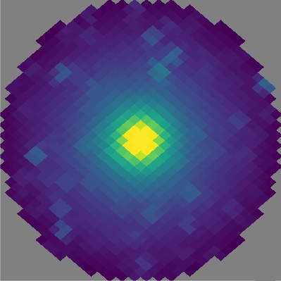
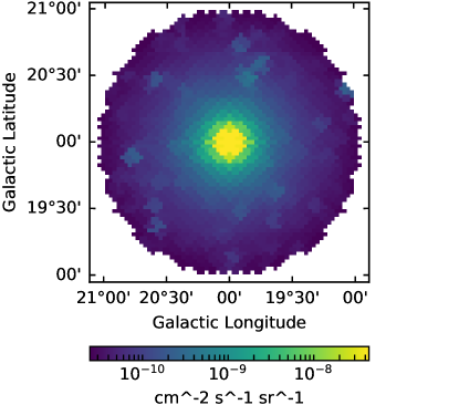
Figure 1: Illustration of the 2D map transformation using the makeFitsImage.py script. Top panel: 2D map output in the HEALPix format. Shown is the integrated $\gamma$-ray intensity of an example halo, drawn for the standard parameters in the -h5 module, using matplotlib and the healpy.cartview() function. Bottom panel: Transformed fits image, displayed with a simple Python script using matplotlib and astropy. Examples to generate above figures can be found in the CLUMPY online documentation.

5 New parameters and keywords

As in previous releases, CLUMPY comes with a large number of parameters required to perform any run: these include physics constants, dark matter halo properties, and simulation configurations. Some parameters require keywords that allow the user to select preset ingredients from the literature.

Table 1: CLUMPY parameters sorted by block (cosmology, dark matter, etc.). New parameters are highlighted in grey, deprecated ones in strikethrough. Note that this table is not comprehensive; a complete list of parameters is provided with the online documentation at http://lpsc.in2p3.fr/clumpy/.

Name	Definition
Cosmological parameters (updated from Planck results)
gCOSMO_HUBBLE	Present-day $(z=0)$ normalized Hubble expansion rate $h=H_{0}/(100\;{\rm km\;s}^{-1}\;{\rm Mpc}^{-1})$
gCOSMO_RHO0_C	Critical density of the universe, now calculated as $\varrho_{\rm c,0}=3H_{0}^{2}/(8\pi G)$
gCOSMO_OMEGA0_{M,B}	Present-day pressureless matter and baryon-only densities $\Omega_{\rm m,b}=\varrho_{\rm m,b}/\varrho_{\rm c}$
gCOSMO_OMEGA0​_LAMBDA	No longer input parameter, now calculated from $\sum_{i}\Omega_{i}=1$
gCOSMO_SIGMA8	Fluctuation amplitude, $\sigma_{8}$, at 8 h-1 Mpc
gCOSMO_N_S	Scalar spectral index $n_{\rm s}$ of primordial fluctuations
gCOSMO_T0	Present-day CMB photon temperature $T_{0}$ [K]
gCOSMO_TAU_REIO	Reionization optical depth $\tau_{\rm reio}$
gCOSMO_{DELTA0, FLAG_DELTA_REF}	Value $\Delta(z=0)$, and model to describe $\Delta(z)$, see Tab. 2 for possible keywords
Generic dark matter parameters (only new, renamed, or deprecated parameters are listed)
gDM_LOGCVIR_STDDEV gDM_LOGCDELTA_STDDEV	Width of log-normal $c_{\Delta}(M_{\Delta})$ distribution (value 0 corresponds to a Dirac distribution)
gDM_FLAG_CVIR_DIST	Redundant with gDM_LOGCDELTA_STDDEV
gDM_MMIN_SUBS gDM_SUBS_MMIN	Minimal mass of DM subhaloes [$M_{\odot}$]
gDM_MMAXFRAC_SUBS gDM_SUBS_MMAXFRAC	Maximal mass of subhalos in the host halo: $m_{\rm max}=~{}$gDM_SUBS_MMAXFRAC $\times\;M_{\rm host}$
gDM_IS_IDM	Use halo mass function cut-off for interacting DM according to [25]
gDM_KMAX	Modify scale $k_{\rm max}$ above which $P_{\rm lin}(k)$ is suppressed
Milky-Way DM halo and subhalo structural parameters (used in -g module): gGAL$\,\,\rightarrow\,\,$gMW for all parameters
gMW_TOT_{FLAG_PROFILE, RSCALE}	Description of the total DM density profile (see Tab. 2) and its scale radius, $r_{\rm s}$ [kpc]
gMW_TOT_SHAPE_PARAMS{​[0]​,​[1]​,​[2]​}​​_{0​,1​,2}	Shape parameters of the Milky Way total DM density profile
gMW_{RHOSOL, RSOL, RVIR​​RMAX}	Local DM density [GeV cm-3], distance GC–Sun [kpc], DM halo radius [kpc]
gMW_TRIAXIAL_{IS, AXES​​_{0​,1​,2}​​, ROTANGLES​​_{0​,1​,2}​​ }	Parameters related to triaxiality of the Milky Way DM host halo
gMW_CLUMPS​​SUBS​​_{FLAG_PROFILE, CVIRMIR​​CDELTAMDELTA​​}	Description of the subhalos’ density profile and $c_{\Delta}(m_{\Delta})$, see Tab. 2 for keywords
gMW_CLUMPS​​SUBS​​_SHAPE_PARAMS​​_{0​,1​,2}	Shape parameters of the Milky Way’s subhalos’ density profile (always spherical)
gMW_​​SUBS_​​DPDV_{FLAG_PROFILE, RSCALE​​_TO_RS_HOST​​}	Spatial subhalo distribution (see Tab. 2) in the Milky Way halo and ratio $a$ (see §4.3)
gMW_​​SUBS_​​DPDV_SHAPE_PARAMS​​_{0​,1​,2}	Shape parameters of the subhalos’ spatial distribution profile
gMW_​​SUBS_​​DPDM_SLOPE	Log-slope $\alpha$ of the subhalo mass function $\mathrm{d}\mathcal{P}/\mathrm{d}m\propto m^{-\alpha}$
gMW_SUBS_{M1, M2, N_INM1M2}	Number of Milky-Way subhaloes in $[m_{1},m_{2}]$
Structural parameters for dedicated halo types (mostly used in -h module): For TYPE = DSPH, GALAXY, CLUSTER, EXTRAGAL​​
gTYPE_TRIAXIAL_{IS, AXES{​[0]​,​[1]​,​[2]​}, ROTANGLES{​[0]​,​[1]​,​[2]​}	Deprecated: Triaxiality parameters of the host halo are set in gLIST_HALOES
gTYPE_CLUMPS​​SUBS​​_{FLAG_PROFILE, CVIRMIR​​CDELTAMDELTA​​}	Description of subhalos’ density profile in host and $c_{\Delta}(m_{\Delta})$, see keywords in Tab. 2
gTYPE_CLUMPS​​SUBS​​_SHAPE_PARAMS​​_{0​,1​,2}	Shape parameters of the host halo TYPE subhalos’ spherical density profile
gTYPE_​​SUBS_​​DPDV_{FLAG_PROFILE, RSCALE​​_TO_RS_HOST}​​​​	Spatial subhalo distribution (see Tab. 2) in host TYPE and ratio $a$ (see §4.3)
gTYPE_​​SUBS_​​DPDV_SHAPE_PARAMS​​_{0​,1​,2}	Shape parameters for the subhalos’ spatial distribution in the host
gTYPE_​​SUBS_​​DPDM_SLOPE	Log-slope $\alpha$ of the subhalo mass function $\mathrm{d}\mathcal{P}/\mathrm{d}m\propto m^{-\alpha}$
gTYPE_SUBS_MASSFRACTION	Mass fraction of the host halo TYPE contained in subhalos
Generic extragalactic physics parameters (used in -e module)
gEXTRAGAL_SUBS_DPDM_SLOPE_LIST	List of slopes of subhalo mass spectra $\mathrm{d}\mathcal{P}/\mathrm{d}M$ (to be used with the -e2 submodule)
gEXTRAGAL_FLAG_CDELTAMDELTA_LIST	List of $c_{\Delta}(m_{\Delta})$ models (to be used with the -e2 submodule)
gEXTRAGAL_FLAG_MASSFUNCTION	Halo mass function multiplicity function $f(\sigma,\,z)$, Eq. (4), see Tab. 2 for keywords
gEXTRAGAL_IDM_{MHALFMODE, ALPHA, BETA, GAMMA, DELTA}	Interacting DM halo mass function cut-off parameters, according to Eq. (11) of [25]
gEXTRAGAL_HMF_SMALLSCALE_DPDM_{SLOPE, MLIM}	Force halo mass function log-slope to be steeper than value below $M_{\rm lim}$, ($-1=$ off)
gEXTRAGAL_FLAG_ABSORPTIONPROFILE	EBL absorption profile $\tau(E_{\gamma},z)$, see Tab. 2 for possible keywords
Particle physics & spectral parameters: No changes w.r.t. last release, see Tab. (2) from [11] for the comprehensive list.
gPP_…
Statistical analysis (used in -s module): previously unnamed command-line parameters. Only a few are listed below.
gSTAT_{CL, CL_LIST}	Confidence level (or list of confidence levels) for statistical analysis
gSTAT_IS_LOGL_OR_CHI2	Choose between a likelihood or $\chi^{2}$-test based analysis
gSTAT_…	See online documentation for the comprehensive list
Draw halos from definition file
gLIST_{HALOES, HALOES_JEANS}	Text file defining halo properties for $J$-factor calculations or Jeans analysis
gLIST_HALONAME	Select a halo by name from above lists for analysis or drawing into 2D skymap
Global simulation parameters: gSIMU$\,\,\rightarrow\,\,$gSIM for all parameters of previous release. Extragalactic and a few other parameters are listed below.
gSIM_{NX, IS_XLOG, JFACTOR, REDSHIFT, … }	Set 1D grid, $J/D$, $z$, or other variables previously only accesible via the command line
gSIM_{PSI_OBS,THETA_OBS,THETA_ORTH_SIZE,THETA_SIZE}_DEG	Set FOV position and dimensions for 2D runs (previously only via the command line)
gSIM_EXTRAGAL_{ZMIN, ZMAX, NZ, IS_ZLOG}	Redshift range and grid for 2D analyses in $(M,z)$ plane
gSIM_EXTRAGAL_{MMIN, MMAX, NM, IS_MLOG}	Mass range and grid for 2D analyses in $(M,z)$ plane
gSIM_EXTRAGAL_{DELTAZ, NM}_PRECOMP	Resolution of redshift (lin) and mass (log) nodes for precalculated integration grid
gSIM_EXTRAGAL_FLAG_WINDOWFUNC	Spherical collapse model window function. See Tab. 2 for possible keywords
gSIM_EXTRAGAL_EBL_UNCERTAINTY	Systematic uncertainty on EBL extinction $\tau(z,E)$
gSIM_EXTRAGAL_FLAG_GROWTHFACTOR	Method to compute perturbation growth factor $g(z)$, Eq. (6), see Tab. 2 for keywords
gSIM_…	See online documentation for the comprehensive list

Parameters

In this release, we have made the following changes for the list of parameters, as shown in Tab. 1:

• For a better consistency and readability, we renamed some existing parameters (Milky way and generic halo structural parameters);

• In the course of homogenising the input parameter control as described in §6.3, many arguments previously solely specified via the command line are now given explicit parameter names.

• The most important changes are those associated with the many new parameters required to perform the extragalactic intensity calculation described in §2. We now have a more complete description of the cosmological parameters, extragalactic haloes structural parameters, and simulation parameters for the extragalactic calculation (lower part of the table).

Table 2: Enumerators and allowed keywords (with references) in the CLUMPY code. Curly brackets are used to group keywords having different endings.

Enumerator	Available keywords
New keywords in this release
gENUM_ABSORPTIONPROFILE​​​	kFRANCESCHINI{08, 17} [34, 35]​, kFINKE10 [38]​, kDOMINGUEZ11_{REF, LO, UP} [39]​,
	kGILMORE12_{FIDUCIAL, FIXED} [36]​, INOUE13_{REF, LO, UP} [37]
gENUM_DELTA_REF	kRHO_CRIT, kRHO_MEAN, kBRYANNORMAN98 [40]
gENUM_GROWTHFACTOR	kHEATH77 [42]​, kCARROLL92 [33]​, kPKZ_FROMFILE†
gENUM_MASSFUNCTION	kPRESSSCHECHTER74 [43]​, kSHETHTORMEN99 [44]​, kJENKINS01 [45]​,
	kTINKER{08, 08_N, 10} [46, 46, 47]​, kBOCQUET16_{HYDRO, DMONLY} [48]​,
	kRODRIGUEZPUEBLA16_PLANCK [49]
gENUM_WINDOWFUNC	kTOP_HAT, kGAUSS, kSHARP_K
Keywords already present in v1 and v2 (new keywords highlighed)
gENUM_ANISOTROPYPROFILE​​​	kCONSTANT, kBAES [50]​, kOSIPKOV [51, 52]
gENUM_LIGHTPROFILE	kEXP2D [53]​, kEXP3D [53]​, kKING2D [54]​, kPLUMMER2D [55]​, kSERSIC2D [56]​, kZHAO3D [57, 58]​​​​
gENUM_CDELTAMDELTA§	kB01_{VIR, ​VIR_RAD​} [59, 60]​, kENS01_VIR [61]​, kNETO07_200 [62]​,
	kDUFFY08F_{VIR,200,MEAN} [63]​, kETTORI10_200 [64]​, kPRADA12_200 [65]​, kGIOCOLI12_VIR [66]
	kPIERI11_{VIALACTEA,AQUARIUS} [67]​, kROCHA13_SIDM_VIR [68]​, kSANCHEZ14_200 [69]​,
	kCORREA15_PLANCK_200 [70]​, kLUDLOW16_200 [71]​, kMOLINE17_200 [72]
gENUM_PROFILE	kHOST, kZHAO [57, 58]​, kEINASTO [73]​, kEINASTO_N [74]​, kBURKERT [75]​, kISHIYAMA14 [76]​,
	kGAO_SUBkDPDV_GAO04‡ [77, 78]​,kDPDV_SPRINGEL08_FIT‡ [79]​,
	kEINASTOANTIBIASED_SUBkDPDV_SPRINGEL08_ANTIBIASED‡ [80, 81]
gENUM_TYPEHALOES	kDSPH, kGALAXY, kCLUSTER, kEXTRAGAL
gENUM_FINALSTATE	kGAMMA, kNEUTRINO
gENUM_NUFLAVOUR	kNUE, kNUMU, kNUTAU
gENUM_PP_SPECTRUMMODEL​​​​​​	kBERGSTROM98⋆ [82]​, kTASITSIOMI02⋆ [83]​, kBRINGMANN08⋆ [84], kCIRELLI11_{EW, NOEW} [12]

^† Look for files in data/pk_precomp, and if absent for user cosmology, generate $P(k,z)$ files with CLASS code [32].
^§ To be consistant with gENUM_DELTA_REF notation, we renamed gENUM_CVIRMVIR to gENUM_CDELTAMDELTA.
^‡ Applicable for the spatial distribution of subhaloes only.
^⋆ For $\gamma$-rays only (not enabled for $\nu$).

Keywords

The changes for the lists of keywords are reported in Tab. 2:

• The upper half of the table gathers the keywords associated to a model or parametrisation for the new extragalactic ingredients discussed in §3. They correspond to the absorption model (§3.2), the model to describe $\Delta(z)$ (Eq. 11), the growth factor (Eq. 6), the halo mass function parametrisation (Eq. 4), and the window function appearing in Eq. (5).

• The lower half of the table repeats the keywords to enumerators already presented in the previous version, with names having been changed for consistency (in particular for subhalo spatial distributions) and new keywords/parametrisations having been added. These changes are highlighted in grey.

6 Installation and code execution

We highlight in this section the changes made in this new release. Detailed instructions about the code structure, and how to install and execute it, are provided in the online documentation at http://lpsc.in2p3.fr/clumpy/.

6.1 Code installation, tests, and documentation

Several improvements have been made for the download, installation, and use of the CLUMPY C/C++ code.

• Public version control: the code is now under git version control, publicly accessible and currently at https://gitlab.com/clumpy/CLUMPY, from where the latest development versions can be directly retrieved.

• Compilation and dependencies: this new release of CLUMPY (C/C++) is compiled with cmake. It now only depends on the cfitsio and GSL libraries, with the ROOT library optional (some sub-modules, pop-up graphics, and outputs in ROOT format are available only when ROOT is installed). The dependency on HEALPix [85] is now ensured by a frozen version of the library (version 3.31) shipped with the code, which is internally built at compilation.

• General and code documentation: we have completely revisited the documentation, now based on sphinx. For developers, Doxygen pages are additionally generated and available from the documentation pages.

• Integration tests: we now provide an automated test suite, ./bin/clumpy_tests, to check the proper output of all modules after the installation.

6.2 Code structure and executables

As in the previous versions, declarations are stored in include/*.h (with the two new libraries cosmo.h and extragal.h), sources in src/*.cc, compiled libraries are saved in lib/, and executables in bin/. Tabulated tables on which CLUMPY relies (EBL, $P(k)$, PPPC4DMID spectra [86], reference test files…) are located in data/.

Beside the two executables for the Jeans analysis [11] (bin/clumpy_jeansChi2 and bin/clumpy_jeansMCMC) and the new module to test the successful installation (bin/clumpy_tests), the main executable is bin/clumpy, whose submodules are reproduced below for completeness:

• ./bin/clumpy -g[index]: galactic calculations,

• ./bin/clumpy -h[index]: isolated/list of haloes,

• ./bin/clumpy -s[index]: run on ‘statistical’ files,

• ./bin/clumpy -o[index]: skymap file manipulation,

• ./bin/clumpy -z: $\gamma$ and $\nu$ spectra,

• ./bin/clumpy -f: convert $J$-factor skymap to flux map,

and a new submodule provided in this release:

• ./bin/clumpy -e[index]: triggers the new extragalactic module and prints a list of available submodules (e0 to e6) if no index is put.

• ./bin/clumpy -e[index] -D: generates a file clumpy_params_e[index].txt containing all parameters and default values to execute the corresponding run. This is particularly useful for new users to familiarise themselves with the required ingredients necessary to each requested computation.

Running all executables without further options results in self-explanatory messages with instructions of how to run the various modules. Some explicit examples are given in §6.4.

6.3 Upgraded input parameter interface

To allow a better control of the manual execution of CLUMPY and a better interface to a pipelined execution of the code, CLUMPY input parameters can now be fully and flexibly controlled via the command line.

All parameters required for a specific run can be set in a parameter file, following the same format since the first version of the code or can alternatively be parsed via the command line; specifying a parameter value in the command line is always preferred over the parameter file (with a warning being drawn in the case of a double parameter setting). Also, the code now only requires the parameters needed for the specific executed run (and a warning is drawn for set, but unrelated parameters). In some cases, the requirement of a parameter depends on the value of another parameter, e.g., the number of shape parameters for a given DM density profile. These dependencies are now checked by the load_parameters() function at the beginning of each run execution, and default values are proposed after abort due to missing parameters. Also, default parameter files can be generated individually for each simulation mode with the -D flag.

This comprehensive expansion of the programming interface will finally also ease the construction of a wrapping Python module planned for a future release.

6.4 Run examples: extragalactic module

To illustrate the execution of the new extragalactic module and the refactored input interface described in the last paragraph, we present some examples below, for various indices for the submodules. For all modules, if CLUMPY is linked to ROOT, interactive pop-up graphics are directly displayed and/or the results are saved in ROOT format (results are always written to ASCII files). If not otherwise stated, below examples with default parameters provide results and pop-up graphics (like the shown Figs. 2 to 5) on the fly within a few seconds.

• ./bin/clumpy -e0 -i clumpy_params_e0.txt: computes the cosmological comoving, angular diameter, and luminosity distances, as well as the $\Omega$ and Hubble parameters at $z>0$, with all necessary input parameters read from clumpy_params_e0.txt.

• ./bin/clumpy -e1 -i clumpy_params_e1.txt: computes the halo mass function, Eq. (4). Two of the resulting ROOT pop-up graphics are displayed in Fig. 2. Note that a file is needed in the directory data/pk_precomp/ containing $P_{\rm lin}(k,z=0)$, where X denote the cosmological parameters specified in clumpy_params_e1.txt and Y is an arbitrary prefix. If no file is found, CLUMPY tries to run CLASS to generate it (with Y $=$ class). Any parameters in the parameter file can be overridden from the command line.

• ./bin/clumpy -e2 -i clumpy_params_e2.txt: Computes $c_{\Delta}(M_{\Delta},z)$, the luminosity $\mathcal{L}(M_{\Delta},z)$ (Eq. 7), and the boost, $\mathcal{L}_{\rm halo\,substructure}/\mathcal{L}_{\rm no\,substructure}$, over a user-defined mass range of extragalactic haloes. With this submodule, Fig. 1 from [11] is reproduced with a run time of about two minutes.

• ./bin/clumpy -e3 -i clumpy_params_e3.txt: computes the intensity multiplier, Eq. (3). The ROOT pop-up display with the result for the default parameters is shown in Fig. 3.

• ./bin/clumpy -e4 -i clumpy_params_e4.txt: computes the $\gamma$-ray EBL absorption exponent, $\tau(z,\,E_{\gamma})$, and $e^{-\tau(z,\,E_{\gamma})}$ from tabulated values (see §3.2).

• ./bin/clumpy -e5 -i clumpy_params_e5.txt: computes the differential contribution to the $\gamma$-ray or $\nu$ intensity from extragalactic DM, Eq. (1) or (2), from different redshift and mass shells, $\mathrm{d}I/\mathrm{d}z(z;\,\Delta M,\,E_{\gamma,\nu})$, and $\mathrm{d}I/\mathrm{d}M(M;\,\Delta z,\,E_{\gamma,\nu})$. This allows to get a better grasp of the contribution of different redshift and halo mass decades to the radiation intensity. For example, Fig. 4 shows that at $E_{\gamma}=10\,\mathrm{GeV}$, for the chosen branching channel and the displayed mass ranges, the ‘brightest’ redshift shell contributing to the $\gamma$-ray intensity lies between $0.2\lesssim z\lesssim 0.5$.

• ./bin/clumpy -e6 -i clumpy_params_e6.txt: fully integrates the $\gamma$-ray or $\nu$ intensity $I_{\rm ann}(E_{\gamma,\nu})$ from extragalactic DM, Eq. (1) or Eq. (2). The result for the default parameters, annihilation according to Eq. (1), is shown in Fig. 5.

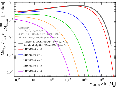
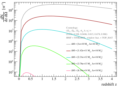
Figure 2: Pop-up graphics from the extragalactic -e1 module to study the halo mass function, Eq. (4). Top panel: Halo mass function from [46] (kTINKER08) at various redshifts $z$ between $z=0$ and $z=4$ and Planck 2015 [87] cosmological parameters. For comparison, the mass function at $z=0$ from the original publication [46] (and the cosmology chosen therein) is overplotted in grey. Bottom panel: Halo occupation (average number of haloes per redshift shell and solid angle) for different mass ranges, derived from the above halo mass function. In these plots, halo masses are defined with respect to the mean density, $\Delta(z)=200\times\Omega_{\rm m}(z)$, see Eq. (12).

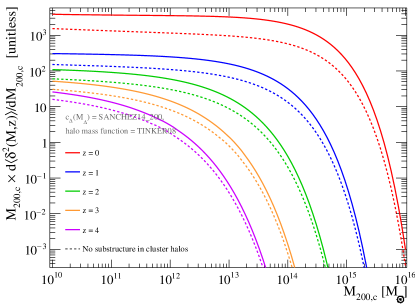
Figure 3: Pop-up graphic from the extragalactic -e3 module to study the intensity multiplier, Eq. (3), at various redshifts $z$ between $z=0$ and $z=4$. The solid lines show the intensity multiplier with the boost from halo substructure, while the dashed lines assume zero substructure boost. This result relies on the kTINKER08 [46] mass function and kSANCHEZ14_200 [69] $c_{\Delta}(M_{\Delta},z)$ parametrisation. The intensity multipliers are plotted over the halo masses with respect to the critical density, $\Delta(z)=200$, see Eq. (11).

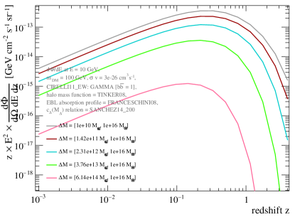
Figure 4: Pop-up graphic from the extragalactic -e5 module to study different redshift- and mass-range contributions to the $\gamma$-ray intensity $I=\mathrm{d}\Phi/\mathrm{d}E/\mathrm{d}\Omega$.

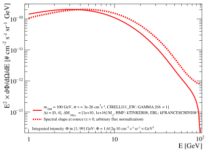
Figure 5: Pop-up graphic with the result of the extragalactic -e6 module and standard parameters to obtain the mean $\gamma$-ray intensity from extragalactic DM annihilation, Eq. (1) (solid line). The dashed line shows the spectral shape for the chosen annihilation channel ($\chi\chi\rightarrow b\bar{b}$) at $z=0$ and arbitrary normalisation. Note that in line with the user-specified multiplication of the differential intensity with $E^{n}$, the integrated intensity reported in the figure is calculated as $\Phi=\int E^{n}\,\mathrm{d}\Phi/(\mathrm{d}\Omega\,\mathrm{d}E)\,\mathrm{d}E$ (e.g., for $n=1$, $\Phi$ corresponds to the energy flux).

We have checked to the best of our ability that the CLUMPY calculations match the results previously found in the literature. For example, the red curve in the top panel of Fig. 2 does match the grey reference curve from [46] when using the appropriate cosmology. Similarly, in Fig. 6 of [19], we compared the extragalactic fluxes computed with this version of CLUMPY to several existing results and discuss the agreement or discrepancies in terms of parameter choices.

7 Conclusions

After ten years of development, the CLUMPY code now provides a comprehensive framework to compute indirect $\gamma$-ray and $\nu$ signals (from DM annihilation or decay) from the Galactic to the extragalactic scales.

In this new release, the code allows the flux and intensity calculation from haloes at any redshift, and to compute the average diffuse emission from all extragalactic DM. In doing so, the computation of various cosmological quantities had to be implemented, like halo mass functions with respect to any overdensity definition $\Delta$ and the optical depth to $\gamma$-rays due to pair production at the EBL. These intermediate quantities can be computed on their own, without seeking for $\gamma$-ray or $\nu$ signals from DM. By providing the corresponding submodules, we hope to widen the usage of the code at the interface between the astrophysics, astroparticle, and cosmology communities.

Moreover, the usage of the code has been simplified in several ways. Dependencies from third-party software have been made optional (ROOT) or hidden (HEALPix is shipped with the code), the compilation process has been improved, and an automated test suite is provided. Also, the input interface has been simplified, facilitating the isolated use of single modules and interfacing the code with other software. Finally, the documentation has also been fully rearranged and updated: it contains a comprehensive description of all features since the first release, step-by-step tutorials and usage examples, available output formats and transformations, as well as background information of numerical implementations and basic concepts. Also, we provide examples of how the code can be interfaced with Python.

With this third release, we hope to further improve the usage of CLUMPY as a comprehensive tool for indirect DM searches. Finally, let us stress that we welcome suggestions for new functionalities and incorporating new results from the community; any well-motivated request will be considered such that CLUMPY may keep evolving in-between major releases.

References

- [1] Lavalle, J. and Salati, P., Comptes Rendus Physique 13 (2012) 740.
- [2] Charles, E. et al., Phys. Rep.636 (2016) 1.
- [3] The ANTARES Collaboration, J. Cosmology Astropart. Phys.10 (2015) 068.
- [4] Aartsen, M. G., Ackermann, M., Adams, J., and etal, The European Physical Journal C 77 (2017) 627.
- [5] Charbonnier, A., Combet, C., and Maurin, D., Computer Physics Communications 183 (2012) 656.
- [6] Charbonnier, A. et al., MNRAS418 (2011) 1526.
- [7] Walker, M. G., Combet, C., Hinton, J. A., Maurin, D., and Wilkinson, M. I., ApJL 733 (2011) L46.
- [8] Combet, C. et al., Phys. Rev. D85 (2012) 063517.
- [9] Nezri, E. et al., MNRAS425 (2012) 477.
- [10] Maurin, D., Combet, C., Nezri, E., and Pointecouteau, E., A&A547 (2012) A16.
- [11] Bonnivard, V. et al., Computer Physics Communications 200 (2016) 336.
- [12] Cirelli, M. et al., J. Cosmology Astropart. Phys.3 (2011) 051.
- [13] Bonnivard, V. et al., MNRAS453 (2015) 849.
- [14] Bonnivard, V. et al., ApJ808 (2015) L36.
- [15] Bonnivard, V., Combet, C., Maurin, D., and Walker, M. G., MNRAS446 (2015) 3002.
- [16] Bonnivard, V., Maurin, D., and Walker, M. G., MNRAS462 (2016) 223.
- [17] Hütten, M., Combet, C., Maier, G., and Maurin, D., J. Cosmology Astropart. Phys.9 (2016) 047.
- [18] Esmaili, A. and Serpico, P. D., J. Cosmology Astropart. Phys.10 (2015) 014.
- [19] Hütten, M., Combet, C., and Maurin, D., J. Cosmology Astropart. Phys.2 (2018) 005.
- [20] Ullio, P., Bergström, L., Edsjö, J., and Lacey, C., Phys. Rev. D66 (2002) 123502.
- [21] Abdo, A. A. et al., J. Cosmology Astropart. Phys.4 (2010) 014.
- [22] Ng, K. C. Y. et al., Phys. Rev. D89 (2014) 083001.
- [23] The Fermi LAT Collaboration, J. Cosmology Astropart. Phys.9 (2015) 008.
- [24] Fornasa, M. and Sánchez-Conde, M. A., Phys. Rep.598 (2015) 1.
- [25] Moliné, Á., Schewtschenko, J. A., Palomares-Ruiz, S., Bœhm, C., and Baugh, C. M., J. Cosmology Astropart. Phys.8 (2016) 069.
- [26] Profumo, S. and Jeltema, T. E., J. Cosmology Astropart. Phys.7 (2009) 020.
- [27] Cirelli, M. and Panci, P., Nuclear Physics B 821 (2009) 399.
- [28] Belikov, A. V. and Hooper, D., Phys. Rev. D81 (2010) 043505.
- [29] Blanco, C., Harding, J. P., and Hooper, D., J. Cosmology Astropart. Phys.4 (2018) 060.
- [30] Hogg, D. W., ArXiv Astrophysics e-prints (1999).
- [31] Ando, S. and Komatsu, E., Phys. Rev. D87 (2013) 123539.
- [32] Lesgourgues, J., ArXiv e-prints (2011).
- [33] Carroll, S. M., Press, W. H., and Turner, E. L., ARA&A30 (1992) 499.
- [34] Franceschini, A., Rodighiero, G., and Vaccari, M., A&A487 (2008) 837.
- [35] Franceschini, A. and Rodighiero, G., A&A603 (2017) A34.
- [36] Gilmore, R. C., Somerville, R. S., Primack, J. R., and Domínguez, A., MNRAS422 (2012) 3189.
- [37] Inoue, Y. et al., ApJ768 (2013) 197.
- [38] Finke, J. D., Razzaque, S., and Dermer, C. D., ApJ712 (2010) 238.
- [39] Domínguez, A. et al., MNRAS410 (2011) 2556.
- [40] Bryan, G. L. and Norman, M. L., ApJ495 (1998) 80.
- [41] Knödlseder, J. et al., A&A593 (2016) A1.
- [42] Freedman, W. L. and Madore, B. F., ARA&A48 (2010) 673.
- [43] Press, W. H. and Schechter, P., ApJ187 (1974) 425.
- [44] Sheth, R. K. and Tormen, G., MNRAS308 (1999) 119.
- [45] Jenkins, A. et al., MNRAS321 (2001) 372.
- [46] Tinker, J. et al., ApJ688 (2008) 709.
- [47] Tinker, J. L. et al., ApJ724 (2010) 878.
- [48] Bocquet, S., Saro, A., Dolag, K., and Mohr, J. J., MNRAS456 (2016) 2361.
- [49] Rodríguez-Puebla, A. et al., MNRAS462 (2016) 893.
- [50] Baes, M. and van Hese, E., A&A 471 (2007) 419.
- [51] Osipkov, L. P., Pisma v Astronomicheskii Zhurnal 5 (1979) 77.
- [52] Merritt, D., AJ 90 (1985) 1027.
- [53] Evans, N. W., An, J., and Walker, M. G., MNRAS 393 (2009) L50.
- [54] King, I., AJ 67 (1962) 471.
- [55] Plummer, H. C., MNRAS 71 (1911) 460.
- [56] Sersic, J. L., Atlas de galaxias australes, Observatorio astronomico, Universidad de Cordoba, 1968.
- [57] Hernquist, L., ApJ 356 (1990) 359.
- [58] Zhao, H., MNRAS 278 (1996) 488.
- [59] Bullock, J. S. et al., MNRAS321 (2001) 559.
- [60] Kuhlen, M., Diemand, J., and Madau, P., ApJ686 (2008) 262.
- [61] Eke, V. R., Navarro, J. F., and Steinmetz, M., ApJ 554 (2001) 114.
- [62] Neto, A. F. et al., MNRAS 381 (2007) 1450.
- [63] Duffy, A. R., Schaye, J., Kay, S. T., and Dalla Vecchia, C., MNRAS 390 (2008) L64.
- [64] Ettori, S. et al., A&A 524 (2010) A68.
- [65] Prada, F., Klypin, A. A., Cuesta, A. J., Betancort-Rijo, J. E., and Primack, J., MNRAS 423 (2012) 3018.
- [66] Giocoli, C., Tormen, G., and Sheth, R. K., MNRAS422 (2012) 185.
- [67] Pieri, L., Lavalle, J., Bertone, G., and Branchini, E., Phys. Rev. D83 (2011) 023518.
- [68] Rocha, M. et al., MNRAS430 (2013) 81.
- [69] Sánchez-Conde, M. A. and Prada, F., MNRAS 442 (2014) 2271.
- [70] Correa, C. A., Wyithe, J. S. B., Schaye, J., and Duffy, A. R., MNRAS452 (2015) 1217.
- [71] Ludlow, A. D. et al., MNRAS460 (2016) 1214.
- [72] Moliné, Á., Sánchez-Conde, M. A., Palomares-Ruiz, S., and Prada, F., MNRAS466 (2017) 4974.
- [73] Navarro, J. F. et al., MNRAS349 (2004) 1039.
- [74] Merritt, D., Graham, A. W., Moore, B., Diemand, J., and Terzić, B., AJ 132 (2006) 2685.
- [75] Burkert, A., ApJL 447 (1995) L25.
- [76] Ishiyama, T., ApJ788 (2014) 27.
- [77] Gao, L., White, S. D. M., Jenkins, A., Stoehr, F., and Springel, V., MNRAS355 (2004) 819.
- [78] Madau, P., Diemand, J., and Kuhlen, M., ApJ679 (2008) 1260.
- [79] Springel, V. et al., MNRAS391 (2008) 1685.
- [80] Kuhlen, M., Diemand, J., and Madau, P., ApJ671 (2007) 1135.
- [81] Lange, J. U. and Chu, M.-C., MNRAS447 (2015) 939.
- [82] Bergström, L., Ullio, P., and Buckley, J. H., Astropart. Phys.9 (1998) 137.
- [83] Tasitsiomi, A. and Olinto, A. V., Phys. Rev. D 66 (2002) 083006.
- [84] Bringmann, T., Bergström, L., and Edsjö, J., J. High Energy Phys. 1 (2008) 49.
- [85] Górski, K. M. et al., ApJ622 (2005) 759.
- [86] Baratella, P. et al., J. Cosmology Astropart. Phys. 3 (2014) 53.
- [87] Planck Collaboration et al., A&A594 (2016) A13.