Efimov effect in a $D$-dimensional Born-Oppenheimer approach

Abstract

We study a three-body system, formed by two identical heavy bosons and a light particle, in the Born-Oppenheimer approximation for an arbitrary dimension $D$. We restrict $D$ to the interval $2\,<\,D\,<\,4$, and derive the heavy-heavy $D$-dimensional effective potential proportional to $1/R^{2}$ ($R$ is the relative distance between the heavy particles), which is responsible for the Efimov effect. We found that the Efimov states disappear once the critical strength of the heavy-heavy effective potential $1/R^{2}$ approaches the limit $-(D-2)^{2}/4$. We obtained the scaling function for the ¹³³Cs-¹³³Cs-⁶Li system as the limit cycle of the correlation between the energies of two consecutive Efimov states as a function of $D$ and the heavy-light binding energy $E^{D}_{2}$. In addition, we found that the energy of the $(N+1)^{\rm th}$ excited state reaches the two-body continuum independently of the dimension $D$ when $\sqrt{E^{D}_{2}/E_{3}^{(N)}}=0.89$, where $E_{3}^{(N)}$ is the $N^{\rm th}$ excited three-body binding energy.

• August 2018

1 Introduction

In the Landau and Lifshitz book on nonrelativistic quantum mechanics [1], one can read: “to reveal certain properties of quantum-mechanical motion it is useful to examine a case which, it is true, has no direct physical meaning: the motion of a particle in a field where the potential energy becomes infinite at some point (the origin) according to the law $U(r)\sim-\beta/r^{2}\,\,(\beta>0)$”. This book was first published in English language in 1958 and the transcribed sentence appears at the beginning of the subsection “fall of a particle to the centre”, in which the possible solutions of the Schrödinger equation for such a potential are studied. In particular, its was shown that the radial equation admits solutions of the form $r^{r_{0}+is}$, with $s$ being real for a range of values of the strength of the potential. In such a case, there are infinitely many bound states for the system with a spectrum unbounded from below. We recall that the “fall to the centre” phenomenon was found much earlier by Thomas in 1935 [2] for the triton in the limit of zero-range interaction between the nucleons. Later on, in 1970, Efimov found that a three-boson system presents an infinite number of three-body bound states for zero angular momentum [3] in the limit of infinite two-body scattering lengths —in this case an attractive long range potential proportional to $-1/\rho^{2}$, where $\rho$ is the hyper-radial coordinate, appears with a strength large enough to collapse the system analogously to the Landau example. The counterintuitive phenomenon discovered by Efimov appeared to be only a theoretical speculation added to the fact that the study was originally made in the nuclear physics context, where there is no possibility to have a two-body zero binding energy.

After almost thirty years since Efimov’s discovery, the experimental group from Innsbruck finally observed indirectly the formation of Efimov molecules in ultracold atomic traps [4] by using the Feshbach resonance phenomenon [5] to freely tune the two-body scattering lengths. The observation was made through the measurement of the three-body atomic loss peaks. These peaks appear as a consequence of the resonant three-body recombination process, where three atoms recombine forming a deep bound pair plus an atom with a recoil energy larger than the energy of the trap, resulting in the loss of three atoms each time this process happens. The positions where these peaks appear are given by the two-body scattering lengths, $a_{-}^{(N)}$, the subindex refers to negative scattering lengths, meaning that there are no shallow two-body bound states, and $N=0,1,2,\dots$ refers respectively to the ground, first, second, $\dots$ excited states. The ratio of consecutive $a_{-}^{(N)}$ follows the discrete Efimov scaling factor, $s$, and is given by $a_{-}^{(N+1)}/a_{-}^{(N)}={\rm exp}(\pi/s)$ [6, 7]. Thus, the observation of the position of the recombination peaks allows an indirect verification of the Efimov phenomenon. Nowadays, very advanced techniques allow the direct measurement of the binding energy of the three- and two-body molecules in atomic clouds [8, 9].

Fonseca and collaborators showed in a seminal paper [10] that the similarity between the Landau’s “fall to the centre” and the general picture given by Efimov could be extended to strongly mass asymmetric systems, where the Born-Oppenheimer approximation applies. The authors of Ref. [10] have shown that the exchange of the light particle between the heavy ones generates an effective potential proportional to $-1/R^{2}$, where $R$ is the separation distance between the heavy particles, which causes the accumulation of the three-body levels close to the continuum. Not only the form of the potential matters to have infinitely many three-body bound states but also the strength, which is directly related to the Efimov discrete scaling factor. In three-spatial dimensions, the form of the potential is presently well-known to be $-(s^{2}+1/4)/R^{2}$, and Efimov states with the characteristic log-periodic behavior will be present when $s^{2}>0$.

Nowadays, there is an increasing interest in studying weakly bound few-body systems in spatial dimension different than three [11]. Experimentally, dimensional transition can be obtained in ultracold atomic clouds in a confining potential squeezed asymmetrically in one or two directions. Consequentely, the atomic clouds can be compressed, or expanded, in such a way the effective-spatial dimension felt by the system is continuously changed [12].

Nielsen and collaborators [13] showed that for three identical bosons the Efimov effect exists in the interval $2.3\,<\,D\,<\,3.8$, recently this result has been proven using a different approach [14]. More recently, we have extended this result to a heteroatomic $AAB$ system [15] based on the Danilov’s solution [16] of the Skornyakov and Ter-Martirosyan three-boson integral equation [17] in the ultraviolet region. In Ref. [15] we have determined the dimensional boundaries as a function of the atomic mass ratio, $\mathpzc{A}=m_{B}/m_{A}$, for which the Efimov effect exists, and the corresponding Efimov discrete scaling factor was obtained as a function of $\mathpzc{A}$ and $D$.

In the present work we study, in $D$ dimensions, a three-body $AAB$ system formed by two-identical heavy atoms $A$ and a different one $B$ in the Born-Oppenheimer approximation. This work extends our previous study in Ref. [15] in several directions. First, we depart from the ideal case without scales studied in that reference. We generalize the work by Fonseca, Redish and Shanley [10] to arbitrary $D$ spatial dimensions and mass ratios $\mathpzc{A}=m_{B}/m_{A}$, and calculate the effective heavy-heavy potential responsible for the appearance of the Efimov effect. We also obtain the $D$ and $\mathpzc{A}$ dependence of the critical strength for the existence of Efimov states, which for $D=3$ was determined by Landau and Lifshitz [1] to be $-1/4$. For completeness, we have also show that the new results agree in the appropriate limits with those in Ref. [15]. In addition, we obtain the full three-body spectrum. The spectrum reveals a new and very counterintuitive result, in that the ratio of the two-body binding energy $E^{D}_{2}$ to the $N-$th excited three-body energy $E_{3}^{(N)}$ for which the Efimov effect disappears is independent of $D$.

The article is organized as follows. In Section II we describe our formalism: the effective potential, coming from the light-atom equation, is extracted in momentum space for a zero-range interaction between the light-heavy atoms. The small distance regime of the effective potential gives the critical strengths for which the Efimov effect exists. In Section III we present the Efimov discrete scaling factor for a general value of $D$ and calculate the three-body energy spectrum using a $D$-dimensional Schrödinger equation. In section IV we summarize and conclude.

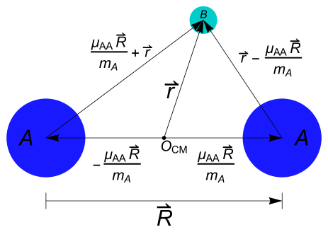
Figure 1: Three-body system formed by two identical heavy bosons with mass $m_{A}$ and an particle with mass $m_{B}$. We are considering the Born-Oppenheimer validity range where $m_{B}/m_{A}\ll 1$.

2 The Born-Oppenheimer approximation

We consider a system formed by two-heavy bosons and a light particle, pictorially represented in Fig. 1. We employ the Born-Oppenheimer approximation; which allows us to separate the full three-body Schrödinger equation into two equations, one for the heavy-light subsystem

$$\left[-\frac{\hbar^{2}}{2\mu_{B,AA}}\nabla^{2}_{r}+V_{AB}(\vec{r}-\frac{\mu_{AA}}{m_{A}}\vec{R})+V_{AB}(\vec{r}+\frac{\mu_{AA}}{m_{A}}\vec{R})\right]\psi_{R}(\vec{r})=\epsilon(R)\psi_{R}(\vec{r}),$$ (1)

and another for the two heavy particles:

$$\left[-\frac{\hbar^{2}}{2\mu_{AA}}\nabla^{2}_{R}+V_{AA}(\vec{R})+\epsilon(R)\right]\phi(\vec{R})=E_{3}\phi(\vec{R}),$$ (2)

where the reduced masses are given by $\mu_{AA}=m_{A}/2$ and $\mu_{B,AA}=2m_{A}m_{B}/\left(2m_{A}+m_{B}\right)$, and $V_{AB}$ and $V_{AA}$ denote in an obvious notation the $AB$ and $AA$ two-body interactions, respectively. As usual with the Born-Oppeheimer approximation, $R$ enters as parameter in Eq. (1) and can be used as a labelling index, and the eigenvalue $\epsilon(R)$ of the heavy-light equation enters as an effective potential in Eq. (2) for the heavy-heavy system. We employ a contact interaction with strength $\lambda$ for the heavy-light potential $V_{AB}$ so that one can write Eq. (1) in momentum space as

$$\frac{q^{2}}{2\mu_{B,AA}}\tilde{\psi}_{R}(\vec{q})+\lambda\left[e^{i\vec{q}\cdot\vec{R}/2}\,A_{R}^{(+)}+e^{-i\vec{q}\cdot\vec{R}/2}\,A_{R}^{(-)}\right]=\epsilon(R)\tilde{\psi}_{R}(\vec{q}),$$ (3)

where

$$A_{R}^{(\pm)}=\int\frac{d^{D}q}{(2\pi)^{D}}\,e^{\mp i\vec{q}\cdot\vec{R}/2}\,\tilde{\psi}_{R}(\vec{q}),$$ (4)

with $\tilde{\psi}_{R}(\vec{q})$ being the Fourier transform of $\psi_{R}(\vec{r})$, defined as

$$\psi_{R}(\vec{r})=\int\frac{d^{D}q}{(2\pi)^{D/2}}\,e^{i\vec{q}\cdot\vec{r}}\,\tilde{\psi}_{R}(\vec{q}).$$ (5)

The eigenvalue $\epsilon(R)$ can be determined as follows [18]. Initially, one rewrites Eq. (3) as

$$\tilde{\psi}_{R}(\vec{q})=\lambda\,\frac{e^{i\vec{q}\cdot\vec{R}/2}A_{R}^{(+)}+e^{-i\vec{q}\cdot\vec{R}/2}\,A_{R}^{(-)}}{\epsilon(R)-\frac{q^{2}}{2\mu_{B,AA}}}.$$ (6)

Next, one eliminates $\tilde{\psi}_{R}(\vec{q})$ in favor of $A_{R}^{(\pm)}$ using Eq. (4):

$$A_{R}^{(\pm)}=\lambda\int\frac{d^{D}q}{(2\pi)^{D}}\;\frac{A_{R}^{(\pm)}+e^{\mp i\vec{q}\cdot\vec{R}}\,A_{R}^{(\mp)}}{\epsilon(R)-\frac{q^{2}}{2\mu_{B,AA}}}.$$ (7)

Then, it is easily shown that for nontrivial solutions, $A_{R}^{(\pm)}\neq 0$, the eigenvalue is given by the transcendental equation:

$$\frac{1}{\lambda}=\int\frac{d^{D}q}{(2\pi)^{D}}\,\frac{\cos(\vec{q}\cdot\vec{R})+1}{\epsilon(R)-\frac{q^{2}}{2\mu_{B,AA}}}.$$ (8)

The integral is divergent but the divergence can be dealt with by eliminating the strength $\lambda$ in favor of the two-body binding energy. That is, assuming that the two-body subsystem contains a bound state with energy $E_{AB}\equiv-|E^{D}_{2}|$

$$\frac{1}{\lambda}=-\int\frac{d^{D}q}{(2\pi)^{D}}\,\frac{1}{|E^{D}_{2}|+\frac{q^{2}}{2\mu_{B,AA}}},$$ (9)

and using this to replace $1/\lambda$ in Eq. (8) one obtains

$$\int\frac{d^{D}q}{(2\pi)^{D}}\left[\frac{\cos(\vec{q}\cdot\vec{R})+1}{\epsilon(R)-\frac{q^{2}}{2\mu_{B,AA}}}+\frac{1}{|E^{D}_{2}|+\frac{q^{2}}{2\mu_{B,AA}}}\right]=0.$$ (10)

The integral in Eq. (10) can be solved analytically; the result is

$$2^{D/2}{\bar{R}}^{1-D/2}|\bar{\epsilon}({\bar{R}})|^{(D-2)/4}K(D/2-1,{\bar{R}}|\bar{\epsilon}({\bar{R}})|^{1/2})$$

$$-\pi\csc\left(D\pi/2\right)\frac{1}{\Gamma(D/2)}\,\left(1-|\bar{\epsilon}({\bar{R}})|^{D/2-1}\right)=0 ,\;\;\;\;\;$$ (11)

where $|\bar{\epsilon}(R)|=|\epsilon(R)|/|E^{D}_{2}|$ and ${\bar{R}}=R/a$ with $a=\sqrt{\hbar^{2}/{2\mu_{B,AA}|E^{D}_{2}|}}$. $K(z)$ and $\Gamma(z)$ are, respectively, the modified Bessel function of the second kind and the gamma function.

The effective potential $\bar{\epsilon}(R)$ is obtained from the transcendental equation in Eq. (10) that can be solved for a given mass ratio $\mathpzc{A}=m_{B}/m_{A}$ and dimension $D$. The effective potential assumes quite simple forms in the limits of large and small ${\bar{R}}$. In the following, we investigate both limits and compare them with the well known results for $D=3$ and $D=2$.

Large distances regime, ${\bar{R}}\gg 1$. For large ${\bar{R}}$ the light atom bounds to only one of the heavy atoms in such a way the three body problem is roughly reduced to a two body problem with $|E_{3}|\rightarrow|E^{D}_{2}|$. The effective potential can then be written as $\lim_{{\bar{R}}\rightarrow\infty}|\epsilon({\bar{R}})|=|E^{D}_{2}|+V({\bar{R}})$, with $V({\bar{R}})\rightarrow 0$ for ${\bar{R}}\rightarrow\infty$. Replacing this asymptotic result in Eq. (11) we have that the effective potential can be written as

$$|\bar{\epsilon}_{{}_{{\bar{R}}\rightarrow\infty}}({\bar{R}})|=1+\frac{K\left(D/2-1,{\bar{R}}\right)}{d(D,\bar{R})},$$ (12)

where

$$d(D,\bar{R}) = \frac{{\bar{R}}}{2}K(D/2,{\bar{R}})+(1-D/2)$$ (13)

$$\times\Biggl{[}\frac{\pi\csc(D\pi/2)}{2^{D/2}{\bar{R}}^{(1-D/2)}\Gamma(D/2)}$$

$$+\,K(D/2-1,{\bar{R}})\Biggr{]}.$$

For $D=3$, one obtains well-known result of Ref. [10]:

$$|\bar{\epsilon}_{{}_{{\bar{R}}\rightarrow\infty}}({\bar{R}})|^{D=3}=1+\frac{2}{{\bar{R}}}e^{-{\bar{R}}},$$ (14)

and for $D=2$, the result of Ref. [18]:

$$|\bar{\epsilon}_{{}_{{\bar{R}}\rightarrow\infty}}({\bar{R}})|^{D=2}=1+\frac{2K(0,{\bar{R}})}{1+{\bar{R}}K(1,{\bar{R}})}.$$ (15)

Small distances regime, ${\bar{R}}\rightarrow 0$. This regime is directly related to the appearance of the Efimov effect. For $D=2$ the potential presents a Coulombic behaviour reproducing exactly a previous result obtained in Ref. [19], namely:

$$|\bar{\epsilon}_{{}_{{\bar{R}}\rightarrow 0}}({\bar{R}})|^{D=2}=\frac{2}{{\bar{R}}}e^{-\gamma},$$ (16)

where $\gamma=0.57721\cdots$ is the Euler-Mascheroni number. For values of $D$ in the interval $2<D<4$, it is convenient rewrite Eq. (11) as

$$\frac{|\bar{\epsilon}(\bar{R})|^{D/4-1/2}}{1-|\bar{\epsilon}(\bar{R})|^{D/2-1}}=\frac{\pi\csc(\pi D/2)\bar{R}^{D/2-1}}{2^{D/2}\Gamma(D/2)K(D/2-1,\bar{R}{|\bar{\epsilon}(\bar{R})|^{1/2}})}.$$ (17)

As the effective potential diverges at short distances, one can isolate $|\bar{\epsilon}(\bar{R})|$ in Eq. (17) and write

$$|\bar{\epsilon}_{R\rightarrow 0}(\bar{R})|=\frac{g(D)}{\bar{R}^{2}},$$ (18)

where $g(D)$ is the solution of the transcendental equation

$$g(D)=\left[-\frac{\pi\csc(D\pi/2)}{2^{D/2}\Gamma({D}/{2})K(D/2-1,\sqrt{g(D)})}\right]^{\frac{4}{2-D}}.$$ (19)

For $D=3$, one obtains

$$g(3)=0.3216,$$ (20)

which reproduces the $D=3$ results [10, 7]. The effective strength $g(D)$ plays here a central role in the occurance of the Efimov effect for $D>2$. This will be discussed in the next section.

3 Efimov effect for $D$ Spatial Dimensions

The $D$-spherical Schrödinger equation [20] for zero total angular momentum is given by

$$\left[-\frac{\hbar^{2}}{2\mu_{AA}}\nabla^{2}_{R}+\epsilon(R)\right]\phi(\textbf{R})=E\phi(\textbf{R}),$$ (21)

where the radial part of the Laplacian reads

$$\nabla^{2}_{R}=\frac{d^{2}}{dR^{2}}+\frac{D-1}{R}\frac{d}{dR}.$$ (22)

For two identical heavy particles and considering an infinitely high excited three-body state with energy $E_{3}\approx 0$ we can write

$$\left[\frac{d^{2}}{dR^{2}}+\frac{D-1}{R}\frac{d}{dR}-\frac{2\mu_{AA}}{\hbar^{2}}\epsilon(R)\right]\phi(R)=0.$$ (23)

The effective potential in the regions where the Efimov effect appears (small distances) is given by Eq. (18), $-{\cal G}/R^{2}$, where ${\cal G}$ depends on the mass ratio and dimension. Replacing the asymptotic effective potential and using the ansatz $\phi(R)=R^{\delta}$ we can calculate the Efimov discrete scaling factor $s$ for a general $D$ $(2<D<4)$.

$$\delta=\frac{1}{2}\pm i\sqrt{\frac{\mathpzc{A}+2}{4\mathpzc{A}}g(D)-(D/2-1)^{2}}=\frac{1}{2}\pm is.$$ (24)

In order to have the Efimov effect, $\phi(R)$ should oscillate, thus $s$ should be real. As an example, Figure 2 shows for a ¹³³Cs-¹³³Cs-⁶Li system, $\mathpzc{A}=6/133$, the region where the Efimov effect is allowed. The difference of the $D$ limits of the BO approximation with the exact result [15] is less than 2%. Note that the effect of a finite $E^{D}_{2}$ is washed out here as the critical strength is obtained in the limit of ${\bar{R}}\rightarrow 0$.

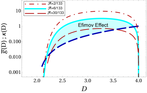
Figure 2: The shadowed area shows the region where the Efimov effect is allowed according to the effective strength given by Eq. (18). The blue dashed line is the critical strength given by $\kappa(D)=(D-2)^{2}/4$ Eq. (24), and the effective strength ${\bar{g}}(D)=(\mathpzc{A}+2)g(D)/4\mathpzc{A}$ is presented for three different mass ratios. The dimensional limit is $2.21<D<3.90$ for $\mathpzc{A}=6/133$.

Our previous results generalizing the Efimov discrete scaling factor were obtained in the ideal unitary limit [15], where all the energies are washed out of the problem. As energies are always finite in experiments, in this section we generalize the Schrödinger equation to $D$ spatial dimensions to obtain the three-body energy spectrum:

$$\left[-\frac{d^{2}}{dR^{2}}-\frac{D-1}{R}\frac{d}{dR}+\frac{m_{A}}{\hbar^{2}}\epsilon(R)+\frac{l(l+D-2)}{R^{2}}\right]\phi(R)=\frac{m_{A}}{\hbar^{2}}E_{3}\,\phi(R).$$ (25)

Replacing $\phi(R)=\chi(R)/R^{(D-1)/2}$, this equation becomes

$$\left[-\frac{d^{2}}{dR^{2}}+\frac{f(D,l)}{R^{2}}+\frac{m_{A}\epsilon(R)}{\hbar^{2}}\right]\chi(R)=\frac{m_{A}E_{3}}{\hbar^{2}}\chi(R),$$ (26)

where $f(D,l)=[D^{2}-4D+3+4l(l+D-2)]/4$. Note that $f(D,l)$ reduces to the well-known results $f(2,l)=(-1+4l^{2})/4$ and $f(3,l)=l(l+1)$. Rescaling $R$ and $\epsilon(R)$ as in the previous section, Eq. (26) can be rewritten as

$$\left[-\frac{d^{2}}{d\bar{R}^{2}}+\frac{f(D,l)}{\bar{R}^{2}}+\frac{m_{A}}{2\mu_{B,AA}}\bar{\epsilon}(\bar{R})\right]\chi(\bar{R})=\frac{m_{A}}{2\mu_{B,AA}}\frac{E_{3}}{|E^{D}_{2}|}\chi(\bar{R}).$$ (27)

The potential diverges for ${\bar{R}}\rightarrow 0$ and needs to be regularized. We choose a regularization function of the form $1-e^{-(R/R_{0})^{3}}$, where the parameter $R_{0}$ is related to the van de Waals length that cuts off the very short distance region related to the chemistry of the heavy atoms. Higher powers of the regularization function can be compensated with a slight change of $R_{0}$ in order to preserve the present results. The regularized Schrödinger equation in $D$ dimensions is given by

$$\left[-\frac{d^{2}}{d\bar{R}^{2}}+\frac{f(D,l)}{\bar{R}^{2}}+\frac{m_{A}}{2\mu_{B,AA}}\left(1-e^{-(\bar{R}/\bar{R}_{0})^{3}}\right)\bar{\epsilon}(\bar{R})\right]\chi(\bar{R})=\frac{m_{A}}{2\mu_{B,AA}}\frac{E_{3}}{|E^{D}_{2}|}\chi(\bar{R}),$$ (28)

with $\bar{R}_{0}=R_{0}/a$, where $a$ was defined below Eq. (11).

The three-body energy calculated from Eq. (28) can be represented in terms of a universal scaling function for two consecutive trimer energies $E_{3}^{(N)}$ and $E_{3}^{(N+1)}$, where higher indexes indicate higher excited states (see e.g. [21]), as

$$\lim_{N\rightarrow\infty}\sqrt{\frac{E_{3}^{(N+1)}-E^{D}_{2}}{E_{3}^{(N)}}}={\cal F}\left(\sqrt{\frac{E^{D}_{2}}{E_{3}^{(N)}}},\,D,\,\mathpzc{A}\right).$$ (29)

It is important to note that the limit in Eq. (29) is reached very fast and defines the universal scaling function ${\cal F}$, obtained numerically, as showed in Fig. 3.

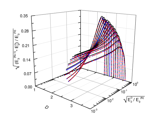
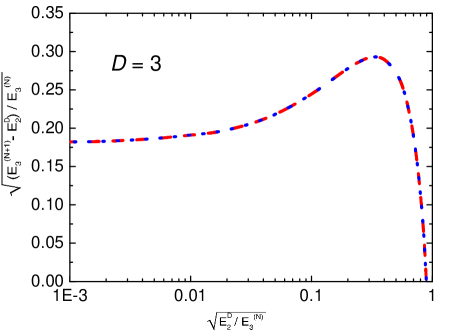
Figure 3: Upper frame: three-body energies for the ¹³³Cs-¹³³Cs-⁶Li system, $\mathpzc{A}=6/133$, for different dimensions. The energies are obtained from the numerical solution of Eq. (28). The solid black, dashed red and dotted blues lines are, respectively, results for $N=0,\,1$ and 2. Lower frame: curve for $D=3$.

The upper frame of Fig. 3 was constructed using $N=0,\,1$ and 2, and the corresponding results are represented by the solid (black), dashed (red) and dotted (blue) lines, respectively. The coincidence between dashed and dotted lines shows that the limit cycle is already obtained for $N=1$. The curve for $D=3$ is showed in the lower frame of Fig. 3 where the constant three-body energy ratio becomes evident once the magnitude of $E^{D}_{2}/E_{3}^{(N)}$ decreases. The Efimov discrete scaling factor, $s$, can then be extracted using Eqs. (18) and (24) or checking the three-body energy ratios for small $E^{D}_{2}$ - both methods give exactly the same result, which differs from the exact calculation by less than 2% [15] for the boundaries of existence of the Efimov effect.

It is important to note that the universal point where an excited three-body state disappears at the two-body energy cut does not depend on the dimension of the system, it depends only on the mass ratio. For $\mathpzc{A}=6/133$ the critical point is given by $\sqrt{E^{D}_{2}/E_{3}^{(N)}}=0.89$. Possible effects coming from a finite $E^{D}_{2}$ at the threshold for the disappearance of an excited state, observed in Ref. [6], are not increased by the dimensional change as the critical points do not depend on $D$.

The connection of the results presented in this article with the experiment can be made clear when we compare the energy spectrum of the three-body system found in this work with the three-body spectrum of a full 3D calculation in the presence of a external trap [22]. In Fig. 4 we present in the upper frame the three-body energy spectrum for a ¹³³Cs-¹³³Cs-⁶Li system [23] for fractional dimension when the two-body energy depends on the dimension, in the lower frame the three-body energy spectrum is presented when the two-body energy depends on the squeezed parameter $b_{\omega}$ for the ¹³³Cs-¹³³Cs-⁶Li system. The results presents similar qualitative results mostly in the limit of two and three dimensions. The connection for fractional dimensions [24] is not clear once the relation of the dimension with the squeezed parameter of the trap is not clear and is not the aim of this work to prove such relation once this would demand an elaborate calculation for three particles in external fields implying complications as four-body problem [25]. On the other hand, when a three-body system in the presence of an external trap approaches two dimensions, the infinite bound states present in fractional dimensions need to fit into the four possible bound states in two dimensions, causing an avoided crossing effect that becomes quite sharp in Ref. [22] when the energy of three-body is calculated for fixed values of the two-body energy. However, we note that the more realistic case when the energy of two-body depends on $b_{\omega}$ and $D$ this effect is smoothed when studying the energy of the trimer with respect of the two-body energy.

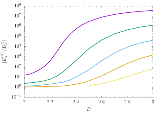
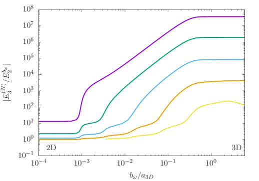
Figure 4: Three-body energy spectrum normalized to the two-body energies in $D$ dimensions for $\mathpzc{A}=6/133$. Upper panel: spectrum calculated with the Schrödinger equation in Eq. (28). Lower panel: spectrum calculated with a full Faddeev calculation [22] in a cubic box, where $b_{\omega}$ is the equivalent squeezing parameter of a harmonic trap—see text for explanations.

4 Conclusions

In this article we used the Born-Oppenheimer approximation to study a heavy-heavy-light system. We derived the effective heavy-heavy potential for $D$ dimensions that allows the appearance of the Efimov effect. The effective potential gives also the dimensional interval where the Efimov effect is possible. Our results generalize the pioneering work of Fonseca and collaborators [10] that deduced long ago the form of the effective long-range potential close to the unitary limit in three-dimensions. The present effective potential reproduces the well-known results for two and three dimensions. We applied the present analysis to the ¹³³Cs-¹³³Cs-⁶Li system and computed the scaling function obtained as a limit cycle of the correlation between the energies of two successive Efimov states with dependence on the heavy-light binding energy and dimension. We found that for $\sqrt{E^{D}_{2}/E_{3}^{(N)}}=0.89$ the $(N+1)$th excited state reach the two-body continuum, curiously, independent of the dimension. For D=3, Refs. [26, 27] have studied the Efimov physics of the four-body mass-asymmetric systems. However, it still remains as a challenge the study of dimensionality reduction for bound mass-asymmetric systems beyond three bodies.

References

References

- [1] L D Landau and E M Lifshitz 1977 Quantum Mechanics (Pergamon Press, London).
- [2] L H Thomas 1935 The Interaction Between a Neutron and a Proton and the Structure of Phys. Rev. 47 903
- [3] V Efimov 1970 Energy levels arising from resonant two-body forces in a three-body system Phys. Lett. B 33 563
- [4] T Kraemer, M Mark, P Waldburger, J G Danzl, C Chin, B Engeser, A D Lange, K Pilch, A Jaakkola, H-C Nägerl and R Grimm 2006 Evidence for Efimov quantum states in an ultracold gas of caesium atoms Nature 440 315
- [5] C Chin, R Grimm, P Julienne and E Tiesinga 2010 Feshbach resonances in ultracold gases Rev. Mod. Phys. 82 1225
- [6] J Ulmanis, S Häfner, R Pires, E D Kuhnle, Yujun Wang, Chris H Greene and M Weidemüller 2016 Heteronuclear Efimov Scenario with Positive Intraspecies Scattering Length Phys. Rev. Lett. 117 153201
- [7] S Häfner, J Ulmanis, E D Kuhnle, Y Wang, C H Greene and M Weidemüller 2017 Role of the intraspecies scattering length in the Efimov scenario with large mass difference Phys. Rev. A 95 062708
- [8] M Kunitsli et al 2015 Observation of the Efimov state of the helium trimer Science 348 551
- [9] S Zeller et al 2016 Imaging the quantum halo state using a free electron laser Proc. Natl. Acad. Sci. 113 14651
- [10] A C Fonseca, E F Redish and P E Shanley 1979 Efimov Effect in an Analytically Solvable Model Nucl. Phys. A320 273
- [11] F S Moller, D V Fedoror A S Jensen and N T Zinner 2018 Correlated gaussian approach to anisotropic resonantly interacting few-body systems arXiv:1805.12488 [cond-mat.quant-gas]
- [12] C J Pethick and H Smith 2008 Bose-Einstein Condensation in Dilute Gases (Cambridge).
- [13] E Nielsen, D V Fedorov, A S Jensen and E Garrido 2001 The three-body problem with short-range interactions Phys. Rep. 347 373
- [14] A Mohapatra and E Braaten 2018 Conformality Lost in Efimov Physics Phys. Rev. A 98 013633
- [15] D S Rosa, T Frederico, G Krein and M T Yamashita 2018 Efimov effect in spatial dimensions in systems Phys. Rev. A 97 050701(R)
- [16] G S Danilov 1961 On the Three-Body Problem with Short-Range Forces Sov. Phys. JETP 13 349
- [17] G V Skornyakov and K A Ter-Martirosyan 1957 Sov. Phys. JETP 31 775 1956 Sov. Phys. JETP 4 648
- [18] F F Bellotti, T Frederico, M T Yamashita, D V Fedoror A S Jensen and N T Zinner 2013 Mass-imbalanced three-body systems in two dimensions J. Phys. B 46 055301
- [19] D S Rosa, F F Bellotti, A S Jensen, G Krein and M T Yamashita 2016 Bound states of a light atom and two heavy dipoles in two dimensions Phys. Rev. A 94 062707
- [20] J Martins, H V Ribeiro, L R Evangelista, L R da Silva and E K Lenzi 2012 Fractional Schrödinger equation with noninteger dimensions App. Math. Comput. 219 2313
- [21] T Frederico, L Tomio, A Delfino, M R Hadizadeh and M T Yamashita 2011 Scales and universality in few-body systems Few-Body Syst. 51 87
- [22] J H Sandoval, F F Bellotti, M T Yamashita, T Frederico, D V Fedorov A S Jensen and N T Zinner 2018 Squeezing the Efimov effect J. Phys. B: At. Mol. Opt. Phys. 51 065004
- [23] S K Tung, K Jiménez-Garcıí a, J Johansen, C V Parker and C Chin 2014 Geometric Scaling of Efimov States in a 6Li-133Cs Mixture Phys. Rev. Lett. 113 240402
- [24] J Levinsen, P Massignan and M Parish 2014 Efimov Trimers under Strong Confinement Phys. Rev. X 4 031020
- [25] E R Christensen, A S Jensen and E Garrido 2018 Efimov states of three unequal bosons in non-integer dimensions arXiv:1805.12488 [cond-mat.quant-gas]
- [26] Y Wang, W B Laing, J von Stecher and B D Esry 2012 Efimov Physics in Heteronuclear Four-Body Systems Phys. Rev. Lett. 108 073201
- [27] D Blume and Y Yan 2014 Efimov Physics in Heteronuclear Four-Body Systems Phys. Rev. Lett. 113 213201